a computational tool for the reduction of …matrhc/clewleyrrotsteinhgkopelln... · a computational...

A COMPUTATIONAL TOOL FOR THE REDUCTION OF NONLINEAR ODE

SYSTEMS POSSESSING MULTIPLE SCALES

ROBERT CLEWLEY†‡ , HORACIO G. ROTSTEIN† , AND NANCY KOPELL†

Abstract. Near an orbit of interest in a dynamical system, it is typical to ask which variables dominateits structure at what times. What are its principal local degrees of freedom? What local bifurcation structureis most appropriate? We introduce a combined numerical and analytical technique that aids the identification ofstructure in a class of systems of nonlinear ordinary differential equations (ODEs) that are commonly applied indynamical models of physical processes. This ‘dominant scale’ technique prioritizes consideration of the influencethat distinguished ‘inputs’ to an ODE have on its dynamics. On this basis a sequence of reduced models is derived,where each model is valid for a duration that is determined self-consistently as the system’s state variables evolve.The characteristic time scales of all sufficiently dominant variables are also taken into account, to reduce the modelfurther. The result is a hybrid dynamical system of reduced differential-algebraic models that are switched atdiscrete event times.

The technique does not rely on explicit small parameters in the ODEs, and automatically detects changingscale separation both in time and in ‘dominance strength’ (a quantity we derive to measure an input’s influence).Reduced regimes describing the full system have quantified domains of validity in time, and with respect to variationin state variables. This enables the qualitative analysis of the system near known orbits (e.g. to study bifurcations)without sole reliance on numerical shooting methods.

These methods have been incorporated into a new software tool named Dssrt, which we demonstrate on a limitcycle of a synaptically driven Hodgkin–Huxley neuron model.

Key words. multiple scale methods, computational methods, bifurcation analysis, methods for differential-algebraic equations, analytic approximation of solutions, biophysical neural networks

AMS subject classifications. 33F05, 34E13, 37M20, 65L80, 74H10, 92-08, 92C20, 93B35

1. Introduction. Systems of ordinary differential equations (ODEs) arise commonly as mod-els in the natural sciences. Many of these models involve nonlinear dynamics and exhibit complexbehavior [26, 52]. To understand this behavior, it is useful to have tools that allow us to focus onsalient features of the equations, and to dissect the qualitative structure of their dynamics.

There is an assumption of one or more explicit small parameters in many popular models thatexhibit multiple scales, for instance the van der Pol [64], FitzHugh–Nagumo [18], Morris–LeCar [51]and Wilson–Cowan [71] oscillators, and other weakly-coupled oscillators [32, 41, 45, 49]. Typicallythese systems are amenable to a standard use of geometrical singular perturbation theory [14, 34]and invariant manifold theory [70]. The systems are first understood at ‘fast’ and ‘slow’ singularlimits as the small parameter vanishes. Subsequently, technical results are invoked that provequalitatively similar orbits lie close to the singular orbits when these sub-systems are matched [50]and the small parameter is re-introduced [17].

We investigate a more general case for initial-value problems in which we do not assume thepresence of explicit small parameters. Instead, we assume that state-dependent coupling introduces‘emerging’ scales—not just in the time domain, but also in terms of the influence of interactionsbetween variables (which we define formally). We take the Hodgkin–Huxley (HH) model of nerveaction potential generation [31, 37] as our principal example. In this system, we find there are timeswhen there are more than two time or influence scales present (sometimes with a lack of strongseparation), which may even swap their orders of magnitude during a typical oscillation [61]. Thepulsatile nature of state-dependent synaptic coupling between neurons may create other emergentmultiple scales in the dynamics of a biophysical neural network. Nonetheless, our approach appliesto systems with explicit small parameters, and we briefly discuss our ideas in the context of thevan der Pol system.

It is important to distinguish the type of reductions we consider here from those that areaimed at deriving simpler models from more sophisticated ones. There is a large body of literaturefocusing on the latter, especially in the context of neural systems [2, 18, 38, 39, 46, 48, 71]. Here,

†Center for BioDynamics and Department of Mathematics, Boston University, Boston, MA 02215, U.S.A.‡Corresponding author: [email protected]

1

2 R. CLEWLEY, H. ROTSTEIN, AND N. KOPELL

we assume that an appropriate model system has already been decided (typically a detailed,physiological model). Our approach is to ask what structure that model system possesses thatgives rise to its dynamics of interest, and so reduce its analysis to that of a sequence of localbifurcation scenarios. That sequence tells a concise story of the most important interactionsbetween variables near orbits of interest in the full system.

In this preliminary study we are concerned mainly with developing the notation and ideasbehind the dominant scale method, and its instantiation in the software tool Dssrt (the Dominant

Scale System Reduction Tool)1. Currently, this software is designed for use with Mathworks’Matlab. Using Dssrt we demonstrate the dominant scale method’s application to a HH-typemodel of a single compartment neuron being driven to spike rhythmically by slow, periodic synapticinhibition from an external source. This system serves as the basis for many types of detailedphysiological models of excitable membranes, and provides us with an example of a limit cycle ina 5-dimensional, stiff, non-autonomous system, whose structure is nevertheless easy to intuit. Weinclude the external input in anticipation of a future presentation of the method being applied tomore general networks.

Previously, the HH system has been a subject of conventional asymptotic analysis (e.g. [38,61]). The results of these studies aid the validation of our methods. Of course, our intention isto apply our methods to higher-dimensional systems, where intuition is less readily available andcalculations are more difficult to perform by hand. Our analytic approach to a seven-dimensionalbiophysical model of an entorhinal cortex spiny stellate cell [57] uses similar principles of self-consistent partitioning of orbits into asymptotically-valid reduced (two-dimensional) regimes. Thisreduction allows for the study of some complex cell behavior such as the existence of sub-thresholdoscillations and their coexistence with spiking [11]. Applying Dssrt to the stellate cell equationswe find that the reduced regimes are consistent with those found in [57].

1.1. Overview of the paper. We begin by developing the concepts of events, epochs, anddominance for general ODE systems in §§2.2–2.6. In §2.7 we use these concepts to determinea sequence of local models in a neighborhood of a known orbit of a system. The concept of avariable’s characteristic time scale is developed in §2.8, and illustrated for a van der Pol oscillator.In §2.10 such time scale information assists in the further reduction of epoch models into ‘regimes’.The validation of the regime models is discussed in §2.11.

In §3.1 we introduce a Hodgkin–Huxley-type ODE system used throughout the rest of thepaper to exemplify the application of the dominant scale techniques. In the rest of §3 we adapt thenotation of the Hodgkin–Huxley equations so that we can apply the new concepts, and demonstratein §4 the insight gained by applying our methods. In §4.4 we describe the use of the reduced regimesin studying the underlying structure of orbits as bifurcation scenarios. Application to a broaderclass of models, and other work in progress, is discussed in §5.

2. The dominant scale method.

2.1. Overview. This section introduces the terminology and notation needed to formallydefine the dominant scale method for general systems of ODEs, such that it is amenable to au-tomation in a computer program such as Dssrt. New terms will be in bold. Although we areintroducing many new definitions, we hope that the reader will come to appreciate the relativesimplicity of the method by following the in-depth example in the later sections and by using thissection as a reference guide.

In brief, the method consists of the following five steps, to be explained in more detail later:(1) For an N -dimensional ODE system we compute an orbit of interest, denoted X(t). This

might be an approximation to a stable periodic orbit, for instance. This will be referred to as areference orbit. Its components will be labeled using a tilde: for instance, x(t).

(2) Choose a single variable (which we denote y) on which to focus the analysis. Determinewhich variables influence y most dominantly along X(t), and at which times. This determines

1The Dssrt software, with user and technical documentation, full source code, and examples, is available athttp://cam.cornell.edu/~rclewley/DSSRT.html.

DOMINANT SCALE REDUCTION OF COUPLED ODE SYSTEMS 3

active and inactive variables. Changes in the status of active and inactive variables constituteevents.

(3) Partition the time domain at the events. Produce a sequence of reduced epoch modelsof the system, relative to the variable in focus, by introducing (or eliminating) the dominant(non-dominant) variables (resp.), whenever they change at the events.

(4) Further simplify the reduced models by replacing variables that are ‘slow’ relative to y byappropriate constants, and those that are ‘fast’ relative to y by their asymptotic target values.(This step is akin to traditional fast-slow asymptotic reduction.)

(5) Minimize the number of distinct reduced models that constitute a piecewise model of thewhole orbit by a heuristic consolidation of some models generated in step 3.

The result is a sequence of R regime models, focused on y near to X(t). Each model isa differential-algebraic equation (DAE), having dimension ≤ N . Each DAE applies only in aneighborhood of one of the R temporal partitions of X(t), within which it can be studied usingconventional qualitative techniques. We can explicitly determine the neighborhood within whichthe assumptions made in the regime reductions remain valid. Approximate orbits for the systemmay also be constructed using the regime model.

The focus on an individual variable reveals the fine structure of the dynamics most pertinent toit, by taking advantage of the known structure of the differential equation governing that variable.In principle, any variable of the system can be chosen as the focused variable, by repeating steps2–5. Doing this for different variables creates alternative perspectives on the dynamics associatedwith the orbit X(t). Combining these perspectives in a simultaneous analysis of multiple variablesis beyond the scope of our presentation, and creates complexities in the method which have notbeen fully resolved. We discuss this further in §5.4.

2.2. Assumed system structure. Consider a coupled ODE system given by

dX

dt= F(X; s, t), (2.1)

where X(t) ∈ RN , and s ∈ R

S are external inputs (constants or time-varying signals). The aimof the method is to demonstrate when certain variables or inputs in Eq. (2.1) can be neglectedduring the computation of orbits of this system as an initial-value problem. We approach this byfocusing on the structure of each differential equation making up Eq. (2.1). For any variable y ofthe system, let Γy denote the set of all variable names and external inputs that appear in the righthand side of the equation for y. Collectively these are called the inputs to the equation, and wedefine ntot ≡ |Γy| ≤ N + S for that equation. Inputs that are variables of the system are calleddynamic inputs. The external inputs are also called passive inputs because they are assumedto be fixed time-courses, independent from the ODE system given by Eq. (2.1). We can re-writethe equation in y extracted from Eq. (2.1), having a right hand side (r.h.s.) given by a functionFy, in this general form:

dy

dt= Fy(y, {x}x∈Γy

; t)

≡

nf∑

i=1

fi

(

y, {x}x∈Γ1,i; t

)

+

ng∑

i=1

gi

(

{x}x∈Γ2,i; t

)

, (2.2)

where nf > 0, ng ≥ 0. Here we have separated the r.h.s. into a sum of input terms. Wehave also distinguished input terms that involve y (using the functions fi) from those that do not(functions gi). Each function depends on one or more of the other variables (or external inputs)in the system, according to input sets labeled Γ1,i for the fi and Γ2,i for the gi. In this notationwe can allow one of the Γ1,i sets to be empty, if we wish to include a term depending solely ony. Such a term would be interpreted as governing the ‘internal’ or ‘intrinsic’ dynamics of y. Wealso define the sets Γ1 =

⋃

i Γ1,i and Γ2 =⋃

i Γ2,i, such that Γ1 ∪ Γ2 = Γy. By assuming nf > 0,the only restriction we are placing on the systems we consider is that each equation must dependexplicitly on its own variable in its r.h.s.


We will always assume that the r.h.s. has been reduced to this form as far as possible. Mostimportantly for our method, this means that none of the functions fi and gi may be a sum of termsthat could be separated into different input terms. Thus, input terms involving more than oneinput variable must consist of a product of functions of one variable only. The secondary criterionis to algebraically arrange the r.h.s. in a way that minimizes the size of the intersections of theinput sets. For instance, consider a hypothetical r.h.s. Fy(y, x1, x2) = x1y(sin x2 + ky), where k isa constant. By our rules, this cannot be treated as a single input term because sinx2 +ky is a suminvolving two different variables, such that the whole expression cannot be factored to be a productof functions of single variables. We have to expand the brackets to give x1y sin x2 + kx1y

2, at thesmall expense of letting x1 appear in two input terms. If the r.h.s. had instead been x1y(sin x2 +k)then we would not have to make any re-arrangement, because the bracketed term, although a sum,involves only one variable.

Clearly, in the general case, it is not always possible to avoid overlap between the input sets,regardless of how the r.h.s. is re-arranged. Dealing with these situations is beyond the scope of thispaper. Here, we restrict our attention to systems in which this does not happen. This is not veryrestrictive given that the models to which our technique is perhaps most applicable are couplednetworks drawn from systems biology and rigid body mechanics. These networks typically involvean input variable appearing in only a single input term per equation, so that there is never anyoverlap between the input sets.

2.3. The instantaneous asymptotic target. An important quantity in the dominant scalemethod is the instantaneous asymptotic target y∞(t) of a single variable y. For any time t,the asymptotic target solves

Fy(y∞(t), {x(t)}x∈Γy; t) = 0, (2.3)

where the x(t) are the entries of the vector X(t) corresponding to the inputs of Eq. (2.2). If Fy

is smooth then at least one solution for y∞(t) always exists. All solutions will be finite becausewe assume nf > 0. A solution y∞(t) is not necessarily a valid orbit of the system, but it always

represents an instantaneous ‘organizing center’ for the dynamics of y in a neighborhood of X(t).Because we are mostly interested in systems with stable limit cycles we name y∞ a ‘target’, butnote that for any non-dissipative portions of a orbit the ‘target’ may be a repeller. However, theutility of y∞(t) as a reference for the local organization of the vector field is the same in eithercase. Our definition of y∞(t) coincides with that of the time-dependent y-nullcline for which theinputs x ∈ Γy are restricted to the values x(t). For dissipative systems in which X(t) is partof a normally hyperbolic invariant manifold [17, 34], y will always be attracted to (or repelledfrom) a nearby solution for y∞(t). Parts of orbits that are not normally hyperbolic must betreated specially as boundary layers, and any expanding regions of the phase space would alsorequire special treatment to ensure that validity conditions for their reduced models are alwaysmet. However, these aspects are beyond the scope of the present work.

2.4. Dominance strength. For some purposes it is reasonable to judge which input termsdominate the r.h.s. of an equation simply by comparing their magnitudes. This is probably themost straightforward approach to measuring ‘dominance’. However, we will see in §2.11 that ouralternative approach offers several advantages in the local analysis of orbits.

The dominant scale method centers around the comparison of the sensitivities of y∞(t) to theinputs x ∈ Γy. This requires that all the functions specifying the input terms are differentiable inthe variables from their input sets. In the event that more than one input appears in a Γ1,i or Γ2,i,then by assumption the inputs in that term are multiplied together in some way (§2.2). In this casewe must select one to be the primary variable for analysis, while the remaining input variablesin the input term are referred to as auxiliary variables. This assumes that the auxiliary variablescan be selected to be those of ‘lesser importance’—in particular, that they can be interpreted asmodulators of the primary variable. We need this distinction because here we only consider theinput term’s sensitivity to variation in one variable. When multiple inputs to a single term cannot


be meaningfully distinguished as primary and auxiliary we require a more intricate treatment thatis beyond the scope of this paper.

The sensitivities of y∞ are referred to as dominance strengths. The dominance strength ofan input involving the primary variable x to the r.h.s. Fy is denoted by Ψx. For ease of notationits association with y remains implied because no ambiguity will arise in its use here. It is definedas

Ψx(t) =

∣

∣

∣

∣

x(t)∂y∞∂x

(t)

∣

∣

∣

∣

. (2.4)

The factor of x that multiplies the partial derivative acts to normalize it, on the assumptionthat x = 0 means ‘no input’ (a linear transformation of variables can always ensure this). Thenormalization is made because we prefer not to characterize a non-participatory input x(t) ≡ 0 asdominant over y if the partial derivative evaluated at x = 0 is large. Apart from the normalizingfactor, the dominance strength resembles a sensitivity with respect to perturbations on an inputrather than initial condition.

Depending on the nature of the system, the derivatives in the dominance strength calculationsmay have to be calculated numerically. Under some circumstances, such as those that arise forthe class of neural model we introduce in §4, y∞ and its derivatives may exist in closed form. TheDssrt program takes advantage of such a circumstance.

We note that if a term in Fy has no inputs, then it has no associated dominance strength, andis not subject to being eliminated in the reductions discussed here. For generality, we allowed onesuch term in Fy when making our assumptions about Eq. (2.2).

2.5. Active and inactive inputs. For each x ∈ Γy, Dssrt calculates Ψx(t) along the known

orbit X(t). At a sufficiently fine time resolution, Dssrt ranks the dominance strengths for eachof these inputs by size for each sample time t,

Ψx1≥ Ψx2

≥ . . . ≥ Ψxntot,

where the ordered list {xi}i=1...ntotis a permutation of Γy. We define the ranking in a ratio form,

so that Ψxi= ciΨx1

, where the coefficients ci ∈ (0, 1] define the scale of the ith input relative tothe strongest input x1. We do not necessarily have the convenience of an explicit small parameterin our system, so we introduce a free parameter ε ∈ (0, 1) that defines a small scale of influencebetween variables (typically not close to 0). Inputs having a scale coefficient ci ≥ ε are calledactive inputs at time t, and form the ordered set of actives, Ay, ε(t). Ay, ε(t) is a piecewise-constant function of the continuous time t. The remaining inputs are inactive at time t. Bydefining the set of actives relative to the largest Ψx(t) value, the meaning of dominance—i.e. the‘O(1) scale of influence’—is continually renormalized along an orbit.

For input terms that involve more than one input variable, where one is primary and theothers are auxiliary, our convention is to record only the primary variable in Ay, ε —the presenceof the auxiliary variables is implicit. The parameter ε must be set appropriately by the user forthe method to be most effective. For instance, increasing ε causes Dssrt to produce increasinglyreduced models at the expense of accuracy. Thus, ε effectively defines an error tolerance in themethod.

2.6. Events and epochs. With knowledge of the full system’s equations, we characterizethe underlying structure of X(t) by recognizing a sequence of important events that shaped itsevolution. We define an event relative to a variable y as occurring whenever there is a change inthe set of actives Ay, ε(t). We partition X(t) according to the times of these events, and we definean epoch as the time interval between consecutive events. For a given ε, Dssrt detects P ≡ P (ε)events along an orbit and partitions the orbit into P − 1 epochs, having time intervals

[

tp, tp+1

)

for p = 1, . . . , P − 1. This results in an epoch sequence of distinct AV, ε sets, each associatedwith one of the epochs.


2.7. Local epoch models. We use the definition of dominance strength to determine ap-proximate local models to study the system in a neighborhood of X(t), independent of the relativetime scales of the variables. Dssrt therefore needs accurate knowledge of the time-courses of thevariables making up X(t) (e.g. from a numerically integrated solution). Within the pth epoch asuitable reduced model of the system, focused on a variable y, is given by

dy

dt= Fy(y, {x}x∈Γy(t); t), (2.5)

{

dx

dt= Fx(x, {z}z∈Γx(t); t)

}

x∈Γy(t)

. (2.6)

These equations hold for t ∈[

tp, tp+1

)

, and we have defined Γy(t) = Ay, ε(t) ∩ Γy, and Fy to bethe function Fy without the input terms contributed by the inactive variables. (The equations for

any auxiliary variables are implicitly included whenever a primary variable x ∈ Γy(t).) The size ofthe neighborhood within which a local model applies can be prescribed analytically and computednumerically (§2.11).

In order to make a local comparison of the reduced model’s approximation of X(t), the initialconditions for the model should be set to coincide with the corresponding entries of X(tp). To

construct other orbits that are close enough to X(t) so that they undergo the same sequence ofevents, the epoch switching times {tp} and the initial conditions of the epoch models at thosetimes have to be determined self-consistently by ongoing analysis of the evolving orbit. (Furtherdetails are given in §2.11 and §4.4).

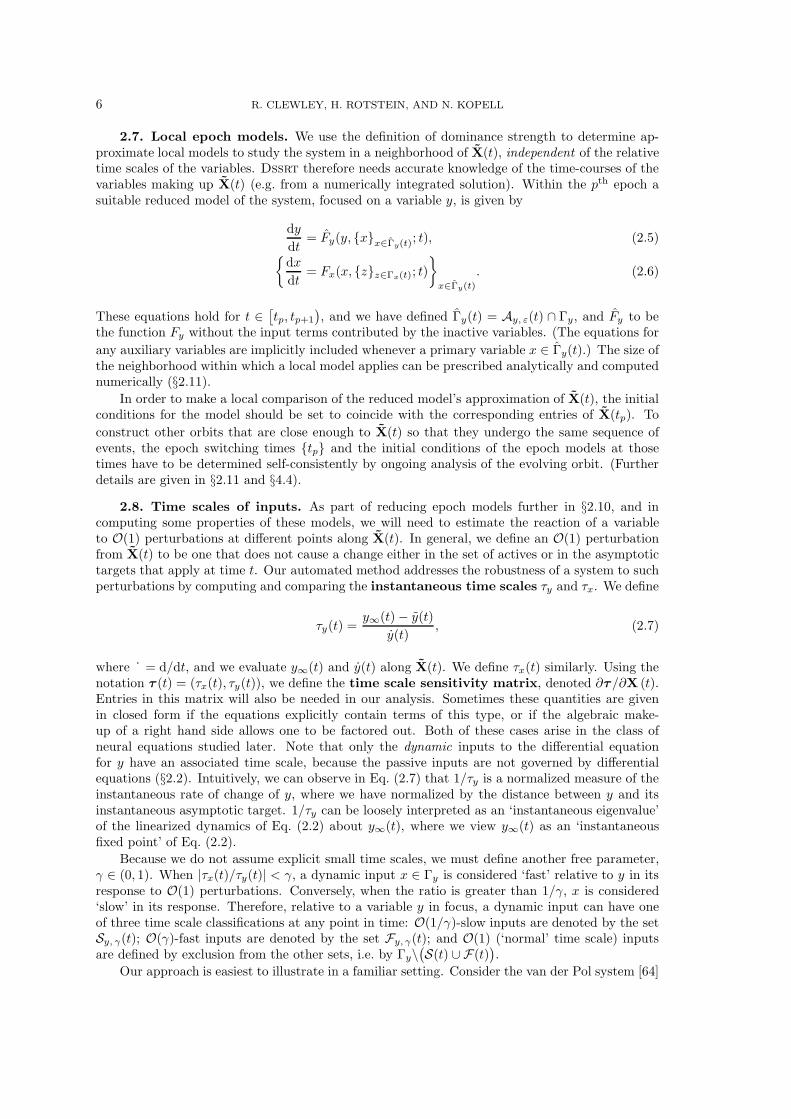
2.8. Time scales of inputs. As part of reducing epoch models further in §2.10, and incomputing some properties of these models, we will need to estimate the reaction of a variableto O(1) perturbations at different points along X(t). In general, we define an O(1) perturbationfrom X(t) to be one that does not cause a change either in the set of actives or in the asymptotictargets that apply at time t. Our automated method addresses the robustness of a system to suchperturbations by computing and comparing the instantaneous time scales τy and τx. We define

τy(t) =y∞(t) − y(t)

y(t), (2.7)

where ˙ = d/dt, and we evaluate y∞(t) and y(t) along X(t). We define τx(t) similarly. Using thenotation τ (t) = (τx(t), τy(t)), we define the time scale sensitivity matrix, denoted ∂τ/∂X (t).Entries in this matrix will also be needed in our analysis. Sometimes these quantities are givenin closed form if the equations explicitly contain terms of this type, or if the algebraic make-up of a right hand side allows one to be factored out. Both of these cases arise in the class ofneural equations studied later. Note that only the dynamic inputs to the differential equationfor y have an associated time scale, because the passive inputs are not governed by differentialequations (§2.2). Intuitively, we can observe in Eq. (2.7) that 1/τy is a normalized measure of theinstantaneous rate of change of y, where we have normalized by the distance between y and itsinstantaneous asymptotic target. 1/τy can be loosely interpreted as an ‘instantaneous eigenvalue’of the linearized dynamics of Eq. (2.2) about y∞(t), where we view y∞(t) as an ‘instantaneousfixed point’ of Eq. (2.2).

Because we do not assume explicit small time scales, we must define another free parameter,γ ∈ (0, 1). When |τx(t)/τy(t)| < γ, a dynamic input x ∈ Γy is considered ‘fast’ relative to y in itsresponse to O(1) perturbations. Conversely, when the ratio is greater than 1/γ, x is considered‘slow’ in its response. Therefore, relative to a variable y in focus, a dynamic input can have oneof three time scale classifications at any point in time: O(1/γ)-slow inputs are denoted by the setSy, γ(t); O(γ)-fast inputs are denoted by the set Fy, γ(t); and O(1) (‘normal’ time scale) inputsare defined by exclusion from the other sets, i.e. by Γy\

(

S(t) ∪ F(t))

.

Our approach is easiest to illustrate in a familiar setting. Consider the van der Pol system [64]


x

y

y = 0x = 0

ta

tb

-1

1

-2 -1 1 2

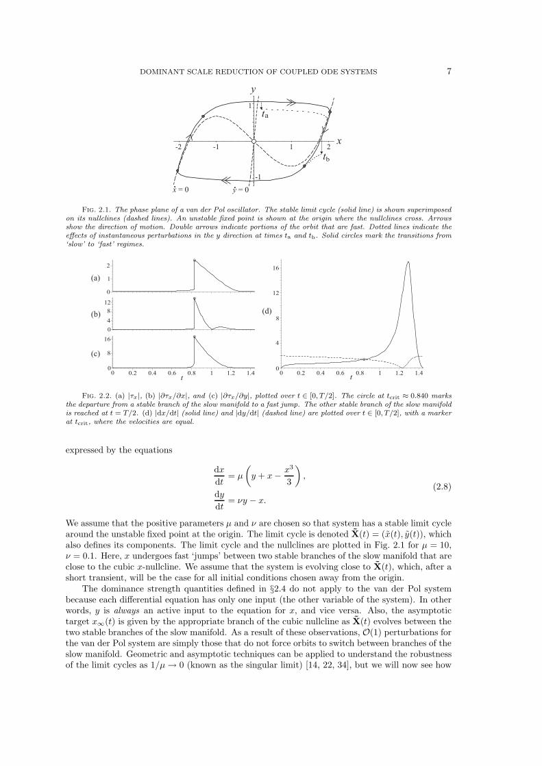
Fig. 2.1. The phase plane of a van der Pol oscillator. The stable limit cycle (solid line) is shown superimposedon its nullclines (dashed lines). An unstable fixed point is shown at the origin where the nullclines cross. Arrowsshow the direction of motion. Double arrows indicate portions of the orbit that are fast. Dotted lines indicate theeffects of instantaneous perturbations in the y direction at times ta and tb. Solid circles mark the transitions from‘slow’ to ‘fast’ regimes.

(a)

(b)

(c)

t

0

1

2

0.2 0.4 0.6 0.8 1 1.2 1.4

0

4

8

12

0

8

16

0

16

8

4

0

t0.2 0.4 0.6 0.8 1 1.2 1.40

(d)12

Fig. 2.2. (a) |τx|, (b) |∂τx/∂x|, and (c) |∂τx/∂y|, plotted over t ∈ [0, T/2]. The circle at tcrit ≈ 0.840 marksthe departure from a stable branch of the slow manifold to a fast jump. The other stable branch of the slow manifoldis reached at t = T/2. (d) |dx/dt| (solid line) and |dy/dt| (dashed line) are plotted over t ∈ [0, T/2], with a markerat tcrit, where the velocities are equal.

expressed by the equations

dx

dt= µ

(

y + x −x3

3

)

,

dy

dt= νy − x.

(2.8)

We assume that the positive parameters µ and ν are chosen so that system has a stable limit cyclearound the unstable fixed point at the origin. The limit cycle is denoted X(t) = (x(t), y(t)), whichalso defines its components. The limit cycle and the nullclines are plotted in Fig. 2.1 for µ = 10,ν = 0.1. Here, x undergoes fast ‘jumps’ between two stable branches of the slow manifold that areclose to the cubic x-nullcline. We assume that the system is evolving close to X(t), which, after ashort transient, will be the case for all initial conditions chosen away from the origin.

The dominance strength quantities defined in §2.4 do not apply to the van der Pol systembecause each differential equation has only one input (the other variable of the system). In otherwords, y is always an active input to the equation for x, and vice versa. Also, the asymptotictarget x∞(t) is given by the appropriate branch of the cubic nullcline as X(t) evolves between thetwo stable branches of the slow manifold. As a result of these observations, O(1) perturbations forthe van der Pol system are simply those that do not force orbits to switch between branches of theslow manifold. Geometric and asymptotic techniques can be applied to understand the robustnessof the limit cycles as 1/µ → 0 (known as the singular limit) [14, 22, 34], but we will now see how


the instantaneous time scale quantities defined in Eq. (2.7) can be used to study robustness awayfrom this limit.

For µ = 10 and ν = 0.1, the period of the limit cycle is T ≈ 2.883. We observe thaty∞ = x/ν = 10x, and we take x∞(t) to be the appropriate branch of the cubic nullcline, dependingon the location of the orbit. We find that τy = −1/ν = −10, so that y∞(t) is in fact a repeller.τx has a complicated (but explicit) form, which is plotted in Fig. 2.2(a). From this plot it is easyto calculate that |τx/τy| ≈ 0 all along the limit cycle, although this ratio rises to nearly 1/4 inthe vicinity of certain ‘critical points’. The critical points are the positions in the cycle when theorbit moves from a slow to a fast manifold, or vice versa. They are marked by closed circles inFig. 2.1. (As 1/µ → 0 the critical points converge to the ‘knees’ of the cubic nullcline.) Away fromthe critical points we also find that the time scale sensitivity matrix entries for τy are identicallyzero, and |∂τx/∂x| and |∂τx/∂y| are shown in Fig. 2.2(b) and (c) to be almost zero. This indicatesthat O(1) perturbations in either variable hardly affect τx, and do not affect τy: in other words,that the separation of time scales is robust. The increased sensitivity of τx near the critical pointat tcrit ≈ 0.840 has decayed by t = 1.2, when the orbit is at approximately (−0.21, 1.05). Thisposition is only a small spatial distance from the critical point relative to the size of the fastjump. The sensitivity of the dynamics in small neighborhoods of the critical points is known tobe important in understanding canard behavior [25, 44].

From measuring the time scale separation around the limit cycle it is reasonable to chooseγ = 1/4, so that Dssrt determines x to be a ‘fast’ variable relative to y over the entire cycle (were-iterate that we mean fast in its response to perturbations, not according to its velocity). Then,by focusing on the variable x, a reasonable model for its dynamics in this situation is to makethe reduction dy/dt = 0, which is analogous to studying the ‘fast system’ in singular perturbationtheory. Conversely, by focusing our method on the slow variable y, we can make the reductionx(t) = x∞(t), which is analogous to studying the ‘slow system’. The sudden changes in τx andits sensitivities quantitatively indicate the shrinking of the neighborhoods around the limit cyclewithin which these reductions apply. These reduction steps are fully described in §2.10 for thegeneral case.

Comparing the time scale quantities can help us avoid the costly computation and comparisonof actual perturbed orbits. Near X(t) we can predict whether variables will remain essentiallyunchanged after a perturbation, or whether they will remain near to their perturbed values. Atechnique to do this is explained in §2.11, but here we take a brief look at the ideas involved usingthe van der Pol example. Consider two scenarios shown in Fig. 2.1, in which we perturb y at atime ta or tb along the limit cycle. The system undergoes a fast jump between stable branches ofthe slow manifold over the time interval (tcrit, T/2). The fast manifold traversed during the jumpis not normally hyperbolic, and locally the vector field is almost horizontal. Thus, a perturbationat time ta ∈ (tcrit, T/2) hardly alters the motion of x, which continues to relax quickly to aslightly perturbed position on the right-hand branch of the slow manifold. By the time the slowmanifold is reached, y has only changed slightly from its perturbed value. The same outcomecan be predicted by observing that the scale separation |τx(ta)| ≪ |τy(ta)| is very robust in a

neighborhood of X(ta). In fact, this observation predicts a qualitatively similar response of thesystem to O(1) perturbations throughout (tcrit, T/2). In contrast, |dx/dt| ≫ |dy/dt| only for asmall part of the jump (Fig. 2.2(d)), because the system is far from the singular limit. Therefore,it is more informative to compare the instantaneous time scales than the velocities in order tounderstand the effect of perturbations, and to characterize the separation of time scales far fromthe singular limit. At tb, the macroscopic motion of the system is dominated by y’s slow dynamics(|dx/dt| < |dy/dt| along the slow manifold), provided it remains close to the limit cycle. However,the reaction of the system to a perturbation in y near the slow manifold is still controlled by thefast response of the x sub-system compared to y, i.e. because |τx| ≪ |τy |. Again, the characteristictime scales allow us to effectively predict the outcome of perturbations. Similar arguments applyif we had instead perturbed x.

2.9. Potentially active inputs. Although a dynamic input may not be active at time t, itis possible that it would have been active if the input variables had taken different values (often,


values that are larger in magnitude). In such a case, these inputs are said to be potentially

active at time t, and belong to the set Py, ε(t). Dssrt determines when this is the case througha constrained maximization of the dominance strengths for the inputs. User-specified boundingintervals for the system’s variables provide the constraints. Although gating variables for physi-ological models are typically designed to vary within the unit interval, a priori bounds are oftenunavailable. In the latter case it is sufficient to specify effective bounds. This can be done byconservatively estimating the extent of the variables’ motion (in a volume containing X(t)) over arange of ‘typical’ initial conditions, external inputs, and perturbations.

The presence of a potentially active input in the r.h.s. of Eq. (2.2) at a given time indicates asensitivity of y’s dynamics to possible fluctuations in the corresponding input variable. Conversely,absence of an input from Py, ε(t) means that the y dynamics are less than O(ε)-dominated by anyvariation in that input at time t. Py, ε(t) provides information about the robustness of orbits inaddition to what we discussed in the previous section. For instance, knowledge of Py, ε(t) overone period of a stable oscillation could be used to determine the necessary timing and amplitudefor effective modulation of the oscillation. In this case, Py, ε(t) would serve a similar purpose toa ‘phase response curve’ [15, 72] or a ‘spike-time response curve’ [3]. During the constructionof orbits via reduced models, Dssrt also tracks potentially active inputs as possible bifurcationparameters or as other sources of regime switching (see §2.11 and §2.12).

2.10. Reduced dynamical regimes. As we will see in the Hodgkin–Huxley example, thesequences of events that our method generates for ODE systems can be highly detailed. Whencompared to the results of standard matched asymptotic analysis of those equations by hand,the epoch sequences may appear to reflect not only intuitively crucial changes in the system, butalso relatively inconsequential ones. As a result, Dssrt incorporates an algorithm that capturessome of the intuition of matched asymptotic analysis for initial-value problems. It simplifies thesequence of P events by consolidating the minor changes to the system and only indicating theneed to change a local model when certain crucial changes in the dynamics occur. The full detailsof the regime determination algorithm’s implementation and use are too lengthy and technical topresent here, so we limit ourselves to a summary of its major elements.

For periodic orbits, the first regime is started at an optimal point in the epoch sequence;otherwise it is started wherever X(t) begins. Epochs are added to the regime incrementally untilthe algorithm decides that circumstances have changed significantly enough that a new regimeshould be started. The set of variables accumulated from all the added epochs prescribes a regimemodel that is focused on y, in the same way as described by Eqs. (2.5)–(2.6) for the epoch models.

There are a variety of controls over the algorithm in Dssrt, but in its simplest form it dictatesthe following. Two epochs that differ only by passive variables are put in the same regime. A newregime is started whenever a fast variable x ∈ Fy, γ joins Ay, ε. A new regime is also started when afast variable leaves Ay, ε, unless the resulting regime would have no dynamic variables remaining inits actives set, and no quasi-static bifurcation variables left to track. Were a regime to be startedin the latter situation, it would be trivial in its dynamics because its reduced equations wouldinvolve only passive input terms. Furthermore, in the absence of dynamic inputs or quasi-staticbifurcation parameters the regime would be devoid of any achievable condition that could end itsreign.

Time scale information was not used in the determination of events or epoch models. Wewill now give a flavor for how the algorithm uses this information to further reduce the dimensionof a regime’s local model. In certain circumstances, fast active variables x ∈ Fy, γ(t) ∩ Ay, ε(t)may be adiabatically eliminated, such that we set x(t) = x∞(t) in the regime model. Onecondition that allows this is if y /∈ Px, ε(t). In this case, y can vary according to Eq. (2.5) in aneighborhood of y(t), and x∞ will change by no more than O(ε) over O(1) time durations. Theadiabatic elimination can proceed provided the regime does not grow too long (i.e. to an O(1/γ)or O(1/ε) length, whichever is shorter). Conversely, if y ∈ Px, ε(t), then y’s evolution may causex∞ to vary substantially from its known value (evaluated along x(t)), or τx may change such thatx /∈ Fy, γ . One of the following cases will apply:

• y /∈ Ax, ε(t). This means that there is a neighborhood around y(t) within which x will


remain O(ε)-close to x(t). Within this neighborhood, x∞ can be reasonably estimated byits value evaluated along x(t), provided the regime does not grow too long. Additionally,if |∂τx/∂y| is small along x(t), then any changes induced in τx in the neighborhood aroundy(t) will occur much more slowly than the attraction of x to its instantaneous asymptotictarget, and we can proceed with the elimination. The neighborhood can be explicitlycalculated.

• y ∈ Ax, ε(t). This means that O(1) changes in y will cause O(1) changes in x, and we donot have an easy way to estimate a neighborhood within which the adiabatic eliminationwill be accurate. Therefore, we do not proceed with the elimination.

Slow active variables in Sy, γ(t) that also have weak time scale sensitivity to y are replaced inthe regime with an appropriate constant value, provided the regime does not become too long. Theconstant value is determined self-consistently from looking at neighboring regimes. Consistencychecks similar to those needed for the adiabatic eliminations are required.

The result of this process is a number R ≤ P of consolidated events, defining R − 1 reduced

dynamical regimes. The regimes tell a concise story of the most important interactions betweenvariables evolving in a neighborhood of X(t), from the perspective of a single variable. Due tothe consolidation of the events, the regimes are delimited by time intervals [tr, tr+1), where r =1, . . . , R−1, and {tr} ⊆ {tp}. The checks required for determining the time-scale based reductionsform part of the validity conditions discussed in the next section.

2.11. Regime validity conditions and robustness. As well as studying perturbationproperties of X(t) relative to a variable y, we can use the regime models to construct new orbitsclose to X(t). Care must be taken to ensure that such orbits accurately represent true orbits ofthe full system (at least qualitatively) by the continual verification of various validity conditions.These conditions can be posed as tests for zero crossings in algebraic functions of the system’svariables, their dominance strengths, their time scales, and so forth. These augment the differentialequations for the regime to yield a set of differential-algebraic equations for the regime [62]. Thisalso means that the collection of reduced models can be viewed as a hybrid dynamical system [65].We consider an (N + 1)-dimensional volume D ≡ D(ε, γ) ⊂ R

N × R around X(t), which is thelargest volume within which the validity conditions for constructed orbits hold true. We refer tothis volume as the local domain of validity (d.o.v.) for the reduced regimes. Self-consistencyalso requires that all orbits constructed during the rth regime lie entirely within D|t∈[tr,tr+1). Wecan make use of our explicit knowledge of the equations and the values of ε and γ to calculate D.This validation process is asymptotically accurate, i.e. it can prescribe the d.o.v. precisely only inthe limit of vanishingly small ε and γ. Thus, ε and γ determine error tolerances for the accuracyof the computed d.o.v. Before describing Dssrt’s method of estimating the d.o.v., we describethe three types of regime validity condition in detail.

(1) A regime becomes invalid if the sets of actives or the time scale classifications computedalong constructed orbits (or as a result of perturbations from the reference orbit X(t)) deviatesubstantially from those determined for X(t). Therefore, a deviation of this kind must not occurduring the time evolution of the variables that are explicitly modeled in the regime.

(2) In the full ODE system given by Eq. (2.1), the motion of the variables explicitly modeledin a reduced dynamical regime may both affect and depend on the motion of the coupled variablesthat are not modeled. Thus, to have confidence in the accuracy of the regime model’s dynamics,we must verify that the regime’s assumptions are not invalidated by virtue of implied changes inthe un-modeled variables of the system. We define a shadowing error to occur if the neglectedfeedback from the un-modeled dynamics causes enough error to accumulate in the constructionof an orbit such that the regime’s assumptions about Ay, ε, Fy, γ , and Sy, γ become invalidated.Shadowing errors are subtle and hard to detect because the reduced model may continue toproduce plausible-looking orbits, whereas the full system starting from the same initial conditionscould have significantly diverged. Of course, it is not generally desirable to compute the orbits ofthe full system in order to validate those constructed using a reduced model. An existing bodyof literature, concerning the error analysis of numerical solutions of ODEs, develops theories ofshadowing more rigorously [29, 53]. We return to the practical implementation of conditions (1)


and (2) in Dssrt shortly.

(3) The local models of consecutive regimes involve different constituent variables (usuallywith some overlap). This forces us to address the validity of passing the projection of the fullN -dimensional system between the low-dimensional models at discrete time events. Therefore,Dssrt must ensure that the correct ‘structural’ changes occur in the system as a constructedorbit progresses beyond the remit of the current regime, in comparison to the known changesalong the reference orbit. If such a condition fails, then Dssrt will not know which regime tohand over control to. This is especially relevant to regime transitions in which the local modelgains variables, since a previously inactive (i.e., not modeled) variable needs to have an appropriateinitial condition after the transition. The regime determination algorithm attempts to determinewhich slowly changing or potentially active variables (in Py, ε) need to be tracked in order forDssrt to accurately predict a transition into the next regime. These are known as the quasi-

static bifurcation parameters for the regime. The magnitude of these variables must be trackedover the course of the preceding regime because they may be crucial in causing the local modelto undergo a bifurcation (§2.12) or a change in time scale relationships. Such events signal thatcontrol of the dynamics should be passed to the next regime of the sequence generated for thereference orbit. A concrete example using this condition is given at the end of §4.4.

The remainder of this section is an overview of the most important factors used in the self-consistency checks implemented by Dssrt. To verify conditions (1) and (2) in practice, Dssrt

requires estimates of the time scales and asymptotic targets of the variables in a neighborhood ofthe reference orbit. Together with their sensitivities to small variation in the un-modeled variables,these quantities can provide Dssrt with enough confidence that the positive feedback loops whichcause the shadowing errors are unlikely. A simple example of testing these conditions was given in§2.8 for a van der Pol system. Also, tests relating to changes in the system’s time scale relationshipswere discussed in more detail at the end of the previous section. Currently, Dssrt does not fullyimplement these tests. Instead, Dssrt estimates the d.o.v. in the following conservative way.

Over a high-resolution set of sample times {ts} taken over the duration of the reference orbit,a variable y of the full system is perturbed from its values y(ts) to values we denote by y∗(ts).If the set of actives Ay, ε(ts) and the time scale relationships given by Fy, γ(ts) and Sy, γ(ts) arenot changed by a perturbation at ts, then y∗ is included in the restriction of the d.o.v. to they-direction, denoted D|y , at the sample time ts. Dssrt performs a bisection search to find themaximally large perturbations y∗ from y(t) that can be included in D|y.

The values of the dominance strengths will remain approximately unchanged under these per-turbations provided the input variables to the differential equation for y do not change significantly.Herein lies the benefit of defining the dominance strengths in Eq. 2.4 for Ψ to be independent ofthe instantaneous value of y, and dependent instead on y∞. The position of y∞ depends directlyon the values of the inputs in Γy only, and not on y. Therefore it is sufficient to verify three con-ditions on the inputs to Fy in order that the actives set remains unchanged after a perturbationy(ts) → y∗(ts):

• Fast inputs x ∈ Fy, γ(ts), which almost instantaneously reach perturbed values x∗ ≈x∞(y∗), must not cause a change in Ay, ε(ts) when it is recomputed using the perturbedvalues x∗. This is checked for both the active and the inactive inputs, to avoid introducinga shadowing error. Furthermore, a global check can be made to ensure that these changesin x do not change any Az, ε(ts) in the system, for z 6= x.

• Slow inputs x ∈ Sy, γ are assumed not to change at all under the perturbation, on thelocal time scale of y’s evolution. Therefore, these will not impact the dominance strengthsΨx under the perturbation.

• The remaining dynamic inputs x ∈ Γy have an O(1) time scale (i.e. are considered neitherfast nor slow). How x responds to the perturbation in y depends on whether y is currentlyin its active set, Ax, ε (among other things). If this is so, then y∞ must be re-evaluatedwith the orbits x(t) replaced with new estimates for the x(t) following the perturbation.In the absence of a more sophisticated method to ensure that these estimates will be safe,we assume the worst-case scenario: namely, that x is as far from x(t) as possible. This


means we estimate x(t) = x∞(t), evaluated at y∗. The actives set for y can then bere-evaluated using the perturbed y∞, and tested for change. If y /∈ Ax, ε, then Dssrt

estimates that x will not change significantly on the local time scale.Finally, Dssrt tests whether the inputs have changed their membership in the sets Sy, γ(ts)

and Fy, γ(ts), by re-determining these sets using the τy and τx values evaluated at the perturbedvalues y∗ and x∗.

2.12. Bifurcations in the regime models. Reduced regimes can be studied for the lossof stability of any fixed points that exist in the local model, as parameters change (including thequasi-static parameters defined earlier). The loss of stability of periodic orbits requires globalarguments which are not developed here, although the breaking of certain types of regime validitycondition could be used as an indication that a constructed or perturbed orbit is diverging froma reference limit cycle orbit. As a parameter is varied, a sign change in τx indicates that x∞ hasswitched between being an attractor and a repeller. This is conceptually similar to the occurrenceof a local bifurcation, when x∞ is viewed as an ‘instantaneous fixed point’ and τx is interpretedas an associated ‘instantaneous eigenvalue’ (§2.8).

The structure of the regimes could also be used to set up a more conventional bifurcationanalysis, either by hand, such as that undertaken in [57], or using a numerical continuation softwarepackage such as Auto [13]. Examples of local bifurcation analysis using the regimes are given in§4.4 for a Hodgkin–Huxley model neuron.

3. Application to a Hodgkin–Huxley model neuron.

3.1. A synaptically-driven Hodgkin–Huxley neuron. The example ODE system stud-ied for the remainder of this paper models a Hodgkin–Huxley-type neuron with a single inhibitorychemical synapse as an external input. In a traditional form of notation, the system of equa-tions consists of the following current-balance equation for the membrane potential V , and theassociated equations for the non-dimensional activation variables x(t) ∈ [0, 1]:

CdV

dt= Iionic (V, m, h, n) + Iexternal (V, t)

≡ gmm3h (Vm − V ) + gnn4 (Vn − V )

+ gl (Vl − V ) + gss (Vs − V ) + Ib, (3.1)

τx(V )dx

dt= x∞(V ) − x, x = m, h, n, (3.2)

where we define the internal ionic current Iionic = gmm3h (Vm − V )+ gnn4 (Vn − V )+ gl (Vl − V ),the sum of a fast sodium current, a fast potassium current, and a ‘leak’ current. m represents thesodium channel activation in the cell membrane, h is the sodium channel inactivation, and n isthe potassium channel activation. The external current Iexternal = gss (Vs − V ) + Ib is the sumof a synaptic input and a fixed bias current. Iionic is the source of the membrane’s excitability;in other words, its ability to generate ‘action potential’ spikes. The timing of spikes is dictatedby Iexternal when all other parameters are fixed. The coefficients gx represent the maximumconductances of the ionic channels. Each activation variable has a voltage-dependent time scaleτx(V ) and instantaneous asymptotic target x∞(V ), which are explicitly known functions. Thestandard choice of C = 1 µF/cm2 for this type of cell leads us to drop the capacitance parameterfrom our equations hereafter. In this example, the values for all the parameters and functionsτx(V ), x∞(V ) are fixed, and are detailed in the Appendix.

The synaptic drive input has a gating variable s(t) ∈ [0, 1], which is the fifth variable in thesystem. It has a similar form to an activation variable:

ds

dt= αΘ (Vpre(t)) (1 − s) − βs, (3.3)

where Θ(Vpre) = (1 + tanh (Vpre/4)) /2 is a smooth step function, and α and β control the riseand fall times of an inhibitory pulse. Here, the inhibitory pulse is stimulated by a pre-synaptic


spike from a externally applied, time-varying input, Vpre(t) (defined in the Appendix), that mimicsthe regular spiking of another cell. By choosing the reversal potential Vs in Eq. (3.1) to be belowthe threshold of spike initiation, this synaptic input is inhibitory.

3.2. Inputs to the voltage equation. We take several steps in order to standardize ournotation and apply the dominant scale method. Firstly, we ignore the physiological distinction of‘ionic’ versus ‘external’ currents to the neuron. We define n = gn, l = gl, s = gs, and b = Ib.These re-labelings are superficial, but we make the leak and bias current terms consistent with thenotation of other inputs by formally including the gating ‘variables’ l ≡ 1 and b ≡ 1, respectively.For the sodium conductance, we consider m to be the primary variable and h the auxiliary (i.e. amodulator of m). As a result, we will not analyze the effect of perturbations in h. This choice ofprimary variable is satisfactory (although somewhat arbitrary) because both variables depend onlyon V , and not on any external sources. We therefore define the time-varying maximal conductancem = m(t) = gm h(t), and henceforth write the sodium current mm3(Vm − V ).

It is appropriate to consider all additive terms that contribute to the r.h.s. of Eq. (3.1) as inputsbecause each term has a distinct physiological interpretation. Thus, for the voltage equation,the five input terms are the sodium activation/inactivation term mm3 (Vm − V ), the potassiumactivation term nn4 (Vn − V ), the leak term ll (Vl − V ), the synaptic term ss (Vs − V ), and thebias current bb. The five corresponding variables form the set of inputs ΓV = {m, n, l, b, s}, wherewe include only primary variables.

The variables m, h, n, and s, are governed by their own differential equations, and so theinputs to Eq. (3.1) that involve them are dynamic inputs. The leak and bias current inputs arepassive. In addition to this distinction, we note that an input term is either explicitly dependent onV , having the form xxqx (Vx − V ), or independent, having the form xxqx . Here, x is the maximalvalue of the input (time-varying in the presence of auxiliary variables), x ≡ x(t) ∈ [0, 1] determinesthe time-course of the input, and qx is a positive integer. Inputs of the first type belong to Γ1,and those of the second type belong to Γ2 = ΓV \Γ1.

Using these definitions, a simple algebraic manipulation shows that the voltage and synapticequations have the same form as the activation variables:

τV

(

{x}x∈Γ1

)dV

dt= V∞

(

{x}x∈ΓV

)

− V , (3.4)

τs(Vpre)ds

dt= s∞(Vpre) − s, (3.5)

where

1/τV = mm3 + nn4 + ll + ss,

V∞ =(

mm3Vm + nn4Vn + lVl + ssVs + bb)

τV ,

τs = αΘ (Vpre) + β,

s∞ = αΘ (Vpre) /(

αΘ (Vpre) + β)

.

3.3. Conditionally linear ODEs. As a result of the re-arrangement of the HH system, wesee that each equation of the system explicitly has the form τxx = x∞ − x, where x = V, m, n, h,or s. τx and x∞ may be functions of external inputs or other variables in the system (but not ofx). Also, each x∞(t) is unique. These are general properties of Hodgkin–Huxley-type models, dueto the conditional linearity of the equations, i.e. that each differential equation is linear in its owndependent variable, when the values of the other variables appearing in the equation are known.The conditional linearity of the HH model simplifies various computations and checks requiredby our method. For instance, because the characteristic time scale coefficients τx are explicitlyknown functions that are strictly positive, we observe that the HH system is dissipative at alltimes. Another beneficial consequence of conditional linearity is that each variable x is attractedto x∞(t) exponentially, which is a stronger property than the normal hyperbolicity that we require.


t

s

n

V

h

m

Fig. 3.1. The limit cycle for the HH system projected in its 5 constituent dimensions.

3.4. Dominance strengths. In this model of a single neuron we consider only the influenceof inputs on the V dynamics, because the other equations have only one input. There are two typesof influence that inputs have on the differential equation for V . Inputs in Γ1 affect both the V∞

and τV values, whereas those in Γ2 affect only V∞. Because of the conditional linearity of the HHequations, and the positivity of the activation variables x, their time scales τx, and their powersqx, the definition of dominance strength in Eq. (2.4) reduces to a form that is computationallymore practical.

Ψx(t) =

{

τV (t) qxxxqx (t) |Vx − V∞(t)| if x ∈ Γ1,

τV (t) qxxxqx (t) if x ∈ Γ2.(3.6)

We see that for Γ1 inputs, Ψx resembles the input term for x (in physiological terms, this wouldbe the current through the channel associated with x) except that V∞ replaces V , and there isan additional multiplication by τV . For Γ2 our definition coincides with the associated input term(modulo the factor of τV ).

3.5. Local epoch models. For any initial condition, the HH system quickly settles to alimit cycle (shown in Fig. 3.1), having the same period as the inhibitory driving signal, namely50 ms (hereafter denoted T ). This limit cycle, and a neighborhood around it, will be the focus ofthe subsequent analysis, and we denote it X(t), where X = (V , m, n, h, s) defines its components.

Focusing on the voltage V , the epoch model in a neighborhood of X(t) over t ∈[

tp, tp+1

)

isgiven by

dV

dt=

∑

x∈Γ1(t)

xxqx (Vx − V ) +∑

x∈Γ2(t)

xxqx , (3.7)

{

dx

dt=

1

τx(x∞ − x)

}

x∈(

Γ1∪Γ2

)

(t)

, (3.8)

where Γ1(t) = AV, ε(t) ∩ Γ1, Γ2(t) = AV, ε(t) ∩ Γ2, and the equation for the auxiliary variable h is

also included whenever m ∈ Γ1(t).Using ε = 2/5 in Dssrt we obtained an epoch sequence of length 12. The sequence is tabulated

in the first three columns of Table 3.1. (Values ε ∈ [1/5, 1/3] have yielded reasonable results for the


Epoch Time interval AV, ε PV, ε

1 [00.00, 00.03) s, b, l m, n2 [00.03, 28.26) s, b m, n3 [28.26, 29.04) s, b, l m, n4 [29.04, 33.57) m, s, b, l n5 [33.57, 34.59) m, b, l s, n6 [34.59, 34.77) m, l s, n7 [34.77, 36.87) m s, n8 [36.87, 37.62) m, n9 [37.62, 38.79) n m10 [38.79, 39.00) n, b m, s11 [39.00, 39.21) n, b, l m, s12 [39.21, 49.98) b, l m, n, s

Table 3.1

The epoch sequence determined by Dssrt for the limit cycle oscillation, with period T = 50ms. Time intervalsare measured relative to the onset of an inhibitory pulse at t = 200 ms. The size of the numerical integration stepand the re-sampling done by Dssrt caused the final interval to stop short of precisely t = T .

-100

-80

-60

-40

-20

0

20

40

250200 210 220 230 240

{ }l, b

{ }s, l, b { }s, l, b, m

{ }m, n

{ }m, l, b

{ }n, l, b

Regime I

Fig. 3.2. One period in V (t), with V∞(t) (dotted line). The reduced set of regimes along the limit cycle areshown below the graph with their associated set of actives AV, ε.

neural models we have studied so far.) A temporal resolution of 0.03 ms was used to analyze thenumerically integrated orbit (computed using the Runge–Kutta scheme at a time step of 0.01 ms).This resolution accounts for the slight discrepancy of 0.02 ms in the total length of the regimesmaking up the cycle from the known driving period of 50 ms, despite having used initial conditionsfor the system very close to the periodic orbit. The temporal resolution of Dssrt’s analysis canbe altered by the user to match the smallest time scales of the events in the dynamics.

3.6. Potentially active inputs. Another consequence of conditional linearity aids the cal-culation of potentially active inputs. For such systems, the value of the input variable thatmaximizes its dominance strength can be determined explicitly as a function of the system state.The turning-point condition dΨx/dx = 0 can be solved explicitly from the r.h.s. of Eq. (3.6), andDssrt takes the maximum value of the dominance strength evaluated at the solutions to thisturning point condition and at the end points of the assumed bounds for the variable x (i.e. 0and 1 for the activation variables in the HH system). This approach avoids the need to calculatethe second derivative of the dominance strength to check for a maximum. The potentially activevariables in each epoch along the periodic orbit X(t) for the HH system are tabulated in the finalcolumn of Table 3.1.


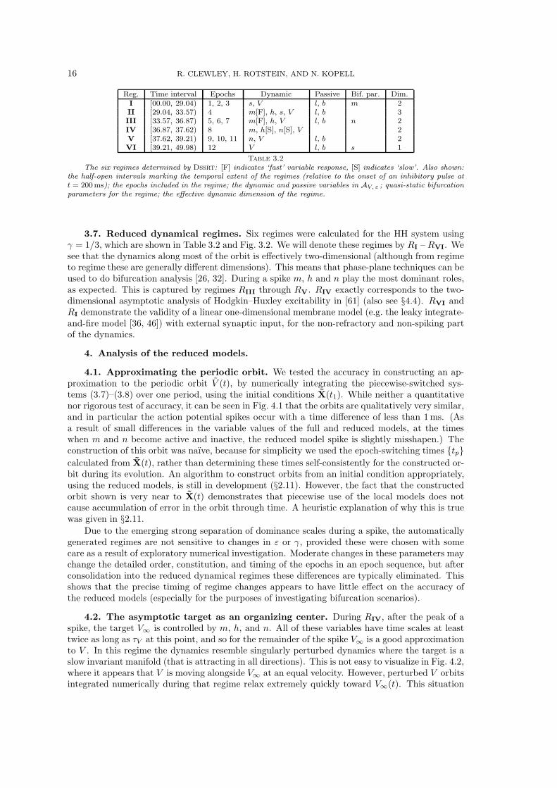
Reg. Time interval Epochs Dynamic Passive Bif. par. Dim.I [00.00, 29.04) 1, 2, 3 s, V l, b m 2II [29.04, 33.57) 4 m[F], h, s, V l, b 3III [33.57, 36.87) 5, 6, 7 m[F], h, V l, b n 2IV [36.87, 37.62) 8 m, h[S], n[S], V 2V [37.62, 39.21) 9, 10, 11 n, V l, b 2VI [39.21, 49.98) 12 V l, b s 1

Table 3.2

The six regimes determined by Dssrt: [F] indicates ‘fast’ variable response, [S] indicates ‘slow’. Also shown:the half-open intervals marking the temporal extent of the regimes (relative to the onset of an inhibitory pulse att = 200ms); the epochs included in the regime; the dynamic and passive variables in AV, ε ; quasi-static bifurcationparameters for the regime; the effective dynamic dimension of the regime.

3.7. Reduced dynamical regimes. Six regimes were calculated for the HH system usingγ = 1/3, which are shown in Table 3.2 and Fig. 3.2. We will denote these regimes by RI – RVI. Wesee that the dynamics along most of the orbit is effectively two-dimensional (although from regimeto regime these are generally different dimensions). This means that phase-plane techniques can beused to do bifurcation analysis [26, 32]. During a spike m, h and n play the most dominant roles,as expected. This is captured by regimes RIII through RV. RIV exactly corresponds to the two-dimensional asymptotic analysis of Hodgkin–Huxley excitability in [61] (also see §4.4). RVI andRI demonstrate the validity of a linear one-dimensional membrane model (e.g. the leaky integrate-and-fire model [36, 46]) with external synaptic input, for the non-refractory and non-spiking partof the dynamics.

4. Analysis of the reduced models.

4.1. Approximating the periodic orbit. We tested the accuracy in constructing an ap-proximation to the periodic orbit V (t), by numerically integrating the piecewise-switched sys-tems (3.7)–(3.8) over one period, using the initial conditions X(t1). While neither a quantitativenor rigorous test of accuracy, it can be seen in Fig. 4.1 that the orbits are qualitatively very similar,and in particular the action potential spikes occur with a time difference of less than 1 ms. (Asa result of small differences in the variable values of the full and reduced models, at the timeswhen m and n become active and inactive, the reduced model spike is slightly misshapen.) Theconstruction of this orbit was naıve, because for simplicity we used the epoch-switching times {tp}

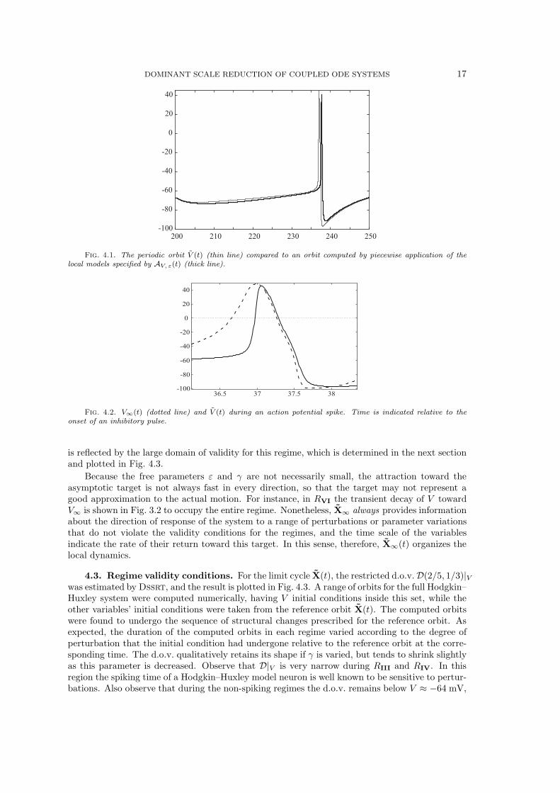
calculated from X(t), rather than determining these times self-consistently for the constructed or-bit during its evolution. An algorithm to construct orbits from an initial condition appropriately,using the reduced models, is still in development (§2.11). However, the fact that the constructedorbit shown is very near to X(t) demonstrates that piecewise use of the local models does notcause accumulation of error in the orbit through time. A heuristic explanation of why this is truewas given in §2.11.

Due to the emerging strong separation of dominance scales during a spike, the automaticallygenerated regimes are not sensitive to changes in ε or γ, provided these were chosen with somecare as a result of exploratory numerical investigation. Moderate changes in these parameters maychange the detailed order, constitution, and timing of the epochs in an epoch sequence, but afterconsolidation into the reduced dynamical regimes these differences are typically eliminated. Thisshows that the precise timing of regime changes appears to have little effect on the accuracy ofthe reduced models (especially for the purposes of investigating bifurcation scenarios).

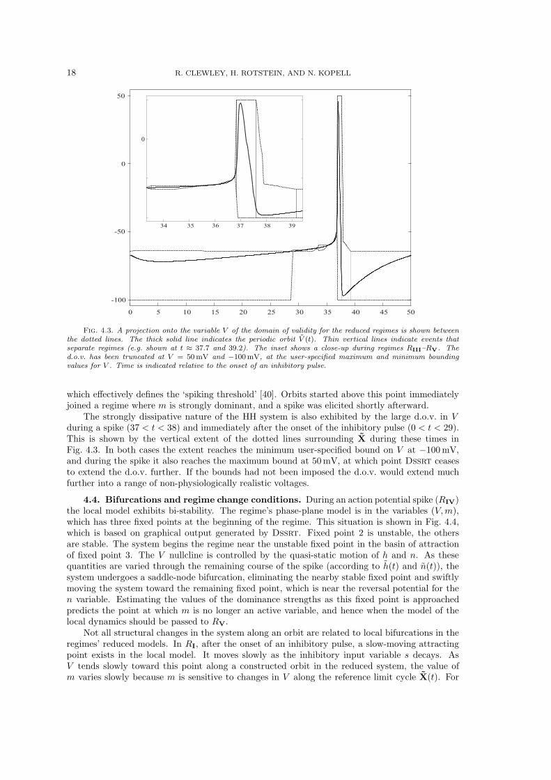
4.2. The asymptotic target as an organizing center. During RIV, after the peak of aspike, the target V∞ is controlled by m, h, and n. All of these variables have time scales at leasttwice as long as τV at this point, and so for the remainder of the spike V∞ is a good approximationto V . In this regime the dynamics resemble singularly perturbed dynamics where the target is aslow invariant manifold (that is attracting in all directions). This is not easy to visualize in Fig. 4.2,where it appears that V is moving alongside V∞ at an equal velocity. However, perturbed V orbitsintegrated numerically during that regime relax extremely quickly toward V∞(t). This situation


-100

-80

-60

-40

-20

0

20

40

200 210 220 230 240 250

Fig. 4.1. The periodic orbit V (t) (thin line) compared to an orbit computed by piecewise application of thelocal models specified by AV, ε(t) (thick line).

-100

-80

-60

-40

-20

0

20

40

36.5 37 37.5 38

Fig. 4.2. V∞(t) (dotted line) and V (t) during an action potential spike. Time is indicated relative to theonset of an inhibitory pulse.

is reflected by the large domain of validity for this regime, which is determined in the next sectionand plotted in Fig. 4.3.

Because the free parameters ε and γ are not necessarily small, the attraction toward theasymptotic target is not always fast in every direction, so that the target may not represent agood approximation to the actual motion. For instance, in RVI the transient decay of V towardV∞ is shown in Fig. 3.2 to occupy the entire regime. Nonetheless, X∞ always provides informationabout the direction of response of the system to a range of perturbations or parameter variationsthat do not violate the validity conditions for the regimes, and the time scale of the variablesindicate the rate of their return toward this target. In this sense, therefore, X∞(t) organizes thelocal dynamics.

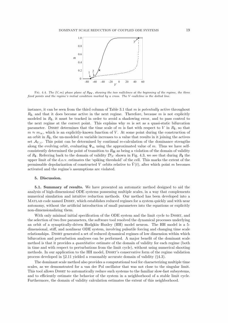
4.3. Regime validity conditions. For the limit cycle X(t), the restricted d.o.v. D(2/5, 1/3)|Vwas estimated by Dssrt, and the result is plotted in Fig. 4.3. A range of orbits for the full Hodgkin–Huxley system were computed numerically, having V initial conditions inside this set, while theother variables’ initial conditions were taken from the reference orbit X(t). The computed orbitswere found to undergo the sequence of structural changes prescribed for the reference orbit. Asexpected, the duration of the computed orbits in each regime varied according to the degree ofperturbation that the initial condition had undergone relative to the reference orbit at the corre-sponding time. The d.o.v. qualitatively retains its shape if γ is varied, but tends to shrink slightlyas this parameter is decreased. Observe that D|V is very narrow during RIII and RIV. In thisregion the spiking time of a Hodgkin–Huxley model neuron is well known to be sensitive to pertur-bations. Also observe that during the non-spiking regimes the d.o.v. remains below V ≈ −64 mV,


0 5 10 15 20 25 30 35 40 45

-100

-50

0

50

50

34 35 36 37 38 39

0

Fig. 4.3. A projection onto the variable V of the domain of validity for the reduced regimes is shown betweenthe dotted lines. The thick solid line indicates the periodic orbit V (t). Thin vertical lines indicate events thatseparate regimes (e.g. shown at t ≈ 37.7 and 39.2). The inset shows a close-up during regimes RIII–RV. Thed.o.v. has been truncated at V = 50 mV and −100mV, at the user-specified maximum and minimum boundingvalues for V . Time is indicated relative to the onset of an inhibitory pulse.

which effectively defines the ‘spiking threshold’ [40]. Orbits started above this point immediatelyjoined a regime where m is strongly dominant, and a spike was elicited shortly afterward.

The strongly dissipative nature of the HH system is also exhibited by the large d.o.v. in Vduring a spike (37 < t < 38) and immediately after the onset of the inhibitory pulse (0 < t < 29).This is shown by the vertical extent of the dotted lines surrounding X during these times inFig. 4.3. In both cases the extent reaches the minimum user-specified bound on V at −100 mV,and during the spike it also reaches the maximum bound at 50 mV, at which point Dssrt ceasesto extend the d.o.v. further. If the bounds had not been imposed the d.o.v. would extend muchfurther into a range of non-physiologically realistic voltages.

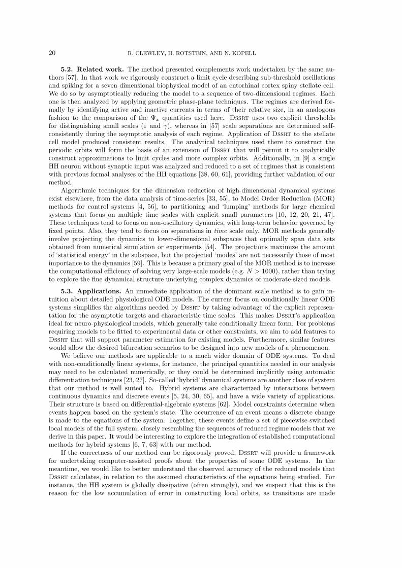
4.4. Bifurcations and regime change conditions. During an action potential spike (RIV)the local model exhibits bi-stability. The regime’s phase-plane model is in the variables (V, m),which has three fixed points at the beginning of the regime. This situation is shown in Fig. 4.4,which is based on graphical output generated by Dssrt. Fixed point 2 is unstable, the othersare stable. The system begins the regime near the unstable fixed point in the basin of attractionof fixed point 3. The V nullcline is controlled by the quasi-static motion of h and n. As thesequantities are varied through the remaining course of the spike (according to h(t) and n(t)), thesystem undergoes a saddle-node bifurcation, eliminating the nearby stable fixed point and swiftlymoving the system toward the remaining fixed point, which is near the reversal potential for then variable. Estimating the values of the dominance strengths as this fixed point is approachedpredicts the point at which m is no longer an active variable, and hence when the model of thelocal dynamics should be passed to RV.

Not all structural changes in the system along an orbit are related to local bifurcations in theregimes’ reduced models. In RI, after the onset of an inhibitory pulse, a slow-moving attractingpoint exists in the local model. It moves slowly as the inhibitory input variable s decays. AsV tends slowly toward this point along a constructed orbit in the reduced system, the value ofm varies slowly because m is sensitive to changes in V along the reference limit cycle X(t). For


0

0.2

0.4

0.6

0.8

1.0

-80 -60 -40 -20 0 20 40 60V

m

1 2

3

x

Fig. 4.4. The (V, m) phase plane of RIV, showing the two nullclines at the beginning of the regime, the threefixed points and the regime’s initial condition marked by a cross. The V -nullcline is the dotted line.

instance, it can be seen from the third column of Table 3.1 that m is potentially active throughoutRI, and that it does become active in the next regime. Therefore, because m is not explicitlymodeled in RI, it must be tracked in order to avoid a shadowing error, and to pass control tothe next regime at the correct point. This explains why m is set as a quasi-static bifurcationparameter. Dssrt determines that the time scale of m is fast with respect to V in RI, so thatm ≈ m∞, which is an explicitly-known function of V . At some point during the construction ofan orbit in RI, the un-modeled m variable increases to a value that results in it joining the activesset AV, ε. This point can be determined by continual re-calculation of the dominance strengthsalong the evolving orbit, evaluating Ψm using the approximated value of m. Thus we have self-consistently determined the point of transition to RII as being a violation of the domain of validityof RI. Referring back to the domain of validity D|V shown in Fig. 4.3, we see that during RI theupper limit of the d.o.v. estimates the ‘spiking threshold’ of the cell. This marks the extent of thepermissable depolarization of constructed V orbits relative to V (t), after which point m becomesactivated and the regime’s assumptions are violated.

5. Discussion.

5.1. Summary of results. We have presented an automatic method designed to aid theanalysis of high-dimensional ODE systems possessing multiple scales, in a way that complementsnumerical simulation and intuitive reduction methods. Our method has been developed into aMatlab code named Dssrt, which establishes reduced regimes for a system quickly and with nearautonomy, without the artificial introduction of small parameters into the equations or explicitlynon-dimensionalizing them.

With only minimal initial specification of the ODE system and the limit cycle to Dssrt, andthe selection of two free parameters, the software tool resolved the dynamical processes underlyingan orbit of a synaptically-driven Hodgkin–Huxley (HH) model neuron. The HH model is a 5-dimensional, stiff, and nonlinear ODE system, involving pulsatile forcing and changing time scalerelationships. Dssrt generated a set of reduced dynamical regimes of low dimension within whichbifurcation and perturbation analyses can be performed. A major benefit of the dominant scalemethod is that it provides a quantitative estimate of the domain of validity for each regime (bothin time and with respect to perturbations from the limit cycle), without using numerical shootingmethods. In our application to the HH model, Dssrt’s conservative form of the regime validationprocess developed in §2.11 yielded a reasonably accurate domain of validity (§4.3).

The dominant scale method also provides a computational tool for characterizing multiple timescales, as we demonstrated for a van der Pol oscillator that was not close to the singular limit.This tool allows Dssrt to automatically reduce such systems to the familiar slow-fast subsystems,and to efficiently estimate the behavior of the system in a neighborhood of a stable limit cycle.Furthermore, the domain of validity calculation estimates the extent of this neighborhood.


5.2. Related work. The method presented complements work undertaken by the same au-thors [57]. In that work we rigorously construct a limit cycle describing sub-threshold oscillationsand spiking for a seven-dimensional biophysical model of an entorhinal cortex spiny stellate cell.We do so by asymptotically reducing the model to a sequence of two-dimensional regimes. Eachone is then analyzed by applying geometric phase-plane techniques. The regimes are derived for-mally by identifying active and inactive currents in terms of their relative size, in an analogousfashion to the comparison of the Ψx quantities used here. Dssrt uses two explicit thresholdsfor distinguishing small scales (ε and γ), whereas in [57] scale separations are determined self-consistently during the asymptotic analysis of each regime. Application of Dssrt to the stellatecell model produced consistent results. The analytical techniques used there to construct theperiodic orbits will form the basis of an extension of Dssrt that will permit it to analyticallyconstruct approximations to limit cycles and more complex orbits. Additionally, in [9] a singleHH neuron without synaptic input was analyzed and reduced to a set of regimes that is consistentwith previous formal analyses of the HH equations [38, 60, 61], providing further validation of ourmethod.

Algorithmic techniques for the dimension reduction of high-dimensional dynamical systemsexist elsewhere, from the data analysis of time-series [33, 55], to Model Order Reduction (MOR)methods for control systems [4, 56], to partitioning and ‘lumping’ methods for large chemicalsystems that focus on multiple time scales with explicit small parameters [10, 12, 20, 21, 47].These techniques tend to focus on non-oscillatory dynamics, with long-term behavior governed byfixed points. Also, they tend to focus on separations in time scale only. MOR methods generallyinvolve projecting the dynamics to lower-dimensional subspaces that optimally span data setsobtained from numerical simulation or experiments [54]. The projections maximize the amountof ‘statistical energy’ in the subspace, but the projected ‘modes’ are not necessarily those of mostimportance to the dynamics [59]. This is because a primary goal of the MOR method is to increasethe computational efficiency of solving very large-scale models (e.g. N > 1000), rather than tryingto explore the fine dynamical structure underlying complex dynamics of moderate-sized models.

5.3. Applications. An immediate application of the dominant scale method is to gain in-tuition about detailed physiological ODE models. The current focus on conditionally linear ODEsystems simplifies the algorithms needed by Dssrt by taking advantage of the explicit represen-tation for the asymptotic targets and characteristic time scales. This makes Dssrt’s applicationideal for neuro-physiological models, which generally take conditionally linear form. For problemsrequiring models to be fitted to experimental data or other constraints, we aim to add features toDssrt that will support parameter estimation for existing models. Furthermore, similar featureswould allow the desired bifurcation scenarios to be designed into new models of a phenomenon.

We believe our methods are applicable to a much wider domain of ODE systems. To dealwith non-conditionally linear systems, for instance, the principal quantities needed in our analysismay need to be calculated numerically, or they could be determined implicitly using automaticdifferentiation techniques [23, 27]. So-called ‘hybrid’ dynamical systems are another class of systemthat our method is well suited to. Hybrid systems are characterized by interactions betweencontinuous dynamics and discrete events [5, 24, 30, 65], and have a wide variety of applications.Their structure is based on differential-algebraic systems [62]. Model constraints determine whenevents happen based on the system’s state. The occurrence of an event means a discrete changeis made to the equations of the system. Together, these events define a set of piecewise-switchedlocal models of the full system, closely resembling the sequences of reduced regime models that wederive in this paper. It would be interesting to explore the integration of established computationalmethods for hybrid systems [6, 7, 63] with our method.

If the correctness of our method can be rigorously proved, Dssrt will provide a frameworkfor undertaking computer-assisted proofs about the properties of some ODE systems. In themeantime, we would like to better understand the observed accuracy of the reduced models thatDssrt calculates, in relation to the assumed characteristics of the equations being studied. Forinstance, the HH system is globally dissipative (often strongly), and we suspect that this is thereason for the low accumulation of error in constructing local orbits, as transitions are made


between reduced models. However, we believe that the reliability of our method is maintained ifthere is some expansion present in the vector field under investigation, particularly if it is limitedin temporal duration.

Additionally, we envision application of the dominant scale method to discrete time (possiblystochastic) systems, in particular to time-series analysis. If the underlying difference or differentialequations are not known explicitly, but are instead estimated using a set of local flow data [1, 19],then our techniques could provide a new dynamical systems-oriented approach to nonlinear systemestimation problems.

5.4. Toward a global dominant scale analysis. At present, the dominant scale methodfocuses on one variable of a system at a time. For this variable, a set of piecewise regime modelsfor the system near a known orbit can be generated, with an associated domain of validity. Thissituation is adequate to construct and analyze local properties of orbits that remain sufficientlyclose to their counterparts in the reference orbit X(t). However, the domains of validity areestimated in a conservative manner partly because the method does not generate globally valid

information about the propagation of changes to all the variables at once. Instead, we estimatedthe propagation of perturbations through one coupled variable at a time, assuming the remainderwere unchanged from the reference orbit. The benefit of this approach is greater computationalefficiency.

Our method could be extended to account for the global changes that result from trying toconstruct orbits which diverge from the reference orbit. A more sophisticated approach to buildingthe reduced regimes and their d.o.v.’s would be necessary—one that permits the dominant scaleanalysis to be focused on multiple variables simultaneously. Fortunately, for the Hodgkin–Huxleyexample system studied in §3 and §4 it was unnecessary to perform a global dominant scale analysisusing all the system’s variables: only one of the right-hand sides have more than one input term.

In the absence of a globally-based method, Dssrt does not currently support the automaticconstruction of orbits or the focusing of the method on multiple variables of interest. The additionalcomplexity in automatically determining the necessary self-consistency conditions, as discussed in§2.11 and §4.4, remains a topic for future study. The inclusion of an inhibitory external inputto the neuron studied here foreshadows the automated treatment of networks of neurons, suchas those involving mutual inhibition. In such networks, the external input modeled here wouldbe driven by another neuron. The mechanisms of mutual inhibition [8, 28, 66, 67] are of greatinterest, being important features of many neural rhythms [42, 43, 58, 68, 69]. A type of globalself-consistency analysis has been undertaken by hand in the study of the fine structure underlyinginhibitory-based neural rhythms [16, 35]. Although these methods were developed in an ad hoc

way for specific neural models, they employ powerful assumptions about multiple-scale dynamicsin general. These assumptions motivate our present and future study into more formalized, generalpurpose tools for analyzing coupled ODE systems.

Appendix. Activation functions and parameters for the Hodgkin–Huxley model.

For the HH model we define τx = αx + βx and x∞ = αx/(αx + βx) for each of x = m, h, n inEqs. (3.2), using the following forward and backward activation rates.

αm(V ) = 0.32 (V + 54) /(

1 − e−(V +54)/4)

βm(V ) = 0.28 (V + 27) /(

e(V +27)/5 − 1)

αh(V ) = 0.128 e−(50+V )/18

βh(V ) = 4.0 /(

1 + e−(V +27)/5)

αn(V ) = 0.032 (V + 52) /(

1 − e−(V +52)/5)

βn(V ) = 0.5 e−(57+V )/40

The external voltage signal Vpre(t) is modeled as a rectangular pulse, having duration 0.5 ms,a baseline at −80 mV, and a maximum of 30 mV. Its period is 50 ms. This pulse is designed to


have an almost identical driving effect on the synaptic response equation (3.3) as a real actionpotential spike, by fitting its area and duration.

We use the following parameter set throughout the paper.

gm = 100 gn = 80 gl = 0.1 gs = 0.8 α = 1 β = 0.067

Vm = 50 Vn = −100 Vl = −67 Vs = −80 Ib = 1.3 C = 1

The units of conductance are mS/cm2, those of potential are mV, those of current are µA/cm2,and those of capacitance are µF/cm2.

Acknowledgements. This work was supported by NSF grants DMS-0211505 and DMS-9706694, and by the Burroughs Wellcome Fund award 1001749. Thanks go to Tasso Kaper, JohnGuckenheimer, Steve Epstein, and Elisabeth Kingsbury, for helpful comments and discussion. Wealso thank the referees for their valuable suggestions.

REFERENCES

[1] H. D. I. Abarbanel, Analysis of Observed Chaotic Data, Springer, 1996.[2] L. F. Abbott and T. B. Kepler, Model neurons: from Hodgkin-Huxley to Hopfield, vol. 368 of Lecture notes

in Physics, Springer-Verlag, 1990, pp. 5–18.[3] C. D. Acker, N. Kopell, and J. A. White, Synchronization of strongly coupled excitatory neurons: Relat-

ingnetwork behavior to biophysics, J. Comp. Neurosci., 15 (2003), pp. 71–90.[4] A. C. Antoulas and D. C. Sorensen, Approximation of large-scale dynamical systems: An overview, Int.

J. Appl. Math. Comput. Sci., 11 (2001), pp. 1093–1121.[5] M. S. Branicky, Analysis of continuous switching systems: Theory and examples, in Proc. 1994 American

Control Conf., June 1994, pp. 3110–3114.[6] S. L. Campbell, Intelligent DAE solvers and user friendly design, simulation, and analysis packages, in

Proc. IEEE Intern. Conf. Systems, Man, and Cybernetics, 1998.[7] D. Chaniotis, M. A. Pai, and I. A. Hiskens, Sensitivity analysis of differential-algebraic systems using the

GMRES method—application to power systems, in Proc. IEEE Intern. Symp. Circuits and Systems, May2001.

[8] C. C. Chow, J. A. White, J. Ritt, and N. Kopell, Frequency control in synchronized networks of inhibitoryneurons, Journal of Computational Neuroscience, 5 (1998), pp. 407–420.

[9] R. Clewley, Dominant-scale analysis for the automatic reduction of high-dimensional ODE systems, in ICCS2004 Proceedings, Y. Bar-Yam, ed., New England Complex Systems Institute, 2004. To appear.

[10] P. Deuflhard and J. Heroth, Dynamic dimension reduction in ODE models, in Scientific Computing inChemical Engineering, F. Keil, W. Mackens, H. Voß, and J. Werther, eds., Springer-Verlag, 1996, pp. 29–43.

[11] C. T. Dickson, J. Magistretti, M. H. Shalinsky, B. Haman, and A. Alonso, Oscillatory activity inentorhinal neurons and circuits, Ann. N.Y. Acad. Sci., 911 (2000), pp. 127–150.

[12] R. Djouad and B. Sportisse, Partitioning techniques and lumping computation for reducing chemical ki-netics. APLA: An automatic partitioning and lumping algorithm, Applied Numerical Mathematics, 43(2002), pp. 383–398.

[13] E. Doedel, H. B. Keller, and J. P. Kernevez, Auto, International Journal of Bifurcation and Chaos, 1(1991), p. 493.

[14] W. Eckhaus, Asymptotic Analysis of Singular Perturbations, North-Holland, Amsterdam, 1979.[15] G. B. Ermentrout, Type I membranes, phase resetting curves, and synchrony, Neural Computation, 8

(1996), pp. 979–1001.[16] G. B. Ermentrout and N. Kopell, Fine structure of neural spiking and synchronization in the presence of

conduction delays, Proc. Nat. Acad. Sci. USA, 95 (1998), pp. 1259–1264.[17] N. Fenichel, Persistence and smoothness of invariant manifolds for flows, Ind. Univ. Math. J., 21 (1971),

pp. 193–225.[18] R. Fitzhugh, Impulses and physiological states in models of nerve membrane, Biophysical Journal, 1 (1961),

pp. 445–466.[19] C. W. Gear and I. G. Kevrekidis, Projective methods for stiff differential equations: Problems with gaps

in their eigenvalue spectrum, SIAM Journal of Scientific Computing, 24 (2003), pp. 1091–1106.[20] A. N. Gorban and I. Karlin, Method of invariant manifold for chemical kinetics, Chemical Engineering

Science, 58 (2003), pp. 4751–4768.[21] A. N. Gorban, I. V. Karlin, V. B. Zmievskii, and S. V. Dymova, Reduced description in reaction kinetics,

Physica A, 275 (2000), pp. 361–379.[22] J. Grasman, Asymptotic Methods for Relaxation Oscillations and Applications, Springer-Verlag, New York,

1987.[23] A. Griewank, Evaluating Derivatives, SIAM, 2000.


[24] J. Guckenheimer, Bifurcation and degenerate decomposition in multiple time scale dynamical systems, inNonlinear Dynamics and Chaos: Where do we go from here?, J. H. et al., ed., Institute of Physics, 2002,ch. 1.

[25] J. Guckenheimer, K. Hoffman, and W. Weckesser, The forced van der pol equation I: The slow flow andits bifurcations, SIAM J. Appl. Dyn. Syst., 2 (2001), pp. 1–35.

[26] J. Guckenheimer and P. Holmes, Nonlinear Oscillations, Dynamical Systems, and Bifurcations of VectorFields, Springer-Verlag, New York, 1983.

[27] J. Guckenheimer and B. Meloon, Computing periodic orbits and their bifurcations with automatic differ-entiation, SIAM J. Sci. Stat. Comp., 22 (2000), pp. 951–985.

[28] D. Hansel, G. Mato, and C. Meunier, Synchrony in exctitatory neural networks, Neural Computation, 7(1995), pp. 307–337.

[29] W. B. Hayes, Rigorous Shadowing of Numerical Solutions of Ordinary Differential Equations by Contain-ment, PhD thesis, University of Toronto, 2001.

[30] I. A. Hiskens, Stability of limit cycles in hybrid systems, in Proceedings 34th Hawaii International Conferenceon System Sciences, January 2001.

[31] A. L. Hodgkin and A. F. Huxley, Currents carried by sodium and potassium ions through the membraneof the giant axon of Loligo, Journal of Physiology, 117 (1952), pp. 500–544.

[32] F. C. Hoppensteadt and E. M. Izhikevich, Weakly Coupled Neural Networks, Springer, 1997.[33] I. T. Jolliffe, Principal Component Analysis, Springer, 1986.[34] C. Jones, Geometric singular perturbation theory, in Dynamical systems, Montecatini Terme, L. Arnold, ed.,

vol. 1609 of Lecture notes in mathematics, Springer-Verlag, Berlin, 1994, pp. 44–118.[35] S. R. Jones, D. J. Pinto, T. J. Kaper, and N. Kopell, Alpha-frequency rhythms desynchronize over long

cortical distances: A modeling study, J. Comp. Neurosci., 9 (2000), pp. 271–291.[36] J. P. Keener, F. C. Hoppensteadt, and J. Rinzel, Integrate-and-fire models of nerve membrane response

to oscillatory input, SIAM J. Appl. Math., 41 (1981), pp. 503–517.[37] J. P. Keener and J. Sneyd, Mathematical Physiology, Springer, 1998.[38] T. B. Kepler, L. F. Abbott, and E. Marder, Reduction of conductance-based neuron models, Biological

Cybernetics, 66 (1992), pp. 381–387.[39] W. M. Kistler, W. Gerstner, and J. L. van Hemmen, Reduction of the Hodgkin-Huxley equations to a

single-variable threshold model, Neural Computation, 9 (1997), pp. 1015–1045.[40] C. Koch, O. Bernander, and R. J. Douglas, Do neurons have a voltage or a current threshold for action

potential initiation?, Journal of Computational Neuroscience, 2 (1995), pp. 63–82.[41] N. Kopell and G. B. Ermentrout, Symmetry and phaselocking in chains of weakly coupled oscillators,

Commun. Pure Appl. Math., 39 (1986), pp. 623–660.[42] , Coupled oscillators and the design of central pattern generators, Math. Biosci., 90 (1988), pp. 87–109.[43] N. Kopell and G. LeMasson, Rhythmogenesis, amplitude modulation and multiplexing in a cortical archi-

tecture, Proc. Natl. Acad. Sci. USA, 88 (1994), pp. 897–901.[44] M. Krupa and P. Szmolyan, Relaxation oscillation and canard explosion, J. Diff. Eq., 174 (2001).[45] Y. Kuramoto, Collective synchronization of pulse-coupled oscillators and excitable units, Physica D, 50

(1991), pp. 15–30.[46] L. Lapique, Recherches quantitatives sur l’excitation electriques des nerfs traitee comme une polarization, J.

Physiol. Pathol. Gen., 9 (1907), pp. 620–635.[47] U. Maas and S. B. Pope, Simplifying chemical kinetics: Intrinsic low dimensional manifolds in composition

space, Combustion and Flame, 88 (1992), pp. 239–264.[48] H. McKean, Nagumo’s equation, Advances in mathematics, 4 (1970), pp. 209–223.[49] R. Mirollo and S. Strogatz, Synchronization of pulse-coupled biological oscillators, SIAM J. Appl. Math.,

50 (1990), pp. 1645–1662.[50] E. F. Mishchenko and N. K. Rozov, Differential Equations with Small Parameters and Relaxation Oscil-

lators, Plenum Press, New York, 1980.[51] C. Morris and H. LeCar, Voltage oscillations in the barnacle giant muscle fiber, Biophysical Journal, 35

(1981), pp. 193–213.[52] J. D. Murray, Mathematical Biology, Springer-Verlag, Heidelberg, 1989.[53] S. Y. Pilyugin, Shadowing in Dynamical Systems, vol. 1706 of Lect. Notes in Math., Springer, 1999.[54] M. Rathinam and L. R. Petzold, Dynamic iteration using reduced order models: A method for simulation

of large scale modular systems, SIAM J. Numer. Anal., 40 (2002), pp. 1446–1474.[55] , A new look at proper orthogonal decomposition, SIAM J. Numer. Anal., 41 (2003), pp. 1893–1925.[56] M. J. Rewienski, A Trajectory Piecewise-Linear Approach to Model Order Reduction of Nonlinear Dynamical

Systems, PhD thesis, Technical University of Gdansk, Poland, 1998.[57] H. G. Rotstein, R. Clewley, M. Wechselberger, and N. Kopell, Dynamics of an entorhinal cortex

stellate cell model. In preparation.[58] H. G. Rotstein, M. J. Gillies, C. D. Acker, J. A. White, M. A. Whittington, and N. Kopell, Slow and

fast inhibition and H-current interact to create a theta rhythm in a model of CA1 interneuron networks.Submitted.

[59] C. W. Rowley, Model reduction for fluids, using balanced proper orthogonal decomposition, Int. J. on Bifur-cation and Chaos, (2005). To appear.

[60] R. Suckley and V. Biktashev, The asymptotic structure of the Hodgkin-Huxley equations, Int. J. Bifurcation& Chaos, 13 (2003), pp. 3805–3826.


[61] , Comparison of asymptotics of heart and nerve excitabilty, Phys. Rev. E, (2003).[62] D. C. Tarraf and H. H. Asada, On the nature and stability of differential-algebraic systems, in Proc. of

American Control Conf., May 2002.[63] J. H. Taylor and D. Kebede, Modeling and simulation of hybrid systems in Matlab, in Proc. IFAC World

Congress, July 1996.[64] B. van der Pol, Forced oscillations in a circuit with nonlinear resistance (receptance with reactive triode),

in Selected Papers on Mathematical Trends in Control Theory, R. Bellman and R. Kalaba, eds., Dover,1964. Reprint of article in the London, Edinburgh and Dublin Phil. Mag., 3(65–80), 1927.

[65] A. van der Schaft and H. Schumacher, An Introduction to Hybrid Dynamical Systems, Springer-Verlag,1999.

[66] X.-J. Wang and G. Buzsaki, Gamma oscillation by synaptic inhibition in a hippocampal interneuronalnetwork model, Journal of Neuroscience, 16 (1996), pp. 6402–6413.

[67] J. White, C. Chow, J. Ritt, C. Soto-Trevino, and N. Kopell, Synchronization and oscillatory dynamicsin heterogeneous, mutually inhibited neurons, J. Comp. Neurosci., 5 (1998), pp. 5–16.

[68] M. Whittington, R. D. Traub, and J. Jefferys, Synchronized oscillations in interneuron networks drivenby metabotropic glutamate receptor activation, Nature, 373 (1995), pp. 612–615.

[69] M. Whittington, R. D. Traub, N. Kopell, B. Ermentrout, and E. Buhl, Inhibition-based rhythms:experimental and mathematical observations on network dynamics, International Journal of Psychophys-iology, 38 (2000), pp. 315–336.

[70] S. Wiggins, Normally Hyperbolic Invariant Manifolds in Dynamical Systems, Springer-Verlag, New York,1994.

[71] H. R. Wilson and J. D. Cowan, A mathematical theory of the functional dynamics of cortical and thalamicnervous tissue, Kybernetik, 13 (1973), pp. 55–80.

[72] A. Winfree, ed., The Geometry of Biological Time, Springer-Verlag, New York, 1980.

a computational tool for the reduction of …matrhc/clewleyrrotsteinhgkopelln... · a computational...

Documents