LA-UR-98-2249Approved for public release; distribution is unlimited

A Computational Study of Routing

Algorithms for Realistic Transportation

Networks

Riko Jacob, Madhav Marathe and Kai Nagel

LOS ALAMOSN A T I O N A L L A B O R A T O R YLos Alamos National Laboratory, an affirmative action/equal opportunity employer, is operated by the University ofCalifornia for the U.S. Department of Energy under contract W-7405-ENG-36. By acceptance of this article, thepublisher recognizes that the U.S. Government retains a non-exclusive, royalty-free license to publish or reproducethe published form of this contribution, or to allow others to do so, for U.S. Government purposes. Los AlamosNational Laboratory requests that the publisher identify this article as work performed under the auspices of theU.S. Department of Energy. The Los Alamos National Laboratory strongly supports academic freedom and a re-searcher’s right to publish; as an institution, however, the Laboratory does not endorse the viewpoint of a publicationor guarantee its technical correctness.

A Computational Study of Routing Algorithms for Realistic

Transportation Networks

RIKO JACOB�

MADHAV V. MARATHE�

KAI NAGEL�

July 1, 1999

Abstract

We carry out an experimental analysis of a number of shortest path (routing)algorithms investigated in the context of the TRANSIMS (TRansportation ANaly-sis and SIMulation System) project. The main focus of the paper is to study howvarious heuristic as well as exact solutions and associated data structures affect thecomputational performance of the software developed for realistic transportationnetworks. For this purpose we have used a road network representing with highdegree of resolution the Dallas Ft-Worth urban area.

We discuss and experimentally analyze various one-to-one shortest path algo-rithms. These include classical exact algorithms studied in the literature as well asheuristic solutions that are designed to take into account the geometric structure ofthe input instances.

Computational results are provided to empirically compare the efficiency of var-ious algorithms. Our studies indicate that a modified Dijkstra’s algorithm is compu-tationally fast and an excellent candidate for use in various transportation planningapplications as well as ITS related technologies.

Keywords: Experimental Analysis, Transportation Planning, Design and Analysisof Algorithms, Network Design, Shortest Paths Algorithms.

AMS 1991 Subject Classification: 68Q25, 68Q45, 90B06, 68R10

1Los Alamos National Laboratory, P.O. Box 1663, MS M997, Los Alamos, NM 87545. Email:�marathe,

kai � @lanl.gov. Research supported by the Department of Energy under Contract W-7405-ENG-36.2Part of the work done while at Los Alamos National Laboratory, Los Alamos, NM 87545. and supported by

the Department of Energy under Contract W-7405-ENG-36. Current Address: BRICS, Department of ComputerScience, University of Aarhus Ny Munkegade Bldg. 540, DK-8000 Arhus C, Denmark. Email: rjacob@brics.dk.

3Preliminary version of the paper was presented at the 2nd Workshop on Algorithmic Engineering (WAE),Saarbrucken, Germany.

1

1 Introduction

TRANSIMS is a multi-year project at the Los Alamos National Laboratory and is funded by theDepartment of Transportation and by the Environmental Protection Agency. The main purposeof TRANSIMS is to develop new methods for studying transportation planning questions. Aprototypical question considered in this context would be to study the economic and socialimpact of building a new freeway in a large metropolitan area. We refer the reader to [TR+95a]and the web-site http://transims.tsasa.lanl.gov to obtain extensive details about theTRANSIMS project.

The main goal of the paper is to describe the computational experiences in engineering var-ious path finding algorithms in the context of TRANSIMS. Most of the algorithms discussedhere are not new; they have been discussed in the Operations Research and Computer Sciencecommunity. Although extensive research has been done on theoretical and experimental eval-uation of shortest path algorithms, most of the empirical research has focused on randomlygenerated networks and special classes of networks such as grids. In contrast, not much workhas been done to study the computational behavior of shortest path and related routing algo-rithms on realistic traffic networks. The realistic networks differ from random networks as wellas from homogeneous (structured networks) in the following significant ways:

(i) Realistic networks typically have a very low average degree. In fact in our case the averagedegree of the network was around 2.6. Similar numbers have been reported in [ZN98]. Incontrast random networks used in [Pa84] have in some cases average degree of up to 10.

(ii) Realistic networks are not very uniform. In fact, one typically sees one or two large clusters(downtown and neighboring areas) and then small clusters spread out throughout the entirearea of interest.

(iii) For most empirical studies with random networks, the edge weights are chosen indepen-dently and uniformly at random from a given interval. In contrast, realistic networks typicallyhave short links.

With the above reasons and specific application in mind, the main focus of this paper is tocarry out experimental analysis of a number of shortest path algorithms on real transportationnetwork and subject to practical constraints imposed by the overall system. See also Section 6,the point “Peculiarities of the network and its Effect” for some intuition what features of thenetwork we consider crucial for our observations.

The rest of the report is organized as follows. Section 2 contains problem statement andrelated discussion. In Section 3, we discuss the various algorithms evaluated in this paper. Sec-tion 4 summarizes the results obtained. Section 5 describes our experimental setup. Section 6describes the experimental results obtained. Section 7 contains a detailed discussion of our re-sults. Finally, in Section 8 we give concluding remarks and directions for future research. Wehave also included an Appendix (Section 8.1) that describes the relevant algorithms for findingshortest paths in detail.

2

2 Problem specification and justification

The problems discussed above can be formally described as follows: let���������

be a (un)directedgraph. Each edge � � � has one attribute � � � denoting the weight (or cost) of the edge � . Here,we assume that the weights are non-negative floating point numbers.

Definition 2.1 One-to-One Shortest Path:Given a directed weighted, graph

�, a source destination pair

��������find a shortest (with respect to � )

path � in�

from�

to�.

Note that our experiments are carried out for shortest path between a pair of nodes, asagainst finding shortest path trees. Much of the literature on experimental analysis uses thesecond measure to gauge the efficiency. Our choice to consider the running time of the one-to-one shortest path computation is motivated by the following observations:

1. In our setting we need to compute shortest paths for roughly a million travelers. In highlydetailed networks, most of these travelers have different starting points (for example, inPortland we have 1.5 million travelers and 200 000 possible starting locations). Thus, forany given starting location, we could re-use the tree computation only for about ten othertravelers.

2. We wanted our algorithms to be extensible to take into account additional features/constraintsimposed by the system. For example, each traveler typically has a different starting timefor his/her trip. Since we use our algorithms for time dependent networks (networksin which edge weights vary with time), the shortest path tree will be different for eachtraveler. As a second example we need to find paths for travelers with individual modechoices in a multi-modal network. Formally, we are given a directed labeled, weighted,graph

�representing a transportation network with the labels on edges representing the

various modal attributes (e.g. a label � might represent a rail line). There the goal is to findshortest (simple) paths subject to certain labeling constraints on the set of feasible paths.In general, the criteria for path selection varies so much from traveler to traveler that theadditional overhead for the “re-use” of information is unlikely to pay off.

3. The TRANSIMS framework allows us to use paths that are not necessarily optimal. Thismotivates investigation of very fast heuristic algorithms that obtain only near optimalpaths (e.g. the modified ��� algorithm discussed here). For most of these heuristics, theidea is to bias a more focused search towards the destination – thus naturally motivatingthe study of one-one shortest path algorithms.

4. Finally, the networks we anticipate to deal with contain more than 80 000 nodes andaround 120 000 edges. For such networks storing all shortest path trees amounts to hugememory overheads.

3

3 Choice of algorithms

Important objectives used to evaluate the performance of the algorithms include (i) time takenfor computation on real networks, (ii) quality of solution obtained, (iii) ease of implementationand (iv) extensibility of the algorithm for solving other variants of the shortest path problem. Anumber of interesting engineering questions were encountered in the process. We experimen-tally evaluated a number of variants of Dijkstra’s algorithm. The basic algorithm was chosendue to the recommendations made in Cherkassky, Goldberg and Radzik [CGR96] and Zhanand Noon [ZN98]. The algorithms studied were:

� Dijkstra’s algorithm with Binary Heaps [CGR96],

� � � algorithm proposed in AI literature and analyzed by Sedgewick and Vitter [SV86],

� a modification of the � � algorithm that we will describe below, and alluded to in [SV86].

A bidirectional version of Dijkstra’s algorithm described in [Ma, LR89] and analyzed by [LR89]was also considered. We briefly recall the � � algorithm and the modification proposed. Detailsof these algorithms can be found in the Appendix.

When the underlying network is (near) Euclidean it is possible to improve the average caseperformance of Dijkstra’s algorithm by exploiting the inherent geometric information that isignored by the classical path finding algorithms. The basic idea behind improving the perfor-mance of Dijkstra’s algorithm is from [SV86, HNR68] and can be described as follows. In orderto build a shortest path from

�to � , we use the original distance estimate for the fringe vertex

such as � , i.e. from�

to � (as before) plus the Euclidean distance from � to � . Thus we use globalinformation about the graph to guide our search for shortest path from

�to � . The resulting

algorithm runs much faster than Dijkstra’s algorithm on typical graphs for the following in-tuitive reasons: (i) The shortest path tree grows in the direction of � and (ii) The search of theshortest path can be terminated as soon as � is added to the shortest path tree.

We note that the above algorithms, only require that the Euclidean distance between anytwo nodes is a valid lower bound on the actual shortest distance between these nodes. This istypically the case for road networks; the link distance between two nodes in a road networktypically accounts for curves, bridges, etc. and is at least the Euclidean distance between thetwo nodes. Moreover in the context of TRANSIMS, we need to find fastest paths, i.e. the costfunction used to calculate shortest paths is the time taken to traverse the link. Such calculationsneed an upper bound on the maximum allowable speed. To adequately account for all theseinaccuracies, we determine an appropriate lower bound factor between Euclidean distance andassumed delay on a link in a preprocessing step.

We can now modify this algorithm by giving an appropriate weight to the distance from� to � . By choosing an appropriate multiplicative factor, we can increase the contribution ofthe second component in calculating the label of a vertex. From a intuitive standpoint thiscorresponds to giving the destination a high potential, in effect biasing the search towards

4

the destination. This modification will in general not yield shortest paths, nevertheless ourexperimental results suggest that the errors produced can be kept reasonably small.

4 Summary of Results

We are now ready to summarize the main results and conclusions of this paper. As alreadystated the main focus of the paper is the engineering and tuning of well known shortest pathalgorithms in a practical setting. Another goal of this paper to provide reasons for and againstcertain implementations from a practical standpoint. We believe that our conclusions alongwith the earlier results in [ZN98, CGR96] provide practitioners a useful basis to select appro-priate algorithms/implementations in the context of transportation networks. The general re-sults/conclusions of this paper are summarized below.

1. We conclude that the simple Binary heap implementation of Dijkstra’s algorithm is agood choice for finding optimal routes in real road transportation networks. Specifically,we found that certain types of data structure fine tuning did not significantly improve theperformance of our implementation.

2. Our results suggest that heuristic solutions using the underlying geometric structure ofthe graphs are attractive candidates for future research. Our experimental results moti-vated the formulation and implementation of an extremely fast heuristic extension of thebasic � � algorithm. The parameterized time/quality trade-off the algorithm achieves inour setting appears to be quite promising.

3. Our study suggests that bidirectional variation of Dijkstra’s algorithm is not suitable fortransportation planning. Our conclusions are based on two factors: (i) the algorithm is notextensible to more general path problems and (ii) the running time does not outperformthe other exact algorithms considered.

5 Experimental Setup and Methodology

In this section we describe the computational results of our implementations. In order to anchorresearch in realistic problems, TRANSIMS uses example cases called Case studies (See [CS97]for complete details). This allows us to test the effectiveness of our algorithms on real life data.The case study just concluded focused on Dallas Fort-Worth (DFW) Metropolitan area and wasdone in conjunction with Municipal Planning Organization (MPO) (known as North CentralTexas Council of Governments (NCTCOG)). We generated trips for the whole DFW area for a24 hour period. The input for each traveler has the following format: (starting time, startinglocation, ending location).4 There are 10.3 million trips over 24 hours. The number of nodes

4This is roughly correct, the reality is more complicated, [NB97, CS97].

5

and links in the Dallas network is roughly 9863, 14750 respectively. The average degree of anode in the network was 2.6. We route all these trips through the so-called focused network. Ithas all freeway links, most major arterials, etc. Inside this network, there is an area where allstreets, including local streets, are contained in the data base. This is the study area. We initiallyrouted all trips between 5am and 10am, but only the trips which went through the study areawere retained, resulting in approx. 300 000 trips. These 300 000 trips were re-planned over andover again in iteration with the micro-simulation(s). For more details, see, e.g., [NB97, CS97].A 3% random sample of these trips were used for our computational experiments.Preparing the network. The data received from DFW metro had a number of inadequaciesfrom the point of view of performing the experimental analysis. These had to be correctedbefore carrying out the analysis. We mention a few important ones here. First, the network wasfound to have a number of disconnected components (small islands). We did not consider

�����

pairs in different components. Second, a more serious problem from an algorithmic standpointwas the fact that for a number of links, the length was less than the actual Euclidean distancebetween the the two end points. In most cases, this was due to an artificial convention usedby the DFW transportation planners (so-called centroid connectors always have length 10 m,whatever the Euclidean distance), but in some cases it pointed to data errors. In any case,this discrepancy disallows effective implementation of � � type algorithms. For this reasonwe introduce the notion of the “normalized” network: For all links with length less than theEuclidean distance, we set the reported length to be equal to the Euclidean distance. Note here,that we take the Euclidean distance only as a lower bound on shortest path in the network.Recall that if we want to compute fastest path (in terms of time taken) instead of shortest,we also have to make assumptions regarding the maximum allowable speed in the networkto determine a conservative lower bound on the minimal travel time between points in thenetwork.

Preliminary experimental analysis was carried out for the following network modificationsthat could be helpful in improving the efficiency of our algorithms. These include: (i) Removingnodes with degrees less than 3: (Includes collapsing paths and also leaf nodes) (ii) Modifyingnodes of degree 3: (Replace it by a triangle)Hardware and Software Support. The experiments were performed on a Sun UltraSparc CPUwith 250 MHz, running under Solaris 2.5. 2 gigabyte main memory were shared with 13 otherCPUs; our own memory usage was always 150 MB or less. In general, we used the SUN Work-shop CC compiler with optimization flag -fast. (We also performed an experiment on the influ-ence of different optimization options without seeing significant differences.) The advantage ofthe multiprocessor machine was reproducibility of the results. This was due to the fact that theoperating system does not typically need to interrupt a live process; requests by other processeswere assigned to other CPUs.Experimental Method 10,000 arbitrary plans were picked from the case study. We used thetiming mechanism provided by the operating system with granularity .01 seconds (1 tick). Ex-periments were performed only if the system load did not exceed the number of available

6

processors, i.e. processors were not shared. As long as this condition was not violated duringthe experiment, the running times were fairly consistent, usually within relative errors of 3%.

We used (a subset) of the following values measurable for a single or a specific number ofcomputations to conclude the reported results

� (average) running time excluding i/o

� number of fringe/expanded nodes

� pictures of fringe/expanded nodes

� maximum heap size

� number of links and length of the path

Software Design We used the object oriented features as well as the templating mechanismof C++ to easily combine different implementations. We also used preprocessor directives andmacros. As we do not want to introduce any unnecessary run time overhead, we avoid forexample the concept of virtual inheritance. The software system has classes that encapsulatethe following elements of the computation:

� network (extensibility and different levels of detail lead to a small, linear hierarchy)� plans:

�����

pairs and complete paths with time stamps� priority queue (heap)� labeling of the graph and using the priority queue� storing the shortest path tree� Dijkstra’s algorithm

As expected, this approach leads to an apparent overhead of function calls. Nevertheless,the compiler optimization detects most such overheads. Specifically, an earlier non templatedimplementation achieved roughly the same performance as the corresponding instance of thetemplated version. The results were consistent with similar observations when working onmini-examples. The above explanation was also confirmed by the outcome of our experiments:We observed, that reducing the instruction count does not reduce the observed running time asmight be expected. Assuming we would have a major overhead from high level constructs, wewould expect to see a strong influence of the number of instructions executed on the runningtime observed.

6 Experimental Results

Design Issues about Data Structures We begin with the design decisions regarding the datastructures used.

7

A number of alternative data structures were considered to investigate if they results in sub-stantial improvement in the running time of the algorithm. The alternatives tested includedthe following. (i) Arrays versus Heaps , (ii) Deferred Update, (iii) Hash Tables for StoringGraphs, (iv) Smart Label Reset (v) Heap variations, and (vi) struct of arrays vs. array of structs.Appendix contains a more detailed discussion of these issues. We found, that indeed goodprogramming practice, using common sense to avoid unnecessary computation and textbookknowledge on reasonable data structures are useful to get good running times. For the alter-natives mentioned above, we did not find substantial improvement in the running time. Moreprecisely, the differences we found were bigger than the unavoidable noise on a multi-usercomputing environment. Nevertheless, they were all below 10% relative difference. A briefdiscussion of various data structures tried can be found in the Appendix.

Analysis of results. The plain Dijkstra, using static delays calculated from reported free flowspeeds, produced roughly 100 plans per second. Figure 1 illustrates the improvement obtainedby the � � modification. The numbers shown in the corner of the network snapshots tell anaverage (of 100 repetitions to destroy cache effects between subsequent runs) running time forthis particular O-D-pair, in system ticks. It also gives the number of expanded and fringe nodes.Note that we have used different scales in order to clearly depict the set of expanded nodes.Overall we found that � � on the normalized network (having removed network anomalies asexplained above) is faster than basic Dijkstra’s algorithm by roughly a factor of 2.

Modified � � (Overdo Heuristic) Next consider the modified � � algorithm – the heuristic isparameterized by the multiplicative factor used to weigh the Euclidean distance to the des-tination against the distance from the source in the already computed tree. We call this theoverdo parameter. This approach, can be seen as changing the conservative lower bound usedfor in the � � algorithm into an “expected” or “approximated” lower bound. Experimental ev-idence suggests that even large overdo factors usually yield reasonable paths. Note that thisnice behavior might fail as soon as the link delays are not at all directly related to the linklength (Euclidean distance between the endpoints), as might be expected in a network withlink lengths proportional to travel times in a partially congested city. As a result it is natural todiscuss the time/quality trade-off of the heuristic as a function of the overdo parameter. Figure 2summarizes the performance. In the figure the X-axis represents the overdo factor, being variedfrom 0 to 100 in steps of 1. The Y-axis is used for multiple attributes which we explain below.First, the Y axis is used to represent the average running time per plan. For this attribute, weuse the

�����scale with the unit denoting 10 milliseconds. As depicted by the solid line, the av-

erage time taken without any overdo at all is 12.9 milliseconds per plan. This represents thebase measurement (without taking the geometric information into account, but including timetaken for computing of Euclidean distances). Next, for overdo value of 10 and 99 the runningtimes are respectively 2.53 and .308 milliseconds. On the other hand, the quality of the solutionproduced by the heuristic worsens as the overdo factor is increased. We used two quantitiesto measure the error — (i) the maximum relative error incurred over 10000 plans and (ii) the

8

ticks 2.40, #exp 6179, #fr 233

ticks 0.64, #exp 1446, #fr 316

Figure 1: Figure illustrating the number of expanded nodes while running (i) Dijkstra (ii) � �algorithms. The figures clearly show the � � heuristic is much more efficient in terms of thenodes it visits. In both the graphs, the path is outlined as a dark line. The fringe nodes and theexpanded nodes are marked as dark spots. The underlying network is shown in light grey. Thesource node is marked with a big circle, the destination with a small one. Notice the differentscales of the figures. 9

0.0001

0.001

0.01

0.1

1

0 10 20 30 40 50 60 70 80 90 100

timemax_err

0.00.010.020.050.1

Figure 2: Figure illustrating the trade-off between the running time and quality of paths as afunction of the overdo-paramameter. The X axis represents the overdo factor from 0 to 100.The Y axis is used to represent three quantities plotted on a

�����scale — (i) running time, (ii)

Maximum relative error and (iii) fraction of plans with relative error greater than a thresholdvalue. The threshold values chosen are 0%, 1%, 2%, 5%, 10%.

0.0001

0.001

0.01

0.1

1

0 1 2 3 4 5 6 7 8 9 10

timemax_err

0.00.010.020.050.1

Figure 3: Figure illustrating the trade-off between the running time and quality of paths asa function of the overdo-parameter on the normalized network. The meaning of the axis anddepicted things is the same as in the previous figure.

10

fraction of plans with errors more than a given threshold error. Both types of errors are shownon the Y axis. The maximum relative error (plot marked with *) ranges from 0 for overdo factor 0to 16% for overdo value 99. For the other error measure, we plot one curve for each thresholderror of 0%, 1%, 2%, 5%, 10%. The following conclusions can be drawn from our results.

1. The running times improve significantly as the overdo factor is increased. Specifically theimprovements are a factor 5 for overdo parameter 10 and almost a factor 40 for overdoparameter 99.

2. In contrast, the quality of solution worsens much more slowly. Specifically, the maximumerror is no worse than 16% for the maximum overdo factor. Moreover, although thenumber of erroneous plans is quite high (almost all plans are erroneous for overdo factorof 99), most of them have small relative errors. To illustrate this, note that only around15% of them have relative error of 5% or more.

3. The experiments and the graphs suggest an “optimal” value of overdo factor for whichthe running time is significantly improved while the solution quality is not too bad. Theseexperiments are a step in trying to find an empirical time/performance trade-off as afunction of the overdo parameter.

4. As seen in Figure 3 the overall quality of the results shows a similar tradeoff if we switchto the normalized network. The only difference is that the errors are reduced for a givenvalue of the overdo parameter.

5. As depicted in Figure 4, the number of plans worse than a certain relative error decreases(roughly) exponentially with this relative error. This characteristic does not depend onthe overdo factor.

6. We also found that the near-optimal paths produced were visually acceptable and rep-resented a feasible alternative route guiding mechanism. This method finds alternativepaths that are quite different than ones found by the

�-shortest path algorithms and seem

more natural. Intuitively, the�

-shortest path algorithms, find paths very similar to theoverall shortest path, except for a few local changes.

7. The counterintuitive local maximum for overdo value 3.2 in Figure 3 can be explained bythe example depicted in Figure 5.

� the optimal length is 21,� for overdo parameter 2 we get a solution of length 22 Here node B gets inserted with

a value of 24 opposed to values 29 and 25 of A and C. As these values for A and Bare bigger than the resulting path using B, this path stays final.

� for overdo parameter 4 we get again a solution of length 21. This stems from the factthat now C gets inserted into the heap with the value 33 where as B with a value of40.

11

1e-05

0.0001

0.001

0.01

0.1

1

0 0.01 0.02 0.03 0.04 0.05

overdo factor 3.0overdo factor 2.0overdo factor 1.5overdo factor 1.2overdo factor 1.1

Figure 4: The distribution of wrong plans for different overdo-parameters in the normalizednetwork for Dallas Ft-Worth. In X direction we change the “notion of a bad plan” in terms ofrelative error, in Y direction we show the fraction of plans that is classified to be “bad” with thecurrent notion of “wrong”.

It is easy to see that such examples can be scaled and embedded into larger graphs. Sincethe maximum error stems from one particular shortest path question, it is not too surpris-ing to encounter such a situation.

Peculiarities of the network and its Effect In the context of TRANSIMS, where we needed tofind one-to-one shortest paths, we observed possibly interesting influence of the underlyingnetwork and its geometric structure on the performance of the algorithms. We expect similarcharacteristics to be visible in other road networks as well, possibly modified by the existence ofrivers or other similar obstacles. Note that the network is almost Euclidean and (near) homoge-nous to justify the following intuition: Dijkstra’s algorithm explores the nodes of a network ina circular fashion. During the run we see roughly a disc of expanded nodes and a small ringof fringe nodes (nodes in the heap) around them. For planar and near panar graphs it hasbeen observed that the heap size is

� ��� � with high probability. This provides one possible

explanation of why the maximum heap sizes in our experiments was close to 500. In particular,even if the area of the circular (in number of nodes) reaches the size of the network (10 000),the ring of fringe nodes is roughly proportional to the circumference of the circular region (andthus roughly proportional to

� ���������). We believe that this homogenous and almost Euclidean

structure is also the reason for our observations about the modified � � algorithm. The abovediscussion provides at least an intuitive explanation of why special algorithms such as � � mightperform better on Euclidean and close to Euclidean networks.

12

(9,9)

(10,12)

(17,17)

(4,4)

(8,8)(8,14)

AB

C

Figure 5: Example network having a local maximum for the computed path length for increas-ing overdo parameter; the edges are marked with (Euclidean distance, reported length).

Effect of Memory access times In our experiments we observed, that changes in the implemen-tation of the priority queue have minimal influence on the overall running time. In contrast,the instruction count profiling (done with a program called “quantify”) pinpoints the priorityqueue to be the main contributer to the overall number of instructions. Combining these twofacts, we conclude that the running time we observe is heavily dependent on the time it takesto access the graph representation that do do not fit the cache. Thus the processor spends asignificant amount of time waiting.

We expect further improvement of the running time by concentrating on the memory ac-cesses, for example by making the graph representation more compact, or optimize accessesby choosing memory location of a node according to the topology of the graph. In general theconclusions of our paper motivate the need for design and analysis of algorithms that take thememory access latency into account.

7 Discussion of Results

First, we note that the running times for the plain Dijkstra are reasonable as well as sufficient inthe context of the TRANSIMS project. Quantitatively, this means the following: TRANSIMS isrun in iterations between the micro-simulation, and the planner modules, of which the short-est path finding routine is one part. We have recently begun research for the next case studyproject for TRANSIMS. This case study is going to be done in Portland, Oregon and was chosento demonstrate the validate our ideas for multi-modal time dependent networks with publictransportation following a scheduled movement. Our initial study suggests that we now take.5 sec/trip as opposed to .01 sec/trip in the Dallas Ft-Worth case [Ko98]. All these extensionsare important from the standpoint of finding algorithms for realistic transportation routingproblems. We comment on this in some detail below. Multi-modal networks are an integralpart of most MPO’s. Finding optimal (or near-optimal) routes in this environment thereforeconstitutes a real problem. In the past, solutions for routing in such networks was handled

13

ticks 0.10, #exp 140, #fr 190Figure 6: Figure illustrating two instances of Dijkstra’s algorithms with a very high overdoparameter start at origin and destination respectively. One of them really creates the shownpath, the beginning of the other path is visible as a “cloud” of expanded nodes

in an ad hoc fashion. The basic idea (discussed in detail in [BJM98]) here is to use regularexpressions to specify modal constraints. In [BJM98, JBM98], we have proposed models andpolynomial time algorithms to solve this and related problems. Next consider another impor-tant extension — namely to time dependent networks. We assume that the edge lengths aremodeled by monotonic non-decreasing, piecewise linear functions. These are called the linktraversal functions. For a function

�associated with a link ���

��� ��� ,���

�

denotes the timeof arrival at

�when starting at time � at

�. By using an appropriate extension of the basic

Dijkstra’s algorithm, one can calculate optimal paths in such networks. Our preliminary re-sults on these topics in the context of TRANSIMS can be found in [Ko98, JBM98]. The Portlandnetwork we are intending to use has about 120 000 links and about 80 000 nodes. Simulating24 hours of traffic on this network will take about 24 hours computing time on our 14 CPU ma-chine. There will be about 1.5 million trips on this network. Routing all these trips should take

14

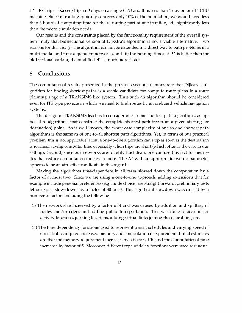
� � ��� ����� trips� � � � sec/trip ��� days on a single CPU and thus less than 1 day on our 14 CPU

machine. Since re-routing typically concerns only 10% of the population, we would need lessthan 3 hours of computing time for the re-routing part of one iteration, still significantly lessthan the micro-simulation needs.

Our results and the constraints placed by the functionality requirement of the overall sys-tem imply that bidirectional version of Dijkstra’s algorithm is not a viable alternative. Tworeasons for this are: (i) The algorithm can not be extended in a direct way to path problems in amulti-modal and time dependent networks, and (ii) the running times of � � is better than thebidirectional variant; the modified � � is much more faster.

8 Conclusions

The computational results presented in the previous sections demonstrate that Dijkstra’s al-gorithm for finding shortest paths is a viable candidate for compute route plans in a routeplanning stage of a TRANSIMS like system. Thus such an algorithm should be consideredeven for ITS type projects in which we need to find routes by an on-board vehicle navigationsystems.

The design of TRANSIMS lead us to consider one-to-one shortest path algorithms, as op-posed to algorithms that construct the complete shortest-path tree from a given starting (ordestination) point. As is well known, the worst-case complexity of one-to-one shortest pathalgorithms is the same as of one-to-all shortest path algorithms. Yet, in terms of our practicalproblem, this is not applicable. First, a one-to-one algorithm can stop as soon as the destinationis reached, saving computer time especially when trips are short (which often is the case in oursetting). Second, since our networks are roughly Euclidean, one can use this fact for heuris-tics that reduce computation time even more. The A � with an appropriate overdo parameterapperas to be an attractive candidate in this regard.

Making the algorithms time-dependent in all cases slowed down the computation by afactor of at most two. Since we are using a one-to-one approach, adding extensions that forexample include personal preferences (e.g. mode choice) are straightforward; preliminary testslet us expect slow-downs by a factor of 30 to 50. This significant slowdown was caused by anumber of factors including the following:

(i) The network size increased by a factor of 4 and was caused by addition and splitting ofnodes and/or edges and adding public transportation. This was done to account foractivity locations, parking locations, adding virtual links joining these locations, etc.

(ii) The time dependency functions used to represent transit schedules and varying speed ofstreet traffic, implied increased memory and computational requirement. Initial estimatesare that the memory requirement increases by a factor of 10 and the computational timeincreases by factor of 5. Moreover, different type of delay functions were used for induc-

15

ing a qualitatively different exploration of the network by the algorithm. This seems toprohibit keeping a small number of representative time dependency functions.

(iii) The algorithm for handling modal constraints works by making multiple copies of theoriginal network. The algorithm is discussed in [JBM98] and preliminary computationalresults are discussed in [Ko98]. This increased the memory requirement by a factor of 5and computation time by an additional factor of 5.

Extrapolations of the results for the Portland case study show that, even with this slowdownthe route planning part of TRANSIMS still uses significantly less computing time than themicro-simulation.

Finally, we note that under certain circumstances the one-to-one approach chosen in thispaper may also be useful for ITS applications. This would be the case when customers wouldrequire customized route suggestions, so that re-using a shortest path tree from another calcu-lation may no longer be possible.

Acknowledgments: Research supported by the Department of Energy under Contract W-7405-ENG-36. We thank the members of the TRANSIMS team in particular, Doug Anson, ChrisBarrett, Richard Beckman, Roger Frye, Terence Kelly, Marcus Rickert, Myron Stein and PatriceSimon for providing the software infrastructure, pointers to related literature and numerousdiscussions on topics related to the subject. The second author wishes to thank Myron Steinfor long discussion on related topics and for his earlier work that motivated this paper. Wealso thank Joseph Cheriyan, S.S. Ravi, Prabhakar Ragde, R. Ravi and Aravind Srinivasan forconstructive comments and pointers to related literature. Finally, we thank the referees forhelpful comments and suggestions.

16

References

[AMO93] R. K. Ahuja, T. L. Magnanti and J. B. Orlin, Network Flows: Theory, Algorithms andApplications, Prentice-Hall, Englewood Cliffs, NJ, 1993.

[AHU] A. V. Aho, J. E. Hopcroft and J. D. Ullman, The Design and Analysis of Computer Algo-rithms, Addison Wesley, Reading MA., 1974.

[BJM98] C. Barrett, R. Jacob, M. Marathe, Formal Language Constrained Path Problems to be pre-sented at the Scandinavian Workshop on Algorithmic Theory, (SWAT ’98), Stockholm,Sweden, July 1998. Technical Report, Los Alamos National Laboratory, LA-UR 98-1739.

[TR+95a] C. Barrett, K. Birkbigler, L. Smith, V. Loose, R. Beckman, J. Davis, D. Roberts and M.Williams, An Operational Description of TRANSIMS, Technical Report, LA-UR-95-2393,Los Alamos National Laboratory, 1995.

[CS97] R. Beckman et. al. TRANSIMS-Release 1.0 – The Dallas Fort Worth Case Study, LA-UR-97-4502

[CGR96] B. Cherkassky, A. Goldberg and T. Radzik, Shortest Path algorithms: Theory and Exper-imental Evaluation, Mathematical Programming, Vol. 73, 1996, pp. 129–174.

[GGK84] F. Glover, R. Glover and D. Klingman, Computational Study of am Improved ShortestPath Algorithm, Networks, Vol. 14, 1985, pp. 65–73.

[EL82] R. Elliott and M. Lesk, “Route Finding in Street Maps by Computers and People,”Proceedings of the AAAI-82 National Conference on Artificial Intelligence, Pittsburg, PA,August 1982, pp. 258-261.

[HNR68] P. Hart, N. Nilsson, and B. Raphel, “A Formal Basis for the Heuristic Determinationof Minimum Cost Paths,” IEEE Trans. on System Science and Cybernetics, (4), 2, July1968, pp. 100-107.

[HM95] Highway Research Board, Highway Capacity Manual, Special Report 209, National Re-search Council, Washington, D.C. 1994.

[JBM98] R. Jacob, C. Barrett and M. Marathe Models and Efficient Algorithms for Routing Problemsin Time Dependent and Labeled Networks, Technical Report, LA-UR-98-xxxx, Los AlamosNational Laboratory, 1998.

[Ko98] G. Konjevod, et al. Experimental Analysis of Routing Algorithms in in Time Dependent andLabeled Networks, in preparation, 1998.

[LR89] M. Luby and P Ragde, “A Bidirectional Shortest Path Algorithm with Good AverageCase Behavior,” Algorithmica, 1989, Vol. 4, pp. 551-567.

17

[Ha92] R. Hassin, “Approximation schemes for the restricted shortest path problem,” Mathe-matics of Operations Research, vol. 17, no. 1, pp. 36-42 (1992).

[Ma] Y. Ma, “A Shortest Path Algorithm with Expected Running time� � � � ����� �

,” Mas-ter’s Thesis, University of California, Berkeley.

[MCN91] J.F. Mondou, T.G. Crainic and S. Nguyen, Shortest Path Algorithms: A ComputationalStudy with C Programming Language, Computers and Operations Research, Vol. 18,1991, pp. 767–786.

[NB97] K. Nagel and C. Barrett, Using Microsimulation Feedback for trip Adaptation for RealisticTraffic in Dallas, International Journal of Modern Physics C, Vol. 8, No. 3, 1997, pp.505-525.

[NB98] K. Nagel, Experiences with Iterated Traffic Microsimulations in Dallas, in D.E. Wolf andM. Schreckenberg, eds. Traffic and Granular flow II Springer Verlag 1998. TechnicalReport, Los Alamos National Laboratory, LA-UR 97-4776.

[Pa74] U. Pape, Implementation and Efficiency of Moore Algorithm for the Shortest Root Problem,Mathematical Programming, Vol. 7, 1974, pp. 212–222.

[Pa84] S. Pallottino, Shortest Path Algorithms: Complexity, Interrelations and New Propositions,Networks, Vol. 14, 1984, pp. 257–267.

[Po71] I. Pohl, “Bidirectional Searching,” Machine Intelligence, No. 6, 1971, pp. 127-140.

[SV86] R. Sedgewick and J. Vitter “Shortest Paths in Euclidean Graphs,” Algorithmica, 1986,Vol. 1, No. 1, pp. 31-48.

[SI+97] T. Shibuya, T. Ikeda, H. Imai, S. Nishimura, H. Shimoura and K. Tenmoku, “FindingRealistic Detour by AI Search Techniques,” Transportation Research Board Meeting,Washington D.C. 1997.

[ZN98] F. B. Zhan and C. Noon, Shortest Path Algorithms: An Evaluation using Real Road Net-works Transportation Science, Vol. 32, No. 1, (1998), pp. 65–73.

18

Appendix: Description of Basic Algorithms

In this section, we describe the basic algorithms considered in this paper. Most of the resultsin this section are not new; we recall them here for completeness and for description of experi-mental results.

8.1 Dijkstra’s Algorithm

Dijkstra’s algorithm solves the single source shortest path problem on a weighted (un)directedgraph

���������, when all the edge weights are nonnegative. Let � � � ��� denote the weight of an

edge in the network.Suppose we wish to find a shortest path from

�to � . Dijkstra’s algorithm maintains a set�

of vertices whose final shortest paths from the source�

have been already computed. Thealgorithm repeatedly finds a vertex in the set � � �����

which has the minimum shortest pathestimate, adds � to

�and updates the shortest path estimates of all the neighbors of � that

are not in�

. The algorithm continues until the terminal vertex is added to�

. In general, itis convenient to think of the vertices in the graph being divided into three classes during theexecution of the algorithm: (i) shortest path tree vertices – (those which have been added to

�and

hence their shortest path has already been determined, (ii) unseen vertices – those for which thedistance estimate is � and (iii) fringe vertices – those that are adjacent to the vertices in

�but

have themselves not been added to�

. Now each iteration of the algorithm consists of adding afringe vertex with minimum distance to the shortest path tree and updating its neighbors to befringe vertices. Using this terminology, initially, only

�is a shortest path tree vertex, neighbors

of�

are fringe vertices, and others are unseen vertices.DIJKSTRA’S ALGORITHM outlines the steps of the algorithm. In the remainder of the section,

we will use � � � to denote the cost of a shortest path from�

to � . We will also assume that � �

�and

� �� . Also, for a given vertex

�let � � ��

denote the set of neighbors of�

i.e.� � �

��� � � � � � � ��� . Finally, by the phrase extract a vertex from�

we mean choose a vertexand delete it from

�.

8.2 Bidirectional Dijkstra’s Algorithm

The bidirectional algorithm has been used in the operations research community and ana-lyzed by theoretical computer scientists providing quantitative reasons for its improved per-formance. (See [LR89, Ma] for more details.) The bidirectional search algorithm consists oftwo phases. In the first phase we alternate between two unidirectional searches: one forwardfrom

�, growing a tree spanning a set of nodes

�for which the minimum distance from

�is

known, and the second that consists of growing a tree spanning a set of nodes � for which theminimum distance from

�is known. We alternately add one node to

�and one to � until an

edge crossing from�

to � is drawn. At this point, the shortest path is known to lie within thesearch trees associate with

�and � except for one additional edge from

�to � .

19

DIJKSTRA’S ALGORITHM:

� Input:���������

- a network, a source�

and a destination vertex�

and a non-negativeweight function

��� �������.

� 1. Initialization: Set�� ,

� ��� �

�and � � � � � � � ����� � � � � . Found = 0.

2. Iterative Step: while Found = 0 do

(a) Extract Minimum Step: Among all vertices� � � ���

extract a vertex�

withminimum value of

� � ��. Set

��� � � � � . If

���

then set Found = 1.(b) Decrease (Update) Key: For each edge

� � � � , such that � � � � � , set

� � � ������ � � � � ��� � � �� � � � � � � .� Output: A shortest path from

�to�, i.e. a path � ��� ��� � � � � ����� where

�����

and�����

and the weight � � � ����� �

�� � � � � �"! � ��� � is the minimum over all paths from�

to�

8.3 A Modification For Euclidean Graphs: # � -Algorithm

When the underlying network is Euclidean, it is possible to improve the average case perfor-mance of Dijkstra’s algorithm. Euclidean graphs are defined as follows. The vertices of thegraph correspond to points in $&% and the weight of each edge is proportional to the Euclideandistance between the two points. Typically, while solving problems on such graphs, the inher-ent geometric information is ignored by the classical path finding algorithms. The basic ideabehind improving the performance of Dijkstra’s algorithm is from Sedgewick and Vitter [SV86]and is originally attributed to Hart Nilsson and Raphel [HNR68] is simple and can be describedas follows. To build a shortest path from

�to � , we use the original distance estimate for the

fringe vertex such as � , i.e. from�

to � (as before) plus the Euclidean distance from � to � . Thuswe use global information about the graph to guide our search for shortest path from

�to � . To

formalize this, define � � ��('

to be the Euclidean distance between � and'

and define� �

��('

tobe the shortest path from � to

'in the graph. The length of the path as usual is equal to the sum

of the edge lengths that constitute the path: the weight of an edge�

��('

is defined to be � � ��('

.Now each fringe vertex � is assigned the following value: �����*) � � ��� � � +� � � � � �

�,� � � �� �

The resulting algorithm runs much faster than Dijkstra’s algorithm on typical graphs for thefollowing reasons: (i) The shortest path tree grows in the direction of � and (ii) The search of theshortest path can be terminated as soon as � is added to the to the shortest path tree. The cor-rectness of the algorithm follows from the fact that � � �

� � is a lower bound on� �

�� � . Another

way to interpret the algorithm and its correctness is by using the concept of vertex potentials –an idea first used by Gabow.Concept of Vertex Potentials. Each vertex is assigned a non-negative value � � �

– called its

potential. The intuition is, that we put the vertices in a mountainous region – i.e. we assign aaltitude to them. Furthermore we take the edge-weights as the energy needed to get from oneend of the edge to the other. Then the resulting energy (cost) needed to traverse an edge is theoriginal cost modified by the potential (energy) difference of the endpoints. This leads to the

20

following formal definition:

� � � ��� � ��� �� � � ���� � � � � ��� &� � � � � � � ��

The potentials are called admissible or feasible if the new lengths are all positive. The follow-ing theorem shows that the the shortest paths in the graph with modified weights remains thesame.

Theorem 8.1 Let � be a set of admissible vertex potential. Then the weight of a path � ��� ��� � � � � � � � � � � from

�to � is given by

�� � � �� ����� �

� � � � � � � � &� � ��� � � � �

In other words the length of each path from�

to � is changed by the same constant additive amount.Thus if � is a shortest

� � � path in the original graph then it is still the shortest path in the graph withmodified edge weights.

8.4 Modified # �We briefly discuss some of the heuristic improvements to the basic � � algorithm that can beused in practice. Again, recall that in many practical situations (including TRANSIMS), it isnot necessary to find exact shortest paths – approximately shortest paths suffice. We tried twoheuristic solutions in this context.(1) The modified � � algorithm. Recall that the ��� algorithm (implicitly) takes the estimate(here the Euclidean distance) as an potential. As long as this estimate is a lower bound on theshortest paths for all pairs of nodes, the graph modified by the potential still has only non-negative weights and Dijkstra’s algorithm works correctly. If we now increase the influenceof the potential by multiplying it, this correctness doesn’t have to be maintained. Neverthe-less we get an fast heuristic algorithm that produces simple path, that turn out to be still ofinterestingly high quality. An important advantage of this method is, that we can choose this“overdo parameter”, which reflects the strength of the potential all the way from 1 (correct) to� in which case the algorithm always expands the node next (Euclidean) to destination, whichtends to be very fast. Note that the usefulness of this heuristic heavily depends on the graph itis used on. As our results in Section 6 point out, it appears that an appropriate constant resultsin a very good trade-off between quality of solution and the time required.(2) Combining � � with Bidirectional Search The discussion in the above sections suggestscombining the bidirectional search heuristic with the � � search. One possible way to do itis to use two potentials ��� � � and ��� � � for each vertex, the potentials reflecting the lowerbounds (usually geometric distances) of � from

�and � . A naive implementation of this idea is

unfortunately incorrect, since the two potentials imply building shortest path trees from�

and� . As shown in [SI+97], a modified potential suffices to ensure the correctness of the algorithm.

21

9 Discussion on Data Structures

(1) Arrays versus Heaps. In a naive implementation of the algorithm using an array�

, inwhich for each vertex,

� � we store the value of� � � � in location

� ��� . In each iteration Extract

Minimum Key takes��� �

time (finding a minimum value in an unsorted array takes��� �

time)and Decrease Key takes time

� � � ��� � �� . Here� ��� � � denotes the degree of

�. The total running

time is therefore��� ��� � � � ��� � � � � � �� � . Using Binary Heaps (as has been done in the

current implementation of the algorithm), we can improve the running time. First considerExtract Minimum Key operation. The time to do this is

� � � ��� � since we simply pick the top of

the heap and then process the data structure to maintain the heap property (using HEAPIFY).Next consider the Decrease Key operation. This operation takes time

� � � ��� � � ����� � for thefollowing reason. We need to update the distance estimate for each of the

� ��� � � neighbors,each operation taking time

� � � ��� � . The time to build the heap for the first time is

� � � .

Thus the total running time of the algorithm is�� � � � � ��� � � � ��� � � ����� � �

� � � � ��� � � ����� �

���� � � ����� � . We also considered using Fibonacci Heaps. Our experimental

analysis revealed that typically the number of nodes that are kept in a heap is around 500; thususing a more sophisticated data structure with higher constants was not likely to yield betterresults in practice. Using Fibonacci heaps could potentially improve the theoretical runningtime of the algorithm by of

����� ��� , where

�denotes the maximum heap size at any stage of

the execution. This implies an improvement of at most a factor of � . But the constants with theheap operations and the complicated code for implementing this data structure weigh moreheavily against it.

(2) Deferred Update. Recall that we need to update the values of the distance estimates in Step2b of DIJKSTRA’S ALGORITHM. Assume that the heap is

�, and degree of a node

�being

� �, it

would take roughly � � � ����� � operations to update the distance estimates. The reason for thisis as follows: We can maintain an auxiliary array that keeps pointers to the nodes in the heap.Every time a nodes distance estimate is updated, the node moves through the heap (as a partof HEAPIFY operation) to settle in the final position. During the course of this other nodeson its path also change positions. This implies that the pointed values for each of the nodesneed be updated. (We are assuming an array implementation of the Heap.) Another possibleway to do this is to insert multiple copies of a node in the heap. In this way, the time taken isroughly proportional to adding these nodes plus the additional factor depending on the sizeof the heap for future operations. Again, let

� �denote the degree of a node and

�� ����be the

maximum degree. Then the heap size grows at most by a multiplicative factor of�� ����

. Sincethe Heap operations take time roughly

����� �this implies that the total time for executing Step

2b is no more than� ���� ����� � � ���� �

which is� ���� � � ��� � � ����� � ����

. Typically, the averagedegree of a node in the Case study network is � ������� and you expect that it only gets insertedroughly only by half its neighbors resulting in an average increase of no more than � on thesize of the heap. This implies that we spend only an additional additive factor of � � � for eachrun of Step 2b.

(3) Hash Tables for Storing Graphs. The graph we received from Dallas MPO is given using

22

long Link and Node Id’s. Although the naming convention is useful in other contexts, such anaming convention yields a inefficient use of the domain space. To illustrate the point, the linkand the node It’s given were typically made of 32 bits long. Thus the name space of for thenodes is roughly � � � . In contrast the number of nodes is roughly

����� � � � �. Such a discrepancy

immediately motivated a use of hash tables to improve the name space utilization. We used aHash table of size roughly � � �

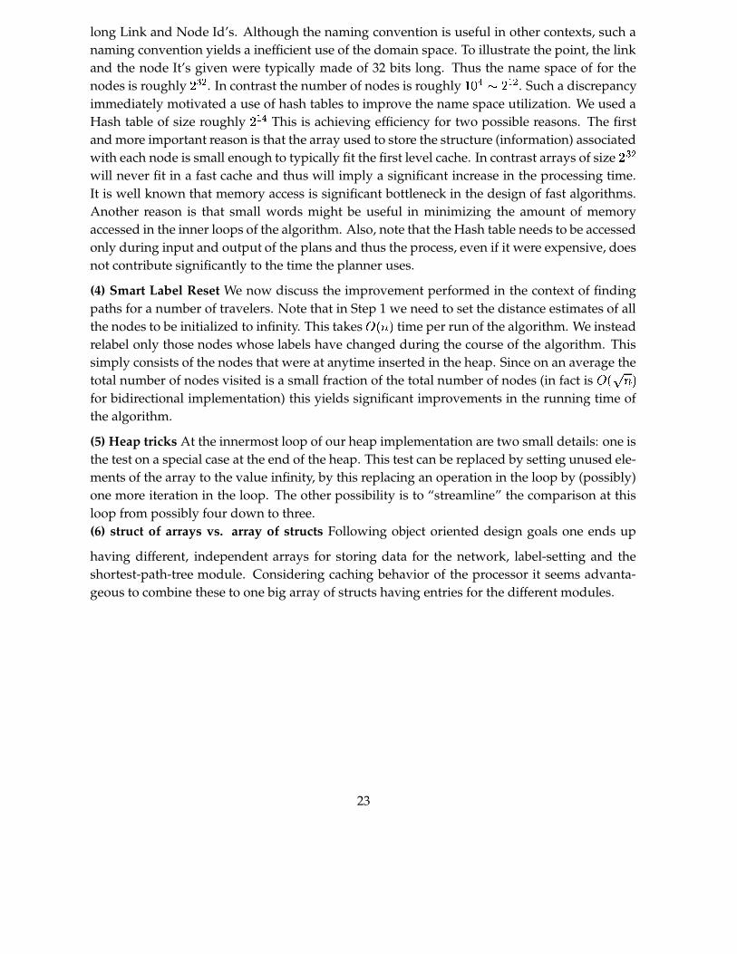
This is achieving efficiency for two possible reasons. The firstand more important reason is that the array used to store the structure (information) associatedwith each node is small enough to typically fit the first level cache. In contrast arrays of size � � �will never fit in a fast cache and thus will imply a significant increase in the processing time.It is well known that memory access is significant bottleneck in the design of fast algorithms.Another reason is that small words might be useful in minimizing the amount of memoryaccessed in the inner loops of the algorithm. Also, note that the Hash table needs to be accessedonly during input and output of the plans and thus the process, even if it were expensive, doesnot contribute significantly to the time the planner uses.

(4) Smart Label Reset We now discuss the improvement performed in the context of findingpaths for a number of travelers. Note that in Step 1 we need to set the distance estimates of allthe nodes to be initialized to infinity. This takes

��� � time per run of the algorithm. We instead

relabel only those nodes whose labels have changed during the course of the algorithm. Thissimply consists of the nodes that were at anytime inserted in the heap. Since on an average thetotal number of nodes visited is a small fraction of the total number of nodes (in fact is

� � � � for bidirectional implementation) this yields significant improvements in the running time ofthe algorithm.

(5) Heap tricks At the innermost loop of our heap implementation are two small details: one isthe test on a special case at the end of the heap. This test can be replaced by setting unused ele-ments of the array to the value infinity, by this replacing an operation in the loop by (possibly)one more iteration in the loop. The other possibility is to “streamline” the comparison at thisloop from possibly four down to three.(6) struct of arrays vs. array of structs Following object oriented design goals one ends up

having different, independent arrays for storing data for the network, label-setting and theshortest-path-tree module. Considering caching behavior of the processor it seems advanta-geous to combine these to one big array of structs having entries for the different modules.

23