a computational model of red blood cell dynamics in patients with

A Computational Model of Red Blood Cell Dynamics in Patients

with Chronic Kidney Disease

H. T. Banks1, Karen M. Bliss1, Peter Kotanko2, Hien Tran1

1Center for Research in Scientific Computation, North Carolina State University2Renal Research Institute, New York

February 15, 2011

Abstract

Kidneys are the main site of production of the hormone erythropoietin (EPO) that is themajor regulator of erythropoiesis, or red blood cell production. EPO level is normally controlledby a negative feedback mechanism in the kidneys, but patients with chronic kidney disease (CKD)do not produce sufficient levels of EPO to maintain appropriate blood hemoglobin concentration.A mathematical model, including interactions with iron and inflammation, is developed for ery-thropoiesis in patients with CKD. Numerical solution methodologies and validation of numericalresults are discussed. Simulation results under varying conditions and treatment protocols arepresented.

Further author information: (Send correspondence to Karen M. Bliss.)

Karen M. Bliss: [email protected]. T. Banks: [email protected] Kotanko: [email protected] Tran: [email protected]

1

1 Introduction

It is estimated that 31 million Americans have chronic kidney disease (CKD). Among those, approx-imately 330 thousand are classified as being in End-Stage Renal Disease (ESRD) and require dialysis[17]. Dialysis is the bidirectional exchange of materials across a semipermeable membrane [2]. Forthe purposes of this study, we consider only hemodialysis, where a patient’s blood is exposed to asemipermeable membrane outside of the body.

In addition to regulating blood pressure and filtering waste products from blood, kidneys producea hormone called erythropoietin (EPO) that is the major regulator of erythropoiesis, or red blood cellproduction. EPO level is normally controlled by a negative feedback mechanism in the kidneys, butpatients in ESRD do not produce sufficient levels of EPO to maintain blood hemoglobin concentra-tion. Hemoglobin is the protein that gives red blood cells the ability to carry oxygen. Patients withlow hemoglobin concentration may present symptoms of anemia, such as decreased cardiac function,fatigue, and decreased cognitive function.

In order to prevent anemia, patients typically receive recombinant human EPO (rHuEPO) in-travenously to stimulate red blood cell production. However, treatment is far from perfect. In 2006,only half of dialysis patients had a mean monthly hemoglobin greater than 11 grams per deciliter[17], the desired minimum level set by the National Kidney Foundation [13].

Iron is required to produce hemoglobin, and iron deficiency can be an issue among patientsreceiving rHuEPO therapy. Oral iron supplementation is often ineffective, so intravenous iron sup-plementation has become a mainstay in many patients undergoing rHuEPO therapy [9].

Iron availability is negatively affected by inflammation level in the body. Most patients withCKD have elevated levels of inflammation due to CKD and the presence of other medical issues (e.g.,diabetes, hypertension, etc.) [10].

Our goals are (1) the development of a mathematical model for erythropoiesis of patients in ESRDundergoing hemodialysis, taking into consideration the effects of EPO, iron level, and inflammationlevel in the body, which has a reasonable degree of fidelity to the biological system, and (2) thedevelopment of model-based control of the system. This note is a step toward the first of these twogoals.

2 Erythropoiesis

Erythropoiesis is the process by which erythrocytes, or red blood cells (RBCs), are formed. Erythro-cytes transport oxygen and carbon dioxide between the lungs and all of the tissues of the body andcan be thought of as a container for hemoglobin [15], the protein that carries oxygen.

Erythrocytes are produced primarily from pluripotent stem cells in bone marrow. In the presenceof the cytokine named stem cell factor, hematopoietic stem cells divide asymetrically, producing acommitted colony-forming-unit (CFU) while maintaining the population of stem cells. The erythro-cyte lineage shares the precursor CFU-GEMM (granulocyte, erythrocyte, macrophage, megakary-ocyte) with other types of blood cells (white blood cells, platelets, etc.). The exact mechanismsdetermining selection of lineage from this nodal point are not known [6].

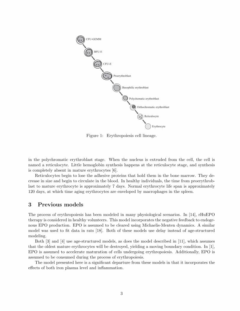
Erythrocyte lineage continues as described in Figure 1: erythroid burst-forming unit (BFU-E), erythroid colony-forming-unit (CFU-E), proerythrocyte, basophilic erythrocyte, polychromaticerythroblast, orthochromatic erythroblast, reticulocyte, and erythrocyte. Cell division ceases withthe formation of the orthochromatic erythroblast. Division rate, death rate, and maturation rate areinfluenced by the level of EPO [6]. This is described in more detail later.

Hemoglobin is synthesized beginning in the CFU-E stage, with the majority of synthesis occurring

2

CFU-GEMMC

BFU-E

CFU-E

Proerythroblast

Basophilic erythroblast

Polychomatic erythroblast

Orthochromatic erythroblast

Reticulocyte

Erythrocyte

Figure 1: Erythropoiesis cell lineage.

in the polychromatic erythroblast stage. When the nucleus is extruded from the cell, the cell isnamed a reticulocyte. Little hemoglobin synthesis happens at the reticulocyte stage, and synthesisis completely absent in mature erythrocytes [6].

Reticulocytes begin to lose the adhesive proteins that hold them in the bone marrow. They de-crease in size and begin to circulate in the blood. In healthy individuals, the time from proerythrob-last to mature erythrocyte is approximately 7 days. Normal erythrocyte life span is approximately120 days, at which time aging erythrocytes are enveloped by macrophages in the spleen.

3 Previous models

The process of erythropoiesis has been modeled in many physiological scenarios. In [14], rHuEPOtherapy is considered in healthy volunteers. This model incorporates the negative feedback to endoge-nous EPO production. EPO is assumed to be cleared using Michaelis-Menten dynamics. A similarmodel was used to fit data in rats [18]. Both of these models use delay instead of age-structuredmodeling.

Both [3] and [4] use age-structured models, as does the model described in [11], which assumesthat the oldest mature erythrocytes will be destroyed, yielding a moving boundary condition. In [1],EPO is assumed to accelerate maturation of cells undergoing erythropoiesis. Additionally, EPO isassumed to be consumed during the process of erythropoiesis.

The model presented here is a significant departure from these models in that it incorporates theeffects of both iron plasma level and inflammation.

3

4 Model Overview

We use an age-structured model with three major classifications of erythroid cells in which thestructure variables µ, ν, and ψ represent maturity levels, as shown in Figure 2.

EPO

Inflammation

Iron

RBC Progenitors, P(t, µ)

Maturing RBCs, M(t, ν)

Oxygen-carrying capacity, O(t, ψ)

hemoglobin in RBCs

recr

uitm

ent r

ate

birth

rate

and

dea

th ra

te

mat

urat

ion

rate

deat

h ra

te

EPO clearance

EPO produced in the liver and kidney

intravenous EPO

treatment

iron losses

intravenous iron treatment

Figure 2: Model schematic.

P (t, µ) and M(t, ν) represent the number of progenitor cells and maturing hematopoietic cells,respectively. O(t, ψ) is a measure of the oxygen carrying capacity of circulating reticulocytes anderythrocytes. For these cell classes, the second argument (e.g., µ for class P ) is the structurevariable, maturity level in this case. We model EPO level, E, iron level, Fe, and a measure of overallinflammation in the body, I. Time is measured in days.

Our state variables are

P = P (t, µ), M = M(t, ν), O = O(t, ψ), E = E(t), and Fe = Fe(t).

Rate of exogenous EPO treatments, Eex, and rate of exogenous iron treatments, Feex, are inputfunctions, and hemoglobin concentration, Hb(t), is the output of the model.

We will make use of sigmoid functions throughout the model. An increasing sigmoid functionwill be of the form

F (x) =(Fmin − Fmax

)· ck

ck + xk+ Fmax.

Note that when x is small, F (x) is close to Fmin, and when x is large, F (x) is close to Fmax. Thetypical graph of such a function is depicted in Figure 3a. The values of c and k affect the slope ofthe curve and the location of the area of increase.

Similarly, a typical decreasing sigmoid function is depicted in Figure 3b and has the form

G(x) =(Gmax −Gmin

)· ck

ck + xk+Gmin.

4

F(x)

Fmax

Fmin

x

(a) Generic increasing sigmoid function.

G(x)

Gmax

Gmin

x

(b) Generic decreasing sigmoid function.

Figure 3: Sigmoid function examples.

5 Iron

Iron is required to make hemoglobin, the protein that gives erythrocytes the ability to carry oxygen.It is also the protein that gives erythrocytes their characteristic red color. If iron is not availableduring erythropoiesis, the result is lighter-colored (hypochromic) erythrocytes with reduced capacityto carry oxygen.

Control of iron in the body is a strictly regulated process, in part because there is no pathwayfor the excretion of excess iron (Figure 4).

Blood Plasma (iron is carried in transferrin)

Spleen (removes old RBCs

and recycles iron from the

hemoglobin)

Bone Marrow (RBCs produced,

which contain iron in their hemoglobin)

~20 mg iron/day

~20 mg iron/day

RB

Cs c

ircul

atin

g in

blo

od

Liver (stores iron)

Iron losses

Iron from diet

~2 mg iron/day

~2 mg iron/day

Figure 4: Iron cycle in healthy individuals.

5

When red blood cells age, they become enveloped by macrophages in the spleen. The iron fromtheir hemoglobin is then recaptured and sent to the bone marrow for use in making hemoglobinfor new erythrocytes. This recycling process is very efficient and is the main source of iron toerythropoiesis [15]. In much smaller quantities, iron is absorbed from diet in the duodenum and canbe stored in the liver. The only losses to the system are from sweating, cells being shed, blood losses,etc.

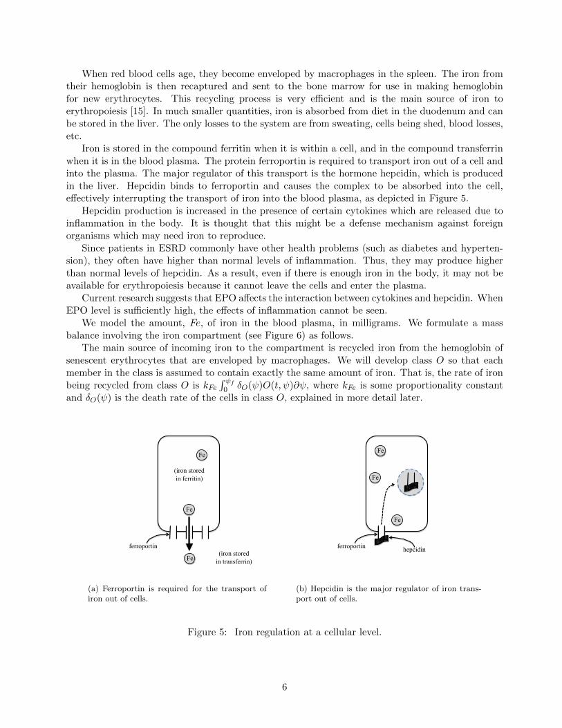
Iron is stored in the compound ferritin when it is within a cell, and in the compound transferrinwhen it is in the blood plasma. The protein ferroportin is required to transport iron out of a cell andinto the plasma. The major regulator of this transport is the hormone hepcidin, which is producedin the liver. Hepcidin binds to ferroportin and causes the complex to be absorbed into the cell,effectively interrupting the transport of iron into the blood plasma, as depicted in Figure 5.

Hepcidin production is increased in the presence of certain cytokines which are released due toinflammation in the body. It is thought that this might be a defense mechanism against foreignorganisms which may need iron to reproduce.

Since patients in ESRD commonly have other health problems (such as diabetes and hyperten-sion), they often have higher than normal levels of inflammation. Thus, they may produce higherthan normal levels of hepcidin. As a result, even if there is enough iron in the body, it may not beavailable for erythropoiesis because it cannot leave the cells and enter the plasma.

Current research suggests that EPO affects the interaction between cytokines and hepcidin. WhenEPO level is sufficiently high, the effects of inflammation cannot be seen.

We model the amount, Fe, of iron in the blood plasma, in milligrams. We formulate a massbalance involving the iron compartment (see Figure 6) as follows.

The main source of incoming iron to the compartment is recycled iron from the hemoglobin ofsenescent erythrocytes that are enveloped by macrophages. We will develop class O so that eachmember in the class is assumed to contain exactly the same amount of iron. That is, the rate of ironbeing recycled from class O is kFe

∫ ψf

0 δO(ψ)O(t, ψ)∂ψ, where kFe is some proportionality constantand δO(ψ) is the death rate of the cells in class O, explained in more detail later.

(iron stored in ferritin)

(iron stored in transferrin)

ferroportin

Fe

Fe

Fe

(a) Ferroportin is required for the transport ofiron out of cells.

ferroportin hepcidin

Fe

Fe

Fe

(b) Hepcidin is the major regulator of iron trans-port out of cells.

Figure 5: Iron regulation at a cellular level.

6

EPO

Inflammation Iron

Oxygen-carrying capacity, O(t, ψ)

iron losses

intravenous iron treatment

Maturing RBCs, M(t, ν)

Figure 6: Iron compartment.

The other main source of iron to the compartment is exogenous iron supplied as part of treatment.We denote the rate of exogenous iron treatment by Feex(t)

A small amount of iron enters the system through absorption from diet and from storage inthe liver, and there are also iron losses (due to sweating, blood losses during blood draws andhemodialysis, etc.). As described earlier, patients undergoing hemodialysis require iron supplementsintravenously. Therefore we assume that when we sum the iron losses and the iron entering thesystem from diet and storage in the liver we obtain a net loss. Further, we will assume for an initialmodel that the loss occurs at constant rate unless the current level of iron is small, in which case afraction of the iron is lost. That is, that rate of iron loss, ρFe,loss(Fe), is given by

ρFe,loss(Fe) =

{ρFe,const, Fe ≥ FethρFe,frac · Fe, Fe < Feth.

This assumption will be revisited in future models, perhaps with greater losses when dialysis andblood draws occur.

Next we need to account for iron leaving the compartment during erythropoiesis. For our firstmodel, we begin by making the assumption that iron enters red blood cells at the moment that a cellmatures from class M to class O, which is the time that a cell leaves the bone marrow and beginscirculating. Red blood cells actually collect iron over the time period that they are in class M, butthe biochemistry of this process is not clearly understood. The assumption that all of the iron iscollected into a cell at one moment will certainly have to be revisited in future improvements of themodel.

In determining the amount of iron used during erythropoiesis, we first compute the amount ofiron that would be used if every cell leaving class M were to contain the appropriate amount ofhemoglobin so as to be at full oxygen-carrying capacity, i.e.,

Feneeded = kFeM(t, νf ). (1)

In the presence of inflammation, even if there is enough iron in the plasma, it may not be availableto be used in erythropoiesis. For our initial model, we assume that there is an EPO threshold, EPOth.

7

We assume that if EPO is above the threshold, the effects of inflammation can not be seen. That is,we assume

Feavail = kFe,efff(E, I)Fe, (2)

where

f(E, I) =

(cFe,av)

kFe,av

(cFe,av)kFe,av+ IkFe,av

, E < EPOth

1, E ≥ EPOth.

Observe that in this model when EPO is greater than the threshold level, inflammation leveldoes not impact iron availability. However, when EPO level is lower than the threshold, the amountof available iron depends on inflammation level–as f(E, I) is close to one when inflammation is lowand close to zero when inflammation is high. The constant kFe,eff , with 0 ≤ kFe,eff ≤ 1, is an efficacyconstant that accounts for the fact that only a fraction of the iron in the plasma will actually beavailable at the site of erythropoiesis at any given time.

The amount of iron actually used in erythropoiesis is therefore given by

Feused = min {Feneeded, Feavail} ,= min {kFeM(t, νf ), kFe,efff(E, I)Fe} . (3)

We assume that the rate of iron leaving the iron compartment and entering class O is proportionalto this quantity, Feused. That is,

ρFe→O = kρ,FeFeused.

Thus, the mass balance in the iron compartment is given by

Fe(t) = (rate in from class O) + (rate in intravenously)

− (rate out to class O)− (rate of iron losses)

= kFe

∫ ψf

0δO(ψ)O(t, ψ)dψ + Feex(t)− ρFe→O − ρFe,loss(Fe). (4)

6 EPO

EPO is the primary regulator of erythropoiesis. It stimulates red blood cell production, differentiationand maturation, and prevents apoptosis [6]. In healthy individuals, the majority of EPO productionoccurs in the kidney. Sensors in the kidney monitor blood oxygen level. EPO production is increasedin response to low oxygen level and is decreased when oxygen level is high.

Patients in ESRD, whose kidneys have only minimal function, produce only a small basal level ofEPO in the kidney and liver [7]. Without intervention, patients can develop anemia; therefore, pa-tients undergoing dialysis are commonly treated with intravenous rHuEPO. Two common rHuEPOs,epoetin alfa and epoetin beta, share structural homology with endogenous EPO. Darbepoietin alfa,the other major erythropoietic agent, is designed so that it has a longer half-life in-vivo. In thismodel, we assume that darbepoietin is not the erythropoietic agent, and therefore we will not dis-tinguish between rHuEPO and endogenous EPO with respect to their action. We assume that theireffects on erythropoiesis are identical.

8

EPO is measured in units of EPO. We assume the rate of endogenous EPO production in theliver and kidney to be constant, and will denote it ρEPO,basal.

We will assume that EPO clearance is proportional to the amount present, although we couldconsider Michaelis-Menten dynamics in future models. Finally, we also account for the rate of EPOgiven via IV, denoted Eex(t). So we have

E(t) = ρEPO,basal + Eex(t)− 1

t1/2ln 2·E(t),

where t1/2 is the half-life of EPO.

7 Inflammation

Inflammation affects two aspects of erythropoiesis, as depicted in Figure 2.Even in patients without CKD, chronic inflammation can cause anemia, termed the anemia of

chronic disease. While the exact chemical pathways are not necessarily known, it is known that thepresence of inflammation can suppress erythropoiesis and may inhibit the action of EPO [16]. SinceEPO affects the birth and death rate of progenitors, we incorporate inflammation in the death rateterm associated with the progenitor cell class, P.

Inflammation level also impacts iron availability for erythropoiesis, as described previously. In-flammation may cause an increase in ferritin production, which would cause iron to be retained withincells, inhibiting the use of iron to make hemoglobin. Inflammation may also impair the ability of thebody to absorb dietary iron [16].

It is almost certain that inflammation affects these two aspects of erythropoiesis via completelydifferent chemical pathways. We assume that both aspects can be sufficiently described with someoverall measure of inflammation in the body. There are markers of inflammation, such as albuminand C-reactive protein, which are often measured in patients undergoing dialysis. In future work, wewill investigate whether inflammation can be described as some combination of the levels of thesemarkers.

8 Class P (t, µ)

We group the progenitor cells (CFU-GEMM, BFU-E and CFU-E) in one class, P (t, µ). These cellsare affected by EPO level and inflammation level.

We make the following assumptions:

(i) There is a smallest maturity level, µ0 = 0, and a largest maturity level, µf ; i.e., 0 ≤ µ ≤ µf .

(ii) The maturity rate depends on the EPO concentration and the maturity level [6]. For simplifi-cation in our initial model, we assume that the maturity rate is constant:

dµ

dt= ρP .

(iii) The birth rate depends on EPO concentration [6] and the maturity level.

Regulation of erythropoiesis by EPO is focused on the progenitor class, and probably mostimportantly the CFU-E. A rise in EPO level results in proliferation of CFU-E [6]. We will

9

EPO

Inflammation

RBC Progenitors, P(t, µ)

to class M re

crui

tmen

t rat

e

birth

rate

and

dea

th ra

te

deat

h ra

te

Figure 7: The progenitor cells, P (t, µ).

assume EPO affects all cells in class P equally, independent of maturity level. We will modelthe birth rate as an increasing sigmoid function,

βP (E) =(βminP − βmaxP

) (cβ,P )kβ,P

(cβ,P )kβ,P + Ekβ,P+ βmaxP .

(iv) The number of stem cells being recruited into the precursor cell population is directly propor-tional to EPO level:

P (t, 0) = RPE(t).

It is reasonable to assume that recruitment is related to EPO level, as it is one of the hormonesthat affects whether a stem cell will become an erythrocyte. Other hormones are certainlyinvolved as well, but the chemical pathway governing the differentiation of stem cells is stilllargely unknown [6].

(v) The death rate depends on the concentration of EPO, the inflammation level, and the maturitylevel, µ. We will simplify this for our first model to assume that death rate is not dependenton maturity level.

EPO prevents apoptosis, or programmed cell death, of progenitor cells [6]. We use a decreasingsigmoid function to describe this behavior.

Certain interferons, present under inflammatory conditions, can also cause death of progenitorcells, specifically CFU-E [12]. We assume that the death rate of progenitor cells depends oninflammation level, which is modeled by some increasing sigmoid function.

Finally, we assume that overall death rate is the sum of these two effects:

δP (E, I) =(δmaxP,E − δminP,E

) (cδ,P,E)kδ,P,E

(cδ,P,E)kδ,P,E + Ekδ,P,E+ δminP,E

+(δminP,I − δmaxP,I

) (cδ,P,I)kδ,P,I

(cδ,P,I)kδ,P,I + Ikδ,P,I

+ δmaxP,I .

10

Now we consider the rate of change in population from maturity level µ to maturity level µ+ ∆µ.

rate of change in population on the interval (µ, µ+ ∆µ) =

(rate of cells entering the interval)− (rate of cells leaving the interval)

+ (birth rate term)− (death rate term)

∂

∂t

∫ µ+∆µ

µP (t, ξ)dξ = ρPP (t, µ)− ρPP (t, µ+ ∆µ)

+

∫ µ+∆µ

µβP (E)P (t, ξ)dξ −

∫ µ+∆µ

µδP (E, I)P (t, ξ)dξ

∂

∂t

∫ µ+∆µ

µP (t, ξ)dξ = − ρP [P (t, µ+ ∆µ)− P (t, µ)]

+ [βP (E)− δP (E, I)]

∫ µ+∆µ

µP (t, ξ)dξ

Dividing by ∆µ and then letting ∆µ→ 0, we obtain

∂

∂tP (t, µ) = −ρP

∂

∂µP (t, µ) + [βP (E)− δP (E, I)]P (t, µ),

and we have the boundary condition

P (t, 0) = RPE(t).

9 Class M(t, ν)

Class M(t, ν) consists of immature hematopoietic cells: proerythroblasts, basophilic erythroblasts,polychromatic erythroblasts, orthochromatic erythroblasts, and non-circulating reticulocytes (i.e.those that still reside in the bone marrow). Cells are recruited from class P and, upon maturation,feed into class O. Their development is influenced by EPO concentration.

We make the following assumptions:

(i) There is a smallest maturity level, ν0 = 0, and a largest maturity level, νf . That is, 0 ≤ ν ≤ νf .

(ii) The maturation rate depends on the level of erythropoietin and the maturity level. However,for our initial model, we assume that maturation rate does not depend on the maturity level.

EPO stimulates maturation [6], so we use an increasing sigmoid function for maturation rate,ρM (E) .

ρM (E) =(ρminM − ρmaxM

) (cρ,M )kρ,M

(cρ,M )kρ,M + Ekρ,M+ ρmaxM .

11

EPO

from class P Maturing RBCs, M(t, ν)

to class O

mat

urat

ion

rate

Figure 8: Maturing erythrocytes, M(t, ν).

(iii) The birth rate depends on the maturity level, but for our first model, we assume birth rate isa constant, βM .

(iv) The number of cells at maturity level ν = 0 is equal to the number of cells leaving the previousstage:

M(t, 0) = P (t, µF ).

(v) The death rate depends on the maturity level, ν and on the iron level. To simplify, we assumethe death rate is a constant, δM .

As in the progenitor class, we can consider the rate of change in population from maturity level ν tomaturity level ν + ∆ν, then divide by ∆ν and let ∆ν → 0 to obtain

d

dtM(t, ν) = −ρM (E)

∂

∂νM(t, ν) +

[βM − δM

]M(t, ν).

Since we have made the assumption that the birth and death rates are both constant, it is clearthat they will not both be identifiable. We replace the difference βM−δM by the constant βM , whichthen represents the net birth rate.

Hence, we have∂

∂tM(t, ν) = −ρM (E)

∂

∂νM(t, ν) + βMM(t, ν),

with the boundary conditionM(t, 0) = P (t, µF ).

It is worth noting again that as this is our first model of the system, we have made the assumptionthat iron level does not impact cell development until cells mature out of class M into class O.Specifically, we do not account for iron entering red blood cells throughout class M and we ignoreany impact this would have on death rate in class M. Future versions of the model will need toaccount for these interactions with the iron compartment.

12

10 Class O

Unlike the classes P and M, class O does not represent the number of circulating reticulocytesand mature erythrocytes, because knowledge of the number of cells alone does not give us enoughinformation to determine whether the cells contain the necessary amount of hemoglobin to carryoxygen at full capacity.

Erythrocytes begin hemoglobinization at the polychromatic erythroblast stage (in class M).They continue to acquire more hemoglobin throughout the orthochromatic erythroblast stage andinto the reticulocyte stage, until the reticulocyte leaves the bone marrow, at which time it ceaseshemoglobinization [15]. Hence, the oxygen carrying ability of a mature erythrocyte is determined byhow much hemoglobin is available during the time interval when that cell is in class M.

In order to initially simplify computations, we assume that a cell’s oxygen-carrying ability isbased solely on the availability of iron at the time that the cell matures out of class M and beginscirculating in the blood. As previously noted, the biology does not support this formulation of theproblem, and this assumption will be reconsidered in future models.

Let us consider an example in order to elucidate this idea. Suppose we know that kFe = 0.2mg/billion cells and that at some given time t, Feavail = 8 mg. Suppose also that at time t there are100 billion cells maturing out of class M ; that is, M(t, νf ) = 100. Then

Feavail < Feneeded = kFeM(t, νf ) = 20 mg.

Then, per equation (3), Feused = Feavail = 8 mg, which is only 40% of the 20 mg that would beneeded for each cell maturing into class O to have full oxygen-carrying capacity. Then the 100 billioncells maturing into class O would have, on average, only 40% oxygen-carrying ability. It would bedifficult to track both the number of circulating erythroid cells and the oxygen carrying capacity ofeach. Instead, we think of the 100 billion cells with 40% oxygen-carrying ability as 40 billion cellswith 100% oxygen-carrying capacity. Hence, every “cell” in class O is assumed to have full-oxygencarrying capacity.

Now we present the assumptions we make about class O.

(i) We assume that there is a smallest maturity level, ψ0 = 0, and a largest maturity level, ψf .That is, 0 ≤ ψ ≤ ψf . In the future, we may wish to allow ψf to vary.

(ii) The maturation rate of cells in this class is a function of the maturity level. We will furtherassume, for simplification in this initial model, that the maturity rate is constant:

dψ

dt= ρO

(iii) The birth rate is zero. Cells at this stage mature but do not proliferate [6].

(iv) The number of members of class O at maturity level ψ = 0 is equal to the number of cellsleaving the previous stage multiplied by the ratio of Feused and Feneeded:

O(t, 0) =FeusedFeneeded

·M(t, νf ),

=Feused

kFeM(t, νf )·M(t, νf ),

=1

kFeFeused. (5)

As stated above, this assumption guarantees that each member of class O has full oxygen-carrying ability.

13

(v) The death rate of cells in the class O(t, ψ), depends on the maturity level. We expect this tobe an increasing function, because macrophages envelop mainly aging adult erythrocytes [15].Therefore, we will use the increasing sigmoid function

δO(ψ) =(δminO − δmaxO

) (cδ,O)kδ,O

(cδ,O)kδ,O + ψkδ,O+ δmaxO .

As in classes P and M, we can generate the partial differential equation

∂

∂tO(t, ψ) = −ρO

∂

∂ψO(t, ψ)− δO(ψ)O(t, ψ)

with boundary condition (5).

11 Hemoglobin Concentration

We have already assumed that hemoglobin exists only in erythrocytes in class O. We compute thetotal number of members in class O at a given time t by∫ ψf

0O(t, ψ)dψ. (6)

We previously made the assumption that each member of class O has exactly the same amountof iron. Specifically, if we multiply the quantity (6) by kFe, we have the amount of iron (in mg)circulating in erythrocytes at time t. We then multiply by a conversion factor to find the amountof hemoglobin circulating. Then we need only divide by blood volume, BV (t), to determine thehemoglobin concentration.

Blood volume is difficult to determine and varies greatly in patients undergoing dialysis. Patientsin ESRD are unable to clear fluids from their bodies. Fluids, for the most part, build up in thepatient’s body between dialysis treatments. Therefore, we assume that blood volume increaseslinearly between dialysis treatments and decreases linearly during a dialysis treatment. Initially wesimulate patients undergoing dialysis (1) three times per week (i.e. Monday-Wednesday-Friday, orMWF), or (2) every third day (ETD), as in Figure 9.

0 2 4 6 8 104.5

5

5.5

time, days

bloo

d vo

lum

e, li

ters

Blood Volume, MWF dialysis treatment

0 2 4 6 8 104.5

5

5.5

time, days

bloo

d vo

lum

e, li

ters

Blood Volume, every third day dialysis treatment

Figure 9: Blood volume over various treatment protocols.

14

Hence, hemoglobin concentration is a nonlinear function of the amount of iron circulating,

Hb(t) =kFe∫ ψf

0 O(t, ψ)dψ

BV (t).

12 Modification to the Model

We now discuss how we produce a smooth approximation to the piecewise-defined function

f(E, I) =

{fE<EPOth

, E < EPOth1, E ≥ EPOth

where

fE<EPOth=

(cFe,av)kFe,av

(cFe,av)kFe,av + IkFe,av

.

For our initial simulations, we assume that inflammation remains constant. Hence, for a giveninflammation level, f is a step function that oscillates between 1 and the constant 0 ≤ fE<EPOth

≤ 1.Rather than choose the constants cFe,av and kFe,av, we choose two parameters 0 < f1, f0.5 < 1

such that when E < EPOth,

f(E, 1) = f1 and f(E, 0.5) = f0.5.

Thus,

(cFe,av)kFe,av

(cFe,av)kFe,av + 1kFe,av

= f1 (7)

and(cFe,av)

kFe,av

(cFe,av)kFe,av + (0.5)kFe,av

= f0.5. (8)

Then we solve (7) and (8) for the constants cFe,av and kFe,av:

kFe,av =ln f0.5 + ln (1− f1)− ln f1 − ln (f0.5)

ln 2

and

cFe,av =

(1

1− f1

) ln 2ln f0.5+ln (1−f1)−ln f1−ln (f0.5)

.

We solve the EPO differential equation for a given treatment protocol. Then we use the solutionto determine times ti = ti(E) where EPO moves from above EPOth to below EPOth and vice versa,as in Figure 10.

We approximate f with

fs(E, I, t) = hshift +∑i

h(i, I)Hsti(t),

15

EPO level

time (days)

EPOth

t1 t2 t3 t4 t5 t6

units

of E

PO

Figure 10: Determining the times ti where E(t) = EPOth.

a linear combination of smoothed “heaviside” functions of the form

Hsti(t) =

1

2+

1

2tanh (kheavy(t− ti))

=1

1 + e−2kheavy(t−ti).

Choice of the parameter kheavy determines the steepness of the approximation to each jump dis-continuity. The coefficients h(i, E) depend on (i) whether EPO level is passing from above EPOthto below or vice versa, and (ii) the value of the quantity fE<EPOth

, which depends on the level ofinflammation.

Figure 11 shows an example of a function f (EPO three times per week, inflammation =0.5) withtwo smooth approximations, kheavy = 15 and kheavy = 5.

This formulation yields a function fs that is smooth, approximates f, and has a smooth derivative.We replace f with f s throughout the model and therefore we use the parameters f1, f0.5 and kheavyin place of cFe,av and kFe,av.

0 0.5 1 1.5 2 2.5 3 3.5 4 4.5 50.6

0.8

1

time (days)

f(E

,I)

(uni

tless

)

f(E,I) and Smooth Approximations of f(E,I)

kheavy

= 15

kheavy

= 5

f(E,I)

Figure 11: A smooth approximation of the function f(E, I).

16

13 Model Summary

In summary, we have the system

∂

∂tP (t, µ) = −ρP

∂

∂µP (t, µ) + [βP (E)− δP (E, I)]P (t, µ), (9)

∂

∂tM(t, ν) = −ρM (E)

∂

∂νM(t, ν) + βMM(t, ν), (10)

∂

∂tO(t, ψ) = −ρO

∂

∂ψO(t, ψ)− δO(ψ)O(t, ψ), (11)

Fe(t) = kFe

∫ ψf

0δO(ψ)O(t, ψ)dψ + Feex(t)− ρFe→O − ρFe,loss (12)

E(t) = ρEPO,basal + Eex(t)− 1

t1/2ln 2·E(t), (13)

with boundary conditions

P (t, 0) = RPE(t), (14)

M(t, 0) = P (t, µF ), (15)

O(t, 0) =1

kFeFeused, (16)

and initial conditions

P (0, µ) = P0(µ), (17)

M(0, ν) = M0(ν), (18)

O(0, ψ) = O0(ψ), (19)

Fe(0) = Fe0, (20)

E(0) = E0. (21)

Hemoglobin concentration is a nonlinear function of the amount of iron circulating,

Hb(t) =kFe∫ ψf

0 O(t, ψ)dψ

BV (t). (22)

Hence, we have a nonlinear coupled system of ordinary and partial differential equations withnontrivial boundary coupling with the following auxiliary equations.

17

βP (E) =(βminP − βmaxP

) (cβ,P )kβ,P

(cβ,P )kβ,P + Ekβ,P+ βmaxP (23)

δP (E, I) =(δmaxP,E − δminP,E

) (cδ,P,E)kδ,P,E

(cδ,P,E)kδ,P,E + Ekδ,P,E+ δminP,E

+(δminP,I − δmaxP,I

) (cδ,P,I)kδ,P,I

(cδ,P,I)kδ,P,I + Ikδ,P,I

+ δmaxP,I (24)

ρM (E) =(ρminM − ρmaxM

) (cρ,M )kρ,M

(cρ,M )kρ,M + Ekρ,M+ ρmaxM (25)

δO(ψ) =(δminO − δmaxO

) (cδ,O)kδ,O

(cδ,O)kδ,O + ψkδ,O+ δmaxO (26)

fs(E, I, t) = hshift +∑i

h(i, I)Hsti(t) (27)

Hsti(t) =

1

1 + e−2kheavy(t−ti)(28)

ρFe,loss(Fe) =

{ρFe,const, Fe ≥ FethρFe,frac · Fe, Fe < Feth

(29)

ρFe→O = kρ,FeFeused (30)

Feneeded = kFeM(t, νf ). (31)

Feavail = kFe,efff(E, I)Fe, (32)

Feused = min {Feneeded, Feavail} (33)

14 Parameter Value Considerations

• Treatment Protocol:We perform simulations for two different “typical” treatment protocols: (1) a patient who goesin for dialysis every third day (ETD) and (2) a patient on a Monday, Wednesday, and Friday(MWF) treatment schedule. In both cases, dialysis is assumed to occur over a four-hour periodduring which time 5000 units of EPO are assumed to be administered at a constant rate. Forthose on the ETD schedule, iron is administered every ninth day; those on the the MWFschedule receive iron every Monday. We assume a standard preparation of 62.5 mg iron peradministration.

• EPO:The half-life t1/2 of EPO is estimated to be 25 hours [15]. We assume the rate of EPO producedby the body, ρEPO,basal, is 100 units of EPO per day, chosen to be small relative to the amountprovided intravenously.

• Iron: For this set of simulations, we assumed that the net amount of exogenous iron enteringthe system is equal to the net amount of iron losses in the system. For example, for a patienton MWF treatment schedule, exogenous iron treatment is 62.5 mg of iron every seventh day;therefore we assume that the rate of iron losses to be 62.5/7 mg iron per day.

18

• Blood volume:Typical adult blood volume is between 4.5 and 5 liters. We assume that blood volume reachesits minimum, 4.5 liters, at the end of the four hours of dialysis. For a patient undergoing ETDtreatment, we assume blood volume increases linearly to its maximum, 5 liters, just before theystart a dialysis treatment. This is also true for a patient on MWF treatment, except that weassume the blood volume increases further, to 5.3 liters, over the weekend.

• Maturity Levels: Based on the literature [6], we assume µf = 3 and νf = 2. In healthyindividuals, red blood cells have an average life span of approximately 120 days. In patients inESRD, the life span of red blood cells is significantly shorter, so we assume that the maximummaturity level in class O is ψf = 120.

• kFe : In a healthy individual, each red blood cell (RBC) contains approximately 270 millionhemoglobin molecules (CITE). We use basic stoichiometry to determine kFe as follows:

kFe =270× 106 Hg molecules

1 RBC· 109 RBCs

1 billion RBCs· 4 iron atoms

1 Hg molecule

· 1 mol iron

6.022× 1023 iron atoms· 55.845 grams iron

1 mol iron· 103 mg iron

1 gram iron

= 0.10015 mg iron / billion RBCs

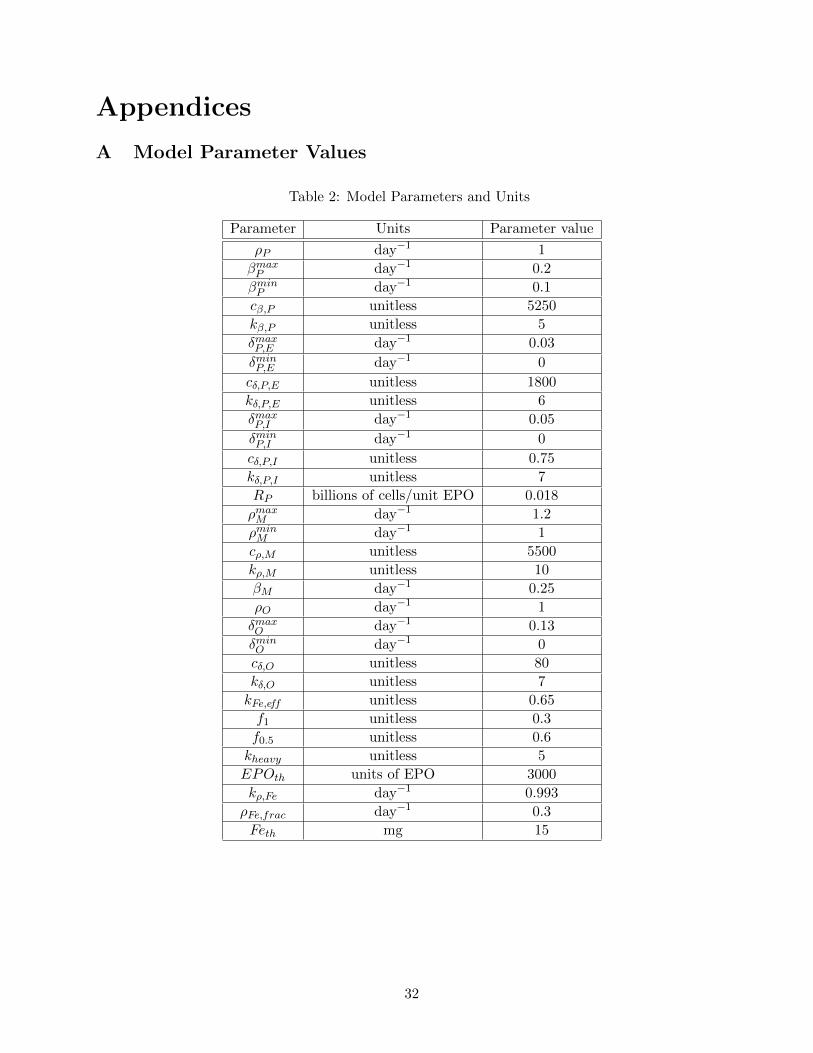
• Other parameters: The remaining parameters were given nominal values that produced ex-pected numbers of cells in classes P and M, and appropriate Hb concentrations. These param-eters could be expected to vary among individuals. The remaining nominal parameter valueswe use appear in Table 2 in Appendix A.

15 Numerical Solution Methodologies

We solve our system in a sequential manner, beginning with (13). We then solve (9) numerically, us-ing the solution of (13) in the boundary condition, (14). Similarly, use this solution in the boundarycondition (15) to solve (10), and we use the solution of (10) when we solve (11) and (12) simultane-ously. We solve using Matlab’s ode23t solver.

For equations (9), (10) and (11), we use a Galerkin finite element method. We outline thisprocedure here for class P only, but the same procedure is used for classes M and O.

Let0 = µ1 < µ2 < · · · < µNP

= µf

be a uniform partition of NP − 1 subintervals, each of length hP =µf

NP−1 . We define NP piecewiselinear continuous functions

φj , j = 1, 2, . . . , NP ,

which we will call trial solution functions, by

φj(µ) =

µ− µj−1

hP, µj−1 ≤ µ ≤ µj ,

µj+1 − µhP

, µj ≤ µ ≤ µj+1,

0, µ < µj−1 or µ > µj+1.

We will also use a set of test functions φj . Typically, the test functions are identically the sameas the trial solution functions, but choice of these test functions is discussed later.

19

We make a weak formulation of (9) by multiplying by the jth test function and integrating overall maturity levels:∫ µf

0

∂

∂tP (t, µ)φj(µ)dµ = − ρP

∫ µf

0

∂

∂µP (t, µ)φj(µ)dµ+

∫ µf

0[βP(E)− δP (E, I)]P (t, µ)φj(µ)dµ.

We assume that the solution P (t, µ) has the form

P (t, µ) =

NP∑i=1

ai(t)φi(µ), (34)

and then manipulate the resulting equation to obtain

NP∑i=1

a′i(t)

∫ µf

0φi(µ)φj(µ)dµ = − ρPaNP

(t)φj(µf ) + ρPO(t, 0)φj(0)

+

NP∑i=1

ai(t)

[ρP

∫ µf

0φi(µ)φj

′(µ)dµ

+ [βP(E)− δP (E, I)]

∫ µf

0φAi (µ)φj(µ)dµ

]. (35)

We can let j range from 1 to NP to yield a system of NP ordinary differential equations for thecoefficients ai(t). We solve this system, and reconstitute our solution using (34).

In order to validate our code, we implement a forcing function strategy. For class P, for example,we solve a modified version of (9):

∂

∂tP (t, µ) = −ρP

∂

∂µP (t, µ) + [βP (E)− δP (E, I)] P (t, µ) + F (t, µ). (36)

We choose a function such as P ∗(t, µ) = 10e−t/2 + 15e−µ/3, which is smooth and decreases tozero with increasing time and maturity level, then determine the forcing function F that guaranteesthat P ∗ is the exact solution of (36). We solve (36) numerically and compare our solution with theknown exact solution.

It is well known that the solution to (9) will propagate along its characteristic curves, which wecan think of as a “wave front.” When we use standard linear splines φj as both the trial solutionfunctions and the test functions, we introduce error at this wave front, which is propagated in time.In Figure 12a, we see that the error can become large and that standard linear splines are insufficientto resolve the solution, as described in [8]. (We will discuss the error that is similar in both Figures12a and 12b later.)

In order to alleviate this problem, we use a Petrov-Galerkin finite element method, also knownas upwinding. We continue using linear spline elements φj for the trial solution functions, but forthe test functions we use second-order functions of the form φj + ωχj , where

χj(µ) =

(µ− µj−1)(µj − µ)

h2, µj−1 ≤ µ ≤ µj ,

− (µ− µj)(µj+1 − µ)

h2, µj ≤ µ ≤ µj+1,

0, µ < µj−1 or µ > µj+1.

Figure 13 provides an example of standard test elements with varying levels of the upwinding pa-rameter ω. Note that ω = 0 corresponds to no upwinding, or standard linear spline elements.

20

(a)

(b)

Figure 12: Error with and without upwinding. Exact solution is of the order 102.

When we solve (36) numerically using nonzero values of ω, and compare our solution with theexact solution, we see significant improvement, as in Figure 12b.

We note that the small error seen in both Figure 12a and Figure 12b (that propagates along alinear characteristic from t = 0 to approximately t = 3) is due to a high order discontinuity betweenthe boundary condition and initial condition at (t, µ) = (0, 0). This error diminishes with use of afiner mesh on the structure variable.

In order to determine an appropriate value for the parameter ω, we fix the number of elementsand solve (36). Figure 14 shows the error using several values for the upwinding parameter.

0

1Test Elements φ

j + ωχ

j

ω = 0ω = 0.5ω = 1

μj μj+1μj-1 h

Figure 13: Test basis elements, with varying values of the upwinding parameter ω.

21

0 0.5 1 1.5 2 2.5 30

0.5

1

1.5

2x 10−5

maturity level, µ

erro

r

Error at t = 15 days for various levels of upwinding

ωP = 1

ωP = 1.5

ωP = 2

ωP = 2.5

ωP = 3

ωP = 3.5

Figure 14: Effect of varying ωP on error between numerical and exact solution at t = 15 for N = 256spatial elements. Exact solution is of the order 102.

We note that the error is of the same order for several values of the parameter and we choose tocontinue our simulations with ωP = 2.5 as the upwinding parameter for class P.

As one final validation of our code, we sequentially increase the number of splines elements by afactor of two to confirm that the numerical solution converges to the exact solution and to observethe rate of convergence, which is essentially quadratic. The results appear in Table 1.

We repeat this process of validating the code for classes M and O. The results appear in Appen-dices B and C.

Table 1: Convergence of Solution–Maximum Error at t = 15 with ωP = 2.5 for an increasing numberof splines. Exact solution is of the order 102.

NP Maximum error (Max Error for NP )/(Max Error for 2NP )

4 0.1298 5.2451

8 0.0247 4.5190

16 0.0055 4.2395

32 0.0013 4.1153

64 3.1384e-04 4.0566

128 7.7365e-05 4.0280

256 1.9207e-05 4.0140

512 4.7850e-06 1.7820

1024 2.6851e-06

22

16 Numerical Results and Discussion

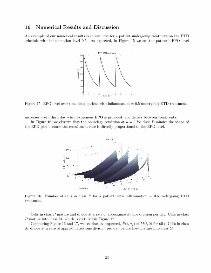
An example of our numerical results is shown next for a patient undergoing treatment on the ETDschedule with inflammation level 0.5. As expected, in Figure 15 we see the patient’s EPO level

0 1 2 3 4 5 6 7 8 90

1000

2000

3000

4000

5000

6000

time, days

units

of

EPO

EPO, ETD treatment

Figure 15: EPO level over time for a patient with inflammation = 0.5 undergoing ETD treatment.

increases every third day when exogenous EPO is provided, and decays between treatments.In Figure 16, we observe that the boundary condition at µ = 0 for class P mimics the shape of

the EPO plot because the recruitment rate is directly proportional to the EPO level.

Figure 16: Number of cells in class P for a patient with inflammation = 0.5 undergoing ETDtreatment.

Cells in class P mature and divide at a rate of approximately one division per day. Cells in classP mature into class M, which is pictured in Figure 17.

Comparing Figure 16 and 17, we see that, as expected, P (t, µf ) = M(t, 0) for all t. Cells in classM divide at a rate of approximately one division per day before they mature into class O.

23

Figure 17: Number of cells in class M for a patient with inflammation = 0.5 undergoing ETDtreatment.

As we consider Figure 18, it is worth noting that there has been a change in the time scale. Thisplot actually closely resembles the plots for classes P and M, but appears much different becauseresults are shown over a time period of 120 days as opposed to just two or three days; this is not anexample of the “noise” we discussed previously. The boundary condition, O(t, 0), is not identical toM(t, νf ) in Figure 17 because the number of cells maturing in to class O is also dependent on howmuch iron is available. Note also that cells in class O no longer divide; they simply mature and die.

Figure 18: Number of cells in class O for a patient with inflammation = 0.5 undergoing ETDtreatment.

24

0 5 10 15 20 2550

60

70

80

90

100

110

time, days

iron

, mg

Iron Level (other than in RBCs)

Figure 19: Iron level for a patient with inflammation = 0.5 undergoing ETD treatment.

The amount of iron (other than that being carried in RBCs), in Figure 19, is seen to increasegreatly when exogenous iron is introduced (on days 0 and 9). Small increases are due to iron beingrecycled from RBCs that have died.

Finally, Figure 20 shows the resulting hemoglobin concentration. The desired range, 11 to 13g/dL, is also shown.

0 5 10 15 20 2510.5

11

11.5

12

12.5

13

time, days

Hg,

g/d

L

Hemoglobin Concentration in g/dL

Figure 20: Hemoglobin concentration for a patient with inflammation = 0.5 undergoing ETD treat-ment.

25

Figure 21 shows similar results for a patient at inflammation level 0.5 undergoing MWF treatment.

0 2 4 6 8 10 12 141000

2000

3000

4000

5000

6000

7000

time, days

units

of

EPO

EPO, MWF treatment

0 2 4 6 8 10 12 14 16 18 2040

50

60

70

80

90

100

110

time, days

iron

, mg

Iron Level (other than in RBCs)

0 2 4 6 8 10 12 14 16 18 2010

10.5

11

11.5

12

12.5

13

time, days

Hg,

g/d

L

Hemoglobin Concentration in g/dL

Figure 21

26

0 2 4 6 8 10 12 14 16 189

9.5

10

10.5

11

11.5

12

12.5

13

time, days

hem

oglo

bin

conc

, g/d

L

Hb concentration with varying inflammation

infl = 0

infl = 0.25

infl = 0.5

infl = 0.75

infl = 1

0 2 4 6 8 10 12 14 16 1820

40

60

80

100

120

140

160

180

time, days

mg

of ir

on

Iron (other than in RBCs) with varying inflammation

infl = 0

infl = 0.25

infl = 0.5

infl = 0.75

infl = 1

Figure 22: Hemoglobin concentration and iron with varying inflammation, ETD treatment.

0 2 4 6 8 10 12 148.5

9

9.5

10

10.5

11

11.5

12

12.5

13

time, days

hem

oglo

bin

conc

, g/d

L

Hb concentration with varying inflammation

infl = 0

infl = 0.25

infl = 0.5

infl = 0.75

infl = 1

0 2 4 6 8 10 12 1420

40

60

80

100

120

140

160

time, days

mg

of ir

on

Iron (other than in RBCs) with varying inflammation

infl = 0

infl = 0.25

infl = 0.5

infl = 0.75

infl = 1

Figure 23: Hemoglobin concentration and iron with varying inflammation, MWF treatment.

We also present some results of varying the inflammation level for both ETD (Figure 22) andMWF treatment (Figure 23).

It should be noted here that the solutions are dependent on the initial conditions, and thereforecareful choice of initial conditions must be made in order to produce results that biologically rea-sonable. For example, if one starts with an an initial condition O(t, 0) that is large, then the ironbeing carried in those cells eventually ends up in the iron compartment, which in turn affects therecruitment rate into class O. As a result, it is possible, for example, to produce a set of simulationssuch that the hemoglobin concentration for a patient with inflammation level 0.5 is actually higherthan for a patient with a lower inflammation level.

For each treatment protocol, we also compare iron needed, Feneeded and iron available, Feavail,over time at various levels of inflammation so that we might understand the dynamics of iron indetermining the number of cells maturing in to class O (see Figures 24 and 25). It is worth notingagain that the solutions (in particular iron available) are dependent on the initial conditions.

27

0 2 4 6 8 10 12 14 16 180

20

40

60

80

100

120

time, days

mg

of ir

onIron available Compared with Iron Needed, inflammation = 0

AvailableNeeded

0 2 4 6 8 10 12 14 16 180

20

40

60

80

100

120

time, days

mg

of ir

on

Iron available Compared with Iron Needed, inflammation = 0.25

AvailableNeeded

0 2 4 6 8 10 12 14 16 180

20

40

60

80

100

120

time, days

mg

of ir

on


AvailableNeeded

0 2 4 6 8 10 12 14 16 180

20

40

60

80

100

120

time, daysm

g of

iron


AvailableNeeded

0 2 4 6 8 10 12 14 16 180

20

40

60

80

100

120

time, days

mg

of ir

on

Iron available Compared with Iron Needed, inflammation = 1

AvailableNeeded

Figure 24: Feneeded and Feavail with varying inflammation, ETD treatment.

17 Summary

The model presented is capable of describing patients over a broad range of conditions, includingvarious inflammation levels and treatment protocols. Parameter values were prescribed per theliterature, when available, and numerical testing validates the use of our code in solving the model.Some numerical results are presented, making note that the results are highly dependent on theinitial conditions, which are estimated.

This model makes significant simplifications with regard to how iron is assimilated into red bloodcells. As such, the next step will be to revisit the model to determine a more biologically reasonableway to incorporate iron, perhaps through the use of another structure variable which will accountfor the amount of iron in a cell.

This paper did not attempt to address the concept of iron homeostasis, but it is also becomingmore and more evident that understanding iron homeostasis will play a role in this model’s abilityto predict the outcomes of treatment protocols. It appears that hepcidin production is regulated,

28

0 2 4 6 8 10 12 140

10

20

30

40

50

60

70

80

90

100

time, days

mg

of ir

onIron available Compared with Iron Needed, inflammation = 0

AvailableNeeded

0 2 4 6 8 10 12 140

10

20

30

40

50

60

70

80

90

100

time, days

mg

of ir

on


AvailableNeeded

0 2 4 6 8 10 12 140

10

20

30

40

50

60

70

80

90

100

time, days

mg

of ir

on


AvailableNeeded

0 2 4 6 8 10 12 140

10

20

30

40

50

60

70

80

90

100

time, daysm

g of

iron


AvailableNeeded

0 2 4 6 8 10 12 140

10

20

30

40

50

60

70

80

90

100

time, days

mg

of ir

on

Iron available Compared with Iron Needed, inflammation = 1

AvailableNeeded

Figure 25: Feneeded and Feavail with varying inflammation, MWF treatment.

at least in part, by the rate of erythropoiesis [5], but hepcidin has only recently been discovered asthe major regulator of iron homeostasis, and therefore its action is only partially understood as thebody of literature on hepcidin is relatively small.

This model does address, for the first time, the roles inflammation and iron play in red blood celldynamics, which are known to have a significant impact on red blood cell dynamics in patients withCKD.

Acknowledgements

This research was supported in part by Grant Number R01AI071915-07 from the National Insti-tute of Allergy and Infectious Diseases.

29

References

[1] A. Ackleh, K. Deng, K. Ito, and J. Thibodeaux. A structured erythropoiesis model with non-linear cell maturation velocity and hormone decay rate. Mathematical Biosciences, 204(1):21 –48, 2006.

[2] Suhail Ahmad. Manual of Clinical Dialysis, Second Edition. Springer Science + Business Media,LLC, New York, 2009.

[3] H. T. Banks, C. Cole, P. Schlosser, and H. T. Tran. Modeling and optimal regulation of erythro-poiesis subject to benzene intoxication. Mathematical Biosciences and Engineering, 1(1):15–48,2004.

[4] J. Belair, M. Mackey, and J. Mahaffy. Age-structured and two-delay models for erythropoiesis.Mathematical Biosciences, 128(1-2):317 – 346, 1995.

[5] Tomas Ganz. Iron homeostasis: Fitting the puzzle pieces together. Cell Metabolism, 7:288–290,2008.

[6] L. Israels and E. Israels. Erythropoiesis: an overview. In Erythropoietins and Erythropoiesis:Molecular, Cellular, Preclinical and Clinical Biology, pages 3–14. Birkhauser Verlag, 2003.

[7] W. Jelkmann. Erythropoietin: structure, control of production, and function. Physiologicalreviews, 72(2):449–489, 1992.

[8] Shengtai Li and Linda Petzold. Moving mesh methods with upwinding schemes for time-dependent pdes. Journal of Computational Physics, 131:368–377, 1997.

[9] I. Macdougall. Use of recombinant erythropoietins in the setting of renal disease. In S.G. ElliotG. Molineaux, M.A. Foote, editor, Erythropoietins and Erythropoiesis: Molecular, Cellular,Preclinical and Clinical Biology, pages 153–159. Birkhauser Verlag, 2003.

[10] I. Macdougall and A. Cooper. Erythropoietin resistance: the role of inflammation and pro-inflammatory cytokines. Nephrol. Dial. Transplant., 17:39–43, 2002.

[11] J. Mahaffy, J. Belair, and M. Mackey. Hematopoietic model with moving boundary condi-tion and state dependent delay: applications in erythropoiesis. Journal of Theoretical Biology,190(2):135–146, 1998.

[12] R. Means Jr. and S. Krantz. Inhibition of human erythroid colony-forming units by interfer-ons alpha and beta: differing mechanisms despite shared receptor. Experimental Hematology,24(2):204–208, 1996.

[13] National Kidney Foundation Kidney Disease Outcomes Quality Initiative. KDOQI ClinicalPractice Guidline and Clinical Practive Recommendations for Anemia in Chronic Kidney Dis-ease: 2007 Update of Hemoglobin Target. American Journal of Kidney Diseases, 50(3):471–530,2007.

[14] R. Ramakrishnan, W. Cheung, M. Wacholtz, N. Minton, and W. Jusko. Pharmacokinetic andpharmacodynamic modeling of human erythropoietin after single and multiple doses in healthyvolunteers. The Journal of Clinical Pharmacology, 44:991–1002, 2004.

[15] A. Simmons. Basic Hematology. Charles C Thomas, Springfield, Illinois, 1973.

30

[16] P. Stenvinkel. The role of inflammation in the anaemia of end-stage renal disease. Nephrology,Dialysis, Transplantation, 16(Suppl 7):36–40, 2001.

[17] U.S. Renal Data System. USRDS 2008 Annual Data Report: Atlas of Chronic Kidney Diseaseand End-Stage Renal Disease in the United States. National Institutes of Health, NationalInstitute of Diabetes and Digestive and Kidney Diseases, Bethesda, MD, 2008.

[18] S. Woo, W. Krzyzanski, and W. Jusko. Pharmacokinetic and pharmacodynamic modeling ofrecombinant human erythropoietin after intravenous and subcutaneous administration in rats.Journal of Pharmacology and Experimental Therapeutics, 319(3):1297–1306, 2006.

31

Appendices

A Model Parameter Values

Table 2: Model Parameters and Units

Parameter Units Parameter value

ρP day−1 1

βmaxP day−1 0.2

βminP day−1 0.1

cβ,P unitless 5250

kβ,P unitless 5

δmaxP,E day−1 0.03

δminP,E day−1 0

cδ,P,E unitless 1800

kδ,P,E unitless 6

δmaxP,I day−1 0.05

δminP,I day−1 0

cδ,P,I unitless 0.75

kδ,P,I unitless 7

RP billions of cells/unit EPO 0.018

ρmaxM day−1 1.2

ρminM day−1 1

cρ,M unitless 5500

kρ,M unitless 10

βM day−1 0.25

ρO day−1 1

δmaxO day−1 0.13

δminO day−1 0

cδ,O unitless 80

kδ,O unitless 7

kFe,eff unitless 0.65

f1 unitless 0.3

f0.5 unitless 0.6

kheavy unitless 5

EPOth units of EPO 3000

kρ,Fe day−1 0.993

ρFe,frac day−1 0.3

Feth mg 15

32

B Code validation for class M

As in class P, we note that if we don’t use upwinding, the error can propagate in time and overwhelmthe solution, as demonstrated by comparing the numerical solutions for class M (using the forcingprocedure described perviously) with and without upwinding, as in Figures 26a and 26b.

(a) (b)


In order to determine an appropriate value for the parameter ωM , we fix the number of elementsand compare the error using several values for the upwinding parameter.

0 0.5 1 1.5 2 2.5 30

1

2

3

4

5

6

7

8

9x 10

−6

maturity level, μ

erro

r


ωM

= 0.5

ωM

= 1

ωM

= 1.5

ωM

= 2

ωM

= 2.5

ωM

= 3

Figure 27: Effect of varying ωM on error between numerical and exact solution at t = 15 for N = 256spatial elements. Exact solution is of the order 102.

We note that the error is of the same order for several values of the parameter and we choose tocontinue our simulations with ωM = 2 as the upwinding parameter for class M.

As before, we sequentially increase the number of splines elements by a factor of two to confirmthat the numerical solution converges to the exact solution. The results appear in Table 3.

33

Table 3: Convergence of Solution–Maximum Error at t = 15 with ωM = 2 for an increasing numberof splines. Exact solution is of the order 102.

NM Maximum error (Max Error for NM )/(Max Error for 2NM )

4 0.0614 5.4641

8 0.0112 4.5726

16 0.0025 4.2623

32 5.7693e-04 4.1259

64 1.3983e-04 4.0617

128 3.4427e-05 1.0000

256 3.4427e-05 16.1836

512 2.1273e-06 2.4047

1024 8.8464e-07

C Code validation for class O

Unlike classes P and M , at time t = 15 days, in Figure 28 we are not able to see the error over-whelming the solution without the use of upwinding.

(a) (b)


It appears there may not be an advantage to using upwinding in this case. We continue in-vestigating by fixing the number of elements and comparing the error using several values of theupwinding parameter ωO.

We note that the error is of the same order for several values of the parameter, including for noupwinding. We choose to continue our simulations with upwinding (for consistency with the otherclasses), using ωO = 3.5 as the upwinding parameter for class O.

As before, we sequentially increase the number of splines elements by a factor of two to confirmthat the numerical solution converges to the exact solution. The results appear in Table 4.

34

0 20 40 60 80 100 120−6

−4

−2

0

2

4

6x 10

−4

maturity level, ψ

erro

r


ωO

= 0

ωO

= 1

ωO

= 2

ωO

= 3

ωO

= 3.5

ωO

= 4

Figure 29: Effect of varying ωO on error between numerical and exact solution at t = 15 for N = 1201spatial elements. Exact solution is of the order 102.

Table 4: Convergence of Solution–Maximum Error at t = 15 with ωO = 3.5 for an increasing numberof splines. Exact solution is of the order 102.

NM Maximum error (Max Error for NO)/(Max Error for 2NO)8 4.6086 2.6825

16 1.7180 3.1906

32 0.5385 3.5164

64 0.1531 3.7385

128 0.0410 3.8632

256 0.0106 3.9299

512 0.0027 3.9645

1024 6.8052e-04 3.9821

2048 1.7089e-04 3.9911

4096 4.2819e-05

35

a computational model of red blood cell dynamics in patients with

Documents