Institute of Structural Mechanics

A comprehensive study: Boundary conditions for representative volume elements (RVE) of composites

Srihari Kurukuri

A technical report on homogenization techniques

A comprehensive study: Boundary conditions for representative

volume elements (RVE) of composites

Abstract A comprehensive study has been carried out on the effect of different types of boundary conditions imposed on the RVE to predict the effective properties of heterogeneous materials through the concept of homogenization. In this study three types of boundary conditions were presented namely: displacement-difference periodic boundary conditions, homogeneous boundary conditions and prescribed displacements boundary conditions. It has been realized that, with in numerical accuracy, the effective properties under periodic boundary conditions and prescribed displacement boundary conditions are the same and it can easily be applied in FE analysis even when compared with the periodic boundary conditions. It has been demonstrated that the homogeneous boundary conditions are not only over-constrained but they may also violate the traction periodicity conditions. Further it is deduced that boundary traction continuity conditions can be guaranteed by the application of the proposed displacement-difference periodic boundary conditions and prescribed boundary conditions. Illustrative examples are presented.

1. Introduction Composite materials are widely used in advanced structures in astronautics, automobile, marine,

petrochemical and many other industries due to their superior properties over conventional

engineering materials. Consequently, prediction of the mechanical properties of the composites

has been an active research area for several decades. Except for the experimental studies, either

micro- or macro mechanical methods are used to obtain the overall properties of composites.

Micromechanical method provides overall behavior of the composites from known properties of

their constituents (fiber and matrix) through an analysis of a representative volume element

(RVE) or a unit-cell model (Aboudi, 1991; Nemat-Nasser and Hori, 1993). In the

macromechanical approach, on the other hand, the heterogeneous structure of the composite is

replaced by a homogeneous medium with anisotropic properties. The advantage of the

micromechanical approach is not only the global properties of the composites but also various

mechanisms such as damage initiation and propagation, can be studied through the analysis

There are several micromechanical methods used for the analysis and prediction of the overall

behavior of composite materials. In particular, upper and lower bounds for elastic moduli have

been derived using energy variational principles, and closed-form analytical expressions have

been obtained (Hashin and Shtrikman, 1963; Hashin and Rosen, 1964). Unfortunately, the

generalization of these methods to viscoelastic, elastoplastic and nonlinear composites is very

difficult. Aboudi (1991) has developed a unified micromechanical theory based on the study of

interacting periodic cells, and it was used to predict the overall behavior of composite materials

both for elastic and inelastic constituents. In his work and many other references, homogeneous

boundary conditions were applied to the RVE or unit cell models. In fact, the ‘‘plane-remains-

1

plane’’ is only valid for the symmetric RVE subjected to normal tractions. For a shear loading

case, many researchers, have indicated that the plane-remains-plane boundary conditions are

over-constrained boundary conditions.

In this article, a comprehensive study has been carried out on the effect of different types of

boundary conditions imposed on the RVE to predict the effective properties of heterogeneous

materials through the concept of homogenization. In this study three types of boundary conditions

were presented namely: displacement-difference periodic boundary conditions, homogeneous

boundary conditions and prescribed displacements boundary conditions.

2. Theoretical background In this work, three types of boundary conditions to be prescribed on individual volume element V

are considered namely:

1. Homogenous boundary conditions

2. Periodic boundary conditions

3. Prescribed displacement boundary conditions.

2.1. Homogeneous boundary conditions Aboudi (1991) applied on the surface of a homogeneous body will produce a homogeneous field

there. Such boundary conditions are obtained in the form:

• Kinematic uniform boundary conditions (KUBC):The displacement u is imposed at

point x belonging to the boundary such that: S

jiji xSu 0)( ε= , Sx∈∀ (1)

0ijε is constant and symmetrical second rank tensor that does not depend on x .

• Static uniform boundary conditions (SUBC): The traction vector is prescribed at the

boundary:

, jiji nSt 0)( σ= Sx∈∀ (2)

is a constant and symmetrical second rank tensor independent of 0ijσ x . The vector

normal to at S x is denoted by . n

2.2. Periodic boundary conditions Consider a periodic structure consisting of periodic array of repeated unit cells. The displacement

field for the periodic structure can be expressed as

),,(),,( 321*0

321 xxxuxxxxu ijiji += ε (3)

2

In the above, is the global (average) strain tensor of the periodic structure and the first term

on the right side represents a linear distributed displacement field. The second term on the right

side, is a periodic function from one unit cell to another. It represents a

modification to the linear displacement field due to the heterogeneous structure of the

composites.

0ijε

),,( 321* xxxui

Since the periodic array of the repeated unit cells represents a continuous physical body, two

continuities must be satisfied at the boundaries of the neighboring unit cells. One is that the

displacements must be continuous, i.e., the adjacent unit cells cannot be separated or intrude into

each other at the boundaries after the deformation. The second condition implies that the traction

distributions at the opposite parallel boundaries of a unit cell must be the same. In this manner,

the individual unit cell can thus be assembled as a physically continuous body.

Obviously, the assumption of displacement field in the form of Eq. (3) meets the first of the above

requirements. Unfortunately, it cannot be directly applied to the boundaries since the periodic

part, is generally unknown. For any unit cell, its boundary surfaces must always

appear in parallel pairs, the displacements on a pair of parallel opposite boundary surfaces can

be written as

),,( 321* xxxui

*0i

kjij

ki uxu += ++ ε (4)

*0i

kjij

ki uxu += −− ε (5)

where indices ‘‘ ’’ and ‘‘ ’’ identify the k+k −k th pair of two opposite parallel boundary surfaces of a repeated unit cell. Note that is the same at the two parallel boundaries (periodicity), therefore, the difference between the above two equations is

),,( 321* xxxui

kjij

kj

kjik

ki

ki xxxuu Δ=−=− −+−+ 00 )( εε (6)

Since are constants for each pair of the parallel boundary surfaces, with specified , the

right side becomes constants and such equations can be easily be applied in the finite element

analysis as nodal displacement constraint equations. Eq. (6) is a special type of displacement

boundary conditions. Instead of giving known values of boundary displacements, it specifies the

displacement-differences between two opposite boundaries. Obviously, the application of it will

guarantee the continuity of displacement field. However, in general, such displacement-difference

boundary conditions, Eq. (6), may not be complete or may not guarantee the traction continuity

conditions. The traction continuity conditions can be written as

kjxΔ 0

ijε

,0=− −+ kn

kn σσ (7) 0=− −+ k

tkt σσ

3

where and are normal and shear stresses at the corresponding parallel boundary

surfaces, respectively. For general periodic boundary value problems the Eqs. (6) and (7)

constitute a complete set of boundary conditions.

nσ tσ

In the following illustrative examples, however, it has been proved that if unit cell is analyzed by

using a displacement-based finite element method, the application of only Eq. (6) can guarantee

the uniqueness of the solution and thus Eq. (7) are automatically satisfied. In other word, the

latter boundary conditions are not necessary to be applied in the analysis.

2.3. Prescribed displacement boundary conditions These boundary conditions have to be applied to the RVE in such a way that, except the strains

in the direction, in which the effective coefficients have to be calculated, all other mechanical

strains are zero. As a load, uniform unidirectional displacement (prescribed displacement

condition) is applied.

As an example: To find the effective coefficients and the boundary conditions have to be

applied to the RVE in such a way that, except the strain in the X direction, all other global strains

are set to zero. As a load, uniform unidirectional displacement (prescribed displacement

condition) is applied on the positive X-edge. The displacements in normal direction on the positive

and negative Y-edges are constrained to be zero. So that the strain in the X-direction is the only

one, having finite value and all other strains are set to be zero. It has been observed that the

effective properties obtained under our prescribed displacement boundary conditions and periodic

boundary conditions are the same with in numerical accuracy.

11C 12C

3. 3. Numerical homogenization using RVE FEM has been extensively used in the literature to analyze unit cell, to determine the mechanical

properties and damage mechanisms of composites. In the present work the FEM

micromechanical analysis method is applied to periodic RVE. For simplicity, all the following

illustrative examples are 2–D plane stress state problems considered. All finite element

calculations have been carried out with commercial FE program ANSYS. To apply the constraint

equations (6) in FEM, it is better to produce the same meshing at each two paired boundary

surfaces. Then each constraint equation in (6) contains only two displacement components of the

paired nodes. The number of the constraint equations is usually quite large, certain preprocessing

program can be used to produce the data depending on the individual FEM code used. In all

following FEM analyses six node plane stress elements are used with small deformation

assumption. The convergence of the solutions has been verified by comparing the results with

different meshing sizes.

4

It is assumed that the average mechanical properties of a RVE are equal to the average

properties of the particular composite material. The average stresses and strains in a RVE are

defined by:

∫=V ijij dV

Vεε 10 (8)

∫=V ijij dV

Vσσ 10 (9)

In order to evaluate the effective properties , first we should evaluate the average stress and

average strain, from the Eqs. (8) and (9) with the application of different boundary conditions, and

then insert them into the constitutive relation as follows:

ijklC

kl

ijijklC

εσ

= (10)

In numerical analysis of RVE, stress, strain have been taken from each and every element and

multiplied with the volume of each element and then finally compute the averaged stresses and

strains over all elements.

The strain energies predicted by the different boundary conditions must satisfy the following

inequality if the average strain for each case is assumed to be the same (Suquet, 1987; Hori

and Nemat-Nasser, 1999; Hollister and Kikuchi, 1992):

0ijε

dpt UUU ≤≤ (11)

where are the strain energy predicted by homogeneous traction boundary conditions,

periodic boundary conditions, and homogeneous displacement boundary conditions, respectively.

It is clear that the homogeneous displacement boundary conditions overestimate the effective

moduli whereas the homogeneous traction boundary conditions underestimate the effective

moduli. It is also being pointed out that the application of the homogeneous displacement

boundary conditions generally would not guarantee to produce periodic boundary traction.

Similarly, the application of the homogeneous traction boundary conditions would not guarantee

the displacement periodicity at the boundaries.

dpt UUU ,,

4. Results and discussion The results obtained from the proposed displacement difference periodic boundary conditions

and prescribed displacement boundary conditions, with those obtained by applying homogeneous

boundary conditions are compared. Consider the periodic structure as shown in Fig. 1. The

volume fraction of the reinforcing phase is 20 %. Assume both reinforcing and matrix phases are

elastic and their material constants are:

MPaE f 85000= , 25.=fν and MPaEm 2800= , 4.=mν respectively.

5

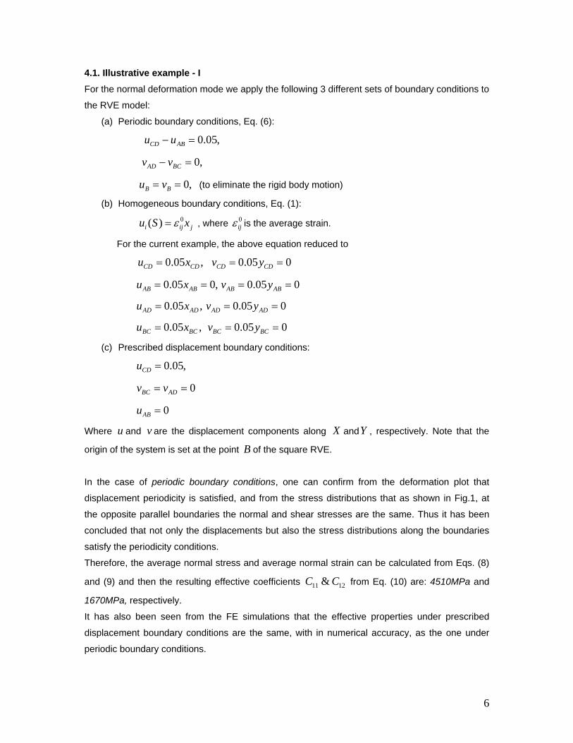
4.1. Illustrative example - I For the normal deformation mode we apply the following 3 different sets of boundary conditions to

the RVE model:

(a) Periodic boundary conditions, Eq. (6):

,05.0=− ABCD uu

,0=− BCAD vv

(to eliminate the rigid body motion) ,0== BB vu

(b) Homogeneous boundary conditions, Eq. (1):

, where is the average strain. jiji xSu 0)( ε= 0ijε

For the current example, the above equation reduced to

,05.0 CDCD xu = 005.0 == CDCD yv

,005.0 == ABAB xu 005.0 == ABAB yv

,05.0 ADAD xu = 005.0 == ADAD yv

,05.0 BCBC xu = 005.0 == BCBC yv

(c) Prescribed displacement boundary conditions:

,05.0=CDu

0== ADBC vv

0=ABu

Where and are the displacement components along u v X andY , respectively. Note that the

origin of the system is set at the point B of the square RVE.

In the case of periodic boundary conditions, one can confirm from the deformation plot that

displacement periodicity is satisfied, and from the stress distributions that as shown in Fig.1, at

the opposite parallel boundaries the normal and shear stresses are the same. Thus it has been

concluded that not only the displacements but also the stress distributions along the boundaries

satisfy the periodicity conditions.

Therefore, the average normal stress and average normal strain can be calculated from Eqs. (8)

and (9) and then the resulting effective coefficients from Eq. (10) are: 4510MPa and

1670MPa, respectively.

1211 & CC

It has also been seen from the FE simulations that the effective properties under prescribed

displacement boundary conditions are the same, with in numerical accuracy, as the one under

periodic boundary conditions.

6

(a)

XY

(b) (c) Fig.1. FEM solution of RVE by applying periodic boundary conditions - Normal coefficient: (a) deformation ; (b) stress xu xσ (MPa); (c) stress xyτ (MPa)

In the case of homogeneous displacement boundary conditions, it can be seen from deformation

plot that displacement periodicity is satisfied, but from the shear stress distribution it can be seen

that along the X-direction, on positive and negative boundaries the shear stresses are not the

same. Thus it can be implied that traction distributions along the boundaries does not satisfy the

periodicity conditions, i.e. Eq. (7) is not satisfied.

Therefore, the average normal stress and average normal strain can be calculated from Eqs. (8)

and (9) and then the resulting effective coefficients from Eq. (10) are: 4534MPa and

1665MPa, respectively.

1211 & CC

7

(a)

XY

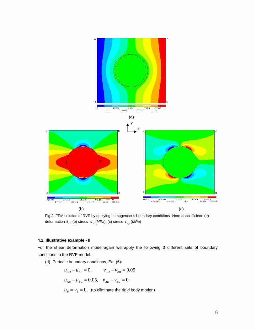
(b) (c) Fig.2. FEM solution of RVE by applying homogeneous boundary conditions- Normal coefficient: (a) deformation ; (b) stress xu xσ (MPa); (c) stress xyτ (MPa)

4.2. Illustrative example - II For the shear deformation mode again we apply the following 3 different sets of boundary

conditions to the RVE model:

(d) Periodic boundary conditions, Eq. (6):

,0=− ABCD uu 05.0=− ABCD vv

,05.0=− BCAD uu 0=− BCAD vv

(to eliminate the rigid body motion) ,0== BB vu

8

(e) Homogeneous boundary conditions, Eq. (1):

, where is the average strain. jiji xSu 0)( ε= 0ijε

For the current example, the above equation reduced to

,05.0 CDCD yu = 05.005.0 == CDCD xv

,05.0 ABAB yu = 005.0 == ABAB xv

,05.0 ADAD yu = ADAD xv 05.0=

,005.0 == BCBC yu BCBC xv 05.0=

(f) Prescribed displacement boundary conditions:

05.0−=ABv

,05.0=CDv

05.0−=BCu

05.0=ADu

Where and are the displacement components along u v X andY , respectively. Note that the

origin of the system is set at the point B of the square RVE.

The deformed shape for the case of periodic boundary conditions is shown in Fig. 3 (a). One

notes that the boundaries do not remain planes after the deformation. Further assessment of the

stress distribution indicates that at all opposite corresponding boundaries the normal and shear

stress are the same as shown in Figs. 3 (b) and (c), i.e. the RVE is subjected to pure shear load.

In addition, not only the displacements but also the stress distributions along the boundaries

satisfy the periodicity conditions.

Therefore, the average normal stress and average normal strain can be calculated from Eqs. (8)

and (9) and then the resulting effective coefficient from Eq. (10) is: 1309MPa. 66C

It has also been seen from the FE simulations that the effective properties under prescribed

displacement boundary conditions are the same, with in numerical accuracy, as the one under

periodic boundary conditions.

9

(a)

(b) (c)

Fig.3. FEM solution of RVE by applying periodic boundary conditions - shear coefficient: (a) deformation ; (b) stress xu xσ (MPa); (c) stress xyτ (MPa)

In contrast, Fig.4 shows the results by applying the plane-remains-plane (homogeneous

displacement) boundary conditions. The boundary lines remain straight lines. Therefore, the

displacement periodicity is satisfied, but one can see that the normal stresses at the

corresponding parallel boundaries are not the same, i.e. the traction continuity conditions, Eq. (7),

is violated and therefore this distribution of stresses cannot represent the real one of physically

continued periodic structure. Accordingly, it is clear that the homogeneous displacement

boundary conditions are not appropriate boundary conditions for the RVE of composite materials

subjected to a shear load.

Therefore, the average normal stress and average normal strain can be calculated from Eqs. (8)

and (9) and then the resulting effective coefficient from Eq. (10) is: 1401MPa. We can see 66C

10

that the homogeneous displacement boundary condition does overestimate the effective

coefficient.

(a)

(b) (c)

Fig.4. FEM solution of RVE by applying homogeneous boundary conditions - shear coefficient: (a) deformation ; (b) stress xu xσ (MPa); (c) stress xyτ (MPa)

Conclusions: The following conclusions have been drawn from the present study:

• A comprehensive study has been carried out on the effect of different types of

boundary conditions imposed on the RVE to predict the effective properties of

heterogeneous materials through the concept of homogenization. In this study three

types of boundary conditions were presented namely: displacement-difference

periodic boundary conditions, homogeneous boundary conditions and prescribed

displacements boundary conditions.

11

• The proposed explicit form of displacement-difference periodic boundary conditions

for repetitive unit cell model can easily be applied in FE analysis as a set of constraint

equations of nodal displacements of corresponding nodes on the opposite parallel

boundary surfaces of the RVE.

• The application of the periodic boundary conditions and prescribed displacement

boundary conditions can guarantee the displacement continuity and traction

continuity at the boundaries of the RVE and as such it is the solution for real periodic

structure.

• It has also been seen from the FE simulations that the effective properties under

prescribed displacement boundary conditions are the same, with in numerical

accuracy, as the one under displacement-difference periodic boundary conditions

and can easily be applied in FE analysis even when compared with the periodic

boundary conditions.

• The homogeneous boundary conditions (plane-remain-plane) are not only over-

constrained conditions but they may also violate the stress periodicity. This type of

boundary conditions shows a great discrepancy in effective properties when applying

the shear loading.

References 1. Aboudi, J., 1990. Micromechanical prediction of initial and subsequent yield surfaces of metal matrix composites. International Journal of Plasticity 6, 134–141. 2. Aboudi, J., 1991. Mechanics of Composite Materials, A Unified Micromechanical Approach. Elsevier Science Publishers, Amsterdam. 3. Hashin, Z., Shtrikman, S., 1963. A variational approach to the theory of elastic behavior of multiphase materials. Journal of Mechanics and Physics of Solids 11, 127–140. 4. Hashin, Z., Rosen, B.W., 1964. The elastic moduli of fiber-reinforced materials. ASME Journal of Applied Mechanics 31, 223–232. 5. Nemat-Nasser, S., Hori, M., 1993. Micromechanics: Overall Properties of Heterogeneous Materials. Elsevier Science Publishers, Amsterdam. 6. Sun, C.T., Vaidya, R.S., 1996. Prediction of composite properties from a representative volume element. Composite Science and Technology 56, 171–179. 7. Xia, Z., Zhang, Y., Ellyin, F., 2003. A unified periodical boundary conditions for representative volume elements of composites and applications. International Journal of Solids and Structures 40, 1907–1921.

12