a complete set of radiative and auger rates for k-vacancy … · 2013-04-10 · 2 p. palmeri et...
TRANSCRIPT

/%: >lioii y & Astrophysics manuscript no. paper2’5 November 25,2002 r- (DOI: will be inserted by hand later)
A Complete Set of Radiative and Auger Rates for K-vacancy States in Fe xvm-Fe xxv
P. Palmeri’**, C. Mendoza’***, T. R. Kallman’, and M. A. Bautista2
’ NASA Goddard Space Flight Center, Code 662, Greenbelt, MD 20771, USA Centro de Fisica, Instituto Venezolano de Investigaciones Cientificas (IVIC), PO Box 21827, Caracas 1020A, Venezuela
Received ;Accepted
Abstract. A complete set of level energies, wavelengths, A-values, and total and partial Auger rates have been computed for transitions involving the K-vacancy states within the n = 2 complex of Fe xvm-Fe xxv. Three different standard numerical packages are used for this purpose, namely AUTOSTRUCTURE, the Breit-Pauli R-matrix suite (BPRM) and HFR, which allow reliable estimates of the physical effects involved and of the accuracy of the resulting data sets. It is found that the Breit interaction must be always taken into account as the contributions to the small A-values and partial Auger rates does not decrease with electron occupancy. Semi-empirical adjustments can also lead to large differences in both the radiative and Auger decay data of strongly mixed levels. Several experimental energy levels and wavelengths are questioned, and significant discrepancies are found with previously computed decay rates that are attributed to numerical problems. The statistical accuracy of the present level energies and wavelengths is ranked at *3 eV and *2 d, respectively, whereas that for A-values and partial Auger rates greater than lOI3 s-’ is estimated at better than 20%.
Key words. atomic data - atomic processes -X-rays: spectroscopy
1. Introduction
We are currently involved in a project to calculate accurate atomic data for the modeling of iron K lines. It has been mo- tivated by the diagnostic potential of these lines in the X-ray spectra of high energy environments (quasars, active galactic nuclei, galactic black-hole candidates) which are now being fo- cused by powerful satellite-borne telescopes (Chandm, XMM- Newton) and will gain greater importance with the launch of the Astro-E2 telescope. In an earlier report on the decay prop- erties of the K-vacancy states in Fe XXIV (Bautista et al. 2002), to be referred hereafter as Paper I, a numerical approach was established that has led to data sets of A-values and Auger rates firmly ranked with accuracy 161.5%. It relies on calculations with several general-use computational atomic physics codes and extensive comparisons with previous work. A formal treat- ment of the Breit interaction was emphasized then in the case of the distinctively magnetic Fe Li-like ion, leading to critical evaluations of the effectiveness of the different computational packages in the treatment of inner-shell processes and of the quality previously available data.
The method of Paper I is here extended to generate a com- plete set of energy levels, wavelengths, A-values and Auger
rates for all the K-vacancy states of the n = 2 complex in Fe xxv-Fe xvm. In this respect, the critical compilation by Shirai et al. (2000) certifies the current incompleteness of the inner-shell level structures of Fe ions which is a major obstacle in line identification and spectral modeling in the above men- tioned astrophysical endeavors. Although the precision of com- puted wavelengths does not match measurements by an order of magnitude, as shown in Paper I, an exhaustive and reason- ably accurate (e.g. - 1 mA) inventory will certainly facilitate spectroscopic identifications, be an asset in the resolution of line,blends and lead to further structural refinement. A survey of the radiative and autoionization data for Fe ions with elec- tron occupancies N 5 6 computed by Chen (1986), Chen & Crasemann (1987, 1988), Chen et al. (1997) and those con- tained in the “Cornille” and “Safronova” data sets compiled by Kato et al. (1997) results in notable discrepancies that under- mine confidence in spectral modeling. For ions with N > 6 there has hardly been any attention. A-values for the allowed and forbidden valence-valence transitions within the n = 2 complex have also been included since the the post-Auger ra- diative signature, rich in UV and optical emission lines, has been shown to have astrophysical potential (Shapiro & Bahcall 1981).
Send offprint requests to: T.R. Kallman, e-mail: [email protected]
Research Associate, Department of Astronomy, University of Maryland, College Park, MD 20742 ** Present address: Centro de Fisica, IVIC, Caracas 1020A
The details of the computational approach. and of the ap- proximations considered are given in Sections 2-3, as well as those of previously available data sets that are brought in for comparison purposes. Results, namely energy levels, A-values
https://ntrs.nasa.gov/search.jsp?R=20030022794 2020-04-14T11:28:59+00:00Z

2 P. Palmeri et al.: Rates for K-vacancy States in Fe XVIII - xxv
and Auger rates, are discussed in Sections 4-6 ending with a summary and conclusions in Section 7. 1 2. Numerical methods
The present computational approach is based on standard atomic physics codes, namely AUTOSTRUCTURE, HFR, and BPRM, rather than on in-house developments. They have been widely used in the past thirty years to study valence-electron processes and more recently to the inner shells. These packages allow the inclusion of electron-correlation effects, core relaxation, rela- tivistic corrections and semi-empirical fine tuning. Radiative and collisional data are computed for N - or ( N + 1)-electron systems in a relativistic Breit-Pauli framework
~
H b p = Hnr + Hlb 4- H2b (1)
where H , is the usual non-relativistic Hamiltonian. The one- body relativistic operators
represent the spin-orbit interaction, fn(so), and the non- fine structure mass-variation, fn(mass), and one-body Darwin, fn(d), corrections. The two-body corrections
H2b = gnrn(S0) gnrn(ss) -k gnrn(css) + gnm(d) + g n m ( 0 0 ) 7 (3) n>rn
usually referred to as the Breit interaction, include, on the one hand, the fine structure terms gnrn(so) (spin-other-orbit and mu- tual spin-orbit) and gnrn(ss) (spin-spin), and on the other, the non-fine structure terms: gnm(CSS) (spin-spin contact), gnrn(d) (two-bod y Darwin), and grim (00) (orbit-orbi t).
2.1. AUTOSTRUCTURE
AUTOSTRUCTURE (Badnell 1986, 1997), based on the popular atomic structure code SUPERSTRUCTURE (Eissner et a]. 1974), computes relativistic fine structure level energies, A-values and Auger rates. Configuration-interaction (CI) wavefunctions are constructed from single-electron orbitals generated in a statis- tical Thomas-Fermi-Dirac potential (Eissner & Nussbaumer 1969). Continuum wavefunctions are obtained in a distorted- wave approximation. The Breit-Pauli implementation includes to order a2Z4 the one- and two-body operators (fine structure and non-fine structure) of Eqs. (2-3) where a is the fine struc- ture constant and Z the atomic number. Fine tuning takes the form of term energy corrections (TEC) where an improved relativistic wavefuntion, I):, is obtained in terms of the non- relativistic functions
(4)
with the LS term energy differences (E: - E:) adjusted to fit the centers of gravity of the experimental multiplets. This procedure thus relies on the availability of spectroscopic data.
2.2. HFR
In the HFR code by Cowan (1981), an orbital basis is obtained for each electronic configuration by solving the Hartree-Fock equations for the spherically averaged atom. The equations re- sult from the application of the variational principle to the con- figuration average energy and include relativistic corrections, namely the Blume-Watson spin-orbit, mass-variation and one- body Darwin terms. The Blume-Watson spin-orbit term com- prises the part of the Breit interaction that can be reduced to a one-body operator. The radial integrals can be adjusted to re- produce the experimental energy levels by least-squares fitting procedures. The eigenvalues and eigenstates thus obtained (ab initio or semi-empirically) are used to compute the wavelength and A-values for each possible transition. Autoionization rates are calculated in a perturbation theory scheme where the radial functions of the initial and final states are optimized separately, and CI is accounted for only in the autoionizing state.
2.3. BPRM
The Breit-Pauli R-matix suite BPRM is based on the close- coupling approximation of Burke & Seaton (197 1) whereby the wavefunctions for states of an N-electron target and a colliding electron with total angular momentum and parity JIT are ex- panded in terms of the target eigenfunctions
The functions xi are vector coupled products of the target eigenfunctions and the angular part of the incident-electron functions, F , ( r ) are the radial part of the latter and 3 is an antisymmetrization operator. The functions @, are bound-type functions of the total system constructed with target orbitals; they are introduced to compensate for orthogonality conditions imposed on the Fi(r ) and to improve short-range correlations. The Kohn variational principle gives rise to a set of coupled integro-differential equations that are solved by R-matrix tech- niques (Burke et a1.1971; Berrington et al. 1974, 1978, 1987) within a box of radius, say, r 5 a. In the asymptotic region ( r > a), resonance positions and widths are obtained from fits of the eigenphase sums with the STGQB module developed by Quigley & Berrington (1996) and Quigley et a]. (1998). Normalized partial widths are defined from projections onto the open channels. Breit-Pauli relativistic corrections have been introduced in the R-matrix suite by Scott & Burke (1980) and Scott & Taylor (1982), but the two-body terms (see Eq. 3 ) have not as yet been incorporated.
3. Approximations and external data sets
Following the scheme employed in Paper I, we compute data sets in several approximations and compare with external data sets to bring out the relevant physical effects and the level of precision that can be attained. ASTl: Data are computed with AuTosTRuC'ruRE with an ion model based on an orthogonal orbital basis obtained my mini- mizing the sum of all the LS terms. It includes configurations

P. Palmeri et al.: Rates for K-vacancy States In Fe xvin - xxv 3
only within the n = 2 complex and excludes the Breit interac- tion (i.e. the two-body terms in Eq. 3). AST2: The same as ASTl but includes the Breit interaction. AST3: As AST2 but the ion representation now includes single and double excitations within the n < 3 complexes and level en- ergies are fine-tuned with TEC with reference to the measured levels in the data set EXP1. In the case of unobserved levels, the TEC have been estimated from the reported values. This is our best approximation. AST3’: The same as AST3 but without TEC. HFR3: A computation with HFR where the ion is represented with a set of non-orthogonal orbitals for each configuration ob- tained by optimizing its average energy. It includes single and double excitations within the n 5 3 complexes and the radial integrals are fitted to reproduce the experimental energies. In the case of unobserved levels, the theoretical levels have not been adjusted. HFR3 is expected to give results comparable to AST3. HFR3’: The same as €EX3 but without semi-empirical correc- tions. BPRl: A BPRM computation where ionic targets are modeled with configurations within the n = 2 complex. Since the code excludes the Breit interaction, this approximation is compara- ble to AST 1. EXPl: Contains the experimental level energies for Fe xxv- Fe XVIII listed in the critical compilation of Shirai et al. (2000), except for the ls2s22p4 2L, levels in Fe xx and the ls2s22p6 2S1/2 level in Fe xvn~ where energies are derived from the laboratory wavelengths in data set EXP2. Present calcula- tions suggest that these level energies, which have been ob- tained from flare spectra (Seely et al. 1986; Feldman et al. 1980), are poor. In this respect, Beiersdorfer et al. (1993) has previously questioned the solar identifications of the F1 and F2 lines of the F-like species. EXPZ: Includes 78 wavelengths reported for Fe xxv-Fe XVIII
in the tokamak measurements by Beiersdorfer et al. (1993) and in experiments with an electron beam ion trap (Decaux et al. 1997). In the case of duplicate measurements, we assume the most recent as the most accurate. The transition labeled 0 2 has been excluded due to a questionable assignment. SAF: This external data set includes energy levels listed by Safronova & Shyaptseva (1996, 1999) for Fe ions with elec- tron occupancy 3 5 N 5 9; wavelengths, A-values and total Auger rates for 3 2 N 2 6 compiled in the “Safronova” data set by Kato et al. (1997); and partial Auger rates for N = 5 reported by Safronova et al. (1998). They have been computed by the MZ code (Safronova & Urnov 1980) which uses a hydro- genic orbital basis, includes electron correlation effects, Breit interaction and QED contributions estimated in a hydrogenic approximation through screening constants. COR: Corresponds to the “Cornille” data set compiled by (Kato et al. 1997) that tabulates wavelengths, A-values and to- tal Auger rates for ions with 3 I N I 6, and the partial Auger rates for N = 5 reported by Safronova et al. (1998). The data have been calculated with the program AUTOLSJ of Dubau & Loulergue (198 I), an independent but similar implementation Of AUTOSTRUCTURE.
MCDF: Wavelengths, A-values and Auger (total and partial) rates computed in a multi-configuration Dirac-Fock method by Chen (1986), Chen & Crasemann (1987,1988) and Chen et al. (1997) for ions with 3 5 N 5 6. The Breit interaction and QED corrections are taken into account in the energy calculations. CI is only assumed within the n = 2 complex.
Since most comparisons involve data sets of relative large volumes, we introduce simple statistical indicators. For energy and wavelength data sets, X and Y say, average energy and wavelength differences are defined as
- 1 ” AE(Y, X) = -
n E(YJ - E(X,)
i= 1
(7)
while for rates, A(X) and A( Y), comparisons are more conve- niently carried out in terms of an average ratio
Levels are to be addressed with the notation (N;i), N being the electron occupancy of the ion and i the level index, and downward transitions ( k + i ) as ( N ; k , i) where in the case of an Auger process the ith level belongs to the ( N - 1)-electron ion.
4. Level energies and wavelengths
In the computation of the decay properties of K-vacancy states, it is essential to ensure adequate representations for both the upper resonances and the lower bound valence states, and therefore level energy comparisons must pay attention to both groups. In Table 1 we present the energies for the 217 fine struc- ture levels that take part in the decay of the n = 2 K-vacancy states in Fe xxv-Fe XVIII. Following conclusions in Paper I, they have been calculated in what we regard our best approximation: AST3. They are also compared with 131 spectroscopic values from the data set EXPl resulting in a mean energy difference of G(EXP1, AST3) = -0.1 f 0.5 eV. The larger discrepan- cies (less than 1.8 eV) arise for the levels (5;20-23) and (6;22- 24). They belong to spectroscopic terms that are strongly mixed within the configurations ls2s22pM where M = 2 in Fe XXII and M = 3 in Fe XXI. More precisely, the *D and 2P in the B-like ion and the 3D0, ‘Do and 3P0 in the C-like iron are so mixed that the TEC procedure has been found helpful in getting the correct term order. Moreover, these semi-empirical corrections have improved appreciably the theoretical level energies considering that bE(EXP1, AST3’) = -6.6 f 6.9 eV. The ab initio eigen- - values obtained by HFR agree better with the experiment, i.e. AE(EXP1, HFR3’) = -1.4 f 2.7 eV, as it allows for core relax- ation effects by using non-orthogonal orbitals for each configu- ration. By contrast, the single orbital set in AUTOSTRUCTURE has been optimized by minimizing all the term energies included in the atomic model. Level energies in AST3 for ions with elec- tron occupancies of 3 I N I 9 have also been compared with

4 P. Palmeri et al.: Rates for K-vacancy States in Fe XVIII - xxv
a complete HFFt3 set and with 189 values in SAF (21 levels in Fe XXI and 1 in Fe xx have not been quoted in S A F ) leading to mean energy differences of z ( H F R 3 , AST3) = 0.6 & 2.2 eV and z ( S A F , AST3) = 0.0 f 3.0 eV. The larger differences with HFR3 (up to 3.7 eV) are encountered in levels within the ls2s’2p3 configuration of Fe XXI, i.e. (6;22 - 30). This is a particularly difficult spectral interval with strongly mixed com- ponents, questionable spectroscopic identifications and sensi- tive fine structure splittings. Furthermore, levels belonging to configurations which have not been corrected in HFR3 due to the absence of reported measurements, mainly (6;3 1-50), (7;24-31) and (8;15-16),are systematically 5-7 eV higher than AST3. In the comparison with SAF, the (5;36), (5;39) and (5;42) levels have been excluded due to unusually gross dis- crepancies (up to 41 eV) which are probably due to misquoted data in SAF. Although the accuracy of the level energies in AST3 is strongly linked to that of EXPl due to the TEC, it has been possible to present a complete set of levels which can be confidently assigned a statistical accuracy ranking of k3 eV.
In Table 2 wavelengths for 937 transitions are listed. They include transitions arising from the K-vacancy resonances as well as those among the n = 2 valence levels. They have been determined from the experimental level energies when avail- able otherwise from those in approximation AST3, and for con- venience the data set will be referred hereafter with this label. A comparison with the 78 measured values in data set E D 2 re- sults in a mean difference of E(EXP2, AST3) = O.OO* 1 .O mA where the experimental wavelengths 4 7 ; 22, l ) = 1.90477 A (labeled N5), R(7;20,5) = 1.91359 A (N14) and 4 7 ; 16,3) = 1.91312 A (N15) are believed to be in error well outside the quoted experimental accuracy of a few tenths of a mA. When wavelengths in AST3 are compared with the other theoretical data sets, results are also encouraging and suggest a statisd- cal accuracy rating of +2 mA. Values in HFR3 for 888 tran- sitions involving K resonances in species with 3 5 N s 9 are somewhat shorter since E(HFR3,AST3) = -0.4 f 0.8 mA, specially for transitions involving unadjusted levels, e.g. (7;24-31). COR, S A F and MCDF respectively give values for 73, 101, and 497 transitions in ions with 4 I N I 6, The fol- - lowing mean wavelength differences with AST3 are obtained: AR(COR, AST3) = -3.5 k 1.0 mA, dR(SAF, AST3) = 0.2 k 1.2 mA and E(MCDF, AST3) = 0.2 * 2.0 mA. With reference to COR, the present findings are consistent with those in Paper I regarding their wavelengths being systematically shorter by - 3 mA. In MCDF discrepancies as large as 10 mA are found for the (5;k,8-9) and (6;44,i) transitions.
I
5. Radiative rates
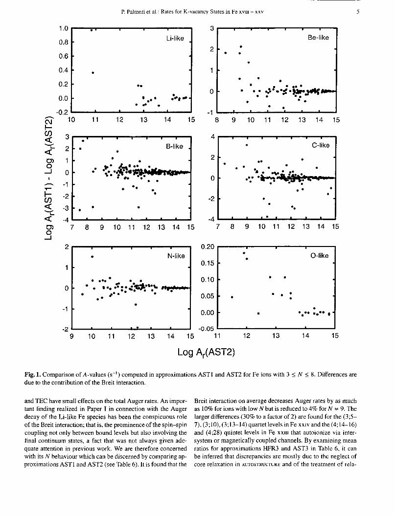
The radiative rates, A,(k, i), and total radiative widths, A,@) = 2, A,(k, i), computed with approximation AST3 are listed in Tables 1-2. In order to estimate their accuracy, we have con- sidered several effects that were found relevant in Paper I: CI, Breit interaction, fine tuning, and variations along the isonu- clear sequence. It is found that CI from configurations with 11 = 3 orbitals is of little importance and can be practically ne- glected. The contributions of the Breit interaction are brought out by comparing A-values computed with approximations
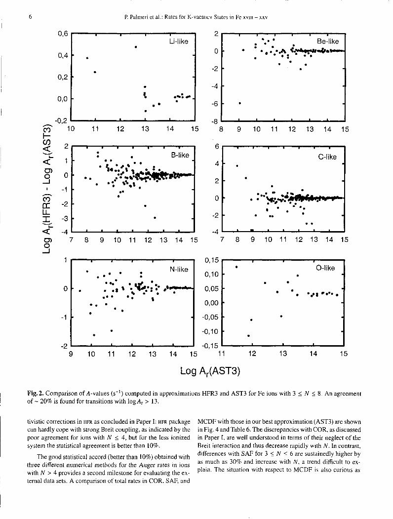
ASTl and AST2 as shown in Fig. 1 for species with 3 < N 5 8. The general trend is that differences become more conspic- uous for the weaker transitions, from - 10% for those with log A, > 14 to several orders of magnitude for the smaller rates. This trend is broken for 3 notorious transitions with log A, > 13 in the C-like system: (6;29,3-4) and (6;26,4). The upper energy levels of these transitions belong to the strongly mixed ‘Do and 3P0 terms of ls2s22p3 discussed in the previous section. In this instance, the spin-spin coupling causes drastic changes. If they are discarded, the average ratios for transitions with logA, > 13 listed in Table 3 for the ASTl/AST2 data sets in- dicate that this effect is of the order of - 15% and does not seem to decrease with N . Changes originating from fine tun- ing (TEC)-see R(AST2, AST3) in Table 34 i sp lay a similar behavior and are not larger (less than 17%) if a few sensitive transitions are put aside, namely (4;20,4), (6;26,34), (6;28,2) and (6;29,4). Moreover, the key comparison in this respect is between AST3 and HFR3 for many reasons; they are two in- dependent numerical methods which have been used to gen- erate complete sets of A-values; their fine tuning capabilities follow different approaches, AUTOSTRUCTURE employs TEC (see Section 2.1) whereas HFR relies on the treatment of radial in- tegrals as fitting parameters; and their respective weaknesses have been well established in Paper I, the former by adopting an orthogonal orbital basis which excludes core relaxation ef- fects and the latter with a reduced implementation of the Breit interaction. It is shown in Fig. 2 and Table 3 that for log A, > 13 AST3 and HFR3 lead to A-values stable to within 20%, an ac- ceptable level of accuracy mainly limited by code options. This result certainly establishes a milestone for evaluating previous work. A-values in COR and SAF agree with those in AST3 to - 20% (see Fig. 3 and Table 3) if a handful of transitions with discrepancies larger than a factor of 2 are excluded: (6;23,4), (6;26,4) and (6;29,4) in COR and those listed in Table 4 in SAF. On the other hand, it may be seen in Fig. 3 that the number of transitions in MCDF displaying large discrepancies with AST3 is noticeably larger. These transitions are listed in Table 5 and were excluded from the statistical indicators of Table 3. A con- trasting and worrying aspect is that while the mean ratios for N I 5 are within a comparable accuracy interval (- 17%), that for the C-like ion indicates A-values that are on average 20% higher with a scatter of the order of 30%. This finding seems to point out at numerical problems in the MCDF radiative data for Fe xxr.
6. Auger decay data
Total Auger rates computed in approximation AST3 for the K- vacancy levels of the n = 2 complex in Fe xxrv-Fe xvm are presented in Table 1. It can be seen that while levels in ions with N > 4 have Auger widths of logA,(i) > 14, with the sole exception of the sextet (5; 19), levels in the Li- and Be-like systems have widths as low as IO9 s-’ making them more sus- ceptible to the approximation level. This assertion is supported by the mean ratios R(BPR1, ASTI) for 3 6 N _< 9 given in Table 6 where standard deviations of 14% and 1 1 % for Fe XXIV
and Fe XXIII, respectively, decrease to - 5% in species with N > 4. It is found that extra-complex configuration interaction
P. Palmeri et al.: Rates for K-vacancy States in Fe XVIII - xxv 5
a <?
W
1 .o
0.8
0.6
0.4
0.2
0.0
-0.2
B-like . 2-• .
.
1 -
0 -
-1
-2
-3
11 12 13 14 15 n cv l o I-
- - .
0) 0 -I
I
n
F a cn W
. .
aL -4 1..1)1111 0) 0 1
7 8 9 10 11 12 13 14 15
2 1 I 1 1 I I i
1
0
. N-like
-2 - l t . , . : . I 1 9 10 11 12 13 14 15
3r I 1 1 I I 1 I
8 9 10 11 12 13 14 15
' 4 I 1 1 1 1 1 1 . C-like
. 0.
I I I . I I I I I 7 8 9 10 11 12 13 14 15
0.20
0.15
0.10
0.05
0.00
-0.05 11 12 13 14 15
Log A,(AST2)
Fig. 1. Comparison of A-values (s-') computed in approximations ASTl and AST2 for Fe ions with 3 5 N 5 8. Differences are due to the contribution of the Breit interaction.
and TEC have small effects on the total Auger rates. An impor- tant finding realized in Paper I in connection with the Auger decay of the Li-like Fe species has been the conspicuous role of the Breit interaction; that is, the prominence of the spin-spin coupling not only between bound levels but also involving the final continuum states, a fact that was not always given ade- quate attention in previous work. We are therefore concerned with its N behaviour which can be discerned by comparing ap- proximations ASTl and AST2 (see Table 6). It is found that the
Breit interaction on average decreases Auger rates by as much as 10% for ions with low N but is reduced to 4% for N = 9. The larger differences (30% to a factor of 2) are found for the (3;5- 7), (3;10), (3;13-14) quartet levels in Fe XXIV and the (4;14-16) and (4;28) quintet levels in Fe XXIII that autoionize via inter- system or magnetically coupled channels. By examining mean ratios for approximations HFR3 and AST3 in Table 6, i t can be inferred that discrepancies are mostly due to the neglect of core relaxation in AUTOSTRUCTURE and of the treatment of rela-
6
Li-l i ke . P. Palmeri et al.: Rates for K-vacancv States in Fe XVIII - xxv
v
aL 1 -
2 O D -J
m CT -2 LL I -3
eL -4
' -1 - v
I I I I I I I . . . 6-like e . -
0 .
- 0.
- . . - .
I I I I I I I I
4 -
2 -
0 '
-2
I I I I I
-
N-like
e . * .
-1 I * I * .
-2 ' I a I I I
I I I I I I 1
-2 t . .
8 9 10 11 12 13 14 15
6 1 m 8 8 I I I I 1
. . 1 C-like
. e
-4 . I I . I . I 7 8 9 10 11 12 13 14 15
0,15
0 , l O
0,05
0,oo
-0, -0'05 t o 3 -0.15 -
9 10 11 12 13 14 15 11 12 13 14 15
Log A,(AST3)
I Fig.2. Comparison of A-values (s-l) computed in approximations HFR3 and AST3 for Fe ions with 3 5 N 5 8. An agreement of - 20% is found for transitions with logA, > 13.
tivistic corrections in HFR as concluded in Paper I: HFR package can hardly cope with strong Breit coupling, as indicated by the poor agreement for ions with N 5 4, but for the less ionized system the statistical agreement is better than 10%.
The good statistical accord (better than 10%) obtained with three different numerical methods for the Auger rates in ions with N > 4 provides a second milestone for evaluating the ex- ternal data sets. A comparison of total rates in COR, SAF, and
MCDF with those in our best approximation (AST3) are shown in Fig. 4 and Table 6 . The discrepancies with COR, as discussed in Paper I, are well understood in terms of their neglect of the Breit interaction and thus decrease rapidly with N . In contrast, differences with SAF for 3 5 N I 6 are sustainedly higher by as much as 30% and increase with N , a trend difficult to ex- plain. The situation with respect to MCDF i:, also curious as
I
1.0
Be-like 0.5 - VV
T V
T T
-1 .o
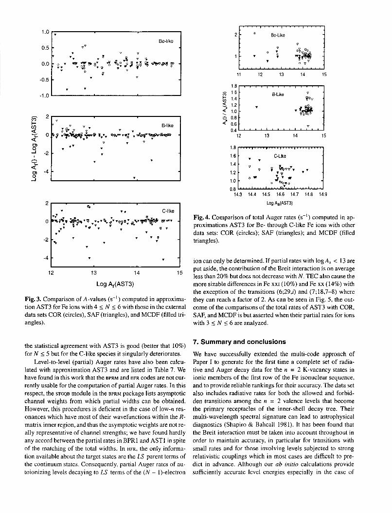
67 21 v 1
Fig. 3. Comparison of A-values (s-l) computed in approxima- tion AST3 for Fe ions with 4 I N I 6 with those in the external data sets COR (circles), SAF (triangles), and MCDF (filled tri- angles).
the statistical agreement with AST3 is good (better that 10%) for N I 5 but for the C-like species it singularly deteriorates.
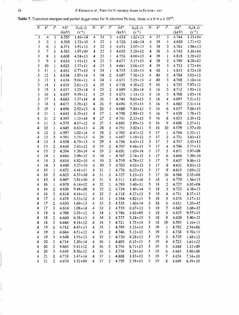
Level-to-level (partial) Auger rates have also been calcu- lated with approximation AST3 and are listed in Table 7. We have found in this work that the BPRM and HFR codes are not cur- rently usable for the computation of partial Auger rates. In this respect, the STGQB module in the BPRM package lists asymptotic channel weights from which partial widths can be obtained. However, this procedures is deficient in the case of low-n res- onances which have most of their wavefunctions within the R- matrix inner region, and thus the asymptotic weights are not re- ally representative of channel strengths; we have found hardly any accord between the partial rates i n BPRl and ASTl in spite of the matching of the total widths. In HFR, the only informa- tion available about the target states are the LS parent terms of the continuum states. Consequently, partial Auger rates of au- toionizing levels decaying to LS terms of the ( N - 1)-electron
0 . . , . , . . . . 0 Be-Like
11 12 13 14 15
li/ 1 .o , 0.8
V B-Like 8’oV
0.6 V
0.4 ” I ’ “ ” ” ”
12 13 14 15
14.3 14.4 14.5 14.6 14.7 14.8 14.9
Log Aa(AST3)
Fig. 4. Comparison of total Auger rates (s-l) computed in ap- proximations AST3 for Be- through C-like Fe ions with other data sets: COR (circles); S A F (triangles); and MCDF (filled triangles).
ion can only be determined. if partial rates with log A, < 13 are put aside, the contribution of the Breit interaction is on average less than 20% but does not decrease with N . TEC also cause the more sizable differences in Fe XXI (10%) and Fe xx (14%) with the exception of the transitions (6;29,i) and (7;18,7-8) where they can reach a factor of 2. As can be seen in Fig. 5 , the out- come of the comparisons of the total rates of AST3 with COR, SAF, and MCDF is but asserted when their partial rates for ions with 3 2 N 5 6 are analyzed.
7. Summary and conclusions
We have successfully extended the multi-code approach of Paper I to generate for the first time a complete set of radia- tive and Auger decay data for the n = 2 K-vacancy states in ionic members of the first row of the Fe isonuclear sequence, and to provide reliable rankings for their accuracy. The data set also includes radiative rates for both the allowed and forbid- den transitions among the n = 2 valence levels that become the primary receptacles of the inner-shell decay tree. Their multi-wavelength spectral signature can lead to astrophysical diagnostics (Shapiro & Bahcall 1981). It has been found that the Breit interaction must be taken into account throughout in order to maintain accuracy, in particular for transitions with small rates and for those involving levels subjected to strong relativistic couplings which in most cases are difficult to pre- dict in advance. Although our ab initio calculations provide sufficiently accurate level energies especially in the case of

VI11 - xxv
2 I '
1 1 B-Like
V v i 0 W y B 0
-1
-2
2 I '
13 14 15
C-Like 1 -
. T V
-1 1 . v
-2 I ,
13 14 15 Log A,(AST3)
Fig.5. Comparison of partial Auger rates (s-l) computed in ap- proximations AST3 for B- through C-like Fe ions with other data sets: COR (circles); SAF (triangles); and MCDF (filled triangles).
HFR, the semi-empirical corrections have been useful to im- prove further the accuracy of our data. In this respect, i t would have been resourceful to have had more reliable estimates of the strongly coupled and tricky levels of the ls2s22p3 con- figuration in Fe XXI and of the questionable solar identifica- tions of the ls2s22p4 2 L ~ and ls2s22p6 2S~/z components in Fe xx and Fe XVIII, respectively, which required revised esti- mates with the laboratory wavelengths of Beiersdorfer et al. (1993) and Decaux et al. (1997) in EXP2. The latter has not been an easy task since, in spite of the quoted high accuracy, their wavelength data lack the structural consistency that war- rants a unique set of spectroscopic level energies. By exten- sive comparisons with results from the approximations consid- ered, previous calculations and experiment, the statistical ac- curacy of present level-energy data set has been established at better than 3 eV. Our wavelengths and Auger-electron kinetic energies have been derived from the experimental levels when available otherwise from the theoretical values which ensures in the case of the former a statistical accuracy close to +2 mA.
With respect to the A-values and partial Auger rates, i t has been found that very little can be asserted about transitions with values under loi3 s-'. The accuracy otherwise has been
firmly ranked by means of comparisons of several data sets at 20%. Relativistic effects are particularly conspicuous in Fe ions with N 2 4, but become more manageable for the less ionized species. We are therefore puzzled with the large systematic dis- crepancies encountered in S A F and MCDF which affect even the large (greater than l O I 4 s-') total widths of the higher N systems which in our view can only be attributed to numerical problems. By contrast the data in COR are in general within the proposed bounds in spite of the neglect of the spin-spin bound-free couplings in the Auger processes.
It has been found that the BPRM and the HFR suites are currently not usable for the calculation of partial Auger rates which are now in demand in the formal modeling of ionization balances and post-Auger radiative emissions. Taking also into consideration their present shortcomings in the representation of the two-body operators of the Breit interaction, our early statement about AUTOSTRUCTURE being the platform of choice for inner-shell studies is reaffirmed. We have already made fast progress in tackling the very interesting features of the decay pathways of members of the second row (10 I N I 17) which will be reported elsewhere.
Acknowledgements. We are grateful to Dr. Margerite Comille, Observatoire de Meudon, France for private communications regardig the approximations made in the COR and SAF data sets. CM acknowl- edges a Senior Research Associateship from the National Research Council. PP acknowledges a Research Associatestup from University of Maryland. MAB acknowledges partial support from FONACIT, Venezuela, Proyecto No. S1-20011000912.
References
Badnell, N. R. 1986, J. Phys. B 19,3827 Badnell, N. R. 1997, J. Phys. B 30, 1 Bautista, M., Mendoza, C., Palmeri, P., Kallman, T. R. 2002, A&A,
Becker, S. R., Butler, K., Zeippen, C. J. 1989, A&A 221, 375 Beiersdorfer, P., Phillips, T., Jacobs, V. L., et al. 1993, ApJ 409. 846 Berrington, K. A., Burke, P. G., Butler, K., et al. 1987, J. Phys. B 20,
Berrington, K. A., Burke, P. G., Chang, J. J., et al. 1974, Comput.
Berrington, K. A., Burke, P. G., Le Doumeuf, M., et al. 1978, Comput.
BiCmont, E., FrCmat, Y., Quinet, P. 1999, At. Data Nucl. Data Tables
Burke, P. G., Hibbert, A., Robb, W.D. 1971,J. Phys. B 4, 153 Burke, P. G., Seaton, M. J. 1971, Meth. Cornp. Phys. IO, 1 Chen M. H. 1986, At. Data Nucl. Data Tables 34,301 Chen M. H., Crasemann, B. 1987, At. Data Nucl. Data Tables 37,419 Chen, M. H., Crasemann, B. 1988, At. Data Nucl. DataTables 38,381 Chen, M. H., Reed, K. J., McWilliams, D. M., et al. 1997, At. Data
Cowan, R. D. 1981, The Theory of Atomic Structure and Spectra
Decaux, V., Beiersdorfer, P., Kahn, S. M., Jacobs, V. L. 1997, ApJ 482,
Drake, G . W. E 1986, Phys. Rev. A34,2871 Dubau, J . , Loulergue, M. 1981, Phys. Scr 23, 136 Eissner, W., Jones, M., Nussbaumer, H. 1974, Comput. Phys.
submitted
6379
Phys. Commun. 8, 149
Phys. Commun. 14,367
71, 117
Nucl. Data Tables 65, 289
(Berkeley, CA: University of California Press)
I076
Commun. 8,270

P. Palmeri et al.: Rates for K-vacancy States in Fe XVII I - xxv
Eissner. W., Nussbaurner, H. 1969, J. Phys. B 2, 1028 Feldrnan, U., Doschek, G . A., Kreplin, R. W. 1980, ApJ 238,365 Galavis, M. E., Mendoza, C., Zeippen, C. J. 1997, A&AS 123, 159 Galavis, M. E., Mendoza, C.,Zeippen, C. J. 1998, A&AS 131,499 Kato, T., Safronova, U. I., Shlyaptseva, A. S., et al. 1997, At. Data
Mendoza, C., Zeippen, C. J., Storey, P. J. 1999, A&AS 135, 159 Quigley, L., Berrington, K. 1996, J. Phys. B 29,4529 Quigley, L., Berrington, K., Pelan, J. 1998, Cornput. Phys. Commun.
Safronova, U. I., Shlyaptseva, A. S. 1996, Phys. Scr 54,254 Safronova, U. I., Shlyaptseva, A. S. 1999, Phys. Scr 60,36 Safronova, U. I., Shlyaptseva, A. S., Comille, M., Dubau, J. 1998,
Safronova, U. I . , Umov, A. M. 1980, J. Phys. B 13, 869 Scott, N. S., Burke, P. G. 1980, J. Phys. B 13,4299 Scott, N. S., Taylor, K. T. 1982, Comput. Phys. Commun. 25,347 Seely, J. F., Feldman, U., Safronova, U. I. 1986, ApJ 304, 838 Shapiro, P. R., Bahcall, J. N. 1981, ApJ 245, 335 Shirai, T., Sugar, J., Musgrove, A., Wiese, W. L. 2000, J. Phys. Chem.
Nucl. Data Tables 67,225
114,225
Phys. Scr 57,395
Ref. Data, Monograph 8
9

10 P. Palmeri et al.: Rates for K-vacancy States in Fe XVIII - xxv
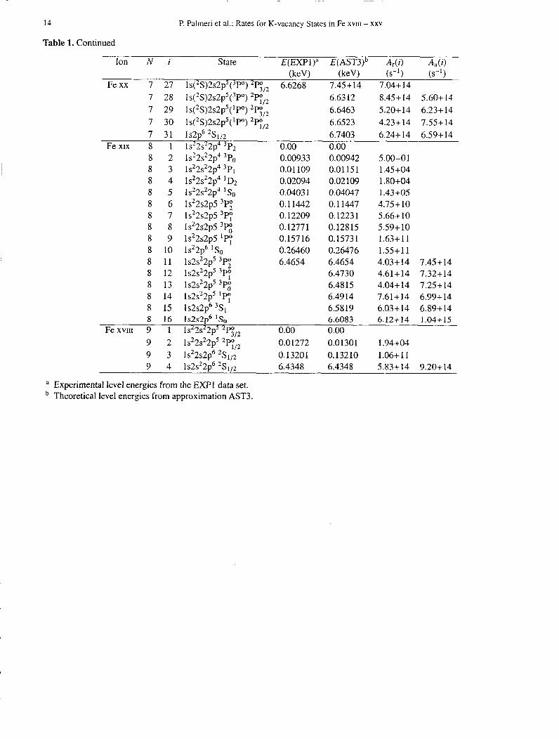
Table 1. Energies and total radiative and Auger widths for levels within the n = 2 complex of N-electron (2 I N I 9) Fe ions. Note: CI * b n x 10”.
Ion N i State E(EXP1)“ E(AST3)b A,( i )
2 2 2 3 2 4 2 5 2 6 2 7
FexxIv 3 1 3 2 3 3 3 4 3 5 3 6 3 7 3 8 3 9 3 10 3 11 3 12 3 13 3 14 3 15 3 16 3 17 3 18
6.6366 6.6655 6.6676 6.6680 6.6823 6.7004 0.00 0.04860 0.0645 7 6.6004 6.6137 6.6 167
6.6535 6.6619 6.6710 6.6764 6.6792 6.6793 6.6850 6.7027 6.7046 6.7090 6.7224
6.6367 6.6656 6.6676 6.6684 6.68 19 6.7005 0.00 0.04778 0.06498 6.6003 6.6131 6.6169 6.6285 6.6525 6.6623 6.6706 6.6764 6.6791 6.6792 6.6850 6.7027 6.7041 6.7089 6.7225
2.08+08 3.74+08 4.35+ 13 4.11+09 7.90+09 4.61 +14
1.77+09 4.30+09 1.88+13 4.97+12 1.55+13 6.36+09 3.01+14 4.7 1+14 2.18+13 1.86+14 4.19+12 1.06+ 13 3.58+ 13 3.50+14 6.9 1+ 14 2.05+14 6.16+14
1.43+ 14 1.33+10 3.91+11 1.97+09 4.24+13 1.41+11 3.37+11 6.77+13 1.07+ 14 9.66+ 1 1 2.61+13 1.25+14 9.39+11 1.37+ 14 3.28+13
3 19 ~ S ( ~ S ) ~ & ’ S ) *S1;2 6.7415 6.7414 2.50+14 2.92+13 Fexxrrr 4 1 ls22s2 ‘SO 0.00 0.00
4 2 4 3 4 4 4 5 4 6 4 7 4 8 4 9 4 10 4 11 4 12 4 13 4 14 4 15 4 16 4 17 4 18 4 19 4 20 4 21 4 22
1 s’2s2p 3 q
1 s22s2p 3P’: 1 s’2s2p 3 5
1 s22s2p ‘P; 1s22p2 3 ~ 0
1s22p2 3 ~ 1
1s22p2 3 ~ 2
1 s22p2 1 so ls222p 3 5
ls2s22p 3 q
1 s2s22p 3P0 I s(2~)2s2p5(4~) 5 ~ 1
I s ( ~ s ) ~ s ~ P ~ ( ~ P ) s ~ 2
ls(2S)2s2p2(4P) 5P3 1 s2s22p IPO ~ s ( ~ s ) ~ s ~ P i ( 4 ~ ) 3 ~ 0
ls(?S)2s2p2(4P) 3P,
1 s22p2 D2
l ~ ( ~ S ) 2 ~ 2 p ~ ( ’ D ) 3D2 1 s(*S)2s2p2(’D) 3D3 l ~ ( ~ S ) 2 ~ 2 p ’ ( ~ D ) 3D1
0.043 17 0.04701 0.05849 0.09 329 0.11854 0.12736 0.13287 0.14930 0.17638
6.5958
6.6287 6.6287 6.6588
6.6643 6.6686 6.6703
0.04273 0.04670 0.05877 0.09329 0.11811 0.12749 0.13281 0.14937 0.17639 6.5938 6.5958 6.6086 6.6148 6.6223 6.6286 6.6287 6.6588 6.6629 6.6648 6.6685 6.6695
5.0 1 +07 1.05+04 1.95+ 10 1.23+10 1.5 1+10 1.3 1+10 9.75+09 3.15+10 8.04+12 4.06+ 13 1.04+ 1 3 1.17+13 5.06+ 12 1.02+ 13 4.53+14 6.01+ 14 5.51+14 3.36+14 2.23+14 3.40+14
1.83+ 14 1.86+14 1.91+14 2.22+12 5.25+11 6.55+12 1.28+14 7.13+ 13 6.86+ 13 1.34+ 14 1.63+14 1.30+14

P. Palrneri et al.: Rates for K-vacancy States in Fe X V I H - xxv
Table 1. Continued
11
Ion N i State E(EXP1)a E(AST3)b A,(i) M i ) (keV) (keW (s-') (s-')
Fe xxni 4 23 ~ s ( ~ S ) ~ S ~ P ' ( ~ P ) 3P2 6.6762 5.19+14 9.44+13 4 24 ~ s ( ~ S ) ~ S ~ & ~ S ) 3 S ~ 4 25 ~ s ( ~ s ) ~ s ~ P ~ ( ~ P ) 'pO 4 26 l ~ ( ~ S ) 2 ~ 2 p ~ ( ~ D ) 'D2 4 27 I S ( ~ S ) ~ S ~ P ~ ( ~ P ) 3 ~ 1
4 29 I S ( ~ S ) ~ S ~ P ~ ( ~ P ) 3 ~ 2
4 28 1 ~ 2 ~ ~ js;
4 30 l ~ ( ~ S ) 2 ~ 2 p ~ ( ~ P ) 'Pi 4 31 l ~ ( ~ S ) 2 ~ 2 p ~ ( ~ S ) 'So 4 32 ls2p3 3Dy 4 33 ls2p3 3D; 4 34 ls2p3 3D9
4 36 ls2p3 'Di 4 35 is2p3 3sy
4 37 1 ~ 2 ~ ~ 3q 4 38 1 ~ 2 ~ ~ 3~
4 39 is2p3 3e
6.6858 6.6857 6.6883
6.6947 6.6947 6.7005 6.7016 6.7065
6.7177 6.7177 6.7264 6.7264
6.7330 6.7344 6.7363 6.7450 6.7535 6.7586 6.7605 6.768 1
1.62+ 14 1.30+14 2.62+ 14 1.63+ 14 1.18+13 5.99+13 6.67+14 2.23+14 3.08+14 2.35+14 2.32+14 7.98+14 5.20+14 2.27+14 3.20+14 3.96+14
I .29+ 14 1.38+14 2.28+14 1.11+14 5.95+12 2.14+14 5.57+13 2.18+14 1.92+14 2.07+14 2.28+14 4.80+13 1.97+14 1.41 + 14 1.37+14 1.77+14
6.7834 6.83+14 1.31+14
5 2 5 3 5 4 5 5 5 6 5 7 5 8 5 9 5 10 5 11 5 12 5 13 5 14 5 15 5 16 5 17 5 18 5 19 5 20 5 21 5 22 5 23 5 24 5 25 5 26 5 27 5 28 5 29 5 30
lS2S22p2 4P5/2 ls(2S)2s2p3(5SO) 6sgI2
ls2s22p2 2P'/2 ls2s22p2 2D3/2 ls2s22p2 2D5/2 1s2s22p2 2 ~ 3 / 2
1 s2s22p2 2s, /2
l~ (~S)2s2p~(~DO) 4D0 312
1 s( 2S)2s2p3 ( 3Do) 4D&2 1 s( 2S)2s2p3 ( 3Do) 4Dy12 l ~ ( ~ S ) 2 s 2 p ~ ( ~ D ' ) 4D;12 ls(2S)2s2p3(5SO) 4s;/,
lsPS)2s2d(3P) 4PP,, L , i . . . . .
0.00 0.00 0.01466 0.05016 0.05706 0.06364 0.09 129 0.094 13 0.105 84 0.12 130 0.12303 0.15569 0.17310 0.17687 0.19461 0.201 8 1
6.5863 6.5865 6.59 17 6.6012 6.61 17
0.0 1526 0.05006 0.05741 0.06423 0.09147 0.09467 0.10566 0.12173 0.12370 0.15608 0.17334 0.17737 0.19458 0.20243 6.5540 6.5626 6.5682 6.5801 6.5846 6.5868 6.5922 6.6027 6.6121 6.6294 6.6305 6.63 17 6.6328 6.6366 6.6501
1.49+04 9.93+07 1.04+07 7.23+07 1.09+10 6.03+09 3.84+ 10 3.69+10 5.06+10 4.52+ 10 2.20+10 2.11+10 4.44+10 4.39+10 3.15+13 2.38+14 1.26+13 2.32+14 2.72+13 2.50+14 6.11+12 4.21+12 6.31+14 1.58+14 3.67+14 2.87+14 2.07+14 3.41+14 5.46+14 1.98+14 2.76+14 2.82+14 3.29+14 1.92+14 2.25+14 2.20+14 2.38+14 2.27+14 2.23+14 2.35+14 7.42+14 1.04+14 2.30+14 1.78+14

12 P. Palmeri et al.: Rates for K-vacancy States in Fe X V I I I - xxv
Table 1. Continued
Ion N i State E(EXP1)2 E(AST3)b A , ( i ) &(i) (keV) (keV) (s-') (s-l)
Fe XXII 5 3 1 I s ( ~ S ) ~ S ~ ~ ~ ( ~ P O ) 4Pz/2 6.6508 2.59+14 1.88+14 5 32 l ~ ( ~ S ) 2 ~ 2 p ~ ( ~ P ~ ) 4P;/2 6.6509 2.52+14 1.93+14 5 33 l ~ ( ~ S ) 2 ~ 2 p ~ ( ~ D ' ) 'DY12 6.6660 4.83+14 3.48+14 5 34 l~ (~S)2s2p~(~DO) 2Do 6.6712 5.84+14 3.32+14 5 35 ls(2S)2s2p3(3SO) 4s;/, 6.6749 1.49+14 2.29+14 5 36 l~(~S)2s2p'('DO) 2Do 6.6807 5.27+14 2.78+14 5 37 ls('S)2s2p3(3P") *P?/, 6.6825 6.66+14 2.35+14 5 38 l~(~S)2s2p~('DO) 2Do 6.6871 2.93+14 3.69+14 5 39 ls('S)2s2p3(3PO) 2p;/, 6.6949 4.75+14 2.81+14 5 40 l ~ ( ~ S ) 2 ~ 2 p ~ ( ' P ' ) 2q/2 6.6966 4.50+14 2.78+14 5 41 l ~ ( ~ S ) 2 ~ 2 p ~ ( ' P ~ ) 2P;/2 6.7069 2.32+14 3.55+14 5 42 l ~ ( ~ S ) 2 ~ 2 p ~ ( ~ S ~ ) 2 S y / 2 6.7121 6.99+14 1.48+14 5 43 i s2p44~512 6.7227 2.30+14 2.56+14 5 44 1s2p44~3 /2 6.7330 2.52+ 14 2.50+14 5 45 is2p4 4 ~ 1 1 2 6.7363 2.35+14 2.49+14 5 46 6.7505 6.00+14 3.22+14 5 47 ls2p4 2D5/2 6.7546 4.34+14 3.86+14 5 48 ls2p4 2P3/2 6.7627 7.22+14 2.99+14 5 49 i s 2 p 4 2 ~ 1 / 2 6.7634 8.36+14 2.51+14 5 50 1 ~ 2 p ~ ~ s ~ / ~ 6.7893 5.00+14 2.70+14
512
312
512
FexxI 6 1 1 ~ ~ 2 ~ ~ 2 ~ ~ 3 P ~ 0.00 0.00 6 2 6 3 6 4 6 5 6 6 6 7 6 8 6 9 6 10 6 11 6 12 6 13 6 14 6 15 6 16 6 17 6 18 6 19 6 20 6 21 6 22 6 23 6 24 6 25 6 26 6 27 6 28
ls22s22p2 3PI
is22s22p2 3 ~ 2
ls22s22p2 'so 1 s22s2p3 5s;
ls22s22p2 'D2
ls22s2p3 3D: ls22s2p3 'D; ls22s2p3 3Di ls22s2p3 'Po" 1 s22s2p3 3Py ls22s2p3 3 q
ls22s2p3 3s:
ls22s2p3 1P; ls22s2p3 'D4
iS22p4 3 ~ 2
is22p4 3 ~ 0
1 s22p4 3 ~ 1
1 s22p4 so ls22p4 'D2
ls2s22p3 5s; ls2s22p3 3Dy ls2s22p3 3D4 ls2s22p3 3DY
ls2s22p3 ID; ls2s22p3 3.57
ls2s'2p3 3P7 is2s22p3 3q
0.00916 0.01455 0.03032 0.04612 0.06037 0.09630 0.09638 0.09963 0.1 1361 0.11468 0.11685 0.13585 0.13976 0.15636 0.20412 0.21520 0.2 1579 0.22529 0.25394
6.5436 6.545 1 6.55 17 6.5550 6.5621
0.009 68 0.01496 0.03073 0.04653 0.0607 8 0.09648 0.09666 0.10022 0.1 1380 0.11502 0.11733 0.13624 0.14017 0.15677 0.20429 0.21562 0.21658 0.22570 0.25435 6.5 182 6.5443 6.5467 6.5499 6.5550 6.5619 6.5642 6.5659
6.54+03 8.39+02 3.19+04 1.39+05 7.05+07 1.30+ 10 9.62 + 09 7.39+09 2.28+10 2.42+10 2.17+10 9.93+10 5.45+ 10 9.07 + 1 0 6.26+10 7.28+10 7.32+10 4.80+10 8.82+10 1.48+13 3.63+14 2.30+14 2.17+14
4.90+14 2.25+ 14 3.18+14
.6.88+14
2.82+14 3.95+14 4.38+14 4.58+14 2.41 +I4 3.97+14 4.08+14 4.07+14

~ ~~ ~- ~
P Palrneri et ai.: Rates for K-vacancy States in Fe xviii - xxv
Table 1. Continued
Ion N i State E(EXPl)a E(AST3)b A,(i) Aa(i) (keV) (keV) (s- ) (s-')
Fexxi 6 29 ls2sL2p' 'P: 6.5757 6.5741 3.69+14 4.18+14 6 30 6 31 6 32 6 33 6 34 6 35 6 36 6 37 6 38 6 39 6 40 6 41 6 42 6 43 6 44 6 45 6 46 6 47 6 48 6 49 6 50
6.5841 6.5841 6.5877 6.5970 6.6009 6.6316 6.6349 6.6377 6.6394 6.6429 6.6437 6.6590 6.6605 6.6696 6.6696 6.6727 6.6868 6.6947 6.7355 6.7435 6.7524 6.7629
6.36+ 14 3.46+14 2.20+14 2.67+14 2.24+14 2.60+14 2.24+14 2.63+14 7.44+14 3.81+14 5.95+14 3.76+14 4.29+14 4.13+14 4.90+14 4.34+14 6.81+14 3.71+14 8.35+14 3.78+14 4.26+14 3.82+14 3.78+14 4.93+14 3.20+14 4.73+14 3.53+14 6.14+14 3.57+14 4.25+14 7.88+14 3.19+14 3.91+14 5.74+14 4.26+14 4.70+14 4.88+14 4.66+14 4.28+14 4.58+14 8.12+ 14 4.67+ 14
I
Fexx 7 1 ls22s22p3 4S:,, 0.00 0.00 7 2 ls22s22p32D-& 0.01719 7 3 ls22s22p3 2D:12 0.02184 7 4 is22s22p3 2q12 0.03227 7 5 ls22s22p3 2 q 1 2 0.04009 7 6 7 7 7 8 7 9 7 10 7 11 7 12 7 13 7 14 7 15 7 16 7 17 7 18 7 19 7 20 7 21 7 22 7 23 7 24 7 25 7 26
0.09333 0.10175 0.10445 0.12926 0.13 122 0.148 19 0.15404 0.16614 0.24230 0.25565 6.4966 6.5060 6.508 1 6.5237 6.5283 6.5335 6.5345 6.5497
0.01705 0.02 194 0.03195 0.04026 0.093 17 0.10190 0.10464 0.12913 0.13 132 0.148 19 0.15386 0.16653 0.242 13 0.25602 6.4964 6.5063 6.5082 6.5236 6.5283 6.5324 6.5353 6.5496 6.5899 6.5974 6.6039
1.49+04 1.87+03 3.69+04 8.30+04 1.34+ 10 1.79+ 10 2.02 + 1 0 4.50+10 3.64+10 8.28+10 1.33+11 1.24+11 9.96+ 10 1.09+11 2.19+14 5.38+14 2.39+14 5.26+14 2.36+14 5.31+14 5.98+14 5.62+14 4.10+14 6.25+14 6.89+14 4.83+14 6.48+ 14 4.94+ 14 5.71+14 5.33+14 4.19+14 4.94+14 4.31+14 4.92+14 4.28+14 4.85+14
13
14 P. Palmeri et al.: Rates for K-vacancy States in Fe XVIII - xxv
Table 1. Continued
Ion N i State E(EXP1)" E(AST3)b A,(i) &(i) (keV) (keV) 6-1) (s-')
Fe xx 7 27 l ~ ( ~ S ) 2 s 2 p ~ ( ~ P ~ ) 'qI2 6.6268 7.45+14 7.04+14 7 28 ls('S)2~2p~(~PO) 2p1)12 6.63 12 8.45+14 5.60+14 7 29 l~(~S)2s2p~('PO) 2P;12 6.6463 5.20+14 6.23+14 7 30 ls('S)2s2p5('P") 2Pp/2 6.6523 4.23+14 7.55+14 7 31 ls2p6 2S1/2 6.7403 6.24+14 6.59+14
Fexrx 8 1 ls'2s22p4 3P2 0.00 0.00 8 2 ls'2s22p4 3Po
8 4 ls22s22p4 'Dz 8 5 ls22s22p4 'So
8 3 ls22s22p4 3P1
8 6 s22s2p5 3Py 8 7 s22s2p5 3Py 8 8 s22s2p5 3Pg 8 9 s22s2p5 'Pp
8 11 ls2s22p5 3P; 8 12 ls2s22p5 'P; 8 13 ls2s22p5 3P: 8 14 ls2s22p5 'Pp 8 15 ls2s2p6 3S1 8 16 1 . ~ 2 ~ 2 ~ ~ 'SO
8 10 s22p6 'So
0.00933 0.01 109 0.02094 0.0403 1 0.1 1442 0.12209 0.12771 0.15716 0.2 6460 6.4654
0.00942 0.01 15 1 0.02109 0.04047 0.1 1447 0.1223 1 0.12815 0.1573 1 0.26476 6.4654 6.4730 6.48 15 6.4914 6.5819 6.6083
5.00-01 1.45+04 1.80+04 1.43+05 4.75+10 5.66+10 5.59+10 1.63+11 1.55+11 4.03+14 7.45+14 4.61+14 7.32+14 4.04+14 7.25+14 7.61+14 6.99+14 6.03+14 6.89+14 6.12+14 1.04+15 . . .
Fexvrr~ 9 1 ls22s22p5 2q12 0.00 0.00 9 2 ls22s22ps2P(1/2 0.01272 0.01301 1.94+04 9 3 lS22S2P62S,/2 0.13201 0.13210 1.06+11 9 4 ls2s22p62s',2 6.4348 6.4348 5.83+14 9.20+14
a Experimental level energies from the Em1 data set. Theoretical level energies from approximation AST3.

P. Palmer1 et al.: Rates for K-vacancy States in Fe X V I I I - xxv 15
Table 2. Wavelengths and radiative rates for N-electron Fe ions. Note: a f 6 = a x loib.
N k i A A,(k,i) N k i R A,(k,i) N k i R A S k , i)
2 1 1.8682 2.08+08 4 166.69 7.44+09 4 24 2 1.8665 5.27+12 (A) k-') (A) (s-') (A) (s-')
L
2 2 2 2 2 2 2 2 2 3 3 3 3 3 3 3 3 3 3 3 3 3 3 3 3 3 3 3 3 3 3 3 3 3 3 3 4 4 4 4 4 4 4 4 4 4
3 2 4 1 4 2 5 1 6 1 6 2 7 1 7 2 7 5 2 1 3 1 3 2 4 2 4 3 5 1 6 1 7 1 7 3 8 1 9 1
10 2 10 3 11 1 12 1 13 2 13 3 14 3 15 2 15 3 16 2 16 3 17 3 18 2 18 3 19 2 19 3 3 1 4 1 4 3 5 1 6 3 6 5 7 2 7 3 7 4 7 5
428.23 1.8595 400.30
1.8554 271.12 1.8504 194.28 382.76 255.1 1 192.03 776.55 1.8924 1.8970 1.8747 1.8738 1 .8706b 1 .8890b 1.8635 1.861 1 1.8722 1.8767 1.8570 1.8563 1.8699 1.8744 1.8728 1.8633 1.8678 1.8628 1.8672 1.8660 1.8578 1.8622 1.8525 1.8569 263.77 211.96 1079.3 132.91 173.32 490.94 147.27 154.30 180.04 363.91
3.74+08 4.35+13 4.12+08 4.1 1 +09a 6.48+09 1.42+09 4.61+14 3.40+08 4.69+08 1.77+09 4.30+09 2.08+04 9.27+ 12 9.52+12 4.97+ 12 1.5S+ 13 6.16+09 1.94+08 3.01+14 4.7 1+14 2.17+ 13 9.12+ 10 1.86+14 4.19+12 4.51+10 1.06+ 13 3.58+13 3.14+14 3.64+13 5.3 1+ 14 1.60+14 2.05+ 14 9.69+12 6.07+ 14 I .03+ 13 2.40+14 5.01+07 7.71+00 1.05+04 1.95+10 1.22+10 2.26+07 6.52+09 4.13+09 4.42 + 09 8.10+06
4 8 3 144.39 5.31+09
4 8 4 8 4 9 4 9 4 9 4 10 4 10 4 11 4 12 4 12 4 12 4 12 4 12 4 12 4 13 4 13 4 13 4 14 4 14 4 14 4 14 4 15 4 15 4 15 4 16 4 17 4 17 4 17 4 17 4 17 4 17 4 18 4 18 4 19 4 19 4 19 4 19 4 20 4 20 4 20 4 21 4 22 4 22 4 22 4 22 4 23 4 23 4 23
5 3 4 5 3 5 7 1 6 7 8 9
10 7 8 9 2 3 4 5 3 4 5 4 1 6 7 8 9
10 3 5 2 3 4 5 3 4 5 4 2 3 4 5 3 4
313.19 121.20 136.53 22 1.34 95.834 149.21 1.9174b 1.8797 1.9141 1.9167 1.9184 1.9233 1.9314 1.91 30b 1.9146b 1.9 1 9 5 ~ ~ 1.8867b 1.8878b 1.8911b 1.9012b 1.8856b 1 .8889b 1 .8990b 1.8871 1.8704 1.9045 1.907 1 1.9087 1.9135 1.9215 1.8752 1.8884 1.8730b 1.8741b 1.8773b 1.8873b 1.8736 1.8769 1.8868 1.8757 1.8708 1.8719 1.8752 1.885 1 1 .8703b 1.8735b
3.74+08 4.74+08 4.81+09 4.47+09 1.72+08 3.14+10 8.04+12 3.13+13 3.69+12 2.05+12 3.51+12 3.26+10 8.09+09 3.25+12 5.71+12 1.40+ 12 3.77+12 7.64+12 2.88+ 11 1.12+09 8.10+09 5.05+12 1.65+09 1.02+ 1 3 4.37+14 6.04+ 10 3.47+ 1 1 3.95+12 1.14+13 8.82+11 6.01+14 5.64+11 3.80+14 5.62+13 1.14+14 9.97+10 3.14+14 1.59+13 5.75+12 2.23+14 3.07+12 2.61+14 7.30+13 3.23+ 12 3.47+13 4.70+14
4 24 4 24 4 24 4 25 4 25 4 26 4 26 4 26 4 27 4 27 4 27 4 27 4 28 4 28 4 28 4 29 4 29 4 29 4 30 4 30 4 30 4 30 4 31 4 31 4 32 4 32 4 32 4 32 4 32 4 32 4 33 4 33 4 33 4 34 4 34 4 35 4 35 4 35 4 35 4 35 4 35 4 36 4 36 4 36 4 37 4 38
3 4 5 3 5 3 4 5 2 3 4 5 7 8 9 3 4 5 2 3 4 5 3 5 1 6 7 8 9
10 7 8 9 8 9 1 6 7 8 9
10 7 8 9 7 1
1.8676 1.8708 1.8807 1 .8669b l.88OOb 1.865 1 1.8683 1.8781 1 .8624b 1 .8635b 1.8667b 1.8765b 1.8859b 1.8875b 1 .8922b 1.86 1 8b 1 .8650b 1.8748b 1.8576 1.8586 1.8618 1.8716 1.8562 1.8692 1.8414b 1.8745b 1 .8770b 1.8785b 1.8832b 1.89 1 Ob 1 .8766b 1.8781b 1.8828b 1.8776b 1.8823b 1.8382b 1.8711b 1.8736b 1.875 lb 1 .879Sb 1.8875b 1.8712b 1 .8727b 1 .8774b 1.8697b 1.8340b
3.99+ 13 9.55+ 13 2.18+13 1.00+14 2.97+13 1.96+11 9.67+13 1.65+14 2.73+ 11 8.69+10 1.51+14 1.17+13 6.20+12 5.35+ 12 2.50+11 8.07+ 1 1 5.99+12 5.31+13 1.02+12 8.3 1 +09 1.71+12 6.64+ 14 4.31+10 2.23+14 1.29+1 I 2.57+ 14 2.28+12 4.76+13 1.07+12 2.89+10 2.15+14 2.11+10 2.01 + I3 1.65+14 6.69+13 1.76+10 4.99+13 4.54+14 2.41+14 5.27+13 7.56+10 5.71+11 3.60+14 1.60+ 14 2.27+14 3.42+10
5 1.8834b 1.49+13 4 38 6 1.8667b 2.77+12

16 P. Palmeri et al.: Rates for K-vacancy States in Fe XVIJI - xxv
Table 2. Continued
N k i R A , ( k , i ) N k i R A r ( k , i ) N k i R A r ( k 0
4 38 7 1.8692b 1.19+13 5 13 10 230.28 3.27+09' 5 21 13 1.9343 4.11+12 (A) (s-') (A, (s-') (A> (s-')
4 38 4 38 4 38 4 39 4 39 4 39 4 40 4 40 4 40 4 40 4 40 4 40 5 2 5 3 5 3 5 4 5 4 5 5 5 6 5 6 5 7 5 8 5 8 5 9 5 9 5 10 5 10 5 11 5 11 5 11 5 11 5 11 5 11 5 11 5 11 5 12 5 12 5 12 5 12 5 12 5 12 5 12 5 12 5 13 5 13 5 13
8 9
10 7 8 9 1 6 7 8 9
10 1 1 2 1 2 2 1 2 2 1 2 1 2 1 2 3 4 5 6 7 8 9
10 3 4 5 6 7 8 9
10 4 5 6
1 .8708b 1.8754b l.8831b 1 .8670b 1 .8686b 1.8732b 1.8278b 1 .8603b 1 .8627b 1 .8643b 1.8689b 1 .8766b 845.55 247.19 349.30 217.30 292.46 253.17 135.81 161.80 156.02 117.14 135.98 102.21 116.27 100.77 114.41 117.49 125.71 134.69 192.53 201.41 248.73 360.56 379.68 100.85 106.85 113.27 15 1.56 157.01 184.35 239.37 247.65 103.48 109.49 144.87
2.59+ 14 1.55+13 3.01+13 7.40+12 I . 19+ 12 3.88+14 3.91+11 1.88+11 1.70+12 8.25+ 12 3.85+14 2.87+14 1 .49+04' 8.50+07' 1.44+07' 2.10+06' 8.35+06' 7.23+07c 1.08+ 10' 3.22+07' 6.03+09' 3.84+ 10' 2.60+07' 2.5 8+09' 3.43+ 10' 6.27+09' 4.44+ 10' 1.02+ 10' 1.5 1 + 1 0' 1.96+1OC 1.42+08' 1.34+07' 1.24+08' 1.21+07' 3 .07+07' 4.57+07' 2.22+09' 2.25+08' 7.49+09' 4.88+09' 6.31+09' 7.93+08' 5. 18+07' 3.84+07' 1 .89+09' 3. 36+09'
5 14 3 5 14 4 5 14 6 5 14 8 5 14 9 5 14 10 5 15 3 5 15 4 5 15 5 5 15 6 5 15 7 5 15 8 5 15 9 5 15 10 5 16 1 5 16 2 5 16 11 5 16 12 5 16 14 5 16 15 5 17 1 5 17 2 5 17 11 5 17 12 5 17 13 5 17 14 5 17 15 5 18 2 5 18 11 5 18 12 5 18 13 5 18 15 5 19 4 5 19 5 5 19 6 5 19 7 5 19 10 5 20 1 5 20 2 5 20 I 1 5 20 12 5 20 14 5 20 15 5 21 1 5 21 2 5 21 11
85.83 1 90.136 120.00 139.67 169.12 173.22 8 1.755 85.651 89.730 112.18 115.14 129.19 154.00 157.38 1 .8918b 1 .8960b 1 .9378b 1.943 lb 1 .9496b 1.9519b 1.8893b 1 .8935b 1 .9352b 1 .9404b 1.9416b 1 .9470b 1 .9492b 1.8919b 1 .9335b 1 .9387b 1 .9399b 1 .9475b I .9007b 1 .9026b 1.910gb 1.9116b 1.9201b 1.8825 1.8867 1.9280 1.9333 1.9398 1.9420 1.8824 1.8866 1.9280
2.07+08' 5.50+07' 2.83 + 10' 2.32+09' 1.14+ 10' 2.13+09' 7.37 +06' 3.09 + 0 8' 1.29+08' 4.92+09' 1.39+ 10' 3.7 8+09' 1.73+09' I .9 1 + 1 0' 2.97+13 9.20+ 1 1 3.17+12 2.30+10 1.16+10 4.93+09 1.25+11 9.76+ 12 3.20+12 2.14+11 4.5 1+10 4.39+08 2.44+09 2.59+ 13 3.84+12 1.19+10 3.55+11 4.16+09 2.96+12 3.27+12 2.58+09 2.47+10 1.65+08 5.00+14 1.19+ 14 3.54+11 9.90+12 7.09+ 1 1 1.06+11 2.98+14 6.07+13 2.01+11
5 13 7 149.84 1.26+1OC 5 21 12 1.9332 2.05+12
5 21 14 5 21 15 5 22 2 5 22 11 5 22 12 5 22 13 5 22 15 5 23 1 5 23 2 5 23 11 5 23 12 5 23 13 5 23 14 5 23 15 5 24 1 5 24 2 5 24 11 5 24 12 5 24 14 5 24 15 5 25 3 5 25 4 5 25 5 5 25 6 5 25 7 5 25 8 5 25 9 5 25 10 5 26 4 5 26 5 5 26 6 5 26 7 5 26 10 5 27 3 5 27 4 5 27 6 5 27 8 5 27 9 5 27 10 5 28 5 5 28 7 5 29 3 5 29 4 5 29 5 5 29 6 5 29 7
1.9397 1.9419 1.8851 1.9264 1.9316 1.9328 1.9403 1.8782 1.8824 1.9236 1.9288 1.9299 1.9353 1.9374 1.8752 1.8794 1.9204 1.9256 1.932 1 1.9343 1.884Sb 1 .886Sb 1.8884b 1.8964b 1.8972b 1 .9006b 1.9051b 1.9056b 1.8862b 1.8880b 1 .8960b 1 .8969b 1.9053b 1.883fib 1.8858b 1.8957b 1.8999b 1 .9044b 1 .9049b l.8874b 1 .8962b 1.8824b 1.8844b 1.8863b 1.8943b 1.8951b
1.1 1+12 5.13+08 1.97+ 14 1.17+11 1.38+12 4.84+12 4.58+11 2.27+ 12 5.35+14 2.08+09 1.76+ 12 4.9 1 + 12 8.90+09 4.14+ 12 3.27+12 2.64+ 14 1.65+09 8.62+09 4.5 1+ 12 3.72+12 2.89+ 14 7.40+ 1 1 5.35+13 4.34+ 12 7.40+ 1 1 9.57+11 3.85+10 1.97+09 2.16+14 2.27+ 12 9.39+10 7.80+12 3.78+11 2.20+14 8.52+12 1.05+ 13 3.49+11 3.42+10 6.84+10 2.1 O+ 14 1.33+13 4.58+13 4. I8+ 14 2.61+14 2.55+12 3.50+12
5 29 8 1.8985b 7.45+11

P. Palmeri et al.: Rates for K-vacancy States in Fe X V I I I - xxv
Table 2. Continued
N k i
17
5 29 9 5 29 10 5 30 3 5 30 4 5 30 6 5 30 8 5 30 9 5 30 10 5 31 3 5 31 4 5 31 5 5 31 6 5 31 7 5 31 8 5 31 9 5 31 10 5 32 4 5 32 5 5 32 6 5 32 7 5 32 10 5 33 3 5 33 4 5 33 5 5 33 6 5 33 7 5 33 8 5 33 9 5 33 10 5 34 4 5 34 5 5 34 6 5 34 7 5 34 10 5 35 3 5 35 4 5 35 5 5 35 6 5 35 7 5 35 8 5 35 9 5 35 10 5 36 3 5 36 4 5 36 5 5 36 6 5 36 7 5 36 8
R
1 .9030b 1 .9035b 1.8786b 1.8806b 1.8904b 1.8946b 1.8991b 1 .8996b 1.8803b 1 .8822b 1.8901b 1.8910b 1.8993b 1.8784b 1 .8803b 1 .8822b 1 .8902b 1.89 lob 1 .8944b 1.8988b 113994~ 1 .8741b 1 .8760b 1.8779b 1.8858b 1.8866b 1 .8900b 1 .8944b 1 .8949b 1 .8746b 1.8764b 1.8843b 1.885 lb 1 ~ 3 9 3 4 ~ 1.87 16b 1.873Sb 1.8754b 1.8832b 1.8841b 1.8874b 1.89 19b 1 .8924b 1 .8699b 1.87 19b 1 .8737b 1.88 16b 1 .8824b 1.8858b
(A) Ar(k i ) W1)
5.51+09 2.83+10 7.49+ 12 2.20+14 1.83+10 1.09+ 1 1 2.74+ 12 4.61+11 2.93+12 2.40+ 14 2.42+12 1.32+13 2.14+12 4.14+12 2.98+13 2.10+14 7.15+12 2.40+ 1 1 6.78+12 3.14+12 2.41+11 7.14+11 6S8+ 12 7.85+12 3.43+14 1.07+ 14 5.81+13 7.8 1+ 12 4.65+12 2.25+12 4.89+12 5.22+13 5.11+14 1.85+ 13 4.14+11 2.29+ 12 3.24+13 6.10+ 13 2.26+ 12 3.8 1+ 12 1.84+ 12 2.63+13 3.64+09 4.74+10 6.59+ 10 2.15+14 7.77+13 1.88+14
- N
- 5 5 5 5 5 5 5 5 5 5 5 5 5 5 5 5 5 5 5 5 5 5 5 5 5 5 5 5 5 5 5 5 5 5 5 5 5 5 5 5 5 5 5 5 5 5 5 5
k
36 36 37 37 37 37 37 37 38 38 38 38 38 39 39 39 39 39 39 39 39 40 40 40 40 40 40 41 41 41 41 41 41 41 41 42 42 42 42 42 42 43 43 43 43 43 44 44
- 9
10 3 4 6 8 9
10 4 5 6 7
10 3 4 5 6 7 8 9
10 3 4 6 8 9
10 3 4 5 6 7 8 9
10 3 4 6 8 9
10 2
11 12 13 15 1 2
R
1.8902b 1.8907b 1 .8694b 1.8713b 1.881Ib 1.8852b 1.8897b 1.8902b 1.870Ib 1.8719b 1 .8798b 1.8806b 1.8889b 1.8659b 1 .867tIb 1. 8697b 1.87751~ 1 .8783b 1.88 17b 1.886 lb 1.8866b 1 .8654b 1.8674b 1.8770b 1.8812b 1.8856b 1.8861b 1.8625b 1.8645b 1 .8663b 1.8741b I. 8749b 1.8783b 1.8827b 1.8832b 1.861 Ib 1 .8630b 1.8727b 1 .8768b 1.8812b 1.8817b 1.8483b 1.8880b 1 .8930b 1.8941b 1.9014b 1 .8415b 1.8455b
(A, AAk, i ) (s-')
1.50+13 2.50+ 12 1.00+12 1.55+10 3.82+14 1.44+14 1.13+14 3.54+13 3.64+10 1.68+11 4.70+ 1 1 8.30+13 1.96+14 6.98+09 3.14+11 5.22+10 6.64+ 1 1 2.19+14 8.54+ 10 2.34+ 14 1.48+ 13 7.16+08 2.25+10 1.86+12 2.48+14 1.63+14 5.5 I + 13 1.77+10 4.41+ 10 3.59+10 2.86+11 1.48+ 13 5.14+08 1.03+13 2.01+14 7.50+09 2.52+ 1 1 6.14+12 3.23-t 1 1 8.54+13 5.82+14 1.61+10 2.02+14 1.31+13 I .66+ 13 7.55+10 8.26+07 4.17+ 10
- N
- 5 5 5 5 5 5 5 5 5 5 5 5 5 5 5 5 5 5 5 5 5 5 5 5 5 5 5 5 5 5 5 5 5 5 5 5 5 5 5 5 5 5 6 6 6 6 6 6
k i
44 11 44 12 44 13 44 14 44 15 45 1 45 2 45 11 45 12 45 14 45 15 46 1 46 2 46 11 46 12 46 13 46 14 46 15 47 2 47 11 47 12 47 13 47 15 48 1 48 2 48 11 48 12 48 13 48 14 48 15 49 1 49 2 49 11 49 12 49 14 49 15 50 1 50 2 50 11 50 12 50 14 50 15 2 1 3 1 3 2 4 1 4 2 4 3
R
1.8850b 1 .8900b 1.891 lb 1.8963b 1 .8984b 1.8405b 1 .8446b 1.884Ib 1 .889Ib 1.8953b 1 .8974b 1.8367b 1 ~ 3 4 0 7 ~ 1.880Ib 1.8850b 1.886Ib 1.8912b 1.8933b 1.8396b 1.8789b 1.8838b 1.8849b 1.8921b 1 .8334b 1 .8374b 1 .8766b 1.88 15b 1 .8826b 1.8877b 1.8898b 1 .8332b 1.8372b 1 .8764b 1.8813b 1.8875b 1.889Cib 1 .8262b 1.8301b 1 .8690b 1 .8740b 1.880Ib 1 .8821b 1354.1 852.12 2298.0 408.90 585.79 786.12
(A) A r ( k i) (s-')
2.38+14 6.61+12 9.94+ 12 3.01+11 1.33+12 3.54+09 2.30+10 2.21+14 3.63+12 9.85+12 9.79+11 2.43 +09 2.05+11 5.81+12 4.6 1 + 14 9.90i 13 5.14+12 3.93+13 7.79+10 1.08+12 1.15+11 2.94+14 1.39+14 8.86+10 7.21+10 3.35+12 2.76+ 12 4.33+14 1.46+14 1.25+14 1.83+11 1.17+10 6.24+1 I 3.61+14 3.40+14 1.42+ 14 4.08+09 1.63+11 6.52+ 1 1 1.32+11 2.70+13 4.68+14 6.54+03d
8.38+02d
I. 65 +04d 1 .54+04d
7.27-0Id
1 .28-0Id

18
Table 2. Continued
P. Palmeri et al.: Rates for K-vacancy States in Fe X V I I I - xxv
N k i R A , ( k , i ) N k i R A , ( k , i ) N k i R A r ( k , 1 )
6 5 2 335.43 1.39+05d 6 17 11 123.34 1.86+10 6 24 4 1.9012 5.27+13 (4 (s-l) (A) ('4 ( S - I )
6 5 6 5 6 6 6 6 6 6 6 7 6 7 6 7 6 7 6 7 6 8 6 8 6 8 6 9 6 9 6 10 6 11 6 11 6 11 6 11 6 11 6 12 6 12 6 12 6 13 6 13 6 13 6 13 6 13 6 14 6 14 6 14 6 15 6 15 6 15 6 15 6 15 6 16 6 16 6 16 6 16 6 16 6 16 6 16 6 16 6 16
3 4 2 3 4 1 2 3 4 5 2 3 4 3 4 2 1 2 3 4 5 2 3 4 1 2 3 4 5 2 3 4 1 2 3 4 5 6 7 8 9
11 12 13 14 15
392.73 784.8 1 242.07 270.57 412.56 128.75 142.28 151.67 187.92 247.09 142.15 151.52 187.70 145.73 178.90 118.70 108.12 117.50 123.83 146.98 180.85 115.13 121.20 143.29 9 1.268 97.865 102.22 117.49 138.18 94.932 99.02 1 113.29 79.293 84.225 87.429 98.369 112.47 86.255 114.99 115.08 118.66 138.62 142.07 181.61 192.66 259.63
6.36+01d 1.47+01 3.67 +07e 3.23+07e 1 .45+06e 1.19+10 8.17+08 8.19+07 1.89+08 4.14+07 9.58+09 2.43+06 3.92+07 6 . 4 3 ~ 0 9 9.61+08 2.28+10 4.5 3 +09 1.65+10 2.8 1 +09 2.63+08 1.52+08 4.50+08 2.12+10 1.18+08 9.59+09 2.60+10 6.28+10 3.01+08 6.39+08 3.95+08 7.50+09 4.66+10 2.89+07 4.81+09 2.15+08 6.79+ 10 1.77+10 1.34+09 3.44+09 1.36+10 2.94+10 3.84+09 3.77+09 6.31+09 7.76+08 8~63+07
6 17 7 104.27 3.62+10
6 17 13 6 17 15 6 18 6 6 18 7 6 18 8 6 18 10 6 18 11 6 18 12 6 18 13 6 18 14 6 18 15 6 19 6 6 19 7 6 19 8 6 19 9 6 19 11 6 19 12 6 19 13 6 19 14 6 19 15 6 20 7 6 20 11 6 20 13 6 20 15 6 21 2 6 21 3 6 21 4 6 21 16 6 21 18 6 21 19 6 22 1 6 22 2 6 22 3 6 22 4 6 22 5 6 22 16 6 22 17 6 22 18 6 22 19 6 22 20 6 23 2 6 23 3 6 23 4 6 23 16 6 23 18 6 23 19 6 24 3
156.24 2 10.72 79.773 103.75 103.82 121.33 122.61 125.30 155.08 163.06 208.61 75.179 96.1 16 96.176 98.662 112.09 114.33 138.61 144.96 179.87 78.647 89.025 104.98 127.06 1.904gb 1 .9064b 1.91 IOb 1.9636b 1 .9673b 1 .9702b 1.8947 1.8974 1.8990 1.9036 1.9082 1.9557 1.9592 1.9594 1.9623 1.97 12 1.8970 1.8985 1.903 1 1.9553 1.9589 1.9618 1.8966
1 .go+ 10 1.14+07 2.14+08 1.48+ 10 2.23+10 4.92+09 1.22+08 1.64+10 1.35+10 3.88+08 6.44+08 4.6 1 +07 3.05+06 7.96+08 5.60+09 1.2 1 +09 2.54+09 4.77+06 3.31+10 4.66+09 2.36+08 4.13 +09 5.14+09 7.87+10 7.47+12 7.03+12 2.49+ 1 1 9.12+ 10 3.65 +09 8.04+08 2.72+14 4.05+12 7.98+13 3.63+12 2.52+10 2.31+12 8.20+11 1.34+11 1.62+10 7.29+09 2.00+14 4.26+ 12 2.42+ 13 1.90+ 12 4.61+11 8.59+09 1.62+14
6 6 6 6 6 6 6 6 6 6 6 6 6 6 6 6 6 6 6 6 6 6 6 6 6 6 6 6 6 6 6 6 6 6 6 6 6 6 6 6 6 6 6 6 6 6 6
24 24 25 25 25 25 25 25 25 25 25 25 26 26 26 26 26 26 27 27 28 28 28 28 28 28 28 28 28 28 29 29 29 29 29 29 30 30 30 30 30 30 30 30 30 30 31
16 19
1 2 3 4 5
16 17 18 19 20
2 3 4
16 18 19 2
18 1 2 3 4 5
16 17 18 19 20 2 3 4
16 18 19 1 2 3 4 5
16 17 18 19 20
6
1.9533 1.9598 1.8914 1.8941 1.8956 1.9002 1.9048 1.9522 1.9556 1.9558 1.9588 1.9677 1.8920 1.8936 1.8982 1.9500 1.9536 1.9566 1.8914b 1 .9530b l.8883b 1.8910b 1 .8925b 1.8971b L.9017b 1.9489b 1 .9523b 1.9525b 1 .9554b 1 .9643b 1.8881 1.8897 1.8942 1.9459 1.9495 1.9524 1.883 1 1.8857 1.8873 1.8918 1.8964 1.9433 1.9467 1.9469 1.9498 I .9586 1 .8995b
2.24+12 1.71+11 1.74+13 4.17+14 2.08+14 3.90+13 4.58+10 3.79+12 1.35+10 2.91 + 12 1.32+11 5.27+09 5.07+12 3.10+ 14 1.70+ 14 1.21+ 12 8.85+11 2.88+12 2.23+14 2.85+ 12 1.99+12 1.73+13 2.48+14 1.34+12 4.50+13 1.86+ 10 2.27+12 1.06+12 6.29+11 2.18+09 4.71+12 7.42+ 12 3.53+14 1.80+11 1.32+ 12 3.32+12 8.27+10 1.27+ 12 8 "97 +07 3.85+14 2.42+14 1.94+ 10 9.12+10 2.91+11 5.02+12 1.93i-12 2.10+14

P. Palmer; et al.: Rates for K-vacancy States in Fe XVIII - xxv 19
Table 2. Continued
N k i
6 31 8 6 31 9 6 31 12 6 31 14 6 32 6 6 32 7 6 32 8 6 32 9 6 32 11 6 32 12 6 32 13 6 32 14 6 32 15 6 33 6 6 33 7 6 33 8 6 33 10 6 33 11 6 33 12 6 33 13 6 33 14 6 33 15 6 34 6 6 34 7 6 34 8 6 34 9 6 34 11 6 34 12 6 34 13 6 34 14 6 34 15 6 35 6 6 35 7 6 35 8 6 35 10 6 35 11 6 35 12 6 35 13 6 35 14 6 35 15 6 36 6 6 36 8 6 36 9 6 36 12 6 36 14 6 37 6 6 37 7 6 37 8
a
1.9100% 1.9110b 1.9 160b 1 .9229b 1 .896gb 1.9073b 1 .9073b 1 .9083b 1.9127b 1.9133b 1.9189b 1.9201b 1.9251b 1 .8957b 1.906 1 1 .9061b 1.91 12b 1.91 15b 1.9 122b 1.917gb 1.9189b 1.9239b 1.886gb 1.8972b 1.8972b 1.8981b 1 .9025b 1.903 Ib 1.9087b 1 .9099b 1.9 14gb 1.8859b 1 .8962b 1 .8962b 1.9013b 1 .9016b 1 .9022b 1 .907gb 1 .9089b 1.9138b 1.8850b 1.8954b 1 .8964b 1.9014b 1.908 l b 1.8846b 1 .8949b 1 .8949b
(A> A d k , i)
3.52+12 6.08+12 2.82+ 1 I 8.13+08 2.17+14 6.23+ 1 1 1.76+12 1.27+12 4.14+11 2.3 1+12 2.92+ 1 I 3.07+10 1.53+ 10 2.18+14 1.88+ 1 1 3.21+11 1.60+12 3.32+12 6.97+ 1 1 3.09+ 1 1 9.44+09 1.46+ 10 3.43+12 4.23+ 13 4.10+14 2.18+14 2.28+12 6.37+13 3.08+12 1.99+12 2.19+11 3.02+1 I 5.03+14 3.36+12 1.38+ 12 1.85+13 6.09+13 6.61+12 1.11+12 1.00+10 I .70+ 1 1 9.80+11 2.84+14 1.33+14 1.09+13 1.12+12 1.73+10 5.19+13
(s-')
~
N
- 6 6 6 6 6 6 6 6 6 6 6 6 6 6 6 6 6 6 6 6 6 6 6 6 6 6 6 6 6 6 6 6 6 6 6 6 6 6 6 6 6 6 6 6 6 6 6 6
k
- 37 37 37 37 37 37 38 38 38 38 38 38 38 38 38 39 39 39 39 40 40 40 40 40 40 40 40 40 41 41 41 41 41 41 41 41 41 42 42 42 42 43 43 43 43 43 43 43
i
- 9
11 12 13 14 15 6 7 8
10 11 12 13 14 15 7
11 13 15 6 7 8
10 11 12 13 14 15 6 7 8 9
11 12 13 14 15 7
11 13 15 6 7 8 9
11 12 13
a (A)
1.8959b I .9002b 1 .9009b 1 .9064b 1 .9076b 1.9125b 1 .8836b 1 .8939b 1 .8939b 1 .8989b 1 .8992b 1 .899gb 1 .9054b 1 .9065b 1.91 14b 1 .8937b 1 .8990b 1 .9052b 1.91 12b 1 .8790b 1.8892b 1.8893b 1 ~ 3 9 4 2 ~ 1.8945b 1 .8952b 1 .9007b 1.901gb 1.9067b 1.8785b 1.8888b 1.8888b 1 .889gb 1 .8941b 1.8947b 1 .9003b 1.9014b 1 .9063b 1.8862b 1.8915b 1 .8976b 1 .9036b 1 .8759b 1.8862b 1.8862b 1.8871b 1.8915b 1 .8921b 1 .8976b
AAk, i>
2.21+14 1.65+ 14 3.86+ 13 6.99+ 12 3.13+12 1.7 1+ 12 3.37+11 1.79+ 12 2.98+14 2.01+14 2.59+13 1.32+ 14 1.10+ 13 9.32+12 7.63+ 1 1 2.38+14 5.52+14 4.36+13 1.58+12 2.85+11 6.49+ 1 1 7.89+12 1.28+13 9.7 1 + 13 2.81+14 7.75+12 1.32+ 12 1.77+13 1.47+10 3.67+11 1.30+ 12 7.59+13 8.09+12 4.18+11 1.60+ 14 1.32+14 6.30+ 1 1 3.30+12 8.47+13 2.07+14 2.53+13 1.14+10 3.74+ 1 1 5.07+11 1.29+12 1.95+ 12 2.01+13 2.40+13
(s-') N k i
6 43 14 6 43 15 6 44 6 6 44 7 6 44 8 6 44 10 6 44 11 6 44 12 6 44 13 6 44 14 6 44 15 6 45 6 6 45 7 6 45 8 6 45 10 6 45 11 6 45 12 6 45 13 6 45 14 6 45 15 6 46 7 6 46 11 6 46 13 6 46 15 6 47 2 6 41 3 6 47 4 6 47 16 6 47 18 6 47 19 6 48 1 6 48 2 6 48 3 6 48 4 6 48 5 6 48 16 6 48 17 6 48 18 6 48 19 6 48 20 6 49 2 6 49 18 6 50 1 6 50 2 6 50 3 6 50 4 6 50 5 6 50 16
R
1 .8987b 1 .9036b 1.875Ib 1.8853b 1.8853b 1.8903b 1. 8906b 1.891 2b 1 .8967b 1 .8979b 1.9027b 1.8711b 1.8813b 1.8813b 1.8862b 1.8865b 1.887 1 1 .8926b 1.893gb 1.8986b 1 .8790b 1.8843b 1 .8903b 1.8963b 1.8433b 1.844gb 1.8491b 1.8983b 1.90 17b 1 .9045b 1.8386b 1.841 lb 1 .8426b 1 .8469b 1.8513b 1 .8960b 1 .8992b 1 .8994b 1.902 1 1.9105b 1.8386b 1 .896gb 1.8333b 1.835gb 1.8373b 1.8416b 1 .8459b 1.8904b
(A> A,% i>
1.81 +14 1.24+14 8.50+09 2.78+11 1.09+12 7.20+ 11 1.80+11 9.76+ 13 2.12+14 4.41+ 13 9.36+ I 1 1.12+07 2.02+10 1.56+12 4.27+ 1 1 4.28+ 1 1 3.91+11 8.00+12 4.92+ 14 2.86+14 2.82+11 3.20+11 2.73+11 3.90+14 1.60+10 4.52+ 10 2.81+10 2.86+14 1.06+14 3.40+13 2.31+10 1.19+10 8.39+09 6.31 +10 1.73+10 2.25+14 1.43+ 14 9.21+13 2.83+13 3.5 1 +08 5.84+10 4.28+14 1.59+09 2.12+09 3.59+10 7.42+ 10 I .22+ 1 1 I .25+ I3
6 - I )

20 P. Palmen et al.: Rates for K-vacancy States in Fe xviii - xxv
Table 2. Continued
6 6 6 6 7 7 7 7 7 7 7 7 7 7 7 7 7 7 7 7 7 7 7 7 7 7 7 7 7 7 7 7 7 7 7 7 7 7 7 7 7 7 7 7 7 7 7
N k i R Ar(k, i) N k i R A , ( k , i ) N k i R Ar(k, i ) (A> (s-') (A) (s-l) (A) (S-I)
50 17 1.8936b 1.63+10 7 13 5 98.357 9.12+10 7 21 5 1.9094 5.13+13 50 50 50 2 3 3 4 4 4 5 5 5 5 6 6 6 6 7 7 7 7 7 8 8 8 8 9 9 9 9 9
10 10 10 10 11 11 11 11 12 12 12 12 12 13 13
7 13
18 1.8938b 19 1.8965b 20 1.9049b
1 721.40 1 567.76 2 2665.2 1 384.22 2 822.03 3 1188.5 1 309.27 2 541.36 3 679.30 4 1585.5 1 132.85 2 162.84 3 173.43 5 232.89 1 121.86 2 146.63 3 155.16 4 178.46 5 201.09 1 118.70 2 142.07 4 171.76 5 192.63 1 95.917 2 110.63 3 115.41 4 127.83 5 139.04 1 94.486 2 108.73 3 113.35 5 136.05 1 83.664 2 94.640 4 106.95 5 114.69 1 80.487 2 90.595 3 93.782 4 101.82 5 108.80 1 74.625 2 83.235
1.47+13 6.38+ 14 1.47+14 1.49+04' 1.44+03' 4.24+02' 3.16+04' 5.27+03'
2.42+04' 4.53+04' 1. 19+04f 1.6 1 +03f 1.26+10 5.42+08 2.46+08 2.33+07 1.76+10 7.10+07 5.11+07 3.33+06 1.60+08 1.97+10 2.74+08 2.22+08 8.61+06 1.46+09 4.02+10 3.99+07 2.80+09 5.14+08 2.07+07 8.76+06 3.07+10 5.67+09 1.60+09 4.30+10 3.58+10 2.50+09 3.92+09 1.42+10 9.68+10 8.57+09 9.42 +09 1.10+08 2.86+10
7.29-01'
4 92.612 3.86+09
7 14 6 7 14 7 7 14 8 7 14 9 7 14 10 7 14 11 7 14 12 7 14 13 7 15 7 7 15 8 7 15 9 7 15 11 7 15 12 7 15 13 7 16 1 7 16 2 7 16 3 7 16 5 7 16 14 7 17 1 7 17 2 7 17 3 7 17 4 7 17 5 7 17 14 7 17 15 7 18 1 7 18 2 7 18 4 7 18 5 7 18 14 7 18 15 7 19 1 7 19 2 7 19 3 7 19 4 7 19 5 7 19 14 7 19 15 7 20 1 7 20 2 7 20 3 7 20 5 7 20 14 7 21 1 7 21 2 7 21 4
83.224 88.208 89.942 109.68 111.61 131.74 140.47 162.79 80.557 82.000 98.095 115.38 122.02 138.5 1 1.9085 1.9135 1.9149 1.9203 1.9824 1.9057 1.9107 1.9121 1.9152 1.9175 1.9794 1.9836 1.905 1 1.9101 1.9146 1.9169 1.9788 1.9830 1.9005 1.9055 1.9069 1.9100 1.9123 1.9738 1.9780 1.8992 1.9042 1.9056 1.9109 1.9724 1.8977 1.9027 1.907 1
2.77+09 1.50+09 4.63+08 1.59+10 4.04+10 8.55+09 2.85+10 1.52+09 2.63+08 8.37+08 4.30+ 10 2.45+09 3.35+10 2.95+10 1.89+ 14 1.52+13 I .44+ 13 3.35+11 5.33+10 2.23+14 2.67+12 9.14+ 12 1.78+11 3.80+12 1.64+ 1 1 2.79+09 2.12+ 14 1.01 + 12 1.97+13 2.57+12 1.75+11 4.63+10 1.04+ 1 3 4.50+ 14 1.15+14 2.70+12 1.79+13 2.97+ 12 4.16+10 2.65+11 1.53+12 2.81+14 1.26+14 1.83+12 2.11+10 3.02+14 3.3 1+14
7 7 7 7 7 7 7 7 7 7 7 7 7 7 7 7 7 7 7 7 7 7 7 7 7 7 7 7 7 7 7 7 7 7 7 7 7 7 7 7 7 7 7 7 7 7 7
21 21 22 22 22 22 22 22 22 23 23 23 23 23 23 24 24 24 24 24 25 25 25 25 25 25 25 25 26 26 26 26 26 26 27 27 27 27 27 27 27 27 28 28 28 28 28
14 15 1 2 3 4 5
14 15
1 2 4 5
14 15 6 7 9
10 12 6 7 8 9
10 11 12 13 7 8 9
11 12 13 6 7 8 9
10 11 12 13 7 8 9
11 12
1.9708 1.9749 1.8974 1.9024 1.9037 1.9068 1.909 1 1.9704 1.9746 1.8930 1.8980 1.9023 1.9046 1.9657 1.9699 1 .90Sb 1.91 IOb 1.9191b 1.9197b 1 .9265b 1 .9063b 1 .9087b 1 .9095b 1.9169b 1.9174b 1 .9225b 1 .9242b 1.927gb 1 .9068b 1 .9076b 1.9149b 1 .920?ib 1.9223b 1 .9259b 1 .8977b 1 .9002b 1 .9009b 1.9082b 1.9088b 1.9 1 3tIb 1.91Sb 1.919Ib 1.8989b 1.8997b 1 .9069b 1.9125b 1.9142b
3.56+12 7.65+11 3.33+12 2.96+12 3.92+14 1.35+14 1.12+14 1.47+12 2.08+12 1.47+ 1 1 8.78+12 7.78+ 10 5.58+14 6.01 + 10 3.94+12 2.85+14 1.23+ 14 2.00+12 8.70+12 3.61+11 1.97+ 14 5.22+13 1.72+ 14 4.09+ 12 3.03+12 1.20+ 12 8.86+11 4.04+10 3.53+14 7.09+13 2.08+ 12 8.78+10 1.46+ 12 1.02+ 12 4.93+12 5.83+12 6.24+ 1 1 8.19+13 4.76+14 1.21+14 5.32+ 13 2.19+12 9.92+10 2.27+ 12 6.66+14 9.82+ 13 4.06+ 13

P. Palmeri et al.: Rates for K-vacancy States in Fe X V I I I - xxv 21
Table 2. Continued
N k i
7 28 13 7 29 6 7 29 7 7 29 8 7 29 9 7 29 10 7 29 11 7 29 12 7 29 13 7 30 7 7 30 8 7 30 9 7 30 11 7 30 12 7 30 13 7 31 1 7 31 2 7 31 4 7 31 5 7 31 14 7 31 15 8 2 1 8 3 1 8 3 2 8 4 1
R
1.917gb 1 .8920b 1.8945b 1.8953b 1 .9025b 1 .9030b 1 .9080b 1 .9097b 1 .9133b 1 .8927b 1 .8935b 1 .9007b 1 .9063b 1 .9O8Ob 1.9115b 1.8395b 1 .8&12b 1 .8483b 1.8505b 1.9081b 1.9120b 1328.9 1118.1 7044.8 592.23
(A, Ar(k, i ) (s-')
3.80+ 13 1.16+11 6.22+09 1.13+11 9.72+09 1.50+14 2.25+12 2.82+14 8.54+13 1.37+10 3.43+11 9.96+12 7.32+13 1.32+14 2.08+ 14 9.15+09 1.79+ 10 5.43+10 1.05+11 4.17+ 14 2.08+14
1 .45+04d 4. 15+01d 1 .74+04d
5 .OO-0 1
N k i R
8 4 2 1068.4 8 4 3 1259.3 8 5 1 307.56 8 5 3 424.27 8 5 4 639.84 8 6 1 108.36 8 6 3 119.98 8 6 4 132.62 8 7 1 101.55 8 7 2 109.95 8 7 3 111.69 8 7 4 122.57 8 7 5 151.61 8 8 3 106.32 8 9 1 78.889 8 9 2 83.868 8 9 3 84.878 8 9 4 91.013 8 9 5 106.11 8 10 7 86.999 8 10 9 115.40 8 11 1 1.9176 8 11 3 1.9209 8 11 4 1.9239 8 12 1 1.9154b
(A) A r ( k i ) (s-')
7.07-02d 6.69+02d 9.7 1 +OOd 1 .43+05d 4.90+01d 3.59+10 9.65+09 2.00+09 2.93+10 1.50+10 1.16+10 1.7 1 +07 6.14+08 5.59+10 1.11+10 1.17+09 8.62+08 1.40+ 1 1 1.01+10 1.05+10 1.45+ 1 1 2.73+14 1.01+14 2.92+13 2.09+ 14
N k i
8 12 2 8 12 3 8 12 4 8 12 5 8 12 10 8 13 3 8 14 1 8 14 2 8 14 3 8 14 4 8 14 5 8 14 10 8 15 6 8 15 7 8 15 8 8 15 9 8 16 7 8 16 9 9 2 1 9 3 1 9 3 2 9 4 1 9 4 2
R
1 .9182b 1.91 87b 1.9216b 1 .9274b 1.997Ib 1.9162b 1.9100b 1.9128b 1.9133b 1.9162b 1.9219b 1.9912b 1.9 17 lb 1.9193b 1.9210b 1 .929gb 1.91 15b 1.9219b 974.86 93.923 103.94 1.9268 1.9306
(A) AAk, i )
1.33+14 8.68+ 13 3.05+ 13 9.41+11 3.00+11 4.04+14 8.80+12 7.55+11 1.40+13 6.05+14 1.31+14 2.53+12 3.35+14 1.94+14 6.69+13 6.47+12 1.98+13 5.92+14 I .94+04g 7.73+10g 2.85+10g 3.89+14 1.94+ 14
(s-')
a Two-photon transition rate from Drake (1986) Theoretical wavelength Transition rate from Galavis et al. (1998) Transition rate from Galavis et al. (1997)
e Transition rate from Mendoza et al. (1999) Transition rate from Becker et al. (1989)
6 Transition rate from C.J. Zeippen, private communication

22 P. Palmeri et al.: Rates for K-vacancy States in Fe xviu - x x v
Table 3. Comparison of A-value data sets for Fe xxrv-Fe xvn~ in terms of mean ratios
Data setsa Fe XXIV Fe XXIII Fe XXII Fe XXI Fe xx Fe XIX Fe X V I I I
x(AST1, AST2) 0.95 f 0.09 0.98 + 0.15 1.01 f 0.15 1.00 f 0.12b 1.00 & 0.12 1.04 f 0.08 1.00 R(AST2,AST3) 1.01 fO.08 l.00+0.17C 1.OOkO.07 0.99f0.11d 1.OOfO.08 l.OOfO.02 1.00 E(HFR3,AST3) 0.96 f 0.13 1.00 f 0.16 l.0Of 0.16 1.00 f 0.17 1.01 f 0.16 1.09 f 0.07 1.05 R(COR, AST3) 0.96 f 0.09 1.01 f 0.17 0.95 * 0.16 0.95 f 0.23e R(SAF, AST3) 1.02 * 0.04 1.00 f 0.23' 0.96 f 0.169 1.00 f O.lSh R(MCDF, AST3) 0.95 f 0.05 1.03 f 0.17' 0.96 * 0.14r 1.18 f 0.2Sk
-
- - -
a Comparison includes only transitions with log A, > 13 Excludes transitions (6;29,3-4) and (6;26,4) Excludes transition (4;20,4) Excludes transitions (6;26,34), (6;28,2) and (6;29,4)
e Excludes transitions (6;23,4), (6;26,4) and (6;29,4) Excludes transitions (4;25-24,3), (4;20,4) and (4;24,4) in Table 4
g Excludes transitions (5;43,13), (5;46,15) and (5;49,15) in Table 4 Excludes transitions (6;26,3-4) and (6;29,4) in Table 4
' Excludes transitions (4;20,4) and (6;38,9) in Table 5 J Excludes transitions (5;k, i ) in Table 5
Excludes transitions (6;k,i) in Table 5
Table 4. Radiative transition rates (s-') in SAF that show large discrepancies with AST3. Note: a k b E a x
N k i S A F AST3 HFR3 COR MCDF 4 20 4 8.17+12 1.59+13 1.98+13 2.61+13 2.84+13 4 24 4 24 4 25 5 43 5 46 5 49 6 26 6 26 6 29
3 8.85+13 3.99+13 4 3.67+13 9.55+13 3 2.13+14 1.00+14
13 2.40+12 1.66+13 15 1.40+14 3.93+13 15 2.67+13 1.42+14 3 4.70+12 3.10+14 4 4.86+14 1.70+14 4 6.89+13 3.53+14
3.11+13 4.23+13 3.44+13 8.37+13 7.95+13 1.04+14 1.00+14 8.27+13 1.82+13 1.67+13 3.08+13 4.19+ 13 1.32+14 1.31+14 3.13+14 6.26+12 1.05+14 4.85+14 6.05+14 4.63+14 5.82+13 6.58+13

P. Palmeri et al.: Rates for K-vacancy States in Fe xviii - xxv
Table 5. Radiative transition rates (s-l) in MCDF that show large discrepancies with AST3. Note: a f b a x IOib
N k i MCDF AST3 HFR3 COR S A F 4 20 4 2.84+13 1.59+13 1.98+13 2.61+13 8.17+12 4 38 9 7.14+12 1.55+13 1.30+13 5 33 8 7.87+12 5.81+13 6.36+13 5 36 6 3.75+11 2.15+14 2.37+14 5 36 7 1.99+14 7.77+13 6.25+13 5 36 9 1.19+11 1.50+13 9.05+12 5 39 7 8.96+13 2.19+14 2.39+14 5 39 10 5.26+11 1.48+13 1.62+13 5 41 7 8.18+12 1.48+13 1.65+13 5 41 9 1.23+10 1.03+13 1.09+13 5 42 9 1.84+09 8.54+13 1.02+14 6 26 3 6.26+12 3.10+14 3.13+14 4.70+12 6 26 4 6.05+14 1.70+14 1.05+14 4.85+14 4.86+14 6 28 2 8.18+10 1.73+13 7.25+12 6 29 4 6.58+13 3.53+14 4.63+14 5.82+13 6.89+13 6 34 7 5.63+12 4.23+13 4.31+13 6 34 8 2.79+10 4.10+14 4.45+14 6 34 9 4.94+14 2.18+14 1.82+14 6 37 8 5.77+14 5.19+13 3.11+13 6 37 9 1.03+14 2.21+14 2.66+14 6 37 11 1.13+13 1.65+14 1.74+14 6 38 I1 6.58+13 2.59+13 3.69+13 6 38 13 4.24+12 1.10+13 1.06+13 6 40 10 2.21+12 1.28+13 9.07+12 6 42 11 3.72+13 8.47+13 9.11+13 6 43 13 7.83+12 2.40+13 2.31+13 6 44 12 1.50+12 9.76+13 1.07+14 6 44 13 3.91+12 2.12+14 2.17+14 6 44 14 5.84+14 4.41+13 4.86+13 6 45 14 8.58+13 4.92+14 5.09+14 6 45 15 2.00+12 2.86+14 2.96+14
Table 6. Comparison of Auger rate data sets for Fe xxw-Fe XVIII in terms of mean ratios
Data sets Fe XXIV Fe XXIII Fe XXII Fe XXI Fe xx Fe XIX Fe XVIII
R(AST1, AST2) 1.10 k 0.24 1.1 l+0.29 1.05+0.09 1.04+0.03 1.04+0.02 1.04+0.02 1.04 R(BPR1, ASTI) 0.99 f 0.14 0.98*0.11 0.98rt0.04 1.00*0.02 1.01k0.02 1.03*0.01 1.06 - R(HFR3,AST3) 1.68 & 2.18 1.06*0.25 1.00f0.08 1.00*0.03 1.01f0.02 1.03k0.02 1.03 R(COR, AST3) 1.06 f 0.20 1.04*0.27 0.99*0.10 0.95f0.06 R(SAF,AST3) 1.08 f 0.15 1.16k0.23 1.21rt0.27 1.28rt0.04 z(MCDF, AST3) 0.96 f 0.33 i.02f0.08 1.04*0.04 1.20f0.19
23
24
Table 7. Transition energies and partial Auger rates for N-electron Fe ions. Note: a * b z a x lo*'.
P. Palmeri et al.: Rates for K-vacancy States in Fe xviii - xxv
N ka ib AEC A , ( k , i ) N kJ ib AEC A , ( k , i ) N k3 ib AEC
3 4 1 4.555 1.43+14 4 21 3 4.654 1.62+13 4 37 3 4.744 (keV) (s-l) (keV) (s-l) (keV)
3 5 1 3 6 1 3 7 1 3 8 1 3 9 1 3 10 1 3 11 1 3 12 1 3 13 1 3 14 1 3 15 1 3 16 1 3 17 1 3 18 1 3 19 1 4 11 1 4 11 2 4 11 3 4 12 1 4 12 2 4 12 3 4 13 1 4 13 2 4 13 3 4 14 1 4 14 2 4 14 3 4 15 1 4 15 2 4 15 3 4 16 1 4 16 2 4 16 3 4 17 1 4 17 2 4 17 3 4 18 1 4 18 2 4 18 3 4 19 1 4 19 2 4 19 3 4 20 1 4 20 2 4 20 3 4 21 1 4 21 2
4.568 4.571 4.583 4.608 4.616 4.625 4.63 1 4.634 4.634 4.639 4.657 4.659 4.663 4.677 4.696 4.643 4.595 4.579 4.645 4.597 4.58 1 4.658 4.610 4.594 4.664 4.616 4.600 4.672 4.623 4.607 4.678 4.630 4.614 4.678 4.630 4.614 4.708 4.660 4.644 4.7 12 4.664 4.648 4.714 4.665 4.649 4.718 4.670
1.33+10 3.91+11 1.97+09 4.24+13 1.41+11 3.37+11 6.77+13 1.07+ 14 9.66+11 2.61+13 1.25+14 9.39+11 1.37+14 3.28+13 2.92+13 6.35+ 13 1.15+14 4.17+12 6.63+13 1.02+ 14 I .75+ 13 6.79+ 13 3.42+12 1.20+ 14 2.09+12 6.82+10 5.27+10 4.41+11 4.57+10 3.81+10 6.14+12 9.48+08 4.14+11 3.33+12 1.69+ 13 1.08+ 14 3.29+12 6.38+13 4.18+ 12 4.47+13 4.51+12 1.95+ 13 1.20+14 5.41+ 12 8.50+12 1.47+14 1.52+09
4 22 1 4 22 2 4 22 3 4 23 1 4 23 2 4 23 3 4 24 1 4 24 2 4 24 3 4 25 1 4 25 2 4 25 3 4 26 1 4 26 2 4 26 3 4 27 1 4 27 2 4 27 3 4 28 1 4 28 2 4 28 3 4 29 1 4 29 2 4 29 3 4 30 1 4 30 2 4 30 3 4 31 1 4 31 2 4 31 3 4 32 1 4 32 2 4 32 3 4 33 1 4 33 2 4 33 3 4 34 1 4 34 2 4 34 3 4 35 1 4 35 2 4 35 3 4 36 1 4 36 2 4 36 3 4 37 I 4 37 2
4.720 4.671 4.655 4.726 4.677 4.661 4.735 4.687 4.671 4.738 4.689 4.673 4.744 4.696 4.680 4.750 4.701 4.685 4.75 1 4.703 4.687 4.756 4.707 4.691 4.767 4.719 4.703 4.776 4.727 4.71 1 4.783 4.734 4.718 4.784 4.735 4.719 4.786 4.737 4.72 1 4.795 4.746 4.730 4.803 4.754 4.738 4.808 4.759
1.04+14 2.07+13 5.20+12 4.00+ 13 3.37+13 2.06+ 13 3.28+13 7.36+13 2.25+13
1.20+ 14 1.33+13 9.62+13 5.35+13 7.80+13 2.90+13 2.33+13 5.89+13 3.02+11 4.47+12 1 .IS+ 12 4.43+ 13 4.46+ 1 1 1.69+14 2.74+12 6.78+12 4.62+13 6.22+ 13 1.13+ 13 1.45+ 14 3.40+11 1.49+14 4.27+ 13 4.82+11 1.40+ 14 6.67+ 13 4.82+05 5.24+13 1.75+14 1.23+11 5.12+12 4.28+13 6.15+11 6.7 1+13 1.29+14 1.83+12 2.38+13
.4.30+12
4 38 1 4 38 2 4 38 3 4 39 1 4 39 2 4 39 3 4 40 1 4 40 2 4 40 3 5 16 1 5 16 2 5 16 3 5 16 4 5 16 5 5 16 6 5 16 7 5 16 8 5 16 9 5 16 10 5 17 1 5 17 2 5 17 3 5 17 4 5 17 5 5 17 6 5 17 7 5 17 8 5 17 9 5 17 10 5 18 1 5 18 2 5 18 3 5 18 4 5 18 5 5 18 6 5 18 7 5 18 8 5 I8 9 5 18 10 5 19 1 5 19 2 5 19 3 5 19 4 5 19 5 5 19 6 5 19 7 5 19 8
4.810 4.761 4.745 4.818 4.769 4.753 4.833 4.784 4.768 4.755 4.712 4.708 4.697 4.662 4.637 4.628 4.623 4.606 4.579 4.764 4.721 4.717 4.706 4.67 1 4.646 4.637 4.63 1 4.615 4.588 4.770 4.727 4.723 4.71 1 4.676 4.65 1 4.642 4.637 4.620 4.593 4.782 4.738 4.735 4.723 4.688 4.663 4.654 4.649
A d k , 1) (s-')
1.15+14 1.71+ 12 1.96+13 1.16+14 1.28+ 12 4.20+ 12 1.72+ 14 4.72+10 2.02+13 1.10+ 14 7.97+12 1.91 +13 1.03+ 14 7.5 1 +12 2.31+11 7.88+13 1.78+13 3.39+ 12 1.27+11 1.57+10 2.32+ 1 1 3.83+13 3.35+13 5.77+13 5.97+08 7.39+10 9.06+ 13 9.83+12 1.69+12 2.55+08 1.56+ 13 6.85+08 4.38+13 8.37+ 13 3.17+12 1.20+ 12 1.69+ 12 9.57+13 5.40+12 1.16+11 2.54+06 9.70+ 1 1 1.48+12 1.61+12 1.12+09 5.98+08 7.34+10 6.19+ 10

P. Palmeri et al.: Rates for K-vacancy States in Fe xviii - xxv 25
Table 7. Continued
N k"
5 19 5 19 5 20 5 20 5 20 5 20 5 20 5 20 5 20 5 20 5 20 5 20 5 21 5 21 5 21 5 21 5 21 5 21 5 21 5 21 5 21 5 21 5 22 5 22 5 22 5 22 5 22 5 22 5 22 5 22 5 22 5 22 5 23 5 23 5 23 5 23 5 23 5 23 5 23 5 23 5 23 5 23 5 24 5 24 5 24 5 24 5 24 5 24
ib AEC
10 4.605 1 4.788 2 4.745 3 4.741 4 4.729 5 4.695 6 4.669 7 4.661 8 4.655 9 4.639
10 4.611 1 4.788 2 4.745 3 4.741 4 4.730 5 4.695 6 4.670 7 4.661 8 4.655 9 4.639
10 4.612 1 4.793 2 4.750 3 4.746 4 4.735 5 4.700 6 4.675 7 4.666 8 4.660 9 4.644
10 4.617 1 4.803 2 4.760 3 4.756 4 4.744 5 4.709 6 4.684 7 4.675 8 4.670 9 4.653
10 4.626 1 4.813 2 4.770 3 4.766 4 4.755 5 4.720 6 4.695
A&, i) (s-l)
9.56+09 2.12+06 7.24+12 1.65+12 1.63+11 9.47+ 12 3.54+13 1.7 1+ 13 8.19+13 2.39+12 9.68+11 2.10+12 1.02+ 14 3.29+12 5.82+12 6.37+12 6.35+13 1.00+12 5.05 + 12 7.64+ 13 2.29+ 13 1.43+12 1.27+14 6.86+08 1.68+ 12 3.94+13 6.43+13 5.75+10 4.05+ 1 1 6.7 1 + 12 9.97+13 2.2 1 + 12 3.64+ 13 1.48+12 4.98+12 2.31+12 4.42+13 1.64+11 6.32+12 2.00+13 8.18+13 7.77+11 8.31+13 1.64+12 5.99+12 1.34+ 13 7.00+13 1.30+ 12
- N - 5 5 5 5 5 5 5 5 5 5 5 5 5 5 5 5 5 5 5 5 5 5 5 5 5 5 5 5 5 5 5 5 5 5 5 5 5 5 5 5 5 5 5 5 5 5 5 5
- 24 24 24 24 25 25 25 25 25 25 25 25 25 25 26 26 26 26 26 26 26 26 26 26 27 27 27 27 27 27 27 27 27 27 28 28 28 28 28 28 28 28 28 28 29 29 29 29
ib
7 8 9
10 1 2 3 4 5 6 7 8 9
10 1 2 3 4 5 6 7 8 9
10 1 2 3 4 5 6 7 8 9
10 1 2 3 4 5 6 7 8 9
10 1 2 3 4
AEC (keV) 4.686 4.680 4.664 4.637 4.831 4.788 4.784 4.772 4.738 4.712 4.704 4.698 4.682 4.655 4.832 4.789 4.785 4.774 4.739 4.713 4.705 4.699 4.683 4.656 4.833 4.790 4.786 4.775 4.740 4.7 15 4.706 4.700 4.684 4.657 4.834 4.791 4.787 4.776 4.741 4.716 4.707 4.701 4.685 4.658 4.838 4.795 4.791 4.780
&(k, i> (s-')
1.88+12 2.41+12 1.01+ 13 9.25+13 1.49+10 3.80+13 1.14+ 14 2.11+13 1.27+12 4.34+12 9.45 + 12 2.61+ 12 6.77+ 1 1 6.78+10 7.17+06 8.41+13 5.30+ 13 6.72+13 1.61+11 8.00+08 1.49+ 13 1.06+12 7.77+10 2.93+07 4.48+10 6.19+11 1.82+ 14 2.57+13 1.92+ 12 1.23+ 13 4.27+ 12 1.13+11 2.25+10 1.24+ 1 1 1.20+04 8.08+00 7.26+13 1.45+14 1.68+ 12 2.15+08 6.29+08 1.22+13 3.61+12 1.3 1+07 5.69+10 2.28+12 2.00+13 3.10+ 13
- N
- 5 5 5 5 5 5 5 5 5 5 5 5 5 5 5 5 5 5 5 5 5 5 5 5 5 5 5 5 5 5 5 5 5 5 5 5 5 5 5 5 5 5 5 5 5 5 5 5
- 29 29 29 29 29 29 30 30 30 30 30 30 30 30 30 30 31 31 31 31 31 31 31 31 31 31 32 32 32 32 32 32 32 32 32 32 33 33 33 33 33 33 33 33 33 33 34 34
5 6 7 8 9
10 1 2 3 4 5 6 7 8 9
10 1 2 3 4 5 6 7 8 9
10 1 2 3 4 5 6 7 8 9
10 1 2 3 4 5 6 7 8 9
10 1 2
AEC
4.720 4.711 4.705 4.689 4.662 4.852 4.808 4.805 4.793 4.758 4.733 4.724 4.719 4.702 4.675 4.852 4.809 4.805 4.794 4.759 4.734 4.725 4.7 19 4.703 4.676 4.852 4.809 4.805 4.794 4.759 4.734 4.725 4.720 4.703 4.676 4.868 4.824 4.821 4.809 4.774 4.749 4.740 4.735 4.718 4.691 4.873 4.830
A&, i) (s-l)
1.95+11 1.28+13 6.59+12 2.66+ 13 4.01+12 9.23+09 4.70+09 2.85+13 1.15+13 1.22+ 14 1.49+11 1.74+ 1 1 1.46+13 1.12+ 12 3.85+11 4.43+10 2.50+07 2.60+12 3.73+13 1.27+14 5.23+12 1.16+08 6.27+11 1.33+ 13 2.19+12 5.20+08 5.27+10 3.63+12 3.69+ 13 1.11+14 1.44+12 1.29+ 13 2.44+ 13 1.18+12 7.40+ 1 1 2.18+10 3.92+11 4.30+13 9.25 + 13 5.57+ 13 4.19+12 3.93+13 6.55+13 1.88+13 2.76+ 13 9.76+ 1 1 8.07+06 8.61+12

26 P. Palrneri et al.: Rates for K-vacancy States in Fe xvw - xxv
Table 7. Continued
N ka i'
5 34 3 5 34 4 5 34 5 5 34 6 5 34 7 5 34 8 5 34 9 5 34 10 5 35 1 5 35 2 5 35 3 5 35 4 5 35 5 5 35 6 5 35 7 5 35 8 5 35 9 5 35 10 5 36 1 5 36 2 5 36 3 5 36 4 5 36 5 5 36 6 5 36 7 5 36 8 5 36 9 5 36 10 5 37 1 5 37 2 5 37 3 5 37 4 5 37 5 5 37 6 5 37 7 5 37 8 5 37 9 5 37 10 5 38 1 5 38 2 5 38 3 5 38 4 5 38 5 5 38 6 5 38 7 5 38 8 5 38 9 5 38 10
AEC
4.826 4.814 4.779 4.754 4.745 4.740 4.723 4.696 4.876 4.833 4.829 4.818 4.783 4.758 4.749 4.744 4.727 4.700 4.882 4.839 4.835 4.824 4.789 4.764 4.755 4.749 4.733 4.706 4.884 4.841 4.837 4.826 4.791 4.765 4.757 4.75 1 4.735 4.708 4.889 4.845 4.842 4.830 4.795 4.770 4.761 4.756 4.739 4.712
(keV) (s-') 4.60+ 13 1.55+14 4.11+12 3.81+08 1.19+13 7.71+13 2.97+13 1.73+08 2.06+ 1 1 9.51+11 8.15+12 1.27+13 1.95+13 1.36+13 7.59+ 13 8.69+ 13 1.04+ 13 1.04+12 2.72+10 2.73+12 2.97+13 4.44+ 13 1.01+14 1.17+ 12 1.28+ 13 6.02+13 2.49+13 5.89+11 7.35+10 1.18+13 2.69+ 13 9.66+13 1 .OS+ 13 1.41+13 5.16+13 1.10+13 1.59+ 1 1 1.22+ 13 1.03+06 1.73+12 2.81+12 4.38+12 2.07+14 9.17+07 5.33+12 5.43+13 9.39+13 6.70+07
- N
- 5 5 5 5 5 5 5 5 5 5 5 5 5 5 5 5 5 5 5 5 5 5 5 5 5 5 5 5 5 5 5 5 5 5 5 5 5 5 5 5 5 5 5 5 5 5 5 5
ka
39 39 39 39 39 39 39 39 39 39 40 40 40 40 40 40 40 40 40 40 41 41 41 41 41 41 41 41 41 41 42 42 42 42 42 42 42 42 42 42 43 43 43 43 43 43 43 43
- 1 2 3 4 5 6 7 8 9
10 1 2 3 4 5 6 7 8 9
10 1 2 3 4 5 6 7 8 9
10 1 2 3 4 5 6 7 8 9
10 1 2 3 4 5 6 7 8
AEC
4.853 4.849 4.838 4.803 4.778 4.769 4.764 4.747 4.720 4.898 4.855 4.851 4.840 4.805 4.780 4.77 1 4.765 4.749 4.722 4.908 4.865 4.861 4.850 4.815 4.790 4.78 1 4.776 4.759 4.732 4.914 4.870 4.867 4.855 4.820 4.795 4.786 4.78 1 4.764 4.737 4.924 4.881 4.877 4.866 4.83 1 4.806 4.797 4.791
A,% i)
1.11+10 1.32+12 5.63+12 5.20+13 1.19+14 6.95+11 8.78+12 8.89+11 9.30+ 13 4.93+09 1.48+12 1.88+12 1.23+ 13 1.33+13 8.52+13 7.65+10 1.21+13 9.55+13 6.7 1+ 12 4.90+ 13 1.77+12 4.45+ 10 1.65+ 12 2.72+13 1.27+14 2.16+10 1.64+12 1.15+13 1.29+14 5.42+13 5.76+11 1.20+08 2.92+ 1 1 1.97+ 12 6.38+13 3.07+12 1.54+13 6.99+ 1 1 3.86+13 2.34+13 7.22+08 6.25+06 3.30+11 1.66+12 2.40+ 1 1 4.89+13 1.01+ 14 9.70+ 13
(s-') N
5 5 5 5 5 5 5 5 5 5 5 5 5 5 5 5 5 5 5 5 5 5 5 5 5 5 5 5 5 5 5 5 5 5 5 5 5 5 5 5 5 5 5 5 5 5 5 5
- 43 43 44 44 44 44 44 44 44 44 44 44 45 45 45 45 45 45 45 45 45 45 46 46 46 46 46 46 46 46 46 46 47 47 47 47 47 47 47 47 47 47 48 48 48 48 48 48
- 9
10 1 2 3 4 5 6 7 8 9
10 I 2 3 4 5 6 7 8 9
10 1 2 3 4 5 6 7 8 9
10 1 2 3 4 5 6 7 8 9
10 1 2 3 4 5 6
AEC (keV) 4.775 4.748 4.935 4.891 4.888 4.876 4.841 4.816 4.807 4.802 4.785 4.758 4.938 4.895 4.891 4.879 4.845 4.819 4.810 4.805 4.789 4.761 4.952 4.909 4.905 4.893 4.859 4.833 4.825 4.819 4.803 4.776 4.956 4.913 4.909 4.898 4.863 4.838 4.829 4.823 4.807 4.780 4.964 4.92 1 4.917 4.906 4.87 1 4.846
A a ( k i)
6.68+12 2.12+09 2.65+08 2.88+11 4.80+11 6.88+11 1.93+ 1 1 1.51+13 7.74+13 1.24+ 14 3.15+13 3.13+11 2.68+10 2.95+11 1.20+12 2.61+10 1.94+ 1 1 I .05+13 2.21 + 13 1.89+14 2.52+13 9.42+ 11 1.75+09 1.92+11 3.76+10 4.27+10 8.21+11 1.65+ 13 4.16+13 1.46+14 1.01+14 1.53+13 6.08+09 2.86+07 2.33+11 2.66+11 8.16+11 7.89+10 6.38+12 6.17+13 2.67+14 4.90+13 5.18+09 7.40+09 5,69+10 I .08+ 1 1 5,36+11 1.09+13
(s- ' )

Table 7. Continued
N k'
P. Palmeri et a].: Rates for K-vacancy States in Fe XVIH - xxv 21
5 48 5 48 5 48 5 48 5 49 5 49 5 49 5 49 5 49 5 49 5 49 5 49 5 49 5 49 5 50 5 50 5 50 5 50 5 50 5 50 5 50 5 50 5 50 5 50 6 21 6 21 6 21 6 21 6 21 6 21 6 21 6 21 6 21 6 21 6 21 6 21 6 21 6 21 6 21 6 22 6 22 6 22 6 22 6 22 6 22 6 22 6 22 6 22
7- -
7 8 9
10 1 2 3 4 5 6 7 8 9
10 1 2 3 4 5 6 7 8 9
10 1 2 3 4 5 6 7 8 9
10 11 12 13 14 15
1 2 3 4 5 6 7 8 9
AEC
4.837 4.83 1 4.815 4.788 4.965 4.922 4.918 4.906 4.872 4.846 4.838 4.832 4.816 4.789 4.99 1 4.948 4.944 4.932 4.898 4.872 4.863 4.858 4.842 4.814 4.83 1 4.816 4.781 4.774 4.767 4.740 4.737 4.725 4.710 4.708 4.675 4.658 4.654 4.637 4.629 4.857 4.842 4.806 4.800 4.793 4.765 4.762 4.75 1 4.735
(keV) A a ( k 1)
(s-') 5.43+13 2.16+13 1.78+ 14 3.38+13 3.13+10 4.63+08 3.69+10 2.63+11 8.29+ 11 5.00+12 4.02+13 1.60+ 14 3.98+13 4.25+12 1.49+ 1 1 8.62+10 2.26+11 4.51+11 3.02+12 7.69+ 10 2.37+12 7.18+12 2.14+14 4.24+ 13 6.76+12 5.38+12 3.77+13 6.19+13 8.67+13 3.68+11 2.09+ 1 1 7.71+11 9.96+09 2.38+11 8.40+ 13 5.98+11 2.93+ 1 1 1.89+10 1.62+10 1.31+14 3.24+13 9.04+ 12 2.60+ 12 7.08+12 5.99+13 9.24+12 3.95+13 6.59+ 12
- N
- 6 6 6 6 6 6 6 6 6 6 6 6 6 6 6 6 6 6 6 6 6 6 6 6 6 6 6 6 6 6 6 6 6 6 6 6 6 6 6 6 6 6 6 6 6 6 6 6
- ka
22 22 22 22 22 22 23 23 23 23 23 23 23 23 23 23 23 23 23 23 23 24 24 24 24 24 24 24 24 24 24 24 24 24 24 24 25 25 25 25 25 25 25 25 25 25 25 25
- 7 _.
10 11 12 13 14 15
1 2 3 4 5 6 7 8 9
10 11 12 13 14 15
1 2 3 4 5 6 7 8 9
10 11 12 13 14 15
1 2 3 4 5 6 7 8 9
10 11 12
AEC
4.701 4.683 4.680 4.662 4.655 4.858 4.843 4.808 4.801 4.794 4.767 4.764 4.752 4.737 4.735 4.702 4.685 4.68 1 4.663 4.656 4.865 4.850 4.815 4.808 4.801 4.773 4.77 1 4.759 4.743 4.742 4.709 4.692 4.688 4.670 4.663 4.868 4.853 4.818 4.811 4.804 4.777 4.774 4.762 4.747 4.745 4.7 12 4.695
A a ( k 9 ts-l)
3.96+12 3.5 1 +I3 4.87+13 1.26+12 3.04+12 6.95+11 1.36+ 14 5.02+13 2.75+12 2.60+13 1.88+12 2.36+13 5.39+13 4.33+13 3.39+12 2.36+12 5.12+11 7.30+13 1.25+13 1.49+ 12 2.37+12 4.69+13 1.56+ 14 6.50+07 2.62+12 2.96+ 13 1.72+13 8.25+13 4.40+08 2.83+08 3.14+13 5.13+11 6.30+ 1 1 8.62+13 9.40+11 3.11+12 1.7 1+13 5.10+13 5.71+12 1.77+12 8.79+12 2.49+13 2.98+12 1.31+13 5.17+12 3.67+13 4.75+13 3.7 1 + 13
- N
6 6 6 6 6 6 6 6 6 6 6 6 6 6 6 6 6 6 6 6 6 6 6 6 6 6 6 6 6 6 6 6 6 6 6 6 6 6 6 6 6 6 6 6 6 6 6 6
- - 25 25 25 26 26 26 26 26 26 26 26 26 26 26 26 26 26 26 27 27 27 27 27 27 27 27 27 27 27 27 27 27 27 28 28 28 28 28 28 28 28 28 28 28 28 28 28 28
ib -
13 14 15
1 2 3 4 5 6 7 8 9
10 11 12 13 14 15 1 2 3 4 5 6 7 8 9
10 11 12 13 14 15 1 2 3 4 5 6 7 8 9
10 11 12 13 14 15
A E'
4.691 4.673 4.666 4.875 4.860 4.825 4.818 4.81 1 4.784 4.781 4.769 4.754 4.752 4.719 4.702 4.698 4.680 4.673 4.877 4.862 4.827 4.820 4.813 4.786 4.783 4.77 1 4.756 4.754 4.72 1 4.704 4.700 4.683 4.675 4.879 4.864 4.829 4.822 4.815 4.787 4.785 4.773 4.757 4.756 4.723 4.706 4.702 4.684 4.677
(keV) A , ( k i)
1.54+ 1 1 1.07+12 3.66+12 4.93+13 1.37+14 9.05+09 2.98+ 11 4.09+12 2.11+13 1.63+ 13 2.00+ 13 1.94+ 1 1 6.19+13 5.63+11 8.01+12 6.78+13 6.66+11 1.52+13 5.80+13 1.08+ 14 7.55+11 1.83+ 13 6.46+08 5.86+13 4.05+07 8.03+10 6.73+13 6.00+12 2.37+11 3.90-t 12 3.20+12 8.32+13 6.32+11 4.98+ 13 1.1 1+14 4.39+12 6.46+ 12 5.10+12 4.00+ 13 5.73+12 8.32+12 7.12+13 3.50+ 12 4.07+ 12 3.90+ 12 2.81+12 7.18+13 9.26+12
(s-')

28 P. Palmeri et al.: Rates for K-vacancy States in Fe XVIII - xxv
Table 7. Continued -
N
- 6 6 6 6 6 6 6 6 6 6 6 6 6 6 6 6 6 6 6 6 6 6 6 6 6 6 6 6 6 6 6 6 6 6 6 6 6 6 6 6 6 6 6 6 6 6 6 6
- 29 29 29 29 29 29 29 29 29 29 29 29 29 29 29 30 30 30 30 30 30 30 30 30 30 30 30 30 30 30 31 31 31 31 31 31 31 31 31 31 31 31 31 31 31 32 32 32
7- -
1 2 3 4 5 6 7 8 9
10 11 12 13 14 15 1 2 3 4 5 6 7 8 9
10 11 12 13 14 15 1 2 3 4 5 6 7 8 9
10 11 12 13 14 15 1 2 3
AEC (keV) 4.889 4.874 4.839 4.832 4.825 4.797 4.795 4.783 4.767 4.766 4.733 4.716 4.7 12 4.694 4.687 4.897 4.882 4.847 4.840 4.833 4.806 4.803 4.791 4.776 4.774 4.741 4.724 4.720 4.702 4.695 4.901 4.886 4.850 4.844 4.837 4.809 4.807 4.795 4.779 4.778 4.745 4.728 4.724 4.706 4.699 4.910 4.895 4.860
A ” ( k , i) (s-l)
4.80+12 1.81+14 2.16+10 6.05+11 8.61+12 4.27+12 2.55+13 4.02+ 1 1 2.98+13 6.43+13 1.69+ 1 I 7.14+ 12 1.30+13 1.27+ 12 7.24+13 1.73+13 1.34+ 14 2.26+ 1 1 1.98+12 2.13+11 1.70+12 5.43+09 7.04+12 3.89+11 8.80+ 13 1.43+12 2.26+12 5.36+12 1.02+13 7.52+13 2.15+06 1.64+10 6.90+ 13 9.59+13 8.35+13 2.39+11 3.13+ 12 4.91+11 9.52+09 9.80+10 1.42+13 6.75+ 1 1 1.55+11 1.13+08 6.73+10 2.54+08 1.96+ 10 1.86+13
N k‘ ib
6 32 4 6 32 5 6 32 6 6 32 7 6 32 8 6 32 9 6 32 10 6 32 11 6 32 12 6 32 13 6 32 14 6 32 15 6 33 1 6 33 2 6 33 3 6 33 4 6 33 5 6 33 6 6 33 7 6 33 8 6 33 9 6 33 10 6 33 11 6 33 12 6 33 13 6 33 14 6 33 15 6 34 1 6 34 2 6 34 3 6 34 4 6 34 5 6 34 6 6 34 7 6 34 8 6 34 9 6 34 10 6 34 11 6 34 12 6 34 13 6 34 14 6 34 15 6 35 1 6 35 2 6 35 3 6 35 4 6 35 5 6 35 6
AEC
4.853 4.846 4.819 4.816 4.804 4.789 4.787 4.754 4.737 4.733 4.715 4.708 4.914 4.899 4.864 4.857 4.850 4.822 4.820 4.808 4.792 4.791 4.758 4.741 4.737 4.719 4.7 12 4.945 4.930 4.894 4.887 4.881 4.853 4.850 4.839 4.823 4.821 4.789 4.771 4.768 4.750 4.743 4.948 4.933 4.898 4.891 4.884 4.856
Aa(k, i) (s-l)
8.98+13 1.29+14 4.07+12 3.30+12 1.56+11 1.05+11 4.45+ 1 1 1.45+13 2.70+11 1.16+11 1.32+10 1.83+11 2.67 +09 2.43+10 1.95+13 3.48+13 1.87+14 2.95+12 1.53+12 1.08+11 8.03+11 1.33+11 1.57+13 3.65+11 1.66+08 1.28+ 1 1 1.07+11 4.29+10 2.03+11 4.17+13 7.50+13 7.88+13 2.75+ 13 5.38+13 6.36+12 2.54+ 12 6.47+11 5.81+13 3.80+12 2.73+13 2.58+12 2.60+12 6.87+10 1.22+11 7.55+12 1.43+13 6.86+13 1.68+14
- N -
6 6 6 6 6 6 6 6 6 6 6 6 6 6 6 6 6 6 6 6 6 6 6 6 6 6 6 6 6 6 6 6 6 6 6 6 6 6 6 6 6 6 6 6 6 6 6 6
- k”
- 35 35 35 35 35 35 35 35 35 36 36 36 36 36 36 36 36 36 36 36 36 36 36 36 37 37 37 37 37 37 37 37 37 37 37 37 37 37 37 38 38 38 38 38 38 38 38 38
- 7 8 9
10 11 12 13 14 15
1 2 3 4 5 6 7 8 9
10 11 12 13 14 15
1 2 3 4 5 6 7 8 9
10 11 12 13 14 15
1 2 3 4 5 6 7 8 9
AEC (keV) 4.854 4.842 4.826 4.825 4.792 4.775 4.77 1 4.753 4.746 4.95 1 4.936 4.900 4.894 4.887 4.859 4.856 4.845 4.829 4.828 4.795 4.778 4.774 4.756 4.749 4.952 4.938 4.902 4.895 4.889 4.861 4.858 4.846 4.831 4.829 4.797 4.779 4.775 4.758 4.750 4.956 4.94 1 4.906 4.899 4.892 4.865 4.862 4.850 4.835
A J k , i) (s-l)
4.02+13 2.56+13 5.24+12 5.46+ 12 2.39+ 13 7.87+ 12 1.81+12 3.62+12 3.53+12 2.70+07 1.64+ 1 1 1.64+10 8.41+11 1 .OO+ 13 6.11+13 2.61+14 1.95+13 2.69+13 2.96+12 3.38+09 2.37+10 2.14+13 7.42+08 8.41+12 3.23+10 4.88+11 1.53+ 13 1.86+ 13 2.06+ 13 1.36+14 1.07 + 14 2.44+ 13 1.44+13 3.61+12 3.45+ 13 4.58-e 13 9.10+12 1.28+12 2.77+12 2.66+ 10 2.36+11 5.29+12 5.46+ 13 6.66-t 13 6.45+13 7.29+13 8.52+12 1.58+13

P. Palmeri et al.: Rates for K-vacancy States in Fe XVIII - xxv
Table 7. Continued
N ka
29
6 38 6 38 6 38 6 38 6 38 6 38 6 39 6 39 6 39 6 39 6 39 6 39 6 39 6 39 6 39 6 39 6 39 6 39 6 39 6 39 6 39 6 40 6 40 6 40 6 40 6 40 6 40 6 40 6 40 6 40 6 40 6 40 6 40 6 40 6 40 6 40 6 41 6 41 6 41 6 41 6 41 6 41 6 41 6 41 6 41 6 41 6 41 6 41
ib -
10 11 12 13 14 15 1 2 3 4 5 6 7 8 9
10 11 12 13 14 15 1 2 3 4 5 6 7 8 9
10 11 12 13 14 15 1 2 3 4 5 6 7 8 9
10 11 12
AEC (keV) 4.833 4.800 4.783 4.779 4.761 4.754 4.957 4.942 4.906 4.900 4.893 4.865 4.862 4.85 1 4.835 4.834 4.801 4.784 4.780 4.762 4.755 4.972 4.957 4.922 4.915 4.908 4.881 4.878 4.866 4.851 4.849 4.816 4.799 4.795 4.777 4.770 4.973 4.959 4.923 4.916 4.910 4.882 4.879 4.868 4.852 4.850 4.8 18 4.800
A& 4
4.33+12 3.07+ 13 3.10+13 9.01+11 1.49+12 1.44+13 4.79+11 1.24+11 2.13+13 1.82+ 13 1.97+14 4.92+ 12 2.22+ 1 1 4.29+10 2.68+12 5.69+12 8.43+ 13 5.00+12 6.58+09 3.2 1 + 13 5.58+12 6.29+11 1.50+11 8.62+11 8.42+12 1.31+13 7.18+13 1.19+14 3.82+13 2.39+13 1.21+13 1.10+13 3.88+13 4.95+12 3.36+13 5.32+12 2.10+09 1.38+12 4.64+11 5.41+11 3.22+ 1 2 3.64+13 9.14+13 6.14+13 3.09+13 6.97+13 1.97+ 13 6.94+ 13
(s-l)
N ka ib
6 41 13 6 41 14 6 41 15 6 42 1 6 42 2 6 42 3 6 42 4 6 42 5 6 42 6 6 42 7 6 42 8 6 42 9 6 42 10 6 42 11 6 42 12 6 42 13 6 42 14 6 42 15 6 43 1 6 43 2 6 43 3 6 43 4 6 43 5 6 43 6 6 43 7 6 43 8 6 43 9 6 43 10 6 43 11 6 43 12 6 43 13 6 43 14 6 43 15 6 44 1 6 44 2 6 44 3 6 4 4 4 6 44 5 6 44 6 6 44 7 6 44 8 6 44 9 6 44 10 6 44 11 6 44 12 6 44 13 6 44 14 6 44 15
AEC
4.797 4.779 4.772 4.982 4.968 4.932 4.925 4.919 4.891 4.888 4.877 4.861 4.859 4.827 4.809 4.806 4.788 4.781 4.983 4.968 4.932 4.925 4.919 4.891 4.888 4.877 4.861 4.859 4.827 4.809 4.806 4.788 4.781 4.986 4.97 1 4.935 4.929 4.922 4.894 4.891 4.880 4.864 4.863 4.830 4.813 4.809 4.791 4.784
A,(k , 9 (s-l)
8.41+13 2.04+10 2.40+13 1.96+ 12 1.89+11 1.23+12 7.10+10 1.75+ 12 4.13+13 3 . 1 8 ~ 1 3 3.18+13 4.81+11 1 S O + 14 2.37+13 7.05+13 5.78+09 1.13+14 5.44+12 6.47+11 6.78+11 4.67+11 3.49+ 12 4.28+ 12 6.38+13 1.28+ 14 1.30+ 13 5.76+13 6.44+13 7.50+12 1.32+13 1.53+14 3.82+13 6.60+ 13 2.9% 1 1 8.48+ 11 1.28+11 1.37+12 4.57+ 12 3.09+12 1.42+13 3.30+13 4.98+13 1.42+14 6.43+12 3.93+13 5.43+13 1.72+13 5.83+ 13
N ka ib
6 45 1 6 45 2 6 45 3 6 45 4 6 45 5 6 45 6 6 45 7 6 45 8 6 45 9 6 45 10 6 45 11 6 45 12 6 45 13 6 45 14 6 45 15 6 46 1 6 46 2 6 46 3 6 46 4 6 46 5 6 46 6 6 46 7 6 46 8 6 46 9 6 46 10 6 46 11 6 46 12 6 46 13 6 46 14 6 46 15 6 47 1 6 47 2 6 47 3 6 47 4 6 47 5 6 47 6 6 47 7 6 47 8 6 47 9 6 47 10 6 47 11 6 47 12 6 47 13 6 47 14 6 47 15 6 48 1 6 48 2 6 48 3
AEC (keV) 5.000 4.985 4.950 4.943 4.936 4.908 4.906 4.894 4.878 4.877 4.844 4.827 4.823 4.805 4.798 5.008 4.993 4.957 4.95 1 4.944 4.916 4.914 4.902 4.886 4.885 4.852 4.835 4.83 1 4.813 4.806 5.048 5.034 4.998 4.991 4.985 4.957 4.954 4.943 4.927 4.925 4.893 4.875 4.87 1 4.854 4.847 5.056 5.042 5.006
A a ( k i) (s-')
1.71+11 3.92+ 1 1 4.19+10 3.11+11 5.56+11 9.00+ 1 1 8.61+12 1.61+13 3.24+13 1.9 1+ 14 2.00+12 1.53+13 8.00+12 8.67+12 3.42+ 13 3.42+11 3.72+12 8.76+09 2.69+ 1 1 2.60+12 3.03+ 13 1.28+14 1.19+13 5.40+ 13 6.20+ 13 6.77+11 1.59+11 3.65+08 2.05+13 2.60+14 3.03+08 5.90+ 10 8.16+10 1.38+11 2.55+11 4.44+10 1.04+ 1 2 6.83+11 2.78+11 1.02+ 12 1.49+ 13 1.43+ 14 2.25 + 14 5.47+13 2.79+13 1.15t-10 4.35+10 7.48+10
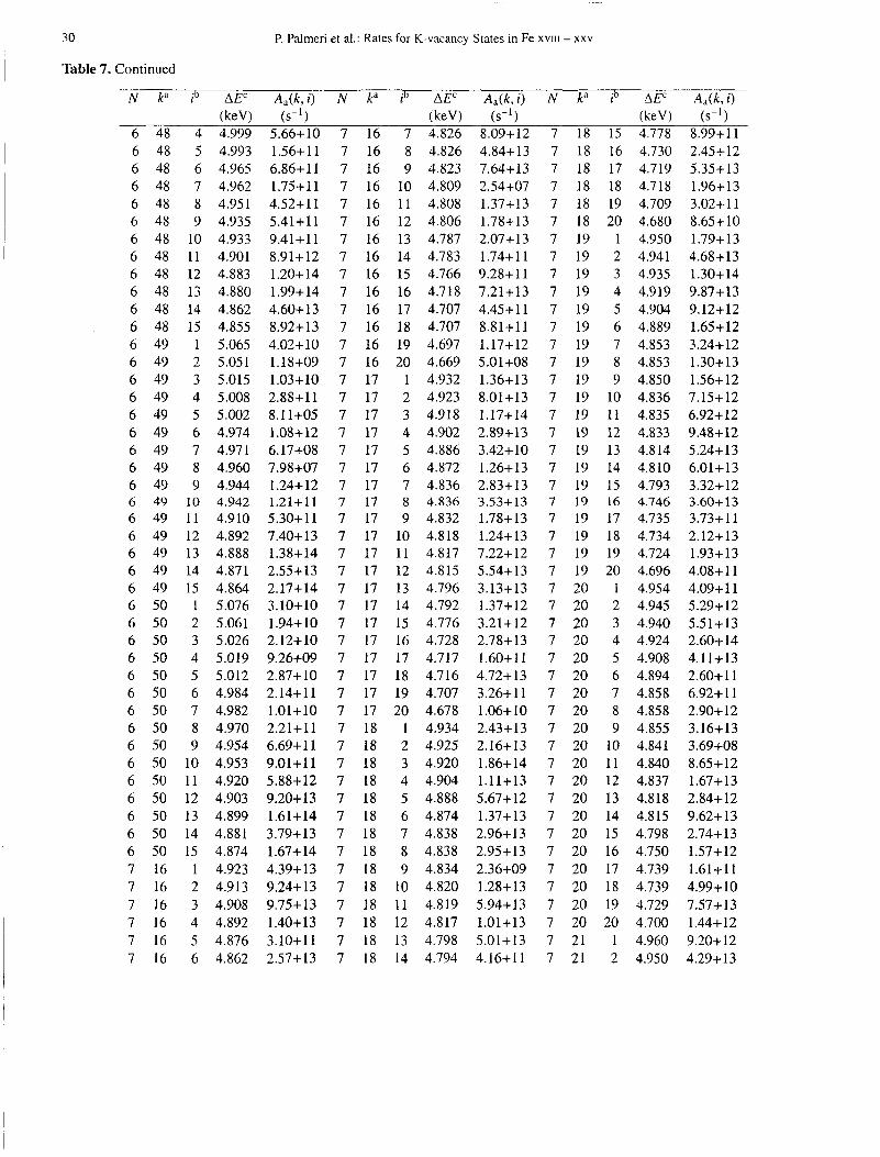
30 P. Palmeri et al.: Rates for K-vacancy States in Fe XVIII - xxv
Table 7. Continued
N k i l ib
6 48 4 6 48 5 6 48 6 6 48 7 6 48 8 6 48 9 6 48 10 6 48 11 6 48 12 6 48 13 6 48 14 6 48 15 6 49 1 6 49 2 6 49 3 6 49 4 6 49 5 6 49 6 6 49 7 6 49 8 6 49 9 6 49 10 6 49 11 6 49 12 6 49 13 6 49 14 6 49 15 6 50 1 6 50 2 6 50 3 6 50 4 6 50 5 6 50 6 6 50 7 6 50 8 6 50 9 6 50 10 6 50 11 6 50 12 6 50 13 6 50 14 6 50 15 7 16 1 7 16 2 7 16 3 7 16 4 7 16 5 7 16 6
AEC (keV) 4.999 4.993 4.965 4.962 4.95 1 4.935 4.933 4.901 4.883 4.880 4.862 4.855 5.065 5.05 1 5.015 5.008 5.002 4.974 4.97 1 4.960 4.944 4.942 4.910 4.892 4.888 4.871 4.864 5.076 5.06 1 5.026 5.019 5.012 4.984 4.982 4.970 4.954 4.953 4.920 4.903 4.899 4.881 4.874 4.923 4.9 13 4.908 4.892 4.876 4.862
W1) 5.66+10 1.56+11 6.86+11 1.75+11 4.52+11 5.41+11 9.41+11 8.91+12 1.20+14 1.99+ 14 4.60+ 13 8.92+13 4.02+10 1.18+09 1.03+ 10 2.88+11 8.11+05 1.08+12 6.17+08 7.98+07 1.24+ 12 1.21+11 5.30+11 7.40+ 13 1.38+ 14 2.55+13 2.17+14 3.10+10 1.94+10 2.12+ 10 9.26+09 2.87+10 2.14+11 1.01+10 2.21+11 6.69+11 9.01+11 5.88+12 9.20+ 13 1.61+14 3.79+13 1.67+14 4.39+ 13 9.24+ 13 9.75+13 1.40+13 3.10+11 2.57+13
N ka ib
7 16 7 7 16 8 7 16 9 7 16 10 7 16 11 7 16 12 7 16 13 7 16 14 7 16 15 7 16 16 7 16 17 7 16 18 7 16 19 7 16 20 7 17 1 7 17 2 7 17 3 7 17 4 7 17 5 7 17 6 7 17 7 7 17 8 7 17 9 7 17 10 7 17 11 7 17 12 7 17 13 7 17 14 7 17 15 7 17 16 7 17 17 7 17 18 7 17 19 7 17 20 7 18 1 7 18 2 7 18 3 7 18 4 7 18 5 7 18 6 7 18 7 7 18 8 7 18 9 7 18 10 7 18 11 7 18 12 7 18 13 7 18 14
AEC (keV) 4.826 4.826 4.823 4.809 4.808 4.806 4.787 4.783 4.766 4.718 4.707 4.707 4.697 4.669 4.932 4.923 4.9 18 4.902 4.886 4.872 4.836 4.836 4.832 4.8 18 4.817 4.815 4.796 4.792 4.776 4.728 4.717 4.716 4.707 4.678 4.934 4.925 4.920 4.904 4.888 4.874 4.838 4.838 4.834 4.820 4.819 4.817 4.798 4.794
8.09+12 4.84+13 7.64+13 2.54+07 1.37+13 1.78+13 2.07+13 1.74+11 9.28+11 7.21+13 4.45+ 1 1 8.81+11 1.17+12 5 .O 1 +08 1.36+13 8.01+13 1.17+14 2.89+13 3.42+10 1.26+13 2.83+ 13 3.53+13 1.78+13 1.24+ 13 7.22+12 5.54+13 3.13+13 1.37+ 12 3.21+12 2.78+13 1.60+11 4.72+ 13 3.26+ 1 1 1.06+10 2.43+13 2.16+13 1.86+14 1.11+13 5.67+12 1.37+ 13 2.96+ 13 2.95+13 2.36+09 1.28+13 5.94+13 1.01+ 13 5.01+13 4.16+11
- N
- 7 7 7 7 7 7 7 7 7 7 7 7 7 7 7 7 7 7 7 7 7 7 7 7 7 7 7 7 7 7 7 7 7 7 7 7 7 7 7 7 7 7 7 7 7 7 7 7
L_
18 18 18 18 18 18 19 19 19 19 19 19 19 19 19 19 19 19 19 19 19 19 19 19 19 19 20 20 20 20 20 20 20 20 20 20 20 20 20 20 20 20 20 20 20 20 21 21
- 15 16 17 18 19 20
1 2 3 4 5 6 7 8 9
10 11 12 13 14 15 16 17 18 19 20
1 2 3 4 5 6 7 8 9
10 11 12 13 14 15 16 17 18 19 20
1 2
AEC (keV) 4.778 4.730 4.719 4.718 4.709 4.680 4.950 4.941 4.935 4.919 4.904 4.889 4.853 4.853 4.850 4.836 4.835 4.833 4.814 4.8 10 4.793 4.746 4.735 4.734 4.724 4.696 4.954 4.945 4.940 4.924 4.908 4.894 4.858 4.858 4.855 4.841 4.840 4.837 4.818 4.815 4.798 4.750 4.739 4.739 4.729 4.700 4.960 4.950
A , ( k i) (S - I )
8.99+ 1 1 2.45+12 5.35+13 1.96+13 3.02+11 8.65+10 1.79+ 13 4.68+13 1.30+14 9.87+13 9.12+12 1.65+12 3.24+12 1.30+13 1.56+ 12 7.15+12 6.92+ 12 9.48+12 5.24+13 6.01 +13 3.32+12 3.60-t 13 3.73+11 2.12+13 1.93+13 4.08+11 4.09+11 5.29+12 5.51+13 2.60+ 14 4.11+13 2.60+ 1 1 6.92+11 2.90+12 3.16+13 3.69+08 8.65+12 1.67+ 13 2,84+12 9.62+13 2.74+ 13 1.57+12 1.61+11 4.99+10 7.57+13 1.44+12 9.20+12 4.29+13

P. Palmeri et al.: Rates for K-vacancy States in Fe XVUI - xxv
Table 7. Continued
31
N k' ib
7 21 3 7 21 4 7 21 5 7 21 6 7 21 7 7 21 8 7 21 9 7 21 10 7 21 11 7 21 12 7 21 13 7 21 14 7 21 15 7 21 16 7 21 17 7 21 18 7 21 19 7 21 20 7 22 1 7 22 2 7 22 3 7 22 4 7 22 5 7 22 6 7 22 7 7 22 8 7 22 9 7 22 10 7 22 11 7 22 12 7 22 13 7 22 14 7 22 15 7 22 16 7 22 17 7 22 18 7 22 19 7 22 20 7 23 1 7 23 2 7 23 3 7 23 4 7 23 5 7 23 6 7 23 7 7 23 8 7 23 9 7 23 10
AEC
4.929 4.9 13 4.899 4.863 4.863 4.860 4.846 4.845 4.843 4.824 4.820 4.803 4.755 4.744 4.744 4.734 4.706 4.961 4.95 1 4.946 4.930 4.914 4.900 4.864 4.864 4.861 4.847 4.846 4.844 4.825 4.821 4.804 4.756 4.745 4.745 4.735 4.707 4.976 4.967 4.961 4.945 4.930 4.915 4.879 4.879 4.876 4.862
A a ( k i) (s-')
1.27+ 14 6.03+13 2.73+13 1.62+ 10 1.09+12 2.3 3 +09 3.05+09 1 .oo+ 1 1 1.03+13 3.25-t 13 5.00+ 13 4.41+12 5.07+13 1.93+12 1.46+13 4.64+ 13 2.06+12 1.31+13 7.00+12 4.62+ 13 3.14+13 1.74+14 3.29+13 3.31+11 8.96+12 7.34+12 2.56+11 6.67+11 1.93+ 1 1 3.58+12 2.88+13 5.76+13 4.38+13 1.31+13 8.45+06 7.06+12 5.75+ 13 1.04+12 2.15+11 9.68+12 2.06+13 1.86+14 6.61+13 2.49+ 1 1 2.71+12 5.20+ 11 1.58+09 2.64+ 12
- N
_.
7 7 7 7 7 7 7 7 7 7 7 7 7 7 7 7 7 7 7 7 7 7 7 7 7 7 7 7 7 7 7 7 7 7 7 7 7 7 7 7 7 7 7 7 7 7 7 7
- k l
23 23 23 23 23 23 23 23 23 23 24 24 24 24 24 24 24 24 24 24 24 24 24 24 24 24 24 24 24 24 25 25 25 25 25 25 25 25 25 25 25 25 25 25 25 25 25 25
- ib -
11 12 13 14 15 16 17 18 19 20
1 2 3 4 5 6 7 8 9
10 11 12 13 14 15 16 17 18 19 20
1 2 3 4 5 6 7 8 9
10 11 12 13 14 15 16 17 18
AEC (keV) 4.861 4.859 4.840 4.836 4.819 4.772 4.761 4.760 4.750 4.722 5.016 5.007 5 .OO 1 4.986 4.970 4.955 4.920 4.919 4.916 4.902 4.901 4.899 4.880 4.876 4.859 4.812 4.801 4.800 4.791 4.762 5.023 5.014 5.009 4.993 4.977 4.963 4.927 4.927 4.924 4.910 4.909 4.907 4.888 4.884 4.867 4.819 4.808 4.808
Aa(k, 0 W1)
7.50+ 12 7.21+12 1.07+ 13 1.33+13 1.14+14 2.46+ 1 1 5.49+12 9.5 1+ 12 6.39+ 12 5.92+13 8.09+06 5.87+10 1.55+11 9.00+10 8.25+06 3.83+12 5.42+13 1.57+14 1.75+14 2.12+ 13 1.84+13 2.82+13 2.88+12 3.93+12 5.40+10 2.01+13 3.57+08 6.48+ 12 1.5 1+ 12 1.40+08 6.32+10 6.39+10 1.07+11 7.03+10 1.11+09 1.99+ 12 8.44+ 13 3.7 1 + 13 1.52+ 14 6.21+12 8.84+13 8.78+13 1.80+ 12 1.22+ 12 1.63+ 12 1.46+13 6.44+ 12 7.09+12
- N
- 7 7 7 7 7 7 7 7 7 7 7 7 7 7 7 7 7 7 7 7 7 7 7 7 7 7 7 7 7 7 7 7 7 7 7 7 7 7 7 7 7 7 7 7 7 7 7 7
ka
25 25 26 26 26 26 26 26 26 26 26 26 26 26 26 26 26 26 26 26 26 26 27 27 27 27 27 27 27 27 27 27 27 27 27 27 27 27 27 27 27 27 28 28 28 28 28 28
ib AEc
19 4.798 20 4.769
1 5.030 2 5.021 3 5.015 4 5.000 5 4.984 6 4.970 7 4.934 8 4.933 9 4.930
10 4.916 11 4.915 12 4.913 13 4.894 14 4.890 15 4.874 16 4.826 17 4.815 18 4.814 19 4.805 20 4.776
1 5.053 2 5.044 3 5.038 4 5.022 5 5.007 6 4.992 7 4.956 8 4.956 9 4.953
10 4.939 11 4.938 12 4.936 13 4.917 14 4.913 15 4.896 16 4.849 17 4.838 18 4.837 19 4.827 20 4.799
1 5.057 2 5.048 3 5.043 4 5.027 5 5.011 6 4.997
(keV) A , ( k i) W')
9.61+11 2.89+ 11 3.41 + 10 1.64+11 3.95+10 4.32+10 3.13+09 1.18+12 3.27+13 8.46+13 6.39+13 2.13+13 4.65+13 1.96+14 7.62+11 8.16+12 9.85+11 7.02 + 1 2 3.42+12 1.80+13 7.89+10 4.69+10 1.57+11 3.65+11 7.53+11 7.89+11 1.33+11 4.05+12 5.72+13 1.12+14 1.72+14 1.55t-13 4.34+13 4.78+13 3.34+12 5.07+12 1.46+12 1.31 +14 1,78+13 4.99+13 3.88+13 1.66+ 12 1,29+11 3.99+11 1.45+11 9.19+10 118+10 2.15+12
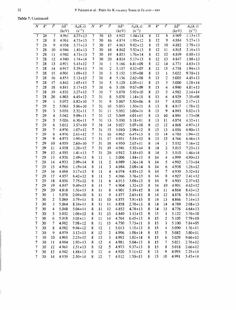
32 P. Palmeri et al.: Rates for K-vacancy States in Fe XVIII - xxv
Table 7. Continued
N k1 ib
7 28 7 7 28 8 7 28 9 7 28 10 7 28 11 7 28 12 7 28 13 7 28 14 7 28 15 7 28 16 7 28 17 7 28 18 7 28 19 7 28 20 7 29 1 7 29 2 7 29 3 7 29 4 7 29 5 7 29 6 7 29 7 7 29 8 7 29 9 7 29 10 7 29 11 7 29 12 7 29 13 7 29 14 7 29 15 7 29 16 7 29 17 7 29 18 7 29 19 7 29 20 7 30 1 7 30 2 7 30 3 7 30 4 7 30 5 7 30 6 7 30 7 7 30 8 7 30 9 7 30 10 7 30 11 7 30 12 7 30 13 7 30 14
AEC
4.961 4.961 4.958 4.944 4.942 4.940 4.92 1 4.917 4.901 4.853 4.842 4.841 4.832 4.803 5.072 5.063 5.058 5.042 5.026 5.012 4.976 4.976 4.973 4.959 4.958 4.955 4.936 4.933 4.916 4.868 4.857 4.856 4.847 4.818 5.078 5.069 5.064 5.048 5.032 5.018 4.982 4.982 4.979 4.965 4.964 4.961 4.942 4.939
(keV A , ( k , i ) N
4.37+13 7 4.73+13 7 5.77+13 7 1.43+13 7 4.73+13 7 1.74+14 7 5.43+12 7 5.29+13 7 1.69+13 7 2.13+13 7 1.65+13 7 5.17+13 7 3.27+12 7 4.45+12 7 8.82+10 7 5.06+10 7 2.32+11 7 9.09+11 7 6.30+11 7 3.57+10 7 1.07+12 7 2.61+12 7 1.95+12 7 2.60+10 7 1.28+12 7 1.41+13 7 2.49+13 8 2.99+14 8 1.19+14 8 3.17+13 8 6.42+12 8 7.75+12 8 9.49+13 8 1.56+13 8 2.09+10 8 3.79+11 8 8.34+11 8 5.04+11 8 1.06+12 8 3.05+11 8 7.98+12 8 9.94+12 8 3.12+13 8 2.23+12 8 1.93+13 8 1.51+13 8 1.88+13 8 2.50+14 8
(S-I)
ka ib
30 15 30 16 30 17 30 18 30 19 30 20 31 1 31 2 31 3 31 4 31 5 31 6 31 7 31 8 31 9 31 10 31 11 31 12 31 13 31 14 31 15 31 16 31 17 31 18 31 19 31 20 11 1 11 2 11 3 11 4 11 5 11 6 11 7 11 8 11 9 11 10 11 11 11 12 11 13 11 14 11 15 12 1 12 2 12 3 12 4 12 5 12 6 12 7
AEC
4.922 4.874 4.863 4.862 4.853 4.824 5.166 5.157 5.152 5.136 5.120 5.106 5.070 5.070 5.067 5.053 5.052 5.049 5.030 5.027 5.010 4.962 4.95 1 4.950 4.941 4.912 5.006 4.989 4.984 4.974 4.966 4.913 4.904 4.901 4.877 4.875 4.858 4.852 4.840 4.764 4.750 5.013 4.996 4.992 4.98 1 4.973 4.920 4.912
( k e V A,@, i)
1.04+ 14 1.95+12 9.02+12 5.52+13 1.76+14 5.17+13 6.8 1 +09 4.52+07 1.95+08 2.62+08 1.05+11 9.67 +09 5.92+10 1.14+11 5.50+06 1.50+11 3.00+11 4.01+11 5.18+11 5.07+10 2.99+12 6.47+13 5.54+12 2.67+ 1 1 5.52+14 3.18+13 1.84+ 13 1.36+ 14 2.09+ 14 4.85+ 13 3.76+ 13 3.09+13 1.32+13 5.19+12 2.63+13 7.91+13 2.70+ 13 4.78+13 1.13+ 12 6.45+13 7.73+11 1.15+13 1.08+14 1.82+ 14 5.04+13 9.37+13 5.11+12 1.50+13
(s-') N k" ib
8 12 8 8 12 9 8 12 10 8 12 11 8 12 12 8 12 13 8 12 14 8 12 15 8 13 1 8 13 2 8 13 3 8 13 4 8 13 5 8 13 6 8 13 7 8 13 8 8 13 9 8 13 10 8 13 11 8 13 12 8 13 13 8 13 14 8 13 15 8 14 1 8 14 2 8 14 3 8 14 4 8 14 5 8 14 6 8 14 7 8 14 8 8 14 9 8 14 10 8 14 11 8 14 12 8 14 13 8 14 14 8 14 15 8 15 1 8 15 2 8 15 3 8 15 4 8 15 5 8 15 6 8 15 7 8 15 8 8 15 9 8 15 10
AEC (keV) 4.909 4.884 4.882 4.865 4.859 4.847 4.77 1 4.758 5.022 5.005 5 .OOO 4.990 4.982 4.929 4.920 4.917 4.893 4.891 4.874 4.868 4.856 4.780 4.766 5.032 5.015 5.010 4.999 4.992 4.938 4.930 4.927 4.903 4.901 4.884 4.878 4.866 4.789 4.776 5.122 5.105 5.100 5.090 5.082 5.029 5.021 5.018 4.993 4.99 1
A& i)
1.13+13 5.27+13 2.79+ 13 2.16+13 6.88+ 13 1.88+ 13 4.63+ 13 1.94+13 9.70+ 1 1 4.45+13 1.28+14 4.81 +13 2.14+14 7.35+08 2.17+13 1.78+12 8.02+13 1.73+08 4.32+11 4.97+ 13 6.90+13 1.94+12 6.46+13 7.16+12 7.23+13 1.46+14 4.90+ 13 1.73+14 1.26+12 5.32+11 2.4 1 + 12 2.37+12 4.62+ 12 8.43+12 9.35+13 7.14+13 2.08+13 4.64+13 3.76+10 7.79+10 7.84+05 1.76+ 1 1 3.80+11 9.66+ 12 2.76+12 2.66+ 12 2.25+14 3.45+14
(s-')
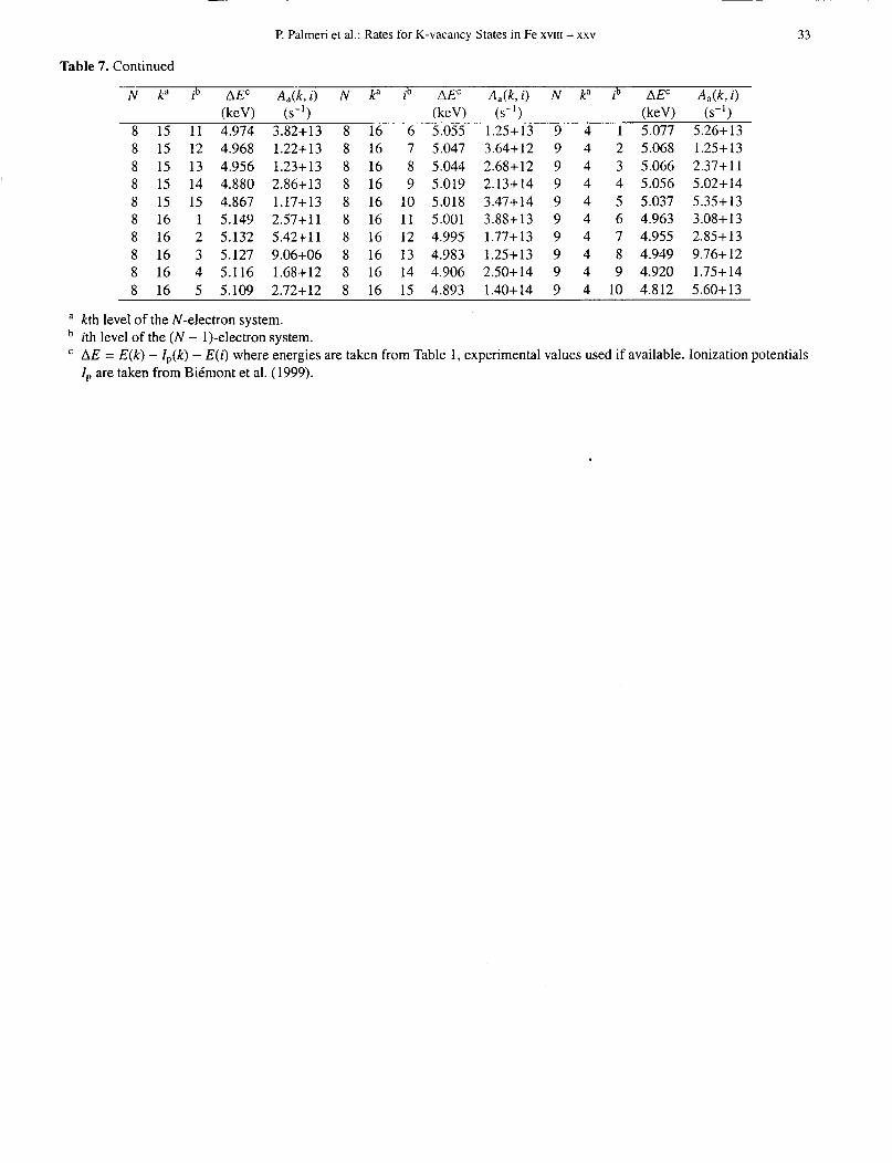
P. Palmeri et al.: Rates for K-vacancy States in Fe X V I I I - xxv
Table 7. Continued
N k" ib AEC A,(k,i) N k" ib AEC A,(k,i) N k" ib AEC A,(k,i)
8 15 11 4.974 3.82+13 8 16 6 5.055 1.25+13 9 4 1 5.077 5.26+13 8 15 12 4.968 1.22+13 8 16 7 5.047 3.64+12 9 4 2 5.068 1.25+13 8 15 13 4.956 1.23+13 8 16 8 5.044 2.68+12 9 4 3 5.066 2.37+11 8 15 14 4.880 2.86+13 8 16 9 5.019 2.13+14 9 4 4 5.056 5.02+14 8 15 15 4.867 1.17+13 8 16 10 5.018 3.47+14 9 4 5 5.037 5.35+13 8 16 1 5.149 2.57+11 8 16 11 5.001 3.88+13 9 4 6 4.963 3.08+13 8 16 2 5.132 5.42+11 8 16 12 4.995 1.77+13 9 4 7 4.955 2.85+13 8 16 3 5.127 9.06+06 8 16 13 4.983 1.25+13 9 4 8 4.949 9.76+12 8 16 4 5.116 1.68+12 8 16 14 4.906 2.50+14 9 4 9 4.920 1.75+14 8 16 5 5.109 2.72+12 8 16 15 4.893 1.40+14 9 4 10 4.812 5.60+13
(keV) (s-') (keV) (s-l) (keV) (s-l)
33
kth level of the N-electron system. ith level of the (N - 1)-electron system. AE = E(k) - ZJk) - E(i) where energies are taken from Table 1, experimental values used if available. Ionization potentials Zp are taken from Bikmont et al. (1999).