a compiler framework for loop nest software-pipelining · a compiler framework for loop nest...

A COMPILER FRAMEWORK

FOR LOOP NEST SOFTWARE-PIPELINING

by

Alban Douillet

A dissertation submitted to the Faculty of the University of Delaware in partialfulfillment of the requirements for the degree of Doctor of Philosophy in Computer Sci-ence

Summer 2006

c© 2006 Alban DouilletAll Rights Reserved

A COMPILER FRAMEWORK

FOR LOOP NEST SOFTWARE-PIPELINING

by

Alban Douillet

Approved:B. David Saunders, Ph.D.Chair of the Department of Computer and Information Sciences

Approved:Thomas M. Apple, Ph.D.Dean of the College of Arts and Sciences

Approved:Conrado M. Gempesaw II, Ph.D.Vice Provost for Academic and International Programs

I certify that I have read this dissertation and that in my opinion it meets theacademic and professional standard required by the University as a dissertationfor the degree of Doctor of Philosophy.

Signed:Guang R. Gao, Ph.D.Professor in charge of dissertation


Signed:Lori Pollock, Ph.D.Professor in charge of dissertation


Signed:Martin Swany, Ph.D.Member of dissertation committee


Signed:Fouad Kiamilev, Ph.D.Member of dissertation committee

ACKNOWLEDGEMENTS

I would like to acknowledge my advisor, Prof. Guang R. Gao, for his support

during those years. He allowed me to work in very favorable conditions while made sure

that I had all the help I needed. His many pieces of advice always happened to be helpful

both on a professional and on a personal level.

This work would have never happened without Dr. Hongbo Rong. He let me work

with him on the SSP project in its early phases and then let me develop my own line of

research. I will always be grateful for his patience during our many heated discussions.

He taught me a lot about persevering and believing in your own work. He also set the bar

higher than I would have myself and motivated me to reach it and go beyond.

Such a large project would not have been possible without the participation of

others. First Dr. Shuxin Yang for porting the Open64 compiler to the IBM Cyclops

architecture in such a short time. Then Juan del Cuvillo for his very helpful answers to

my questions about the architecture. Finally the rest of the Cyclops development team at

ETI including Dr. Ziang Hu, Dr. Haiping Wu, and Weirong Zhu.

I also would like to thank my family for supporting me during all those years.

Despite the distance, they always approved any of my decisions.

Finally my girlfriend, Nina Hansen, was very supportive during the last busy

months of the writing. She showed me the bright side in everything and always kept

me in good spirits.

iv

In memory of my grandfathers Georges Douillet and Charles Binaux.

v

TABLE OF CONTENTS

LIST OF FIGURES . . . . . . . . . . . . . . . . . . . . . . . . . . . . . . . . xivLIST OF TABLES . . . . . . . . . . . . . . . . . . . . . . . . . . . . . . . . . xxiABSTRACT . . . . . . . . . . . . . . . . . . . . . . . . . . . . . . . . . . . . . xxii

Chapter

1 INTRODUCTION . . . . . . . . . . . . . . . . . . . . . . . . . . . . . . . 1

1.1 Towards Cellular Architectures . . . . . . . . . . . . . . . . . . . . . . 21.2 Problem Description . . . . . . . . . . . . . . . . . . . . . . . . . . . . 31.3 Contributions . . . . . . . . . . . . . . . . . . . . . . . . . . . . . . . 41.4 Synopsis . . . . . . . . . . . . . . . . . . . . . . . . . . . . . . . . . . 6

2 BACKGROUND . . . . . . . . . . . . . . . . . . . . . . . . . . . . . . . . 8

2.1 Software-Pipelining . . . . . . . . . . . . . . . . . . . . . . . . . . . . 8

2.1.1 Overview . . . . . . . . . . . . . . . . . . . . . . . . . . . . . 82.1.2 Modulo Scheduling . . . . . . . . . . . . . . . . . . . . . . . . 92.1.3 Clustered-VLIW Software-Pipelining . . . . . . . . . . . . . . . 13

2.2 The Intel Itanium architecture . . . . . . . . . . . . . . . . . . . . . . . 13

2.2.1 Features . . . . . . . . . . . . . . . . . . . . . . . . . . . . . . 142.2.2 Experimental Framework . . . . . . . . . . . . . . . . . . . . . 17

2.3 The IBM 64-bit Cyclops Architecture . . . . . . . . . . . . . . . . . . . 19

2.3.1 Generic Cellular Architectures . . . . . . . . . . . . . . . . . . . 192.3.2 The IBM 64-bit Cyclops Architecture . . . . . . . . . . . . . . . 212.3.3 Experimental Framework . . . . . . . . . . . . . . . . . . . . . 23

vi

3 SINGLE-DIMENSION SOFTWARE PIPELINING . . . . . . . . . . . . . 24

3.1 Problem Description . . . . . . . . . . . . . . . . . . . . . . . . . . . . 25

3.1.1 Motivation . . . . . . . . . . . . . . . . . . . . . . . . . . . . . 253.1.2 Problem Statement . . . . . . . . . . . . . . . . . . . . . . . . . 26

3.2 SSP Theory . . . . . . . . . . . . . . . . . . . . . . . . . . . . . . . . 27

3.2.1 Loop Selection . . . . . . . . . . . . . . . . . . . . . . . . . . . 283.2.2 Dependence Graph Simplification . . . . . . . . . . . . . . . . . 283.2.3 One-Dimensional Scheduling . . . . . . . . . . . . . . . . . . . 303.2.4 Multi-Dimensional Scheduling . . . . . . . . . . . . . . . . . . 323.2.5 Properties . . . . . . . . . . . . . . . . . . . . . . . . . . . . . 34

3.3 SSP Implementation . . . . . . . . . . . . . . . . . . . . . . . . . . . . 343.4 Examples & Notations . . . . . . . . . . . . . . . . . . . . . . . . . . . 36

3.4.1 SSP vs. MS Example . . . . . . . . . . . . . . . . . . . . . . . 363.4.2 Double Loop Nest Example . . . . . . . . . . . . . . . . . . . . 393.4.3 Triple Loop Nest Example . . . . . . . . . . . . . . . . . . . . . 433.4.4 Kernel Notations . . . . . . . . . . . . . . . . . . . . . . . . . . 46

3.5 One-Dimensional Schedule Constraints . . . . . . . . . . . . . . . . . . 47

3.5.1 Perfect Loop Nests . . . . . . . . . . . . . . . . . . . . . . . . . 483.5.2 Imperfect Loop Nests & Single Initiation Interval . . . . . . . . . 503.5.3 Imperfect Loop Nests & Multiple Initiation Intervals . . . . . . . 51

3.6 Schedule Function . . . . . . . . . . . . . . . . . . . . . . . . . . . . . 54

3.6.1 Perfect Loop Nests . . . . . . . . . . . . . . . . . . . . . . . . . 543.6.2 Imperfect Loop Nests & Single Initiation Interval . . . . . . . . . 643.6.3 Imperfect Loop Nests & Multiple Initiation Intervals . . . . . . . 73

3.7 Experimental Results . . . . . . . . . . . . . . . . . . . . . . . . . . . 73

3.7.1 Benchmarks . . . . . . . . . . . . . . . . . . . . . . . . . . . . 733.7.2 Execution Time . . . . . . . . . . . . . . . . . . . . . . . . . . 74

vii

3.7.3 Impact of Loop transformations . . . . . . . . . . . . . . . . . . 773.7.4 Cache Misses Analysis . . . . . . . . . . . . . . . . . . . . . . 78

3.8 Related Work . . . . . . . . . . . . . . . . . . . . . . . . . . . . . . . 80

3.8.1 Hierarchical Scheduling . . . . . . . . . . . . . . . . . . . . . . 803.8.2 Software-Pipelining with Loop Nest Optimizations . . . . . . . . 813.8.3 Loop Nest Linear Scheduling . . . . . . . . . . . . . . . . . . . 84

4 LOOP SELECTION . . . . . . . . . . . . . . . . . . . . . . . . . . . . . . 85

4.1 Initiation Interval . . . . . . . . . . . . . . . . . . . . . . . . . . . . . . 85

4.1.1 Recurrence Minimum Initiation Interval . . . . . . . . . . . . . . 864.1.2 Resource Minimum Initiation Interval . . . . . . . . . . . . . . . 87

4.2 Memory Accesses . . . . . . . . . . . . . . . . . . . . . . . . . . . . . 87

5 SCHEDULER . . . . . . . . . . . . . . . . . . . . . . . . . . . . . . . . . 89

5.1 Introduction . . . . . . . . . . . . . . . . . . . . . . . . . . . . . . . . 895.2 Problem Description . . . . . . . . . . . . . . . . . . . . . . . . . . . . 90

5.2.1 Problem Statement . . . . . . . . . . . . . . . . . . . . . . . . . 905.2.2 Issues . . . . . . . . . . . . . . . . . . . . . . . . . . . . . . . 92

5.3 Solution . . . . . . . . . . . . . . . . . . . . . . . . . . . . . . . . . . 93

5.3.1 Overview . . . . . . . . . . . . . . . . . . . . . . . . . . . . . 935.3.2 Scheduling Approaches . . . . . . . . . . . . . . . . . . . . . . 95

5.3.2.1 Flat Approach . . . . . . . . . . . . . . . . . . . . . . 955.3.2.2 Level-by-Level Approach . . . . . . . . . . . . . . . . 965.3.2.3 Hybrid Approach . . . . . . . . . . . . . . . . . . . . 97

5.3.3 Enforcement of the Scheduling Constraints . . . . . . . . . . . . 97

5.3.3.1 Dependence Constraint . . . . . . . . . . . . . . . . . 975.3.3.2 Sequential Constraint . . . . . . . . . . . . . . . . . . 100

viii

5.3.3.3 Innermost Level Separation Constraint . . . . . . . . . 100

5.3.4 Subkernels Integrity . . . . . . . . . . . . . . . . . . . . . . . . 1015.3.5 Scheduling Priority . . . . . . . . . . . . . . . . . . . . . . . . 1015.3.6 Operation Scheduling . . . . . . . . . . . . . . . . . . . . . . . 1025.3.7 Initiation Interval Increment Methods . . . . . . . . . . . . . . . 103

5.4 Experiments . . . . . . . . . . . . . . . . . . . . . . . . . . . . . . . . 103

5.4.1 Comparison of the Scheduling Approaches . . . . . . . . . . . . 1045.4.2 Comparison of the Scheduling Priorities . . . . . . . . . . . . . . 1055.4.3 Comparison of the Initiation Interval Increment Method . . . . . 106

5.5 Related Work . . . . . . . . . . . . . . . . . . . . . . . . . . . . . . . 1075.6 Conclusion . . . . . . . . . . . . . . . . . . . . . . . . . . . . . . . . . 107

6 REGISTER PRESSURE EVALUATION . . . . . . . . . . . . . . . . . . . 109


6.1.1 Motivation . . . . . . . . . . . . . . . . . . . . . . . . . . . . . 1096.1.2 Notations . . . . . . . . . . . . . . . . . . . . . . . . . . . . . 1116.1.3 Problem Statement . . . . . . . . . . . . . . . . . . . . . . . . . 1126.1.4 Issues . . . . . . . . . . . . . . . . . . . . . . . . . . . . . . . 113

6.2 Solution . . . . . . . . . . . . . . . . . . . . . . . . . . . . . . . . . . 114

6.2.1 Overview . . . . . . . . . . . . . . . . . . . . . . . . . . . . . 1146.2.2 Cross-Iteration Lifetimes . . . . . . . . . . . . . . . . . . . . . 1166.2.3 Local Lifetimes . . . . . . . . . . . . . . . . . . . . . . . . . . 1186.2.4 Register Pressure . . . . . . . . . . . . . . . . . . . . . . . . . 1196.2.5 Time Complexity . . . . . . . . . . . . . . . . . . . . . . . . . 122


6.3.1 Register Pressure Computation Time . . . . . . . . . . . . . . . 1236.3.2 Register Pressure . . . . . . . . . . . . . . . . . . . . . . . . . 1256.3.3 Register File Size . . . . . . . . . . . . . . . . . . . . . . . . . 126

ix

7 REGISTER ALLOCATION . . . . . . . . . . . . . . . . . . . . . . . . . . 129

7.1 Introduction . . . . . . . . . . . . . . . . . . . . . . . . . . . . . . . . 1297.2 MS Register Allocation . . . . . . . . . . . . . . . . . . . . . . . . . . 129

7.2.1 Scalar and Vector Lifetimes . . . . . . . . . . . . . . . . . . . . 1307.2.2 Space-Time Cylinder . . . . . . . . . . . . . . . . . . . . . . . 1317.2.3 Problem Formulation . . . . . . . . . . . . . . . . . . . . . . . 1327.2.4 Register Allocation Solution . . . . . . . . . . . . . . . . . . . . 132


7.3.1 SSP Lifetimes Features . . . . . . . . . . . . . . . . . . . . . . 1337.3.2 Problem Formulation . . . . . . . . . . . . . . . . . . . . . . . 1357.3.3 Terminology . . . . . . . . . . . . . . . . . . . . . . . . . . . . 136

7.3.3.1 Dynamic Views of the Lifetimes . . . . . . . . . . . . 1367.3.3.2 Register Distances . . . . . . . . . . . . . . . . . . . 137

7.4 Solution . . . . . . . . . . . . . . . . . . . . . . . . . . . . . . . . . . 141

7.4.1 Overview . . . . . . . . . . . . . . . . . . . . . . . . . . . . . 1417.4.2 Lifetimes Normalization . . . . . . . . . . . . . . . . . . . . . . 1417.4.3 Lifetimes Representation . . . . . . . . . . . . . . . . . . . . . 144

7.4.3.1 Core Parameters . . . . . . . . . . . . . . . . . . . . . 1447.4.3.2 Derived Parameters . . . . . . . . . . . . . . . . . . . 146

7.4.4 Minimum Register Distance Computation . . . . . . . . . . . . . 148

7.4.4.1 Conservative Distance . . . . . . . . . . . . . . . . . . 1487.4.4.2 Aggressive Distance . . . . . . . . . . . . . . . . . . 1517.4.4.3 Property . . . . . . . . . . . . . . . . . . . . . . . . . 154

7.4.5 Lifetimes Insertion . . . . . . . . . . . . . . . . . . . . . . . . . 1547.4.6 Circumference Minimization . . . . . . . . . . . . . . . . . . . 156

x

7.4.7 Time Complexity . . . . . . . . . . . . . . . . . . . . . . . . . 158


7.5.1 Experimental Framework . . . . . . . . . . . . . . . . . . . . . 1587.5.2 Register Requirements . . . . . . . . . . . . . . . . . . . . . . . 1607.5.3 Lifetime Insertion Strategies . . . . . . . . . . . . . . . . . . . . 1627.5.4 Execution Time . . . . . . . . . . . . . . . . . . . . . . . . . . 1627.5.5 Single Loops . . . . . . . . . . . . . . . . . . . . . . . . . . . . 163


8 CODE GENERATION . . . . . . . . . . . . . . . . . . . . . . . . . . . . . 165


8.2.1 Notations . . . . . . . . . . . . . . . . . . . . . . . . . . . . . 166

8.2.1.1 Double Loop Nest . . . . . . . . . . . . . . . . . . . . 1668.2.1.2 Triple or Deeper Loop Nest . . . . . . . . . . . . . . . 168


8.3 Solution . . . . . . . . . . . . . . . . . . . . . . . . . . . . . . . . . . 172

8.3.1 Code Layout . . . . . . . . . . . . . . . . . . . . . . . . . . . . 1728.3.2 Repeating Patterns Emission . . . . . . . . . . . . . . . . . . . . 1748.3.3 Loop Control . . . . . . . . . . . . . . . . . . . . . . . . . . . 1778.3.4 Conditional Execution of Stages . . . . . . . . . . . . . . . . . . 1788.3.5 Loop Counters Initialization . . . . . . . . . . . . . . . . . . . . 1798.3.6 Register Rotation Emulation . . . . . . . . . . . . . . . . . . . . 1798.3.7 Innermost Level Separation Constraint . . . . . . . . . . . . . . 181

8.4 Example . . . . . . . . . . . . . . . . . . . . . . . . . . . . . . . . . . 1838.5 Experimental Results . . . . . . . . . . . . . . . . . . . . . . . . . . . 187

8.5.1 Execution Time . . . . . . . . . . . . . . . . . . . . . . . . . . 1878.5.2 Code Size . . . . . . . . . . . . . . . . . . . . . . . . . . . . . 188

xi

8.5.3 Bundle Density . . . . . . . . . . . . . . . . . . . . . . . . . . 189


9 MULTI-THREADED SSP . . . . . . . . . . . . . . . . . . . . . . . . . . . 191



9.3 Multi-Threaded SSP Theory . . . . . . . . . . . . . . . . . . . . . . . . 193

9.3.1 Multi-Threaded Final Schedule . . . . . . . . . . . . . . . . . . 1939.3.2 Multi-Threaded Schedule Function . . . . . . . . . . . . . . . . 197

9.4 IBM 64-bit Cyclops Implementation . . . . . . . . . . . . . . . . . . . . 200

9.4.1 Overview . . . . . . . . . . . . . . . . . . . . . . . . . . . . . 2009.4.2 Synchronization . . . . . . . . . . . . . . . . . . . . . . . . . . 2009.4.3 Innermost Loop Tiling . . . . . . . . . . . . . . . . . . . . . . . 2039.4.4 Synchronization Bootstrapping . . . . . . . . . . . . . . . . . . 2069.4.5 Cross-Iteration Register Dependences . . . . . . . . . . . . . . . 2079.4.6 Code Generation Algorithms . . . . . . . . . . . . . . . . . . . 2099.4.7 Correctness . . . . . . . . . . . . . . . . . . . . . . . . . . . . 214


9.5.1 Execution Time Speedup . . . . . . . . . . . . . . . . . . . . . 2169.5.2 Loop Tiling Factor . . . . . . . . . . . . . . . . . . . . . . . . . 2179.5.3 Synchronization Stalls . . . . . . . . . . . . . . . . . . . . . . . 2189.5.4 Register Pressure . . . . . . . . . . . . . . . . . . . . . . . . . 218


10 CONCLUSION . . . . . . . . . . . . . . . . . . . . . . . . . . . . . . . . . 222

10.1 Summary . . . . . . . . . . . . . . . . . . . . . . . . . . . . . . . . . . 222

xii

10.2 Future Work . . . . . . . . . . . . . . . . . . . . . . . . . . . . . . . . 225

BIBLIOGRAPHY . . . . . . . . . . . . . . . . . . . . . . . . . . . . . . . . . 227

xiii

LIST OF FIGURES

2.1 Single Loop Example . . . . . . . . . . . . . . . . . . . . . . . . . . 9

2.2 Single Loop Schedule Example . . . . . . . . . . . . . . . . . . . . . 10

2.3 Single Loop MS Schedule Example . . . . . . . . . . . . . . . . . . . 11

2.4 Software-Pipelining for the Itanium Architecture . . . . . . . . . . . . 16

2.5 SSP Implementation in Open64 . . . . . . . . . . . . . . . . . . . . . 18

2.6 Generic Cellular Architecture Example . . . . . . . . . . . . . . . . . 20

2.7 An IBM 64-bit Cyclops Chip . . . . . . . . . . . . . . . . . . . . . . 22

3.1 SSP Theory Framework . . . . . . . . . . . . . . . . . . . . . . . . . 28

3.2 Zero and Positive Dependences in the Iteration Space . . . . . . . . . . 30

3.3 Kernel Example . . . . . . . . . . . . . . . . . . . . . . . . . . . . . 31

3.4 Kernel in the Final Schedule Example if N2 = 1 . . . . . . . . . . . . 31

3.5 Multi-Dimensional Scheduling Example . . . . . . . . . . . . . . . . 33

3.6 The SSP Framework . . . . . . . . . . . . . . . . . . . . . . . . . . . 35

3.7 MS vs. SSP: Loop Nest . . . . . . . . . . . . . . . . . . . . . . . . . 37

3.8 MS vs. SSP: Kernel . . . . . . . . . . . . . . . . . . . . . . . . . . . 37

3.9 MS vs. SSP: MS Schedules . . . . . . . . . . . . . . . . . . . . . . . 38

3.10 MS vs. SSP: SSP Schedule . . . . . . . . . . . . . . . . . . . . . . . 39

xiv

3.11 Double Loop Nest Example: Inputs . . . . . . . . . . . . . . . . . . . 40

3.12 Double Loop Nest Example: Loop Nest After Loop Selection . . . . . 40

3.13 Double Loop Nest Example: 1-D Schedule . . . . . . . . . . . . . . . 41

3.14 Double Loop Nest Example: Final Schedule . . . . . . . . . . . . . . 42

3.15 Triple Loop Nest Example: Kernel . . . . . . . . . . . . . . . . . . . 44

3.16 Triple Loop Nest Example: Schedule . . . . . . . . . . . . . . . . . . 45

3.17 Generic SSP Kernel . . . . . . . . . . . . . . . . . . . . . . . . . . . 46

3.18 1-D Schedule Constraints in the case of Perfect Loop Nests . . . . . . . 48

3.19 Sequential Constraint Example . . . . . . . . . . . . . . . . . . . . . 49

3.20 1-D Schedule Constraints in the Case of Imperfect Loop Nests andSingle Initiation Interval . . . . . . . . . . . . . . . . . . . . . . . . . 50

3.21 1-D Schedule Constraints in the Case of Imperfect Loop Nests andMultiple Initiation Intervals . . . . . . . . . . . . . . . . . . . . . . . 52

3.22 Unused Cycles Computation Examples . . . . . . . . . . . . . . . . . 54

3.23 Perfect Loop Nest: Schedule Example of Operation op at iteration index(5, 1, 1) . . . . . . . . . . . . . . . . . . . . . . . . . . . . . . . . . 55

3.24 Schedule Function for Perfect Loop Nests . . . . . . . . . . . . . . . . 57

3.25 Schedule Function for Imperfect Loop Nests with Single InitiationInterval . . . . . . . . . . . . . . . . . . . . . . . . . . . . . . . . . 65

3.26 Matrix Multiply Speedups . . . . . . . . . . . . . . . . . . . . . . . . 75

3.27 HD Benchmark Speedup . . . . . . . . . . . . . . . . . . . . . . . . 76

3.28 SPEC2000 Benchmarks Speedups . . . . . . . . . . . . . . . . . . . . 77

3.29 Speedup of the jki Variant of MM after Loop Tiling . . . . . . . . . . . 77

xv

3.30 Speedup of the jki Variant of MM after Unroll-and-Jam . . . . . . . . . 78

3.31 Cache Misses Results for the MM Variants . . . . . . . . . . . . . . . 79

3.32 Hierarchical Scheduling vs. Software-Pipelining Example . . . . . . . 82

5.1 1-D Schedule Constraints in the Case of Imperfect Loop Nests andMultiple Initiation Intervals . . . . . . . . . . . . . . . . . . . . . . . 91

5.2 Strict Initiation Rate of Subkernels . . . . . . . . . . . . . . . . . . . 93

5.3 Truncation of Subkernels . . . . . . . . . . . . . . . . . . . . . . . . 93

5.4 Examples of Poor II Increment Decisions . . . . . . . . . . . . . . . . 94

5.5 Scheduling Framework . . . . . . . . . . . . . . . . . . . . . . . . . 95

5.6 Advantage of the Flat Approach over the Level-by-Level Approach . . . 96

5.7 Scheduling Blocks Example . . . . . . . . . . . . . . . . . . . . . . . 100

5.8 Execution Time Speedup vs. Modulo Scheduling . . . . . . . . . . . . 104

5.9 Comparison of the Scheduling Priorities . . . . . . . . . . . . . . . . . 105

5.10 Comparison of the Initiation Interval Increment Methods . . . . . . . . 106

6.1 SSP Framework . . . . . . . . . . . . . . . . . . . . . . . . . . . . . 110

6.2 Scalar Lifetimes Notations Example . . . . . . . . . . . . . . . . . . . 111

6.3 Irregular Pattern of the Scalar Lifetimes . . . . . . . . . . . . . . . . . 113

6.4 Scalar Lifetimes Variance Within Different Instances of the Same Stage 114

6.5 Scalar Lifetimes in the Final Schedule Example . . . . . . . . . . . . . 115

6.6 Cross-Iteration Lifetimes Algorithm . . . . . . . . . . . . . . . . . . . 117

6.7 Cross-Iteration Lifetimes Computation Example . . . . . . . . . . . . 118

xvi

6.8 Local Lifetimes Algorithm . . . . . . . . . . . . . . . . . . . . . . . 120

6.9 Local Lifetimes Computation Example . . . . . . . . . . . . . . . . . 121

6.10 Register Pressure Computation Time . . . . . . . . . . . . . . . . . . 123

6.11 Speedup vs. the Register Allocator . . . . . . . . . . . . . . . . . . . 124

6.12 Register Pressure . . . . . . . . . . . . . . . . . . . . . . . . . . . . 125

6.13 Ration of Loops Amenable to SSP . . . . . . . . . . . . . . . . . . . . 126

6.14 Total Register Pressure and FP/INT Ratio . . . . . . . . . . . . . . . . 127

6.15 FP Register Pressure Progression . . . . . . . . . . . . . . . . . . . . 128

7.1 Vector Lifetime Examples . . . . . . . . . . . . . . . . . . . . . . . . 131

7.2 Space-Time Cylinder with Optimal Register Allocation . . . . . . . . . 132

7.3 Double Loop Nest Example . . . . . . . . . . . . . . . . . . . . . . . 133

7.4 Double Loop Nest Example Schedule with Lifetime of Variant y . . . . 134

7.5 Simplest Form Examples . . . . . . . . . . . . . . . . . . . . . . . . 136

7.6 Ideal Form Examples . . . . . . . . . . . . . . . . . . . . . . . . . . 138

7.7 Final Form Examples . . . . . . . . . . . . . . . . . . . . . . . . . . 139

7.8 Register Distance Example . . . . . . . . . . . . . . . . . . . . . . . 140

7.9 Conservative Solution . . . . . . . . . . . . . . . . . . . . . . . . . . 140

7.10 Aggressive Solution . . . . . . . . . . . . . . . . . . . . . . . . . . . 140

7.11 Register Allocation Algorithm . . . . . . . . . . . . . . . . . . . . . . 141

7.12 Lifetime Normalization Example . . . . . . . . . . . . . . . . . . . . 142

7.13 Lifetime Normalization Algorithm . . . . . . . . . . . . . . . . . . . 143

xvii

7.14 Conservative Distance: Wands . . . . . . . . . . . . . . . . . . . . . . 148

7.15 Conservative Distance Computation . . . . . . . . . . . . . . . . . . . 150

7.16 Conservative Distance Example . . . . . . . . . . . . . . . . . . . . . 150

7.17 Aggressive Distance Computation . . . . . . . . . . . . . . . . . . . . 152

7.18 Aggressive Distance Example . . . . . . . . . . . . . . . . . . . . . . 153

7.19 Lifetime Insertion Algorithm . . . . . . . . . . . . . . . . . . . . . . 155

7.20 Lifetime Insertion Example . . . . . . . . . . . . . . . . . . . . . . . 156

7.21 Circumference Minimization Algorithm . . . . . . . . . . . . . . . . . 157

7.22 Cumulative Distribution of the Register Requirements for the Loop Nestsof Depth 2 or Higher . . . . . . . . . . . . . . . . . . . . . . . . . . . 161

8.1 Double Loop Nest Kernel . . . . . . . . . . . . . . . . . . . . . . . . 166

8.2 Double Loop Nest Final Schedule . . . . . . . . . . . . . . . . . . . . 167

8.3 Triple Loop Nest Kernel . . . . . . . . . . . . . . . . . . . . . . . . . 169

8.4 Triple Loop Nest Schedule . . . . . . . . . . . . . . . . . . . . . . . 170

8.5 Generated Code Skeleton . . . . . . . . . . . . . . . . . . . . . . . . 173

8.6 Patterns Expansion . . . . . . . . . . . . . . . . . . . . . . . . . . . 175

8.7 Stages Emission . . . . . . . . . . . . . . . . . . . . . . . . . . . . . 176

8.8 Register Rotation Emulation Example . . . . . . . . . . . . . . . . . . 181

8.9 Conditional Emission for the Innermost Level Separation Constraint . . 182

8.10 Example Register-Allocated Kernel . . . . . . . . . . . . . . . . . . . 183

8.11 Example Assembly Code . . . . . . . . . . . . . . . . . . . . . . . . 184

xviii

8.12 Example Final Schedule . . . . . . . . . . . . . . . . . . . . . . . . . 185

8.13 Performance Speedup Relatively to MS . . . . . . . . . . . . . . . . . 187

8.14 Code Size Increase Relatively to MS . . . . . . . . . . . . . . . . . . 188

8.15 Bundle Density . . . . . . . . . . . . . . . . . . . . . . . . . . . . . 189

9.1 Multi-Threaded SSP Schedule Example . . . . . . . . . . . . . . . . . 194

9.2 Without Synchronization Delay Example . . . . . . . . . . . . . . . . 196

9.3 With Synchronization Delay Example . . . . . . . . . . . . . . . . . . 197

9.4 Multi-Threaded Schedule Function for Imperfect Loop Nests with SingleInitiation Interval . . . . . . . . . . . . . . . . . . . . . . . . . . . . 199

9.5 The Multi-Threaded Final Schedule on an IBM 64-bit Cyclops chip . . 201

9.6 Synchronization Instructions Pseudo-Code . . . . . . . . . . . . . . . 202

9.7 Multi-Threaded SSP Schedule Control-Flow Graph for a Triple LoopNest . . . . . . . . . . . . . . . . . . . . . . . . . . . . . . . . . . . 203

9.8 Location of the Synchronization Counters . . . . . . . . . . . . . . . . 204

9.9 Synchronization Tiling Example (G=2) . . . . . . . . . . . . . . . . . 205

9.10 Cross-Iteration Register Dependence Example . . . . . . . . . . . . . 208

9.11 Multi-Threaded Code Skeleton . . . . . . . . . . . . . . . . . . . . . 210

9.12 Loop Patterns Expansion . . . . . . . . . . . . . . . . . . . . . . . . 211

9.13 Stage Emission Algorithm . . . . . . . . . . . . . . . . . . . . . . . . 212

9.14 Initialization Code . . . . . . . . . . . . . . . . . . . . . . . . . . . . 213

9.15 Conclusion Code . . . . . . . . . . . . . . . . . . . . . . . . . . . . 214

9.16 Execution Time Absolute Speedup . . . . . . . . . . . . . . . . . . . 216

xix

9.17 Loop Tiling Factor . . . . . . . . . . . . . . . . . . . . . . . . . . . . 217

9.18 Register Pressure . . . . . . . . . . . . . . . . . . . . . . . . . . . . 219

xx

LIST OF TABLES

3.1 Classification of the Multi-Dimensional Dependences . . . . . . . . . . 29

7.1 Register Allocation Parameters Values Example . . . . . . . . . . . . . 144

7.2 Depth of the Tested Loop Nests . . . . . . . . . . . . . . . . . . . . . 159

8.1 Code Generation Issues and Solutions for Both Target Architectures . . 172

xxi

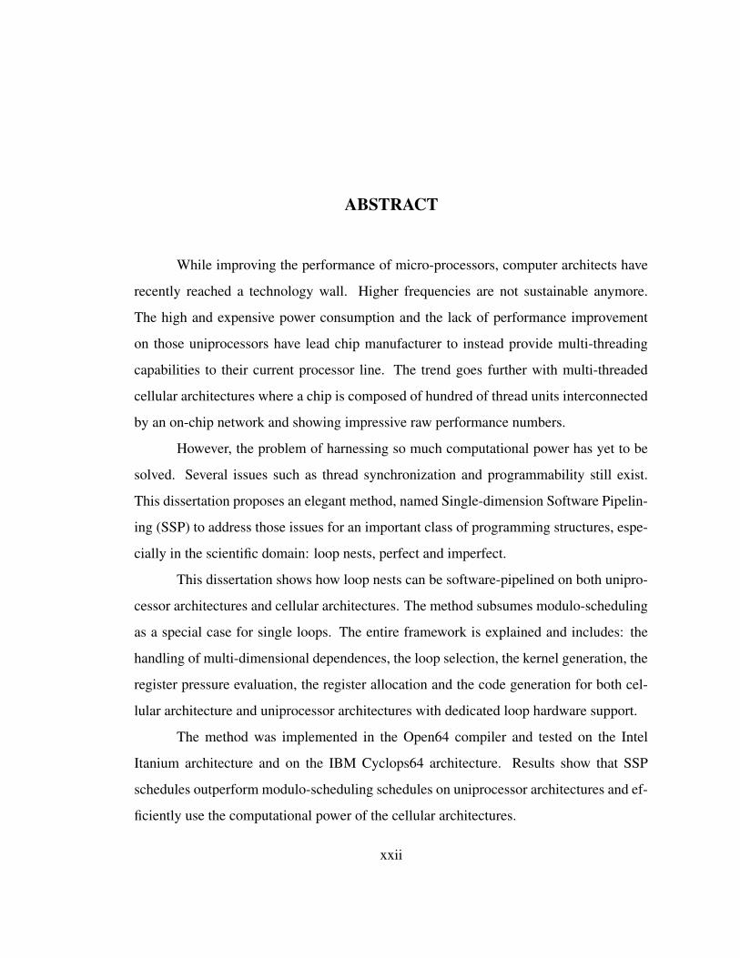
ABSTRACT

While improving the performance of micro-processors, computer architects have

recently reached a technology wall. Higher frequencies are not sustainable anymore.

The high and expensive power consumption and the lack of performance improvement

on those uniprocessors have lead chip manufacturer to instead provide multi-threading

capabilities to their current processor line. The trend goes further with multi-threaded

cellular architectures where a chip is composed of hundred of thread units interconnected

by an on-chip network and showing impressive raw performance numbers.

However, the problem of harnessing so much computational power has yet to be

solved. Several issues such as thread synchronization and programmability still exist.

This dissertation proposes an elegant method, named Single-dimension Software Pipelin-

ing (SSP) to address those issues for an important class of programming structures, espe-

cially in the scientific domain: loop nests, perfect and imperfect.

This dissertation shows how loop nests can be software-pipelined on both unipro-

cessor architectures and cellular architectures. The method subsumes modulo-scheduling

as a special case for single loops. The entire framework is explained and includes: the

handling of multi-dimensional dependences, the loop selection, the kernel generation, the

register pressure evaluation, the register allocation and the code generation for both cel-

lular architecture and uniprocessor architectures with dedicated loop hardware support.

The method was implemented in the Open64 compiler and tested on the Intel

Itanium architecture and on the IBM Cyclops64 architecture. Results show that SSP

schedules outperform modulo-scheduling schedules on uniprocessor architectures and ef-

ficiently use the computational power of the cellular architectures.

xxii

Chapter 1

INTRODUCTION

Parallel processing and data-flow were the buzz words of the 1980’s. Several com-

panies spurred in order to bring to market implementation ideas that had been developed

in research and academic labs. Computer performance was to come from highly parallel

machines. However, the results did not live up to the expectations. All those companies

either went bankrupt or redirected their efforts to dedicated niche markets.

The failure of parallel processing can be explained by several reasons [The99].

Mainly developing a whole new family of processors represents a huge investment which

requires immediate results in order to convince customers to switch to the new architec-

ture. Intel’s recent struggles with the Itanium architecture despite the enormous amount

of investment poured into the project is another example of those difficulties. However

performance is not the only criterion. The main reason behind the lack of success was

the lack of programmability. There was no easy way to extract performance from those

machines. Only institutions with the adequate budget and man power could afford using

this new breed of computers.

To fill the need for more computing power, computer architects turned their efforts

to other types of architectures. A standard von Neumann processor consists of a single

program counter which points to the instruction to be executed. Therefore, the number

of instructions executed per cycle (IPC) never exceeds 1. Increasing the performance of

computers would have to be achieved through going beyond an IPC of 1 and exploit-

ing the instruction level parallelism (ILP). That barrier was breached by the superscalar

1

and VLIW (Very-Long Instruction Word) architectures [HP03]. A superscalar processor

includes several functional units. At run-time, instructions within a given window may

be shuffled from their sequential order in order to be executed as soon as input data are

ready and a functional unit is available. The sequential order semantics is guaranteed.

VLIW processors are similar but the instructions are instead reordered by the compiler.

Instructions that are to be executed in parallel are packed in a single very long instruction

word.

Those two architectures represent the bulk of today’s processors. Unfortunately

the point of diminishing return has been reached. In order to continuously improve the

performance of the processors, architects increased the chip clock speed to unprecedented

levels. Intel even forecast that Xeon processors would be running at more than 10GHz

by the end of the decade. But such a speed comes with a cost. The instructions are

decomposed into micro-instructions and the pipelines of the functional units are made

deeper and deeper. Any interrupt then forces the entire pipeline to be flushed resulting

in an increased waste of precious computing cycles. Also, the use of micro-instructions

only artificially increases the IPC of a processor as the whole original instruction might

actually take longer to execute. Moreover, in order to bridge the performance gap between

the processor and the memory, increasing amounts of cache are moved onto the processor

itself. The result is a chip which computing power is concentrated in a small area. Because

of the high clock speed, that area heats up enormously leading to cooling and power

consumption problems. As a technological wall has been reached, it is now time to move

up to a new type of architecture.

1.1 Towards Cellular Architectures

To cope with the ever increasing power consumption, new architecture classes

were introduced. All have in common the duplication of the processing units within

a single chip. Because the number of transistors on a single chip doubles somewhat

every 18 months, multi-core processing was probably the easiest step towards a more

2

power-friendly solution. As more space on the chip is available, extra processors are

inserted. Each processor is independent from the others with its own L1 cache. They

might share the L2 cache though. As long as there are enough independent tasks to feed

each processor, the computing power of a chip is then a linear function of the number of

processors.

However, the multi-core solution duplicates a large number of functional units

that are continuously dissipating heat. If a processor does not use all of its functional

units at every cycle, that energy is wasted. A solution is to use Simultaneous Multi-

Threading (SMT) [ACC+90, TEL95, TEE+96, CWT+01]. Then several processors share

a pool of functional units. An extra hardware arbiter is in charge of fairly distributing the

instructions of each processor over the available functional units. It is the current solution

used by Intel for the Pentium processor family.

A bigger architectural leap is made with cellular architectures [CCC+02,

ACC+03]. A single chip is composed of one hundred or more thread units. Each thread

unit is a simplified processor with a very limited number of functional units. All the thread

units have access to on-chip shared memory and are interconnected by a network. The

ILP paradigm then shifts to Thread-Level Parallelism (TLP). Such architectures present

several advantages. They consume much less power than the multi-core or SMT archi-

tectures. The heat is evenly distributed through the entire chip. Computing performance

comes from the large number of thread units, not from the processing power of few pro-

cessors. Those chips are also easy and therefore cheaper to manufacture. If few thread

units or memory units are not functional, the chip itself is still functional. The chip design

is highly modular. The number of thread units may vary depending if more memory is

required for instance.

1.2 Problem Description

Therefore cellular architectures are very similar to the paralleling processors pro-

posed in the 1980’s. The large gap between the processors then and today’s cellular

3

architectures has been filled through smooth and economically sound modifications from

one processor generation to the next.

Unfortunately the programmability issues remain untackled: how to harness so

much computational power? How to program applications that will benefit from so much

parallelism? How to synchronize the threads executing on all the thread units? How to

communicate data from one thread to another in a timely fashion? It is the purpose of this

dissertation to propose a solution to these questions for a group of program structures:

loop nests.

Loop nests are present in almost all applications, especially in the scientific do-

main where they can represent 90% of the total execution time of the application. It is

therefore important to ensure their fast execution on any architecture.

The solution proposed in this dissertation, named Single-dimension Software-

Pipelining (SSP) is a complete compilation framework which generates a fully multi-

threaded schedule to execute any imperfect loop nests on cellular architectures. The orig-

inal source code remains unchanged as if the loop nest was to be executed on a unipro-

cessor. Synchronizations between the threads are automatically handled. The framework

includes several steps. In order those are: loop selection, dependences simplification,

kernel generation, register pressure evaluation, register allocation and code generation.

1.3 Contributions

The traditional and most efficient method to schedule a single loop or the

innermost loop of a loop nest on a single processor machine is called software-

pipelining [Lam88]. Rong’s theoretical preliminary work [Ron01] describes the foun-

dation for extending software-pipelining to perfect loop nests on an ideal uniprocessor

architecture. It is the starting point of this work.

The following original contributions are primarily the work of the author:

4

1. The definition and refinement of the level separation constraint for the schedule

functions into the innermost level separation constraint.

2. The design, construction and evaluation of several scheduling methods to generate

the kernel of operations on which an SSP schedule is based.

3. The formulation of an inexpensive but accurate method to evaluate the register pres-

sure of an SSP schedule in order to detect as early as possible infeasible schedules.

4. The specification and evaluation of the code generation scheme for SSP schedules

on cellular architectures with limited dedicated hardware support (rotating regis-

ters).

5. The design of a multi-threaded SSP scheduling solution on cellular architectures.

The solution automatically generates a synchronized software-pipelining schedule

to be executed on a given number of thread units.

The following original contributions are the joint work of the author and Dr. Rong :

5. The formulation of the theoretical schedule functions for perfect and imperfect loop

nests and their properties. The author played a major role in proving the correctness

of those functions.

6. The definition and implementation of heuristics to detect the most profitable loop

level to software pipeline within a loop nest.

7. The specification and evaluation of the code generation scheme for SSP schedules

on VLIW architectures with dedicated hardware support such as rotating registers,

predication, and loop counters.

8. The definition and evaluation of a normalized and complete representation of life-

times in a SSP schedule and a method to use the representation to allocate a mini-

mum of registers to the loop variants of the schedule.

5

1.4 Synopsis

This dissertation is organized as follows:

• The next chapter explains in detail the two target architectures used for the work in

this dissertation. The VLIW architecture is the Itanium architecture, which offers

hardware support for loop execution such as rotating registers, predication and loop

counters. Their usage and the related assembly instructions are detailed there. The

cellular architecture is the IBM 64-bit Cyclops architecture. It features a hundred

thread units and shared memory blocks on a single chip and interconnected by a

cross-bar network. Some useful definitions are also presented.

• Chapter 3 describes the Single-dimension Software-Pipelining (SSP) theory. The

compilation framework is also introduced, followed by the theoretical scheduling

functions. The correctness proofs for perfect and imperfect loop nests and the prop-

erties of SSP schedules are also present. The evaluation of the SSP schedules as

opposed to other loop scheduling methods are shown there.

• Chapter 4 presents two different heuristics to evaluate the most profitable loop level

in a loop nest. That level will be chosen to software-pipeline the loop nest. The first

heuristic is based on resource usage and dependences while the second considers

cache reuse potential.

• Chapter 5 introduces three different methods to generate the one-dimensional SSP

schedule: the kernel. The first method schedules the loop levels one after the other

starting from the innermost. The second schedules all the operations from all the

loop levels simultaneously. The third is an hybrid approach which tries to merge the

advantages of the two other methods. At the end the three methods are evaluated

over a set of benchmarks.

• Chapter 6 shows a fast and accurate solution scheme to evaluate the final register

pressure of the entire SSP schedule by only considering its kernel. If the register

6

pressure is too high, another kernel must be found. The speed and correctness of

the method are also evaluated there.

• Chapter 7 presents the normalized representation of the lifetimes of loop variants

in SSP schedules. This representation is then used to find a register allocation

solution that accommodates all the loop variants of the schedule while minimizing

the register usage. The efficiency of the representation and of the register allocation

solution are tested over a large set of benchmarks. The impact of a solution that

uses no more registers than available is also shown.

• Chapter 8 shows the code generation scheme used for VLIW architectures with

dedicated loop execution hardware support such as register rotation, predication

and loop counter. The method presented shows how to deal with a lack of a multiple

level rotating register file.

• Chapter 9 details the code generation scheme for a single thread unit on cellular

architectures like the IBM 64-bit Cyclops architecture. Then the scheme is extended

to use all the thread units available. The synchronization issues are also handled.

Experimental speedup curves are presented.

• Chapter 10 concludes this dissertation and presents some future work directions.

7

Chapter 2

BACKGROUND

2.1 Software-Pipelining

Because of their repetitive nature, loops represent the most significant part of the

total execution time of programs. Naturally, numerous optimizations, transformations and

scheduling methods have been proposed to reduce the execution time of loops, and soft-

ware pipelining (SWP) is probably the main scheduling method. When applicable, SWP

can be considered as the most powerful scheduling technique for single loops. For a small

cost in code size, SWP makes usage of the machine resources and available instruction-

level parallelism by overlapping the execution of two or more consecutive iterations of

the same loop.

2.1.1 Overview

Typically, without SWP, consecutive iterations of a loop are scheduled one after

the other. Iteration i+1 will start only once iteration i has terminated. Instructions within

a single iteration are scheduled using an instruction scheduler appropriate for the target ar-

chitecture such as list scheduling [Hu61], hyperblock scheduling [MLC+92], superblock

scheduling [WMC+93].

For instance, let us consider the loop example in Figure 2.1 that computes the sum

of the elements of one array and the product of the elements of a second array. Each

operation is assumed to have a latency of 1 cycle and both arrays have a size of N. On any

pipelined non-superscalar architecture and without SWP, the loop is computed as-is using

8

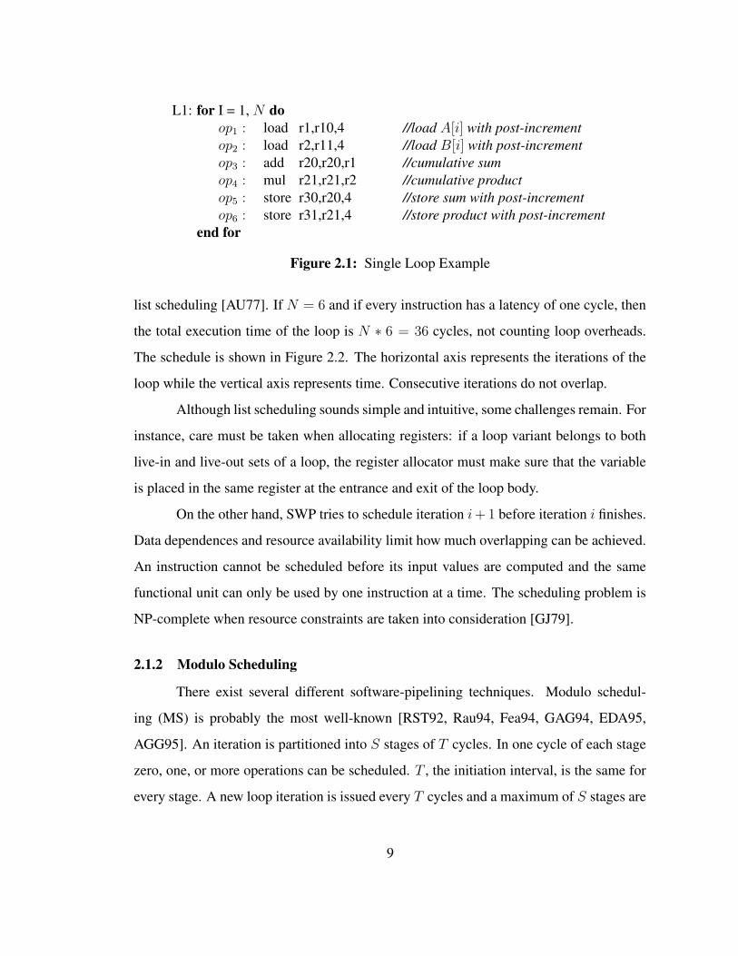
L1: for I = 1, N doop1 : load r1,r10,4 //load A[i] with post-incrementop2 : load r2,r11,4 //load B[i] with post-incrementop3 : add r20,r20,r1 //cumulative sumop4 : mul r21,r21,r2 //cumulative productop5 : store r30,r20,4 //store sum with post-incrementop6 : store r31,r21,4 //store product with post-increment

end for

Figure 2.1: Single Loop Example

list scheduling [AU77]. If N = 6 and if every instruction has a latency of one cycle, then

the total execution time of the loop is N ∗ 6 = 36 cycles, not counting loop overheads.

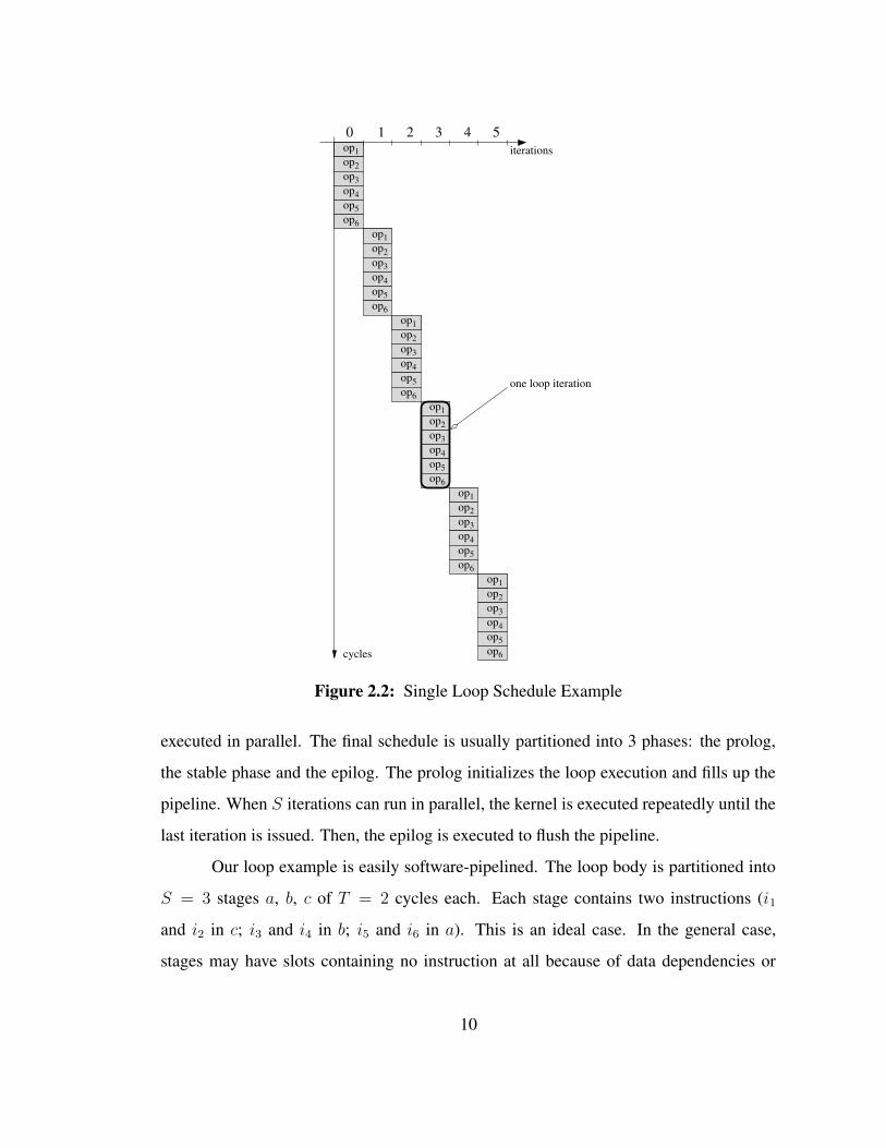
The schedule is shown in Figure 2.2. The horizontal axis represents the iterations of the

loop while the vertical axis represents time. Consecutive iterations do not overlap.

Although list scheduling sounds simple and intuitive, some challenges remain. For

instance, care must be taken when allocating registers: if a loop variant belongs to both

live-in and live-out sets of a loop, the register allocator must make sure that the variable

is placed in the same register at the entrance and exit of the loop body.

On the other hand, SWP tries to schedule iteration i+ 1 before iteration i finishes.

Data dependences and resource availability limit how much overlapping can be achieved.

An instruction cannot be scheduled before its input values are computed and the same

functional unit can only be used by one instruction at a time. The scheduling problem is

NP-complete when resource constraints are taken into consideration [GJ79].

2.1.2 Modulo Scheduling

There exist several different software-pipelining techniques. Modulo schedul-

ing (MS) is probably the most well-known [RST92, Rau94, Fea94, GAG94, EDA95,

AGG95]. An iteration is partitioned into S stages of T cycles. In one cycle of each stage

zero, one, or more operations can be scheduled. T , the initiation interval, is the same for

every stage. A new loop iteration is issued every T cycles and a maximum of S stages are

9

cycles

op1op2op3op4op5op6

op1op2op3op4op5op6

op1op2op3op4op5op6

op1op2op3op4op5op6

op1op2op3op4op5op6

op1op2op3op4op5op6

543210

one loop iteration

iterations

Figure 2.2: Single Loop Schedule Example

executed in parallel. The final schedule is usually partitioned into 3 phases: the prolog,

the stable phase and the epilog. The prolog initializes the loop execution and fills up the

pipeline. When S iterations can run in parallel, the kernel is executed repeatedly until the

last iteration is issued. Then, the epilog is executed to flush the pipeline.

Our loop example is easily software-pipelined. The loop body is partitioned into

S = 3 stages a, b, c of T = 2 cycles each. Each stage contains two instructions (i1

and i2 in c; i3 and i4 in b; i5 and i6 in a). This is an ideal case. In the general case,

stages may have slots containing no instruction at all because of data dependencies or

10

op1op2

op3op4

op5op6

abc

T=2

S=3

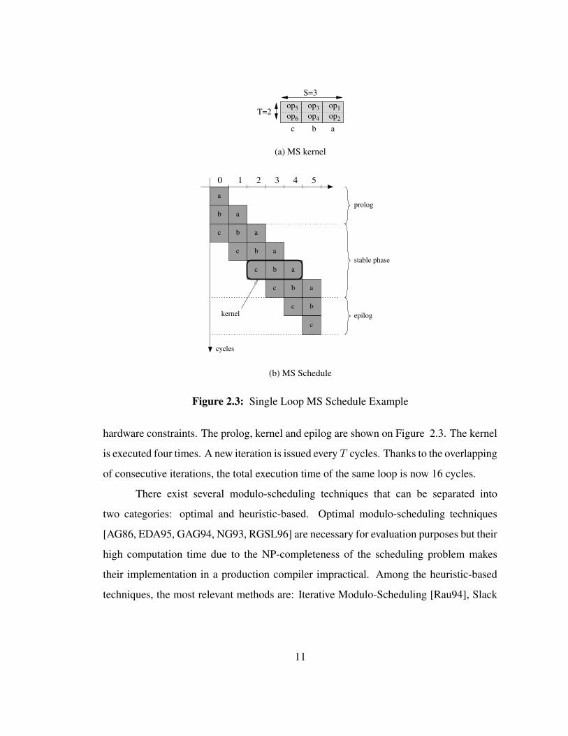
(a) MS kernel

c

b

a

c

b

a

c

b

a

c

b

a

c

b

a

c

b

a

543210

kernel

cycles

prolog

stable phase

epilog

(b) MS Schedule

Figure 2.3: Single Loop MS Schedule Example

hardware constraints. The prolog, kernel and epilog are shown on Figure 2.3. The kernel

is executed four times. A new iteration is issued every T cycles. Thanks to the overlapping

of consecutive iterations, the total execution time of the same loop is now 16 cycles.

There exist several modulo-scheduling techniques that can be separated into

two categories: optimal and heuristic-based. Optimal modulo-scheduling techniques

[AG86, EDA95, GAG94, NG93, RGSL96] are necessary for evaluation purposes but their

high computation time due to the NP-completeness of the scheduling problem makes

their implementation in a production compiler impractical. Among the heuristic-based

techniques, the most relevant methods are: Iterative Modulo-Scheduling [Rau94], Slack

11

Modulo-Scheduling [Huf93], Swing Modulo-Scheduling [LGAV96], Selective Schedul-

ing [ME97] and Integrated Register-Sensitive Iterative Software-Pipelining [DRG98].

For more information about other modulo-scheduling techniques and their relative per-

formance, the reader is referred to [CLG02].

Iterative Modulo-Scheduling [Rau94] sorts operations by height in the data de-

pendency graph and inserts them iteratively into the partial schedule. If a conflict occurs,

then the algorithm backtracks, removes already scheduled operations and reschedules

them in other time slots. The method does not take register assignment into considera-

tion. Integrated Register-Sensitive Iterative Software-Pipelining [DRG98] is an optimized

version of the Iterative Modulo-Scheduling technique that takes into account register pres-

sure.

Slack Modulo-Scheduling [Huf93] sorts operations by slack. The slack of an

operation is the distance between the earliest possible schedule time and the latest possi-

ble schedule time of the operation. An operation on the critical path in the data depen-

dency graph will have a higher priority than an operation on another path. Like Iterative

Modulo-Scheduling, if it is not feasible to schedule the current operation, backtracking

occurs. Because the lifetimes of the loop variants are considered in the process, register

requirements are reduced.

Swing Modulo-Scheduling [LGAV96] does not use backtracking but relies on a

more advanced sorting techniques based on the criticality and recurrence cycle length of

the path to which they belong. The ordering of the nodes also helps to reduce register

requirement. Because this method does not iterate, it is comparably faster than the other

methods.

Selective Scheduling [ME97] is targeted for VLIW processors. The SWP kernel

is a single VLIW instruction word. The instruction starts empty and is filled up with

instructions using global scheduling techniques based on speculative code motion and

target register renaming. The operations that are not scheduled in the kernel are sorted

12

in the prolog and epilog. The technique automatically handles branches within the loop

using speculation and variable initiation intervals.

2.1.3 Clustered-VLIW Software-Pipelining

Clustered-VLIW architectures are very common in the embedded processor world.

In order to compensate for the stagnating wire delays in the faster processors, chip re-

sources such as registers, functional units and memory ports are partitioned into clusters.

Clusters can communicate with each other using a memory bus or a register bus. The

architecture uses VLIW (Very-Long Instruction Word) instruction format. Consequently,

all functional units, even across clusters, share the same clock cycle and advance in a

lock-step mechanism. If one functional unit executes a long-latency operation, all the

other functional units must wait for the operation to be completed, even if their own op-

erations have already been completed.

There exist several methods to software pipeline single loops on such architec-

tures. Fernandes et Al [FLT99] perform both scheduling and partitioning in a single step

on a clustered VLIW architecture with queues to communicate between clusters. Nystrom

and Eichenberger [NE98] proposed an iterative two-step algorithm where scheduling and

partitioning are performed in two separate steps. If no feasible schedule can be found, the

initiation interval is increased. Their method does not seem to scale well when the register

buses become saturated [SG00a]. Sanchez and Gonzales [SG00a, SG00b] proposed an

iterative unified approach that performs scheduling and partitioning in one single step and

tries to minimize inter-cluster communications.

2.2 The Intel Itanium architecture

The Itanium architecture was developed with two ideas in mind: to expose the

instruction-level parallelism of any given program to the compiler and to increase the

number of executed instructions per cycle for server applications (e.g. data-base servers

13

and web servers) [HMR+00]. The choices were made based on academic and indus-

trial research concerning the EPIC (Explicitly Parallel Instruction Computing) architec-

ture [CNO+88, RYYT89, MCmWH+92, GCM+94].

To increase the instruction throughput, a flexible VLIW instruction style is used.

In each cycle an implementation-dependent number of bundles of three instructions each

are fetched. The data size is set to 64 bits as opposed to the current 32-bit machines.

Larger data size means more information computed each cycle and more addressable

memory.

2.2.1 Features

To expose instruction-level parallelism to the compiler, a number of instructions

and hardware support were included in the design [Int01]:

• Predication: Instructions can be predicated so that if-conversion can be performed.

Thanks to if-conversion [AKPW83, DHB89], control dependencies are transformed

into data dependencies, transforming basic blocks into larger hyperblocks and ex-

posing more instruction-level parallelism to the compiler.

• Data Speculation: Load addresses can be speculated to schedule a load as early as

possible, even before the address is known. If an error is made in speculation, some

recovery code is executed.

• Control Speculation: Control speculation allows loads and stores to be executed

before the branch instruction that dominates them. Check instructions are inserted

to recover in case of failed speculation.

• Large register file: A large register file is provided to limit register spills and re-

stores. Spills and restores are load and store instructions that save and restore reg-

ister values to and from the memory when there are not enough registers available

to hold all the values the program is using.

14

• Software-pipelining support: Traditional software-pipelining is highly supported

with the presence of architectural features: loop counter registers, predication, ro-

tating registers, and large register files. All these features increase the range of loops

that can be software-pipelined and eliminate most of the loop control overheads.

For a better understanding and because SSP will be using some of the Itanium

features for its implementation, the example of a single loop is used here. We assume that

the loop body is a single large basic block. The loop body is software-pipelined. Only the

code for the stages of the kernel need to be generated. Let us consider the code from the

Itanium manual [Int01] shown in Figure 2.4.

Two loop counters are used. The lc register is the main loop counter of the loop.

The ec register is the epilog counter. When all the loop iterations have been issued (but

not yet fully executed) and it is time to flush the pipeline, the epilog counter is used to

count how many extra iterations the loop should be executed. The ec value only decre-

ments once the lc value reaches zero. Both counters are decremented when a new loop

iteration is issued using a special branch instruction: br.ctop. The instruction branches,

decrements the loop counters and rotates the rotating registers all in one cycle.

Each stage (and all the instructions in it) is guarded by a predicate register, starting

from p16. The predicate registers rotate when the br.ctop instruction is executed. When

the predicate registers rotate, the value in the predicate register i is copied into the predi-

cate register i+1. As long as lc > 0, p16 is set to 1 during the register rotation. Otherwise

p16 is set to 0. Rotating predicate registers are a very convenient way to fill, run, and flush

the pipeline with a single instance of the kernel instructions.

General-purpose registers above 32 rotate. Therefore, the value stored in r32 after

the load will be in r34 “two executions of br.ctop later” for the add instruction to use.

Rotating registers avoid manual copies of registers that would potentially slow down the

loop execution. The SSP algorithm will make use of all of these features but in a different

manner as described in Section 8.

15

L1: for I = 0, N − 1 dold4 r4=[r5],4;; //load with post-incrementadd r7=r4,r7;; //add cumulative sumst4 [r6]=r7,4;; //store sum with post-increment

end for

(a) Before Software-Pipelining

mov lc=N-1 //LC = loop count - 1mov ec=4 //EC = epilog stages - 1mov pr.rot=1<<16 //p16 = 1, others = 0

L1: (p16) ld4 r32=[r5],4(p18) add r35=r34,r9(p19) st4 [r6]=r36,4

br.ctop L1;;

(b) After Software-Pipelining

ld4

add

st4

ld4

add

st4

ld4

add

ld4

ld4

ld4addst4

st4 add

addst4

st4

Register Values

iterations

0 1 2 3 4 N−1N−2N−3

cycles

LC1

1

1

1 1 1 1

11

1

1

1

1

1

0 0

0

0

0

0

0

0

0

0

0

1 1 1 1

111

1 1

1

3

4

2

1

0 0 0 0 00

0

0

0

0

4

4

4

4

4

0

ECp19p18p17p16

N−2

N−3

N−4

N−5

N−1

(c) Software-Pipelined Schedule

Figure 2.4: Software-Pipelining for the Itanium Architecture

16

2.2.2 Experimental Framework

The Itanium architecture is one of the two target architectures used to collect ex-

perimental data about the SSP method. The SSP framework is implemented in the Open64

compiler [Ope03]. The Open64 compiler is a open-source research compiler using the

GNU Compiler front-ends for C, C++ and Fortran. Originally developed by SGI for its

MIPS processors, it has been retargeted for the Intel Itanium architecture. It includes

several optimizations at every level of the compilation process with profiling support if

necessary.

Open64 uses the Winning Hierarchical Intermediate Representation Language, or

WHIRL, as the representation for all the optimizations. WHIRL uses 5 different levels

of representation from source code level to assembly level. They are named: Very High

(VH), High (H). Middle (M), Low (L) and Very Low (VL). The lower the representation

is, the more details are available for the optimizations. Very high level optimizations

such as inlining are run at the Very High level. At the High level, several optimizations

are performed: Interprocedural Analysis including cloning, inlining, dead function and

variable elimination, and constant propagation; Architecture-independent optimizations

(PreOPT); and Loop Nest Optimizations (LNO), including loop fission, loop fusion, loop

tiling, loop peeling, unroll-and-jam, loop interchange and vector data prefetching. Global

scalar Static-Single Assignment (SSA) optimizations (WOPT) are then used at the Middle

level. Register Variable Identification (RVI) is run both at the Middle and Low levels.

Architecture-dependent optimizations are finally applied at the Low and Very Low levels.

Most of the SSP algorithms are applied at the Very Low level during the code

generation (CG) phase that includes hyperblock formation, global and local scheduling,

global and local register allocation, control-flow optimizations, software-pipelining and

code emission. The data dependence graph analysis steps take place during the LNO

phase at the High representation level. The implementation of SSP within Open64 is

shown in Figure 2.5.

17

GNU Front−EndC/C++/Fortran

Binary Code

Source Code

PreOPT

WOPT

CGVery Low

Low

Middle

High

Very High

WHIRL Levels SSP Framework

Loop Nest

Itanium Code Cyclops64 Code

Dependence Analysis

1−D DDG Loop Level

SSP Kernel

SSP Kernel

SSP KernelRegister−Allocated

Loop Selection

Register Pressure Evaluation

Register Allocation

EPIC MTC

Code Generation

Modulo Scheduling

VHO

IPA

RVI

LNO

Figure 2.5: SSP Implementation in Open64

18

The final schedule in Itanium assembly code is assembled and linked using GNU

tools [gcc03] and is run on an Itanium machine with an Itanium 2 processor running at

1.4GHz equipped with 32KB/256KB/1.5MB of L1/L2/L3 caches and 1GB RAM. The

machine was set to single-user mode to reduce noise in the collected timing results. Also

each experiment was averaged over 3 runs. The measured parameters were execution

time, cache misses, code size, and code density. Correctness was tested against the Ita-

nium GCC compiler.

2.3 The IBM 64-bit Cyclops Architecture

2.3.1 Generic Cellular Architectures

In the past decade, the trend for microprocessor design has been largely driven by

clock speed [BG97, BG04]. The need for faster processors led to deeper pipelines, larger

multi-level on-chip caches, sophisticated branch predictors, register renaming techniques,

speculative execution, etc. However, technology is reaching a point of diminishing re-

turn. Longer and longer memory latencies, increasing wire delays, power consumption,

design complexity and the impossibility to deepen pipelines even further forced computer

architects to look at other directions for improvement. Moreover, although predication

[AKPW83, DHB89] and speculation [CR00] increase processor utilization, the amount

of useful work is still limited.

A counter-approach is to have more than one processor core on a single chip,

but featuring less resources such as functional units: thread-level parallelism replaces

instruction-level parallelism. When pushed to the extreme, this principle leads to a new

type of computer architecture: Multi-Threaded Cellular (MTC) Architecture [CCC+02].

In an MTC architecture, a processor or, more exactly, a thread unit is reduced to a strict

minimum: a program counter, an all-purpose pipelined functional unit and a register file.

There is no scoreboarding, branch predictor or any hardware optimizations implemented.

As for the cache, several memory banks are used. A single cache with several ports

19

would be too expensive to implement and very inefficient as well. Memory banks and

thread units are then connected by a network as shown in Figure 2.6.

PC ALU

RF

PC ALU

RF

...

...

NETWORK

MEM MEM

OFF−C

HIP M

EM

OR

Y

Figure 2.6: Generic Cellular Architecture Example

The are multiple advantages of such an architecture:

• First, from a power consumption point of view, energy is better utilized. Instead of

using large amount of power into hardware optimizations such as branch prediction

to speed up the execution of single thread, that energy is used to execute many

more threads. At the end, the amount of work done for a given amount of energy is

higher [LM05]. Moreover, the use of several thread units spread on the silicon chip

also eases the heat dissipation.

• From a manufacturing point of view, the chip is less expensive to produce. If one

thread unit or memory bank has a defect, the chip is still fully functional. Therefore

there is little silicon waffle waste.

• From a designer point of view, the chip is highly modular. Therefore it is easier to

design, develop and debug. Any subsequent upgrades are less costly.

20

• From a compiler point of view, simple hardware means better understanding of the

processor and therefore better optimization algorithms. The compiler should be

able to more easily harness the performance power of the processor.

• From a financial point of view, the entire design and manufacturing of the chip and

associated development tools, including compilers or operating systems, are sim-

plified resulting in a less expensive computer system. Smaller power consumption

is also deducted from the total bill.

2.3.2 The IBM 64-bit Cyclops Architecture

One instance of an MTC architecture that was used in this dissertation is the IBM

64-bit Cyclops chip [CCC+02, ACC+03, AAC+03], shown in Figure 2.7. The Cyclops

project was originally part of the IBM BlueGene project [IBM03]. The goal is to design

an affordable supercomputer with 1 Teraflop capability. The supercomputer is composed

of several nodes organized in racks and linked together by a 3D-mesh network.

Each node may contain several 64-bit Cyclops chips. A single chip contains 160

thread units and as many memory banks interconnected together with a crossbar network.

Also connected to the network are off-chip memory banks, 6 outer-network connections

for the 3D-mesh network between chips, 1 local SATA hard drive and 1 control channel

for human intervention.

A thread unit is composed of a functional unit for memory, branch and integer

arithmetic operations, a floating-point unit, a private register file, a program counter. For

the purpose of this study, the register file is assumed to be rotating. The floating-point

unit is shared between two thread units. The two thread units and the floating-point unit

forms a processor. Each processor is connected to the crossbar network with a single port.

Access to the crossbar is handled in First-In First-Out (FIFO) order on the sender side.

Data is transferred from the sending port to the receiving port only after the transfer can be

guaranteed free of contention. Memory reads and writes are then handled atomically on

21

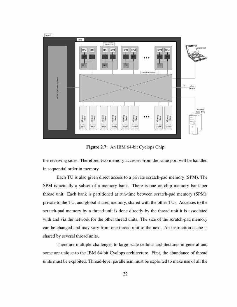
chip

board

Off

−Chi

p M

emor

y B

ank

Ban

kM

emor

y

Ban

kM

emor

y

Ban

kM

emor

y

Ban

kM

emor

y

Ban

kM

emor

y

Ban

kM

emor

y

Ban

kM

emor

y

Ban

kM

emor

y

TU TU

FPU

SPM SPM

TU TU

FPU

SPM SPM

TU TU

FPU

SPM SPM

TU TU

FPU

SPM SPM

processor

crossbar network

boardsother6

terminal

hard driveexternal

SPMSPM SPM SPM SPM SPM SPMSPM

Figure 2.7: An IBM 64-bit Cyclops Chip

the receiving sides. Therefore, two memory accesses from the same port will be handled

in sequential order in memory.

Each TU is also given direct access to a private scratch-pad memory (SPM). The

SPM is actually a subset of a memory bank. There is one on-chip memory bank per

thread unit. Each bank is partitioned at run-time between scratch-pad memory (SPM),

private to the TU, and global shared memory, shared with the other TUs. Accesses to the

scratch-pad memory by a thread unit is done directly by the thread unit it is associated

with and via the network for the other thread units. The size of the scratch-pad memory

can be changed and may vary from one thread unit to the next. An instruction cache is

shared by several thread units.

There are multiple challenges to large-scale cellular architectures in general and

some are unique to the IBM 64-bit Cyclops architecture. First, the abundance of thread

units must be exploited. Thread-level parallelism must be exploited to make use of all the

22

available resources. Second, the workload must be distributed fairly among all the thread

units to avoid execution bottleneck and increase processor utilization. Third, the thread

units must synchronize with each other without impending the flow of execution. High

synchronization costs would result in loss of performance.


The IBM 64-bit Cyclops architecture is the target architecture to collect experi-

mental results about multi-threaded SSP schedules. Similarly to the Itanium architecture,

MT-SSP was implemented into the Open64 compiler which has been retargeted to the

IBM 64-bit Cyclops architecture. The standard GNU utilities, such as assembler and

linker, were then used to produce the final binary file. Again, GCC was used to test the

correctness of the output.

Because the IBM 64-bit Cyclops is still in its development phase, no processor is

available for testing. Instead the benchmarks were run on the simulator [dCZHG05] used

by the IBM 64-bit Cyclops hardware and software development teams. The simulator

was written from the ground up and supports multi-chip multi-threaded execution. It

is functionally-accurate and models the instruction cache, the memory banks, the FIFO

queues and the crossbar network.

23

Chapter 3

SINGLE-DIMENSION SOFTWARE PIPELINING

This chapter presents the Single-dimension Software Pipelining technique, or SSP

for short. An early theoretical work for perfect loop nests on an ideal architecture was

originally proposed by Rong in his Ph.D. dissertation [Ron01]. This chapter extends the

work to imperfect loop nests and proves the correctness of the scheduling functions. The

next chapters show how to apply SSP to real-life architectures. SSP is a methodology to

software pipeline loop nests at an arbitrary level, unlike modulo scheduling which focuses

on the innermost loop only. This chapter presents the method from a theoretical point of

view. It is meant both as an introduction to SSP and as a reference and basis for the next

chapters.

The next sections explain how SSP simplifies the multi-dimensional problem of

scheduling loop nests into a uni-dimensional problem, the solution of which is used to

generate the final multi-dimensional schedule. Section 3.1 gives an overview of the SSP

method. Section 3.2 presents a detailed overview of the SSP theory. The next section

explains how the SSP methodology is actually implemented in practice. To help the

reader, full examples will be presented in Section 3.4. The scheduling constraints used

for the scheduler are explained in Section 3.5 and Section 3.6 presents the final schedule

function for the operations of the loop nests. Section 3.7 will then present some numbers

showing the usefulness of the method.

24


3.1.1 Motivation

From the perspective of improving programs total execution time, several ap-

proaches are possible. With the advent of VLIW and EPIC architectures, exploiting

instruction-level parallelism (ILP) in programs helps improving the overall performance

of applications. For instance, processors such as Intel Itanium [Int01] offer wider and

wider hardware resources to do just that. Moreover loop nests in scientific applications

represent a significant ratio of the total execution time and intrinsically have a high degree

of instruction-level parallelism. Therefore, it is important to carefully design loop nest

scheduling methods that can efficiently extract the ILP present in the multi-dimensional

iteration space of loop nests and expose it to the target architecture.

The main method to extract ILP from loop nests is probably software pipelin-

ing (SWP) [Woo79, Lam88]. SWP schedules the iterations of a loop in paral-

lel while respecting data dependences. Each iteration starts before the previous one

has terminated as in a pipeline, hence the terminology. However, most implementa-

tions [AN88a, AN88b, AN91, AG86, DRG98, Huf93, LGAV96, NG93, ASR95, Cha81,

ME92, EN90, Jai91, RA93, RG81, RST92, Rau94, Fea94, GAG94, EDA95, AGG95],

including the most popular modulo-scheduling (MS), only consider single loops or the in-

nermost loop of a loop nest. Even if loop nest transformations are applied before schedul-

ing the loop nests, the amount of ILP to be extracted is limited to the innermost level.

Also, the data reuse potential in the outer loops cannot be exploited [CK94, CDS96]

There exist several other methods to software pipelining the entire loop nest, but

they all have their drawbacks. Hierarchical scheduling [Lam88, ME97] software pipelines

each loop level separately, starting from the innermost, and considering each one as an

atomic operation for the corresponding enclosing loop. Although attractive by its simplic-

ity, the technique suffers from strong scheduling constraints and gives too much priority

to the innermost loops. Decisions made in the innermost levels are fixed and may hinder

25

the ILP of the loop nest. In [MD01, WG96], the prolog and epilog of the innermost loop

are overlapped. Unfortunately the method can only be used for the innermost level. Loop

nest linear scheduling [DSRV99, DSRV02] was also proposed to schedule operations of a

loop nests using linear functions. However the method does not seem to take into account

hardware constraints such as register files. SSP is the only method to software pipeline a

loop nest while taking into account hardware resources.

Moreover, SSP offers several advantages. First, it is a loop nest scheduling method

which can be seen as a natural generalization of MS to multi-dimensional loops [Ron01,

RTG+03, RTG+04]. SSP retains its simplicity and, when applied to a single loop or to the

innermost loop of a loop nest, SSP is in fact equivalent to MS. Therefore SSP schedules

are at least as good as MS schedules. However, SSP is more flexible and can schedule

other loop levels when judged profitable. Examples in Section 3.4 show how SSP can

outperform MS.

3.1.2 Problem Statement

The problem that the single-dimension software pipelining method addresses can

be formally formulated as follows: Given a loop nest made of n loops L1,. . .,Ln, identify

the most profitable loop Li and software pipeline it. If loop Li is selected and software

pipelined, then its iterations will be executed in parallel. However, the iterations of the

loops Lj enclosed within Li (j > i) will run sequentially within each iteration of Li. The

loops Lk enclosing Li (k < i) are not software pipelined and remain intact. Therefore,

for clarity reasons, we will always ignore the enclosing loops L1, ..., Li−1 and, without

loss of generality, consider the selected loop as the outermost loop level in the loop nest.

In the rest of the dissertation, n will always designate the depth of the loop nest and Li

the loop at level i with n being the deepest level. The number of iterations for each loop

Li will be noted Ni.

Despite the general formulation, SSP currently targets any imperfect loop nests

that fulfills the following criteria. First, there must be no negative dependences at the

26

selected level. Otherwise, no overlapping between iterations is possible. Second, the

loop nests cannot include loop siblings. The loop nests can be imperfect, but may only

include one loop per level. Those loop nests are also called Singly-Nested Loop Nests

(SNLN) [WMC98]. This limitation is not a theoretical but a practical one. The removal

of this constraint is left to future work.

To software pipeline a loop nest, the SSP method must address several issues and

answer some questions: how to define the profitability of a loop level and how to measure

it? How to handle the multi-dimensional dependences of the loop nest? How to take into

account the limited hardware resources of the processor such as registers and functional

units? How to generate a repetitive schedule? How to manage the loop overheads such

as loop counters and branch instructions? Those questions will be answered as the SSP

implementation is explained in the next chapters. The next section gives an overview of

the methodology used.

3.2 SSP Theory

To schedule loop nests, SSP proceeds in four steps shown in Figure 3.1. First,

the loop to software pipeline in the loop nest is selected. The multi-dimensional data

dependence graph (n-D DDG) is then simplified into the one-dimensional data depen-

dence graph (1-D DDG) of the selected loop level. The computed graph is then used to

schedule the operations of the loop nests from the selected loop level and deeper. The

obtained schedule is named the one-dimensional schedule (1-D schedule) of the loop nest

and corresponds to the execution of a single iteration of the selected loop. The hardware

constraints are then taken into consideration to allow the overlapped execution of the other

iterations of the selected level and the final schedule is generated. Each step is described

with more details in the next sections.

27

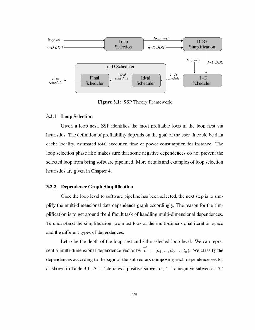
loop nest1−D DDG

n−D DDG

loop nest

finalschedule

scheduleideal

schedule1−D

n−D DDG

loop level

n−D Scheduler

SimplificationDDG

1−DScheduler

IdealScheduler

FinalScheduler

SelectionLoop

Figure 3.1: SSP Theory Framework

3.2.1 Loop Selection

Given a loop nest, SSP identifies the most profitable loop in the loop nest via

heuristics. The definition of profitability depends on the goal of the user. It could be data

cache locality, estimated total execution time or power consumption for instance. The

loop selection phase also makes sure that some negative dependences do not prevent the

selected loop from being software pipelined. More details and examples of loop selection

heuristics are given in Chapter 4.

3.2.2 Dependence Graph Simplification

Once the loop level to software pipeline has been selected, the next step is to sim-

plify the multi-dimensional data dependence graph accordingly. The reason for the sim-

plification is to get around the difficult task of handling multi-dimensional dependences.

To understand the simplification, we must look at the multi-dimensional iteration space

and the different types of dependences.

Let n be the depth of the loop nest and i the selected loop level. We can repre-

sent a multi-dimensional dependence vector by−→d = (d1, ..., di, ..., dn). We classify the

dependences according to the sign of the subvectors composing each dependence vector

as shown in Table 3.1. A ’+’ denotes a positive subvector, ’−’ a negative subvector, ’0’

28

Denomination (d1, . . . , di−1) di (di+1, . . . , dn) Statusouter + or − ∗ ∗ ignoreimpossible 0 − ∗ errornegative 0 0 or + − errorpositive 0 0 or + + ignorezero 0 0 or + 0 consider

Table 3.1: Classification of the Multi-Dimensional Dependences

a null subvector, and ’∗’ a subvector of any sign. Each type of dependence is explained

below.

Outer dependences correspond to dependences between iterations outside the se-

lected loop level. As stated in the problem statement, the loops enclosing the selected

loop level are ignored, and therefore so are the dependences. Impossible dependences,

with di < 0, prevent the loop nest from being scheduled at that level. The loop selection

step should have prevented the situation from happening and therefore those dependences

should not be encountered. The remaining dependences can be sorted into the following

categories.

Negative dependences cannot be handled by the SSP framework and the selected

loop level should have been avoided by the loop selection algorithms. Negative depen-

dences prevent iterations from the loop at level i from being scheduled in parallel. It

currently is a limitation of the SSP method, which could be overcome with some prelimi-

nary loop transformations such as loop skewing followed by loop stripping to conserve a

regular iteration space. We consider those dependences as incorrect at that point and such

an encounter should raise an error.

Positive dependences are correct but can be ignored altogether. Indeed, when pos-

itive dependences are represented in the multi-dimensional iteration space as in the two-

dimensional example in Figure 3.2, we observe that those dependences occur between

two different slices. However, by definition, iterations from the selected loop level (i1)

29

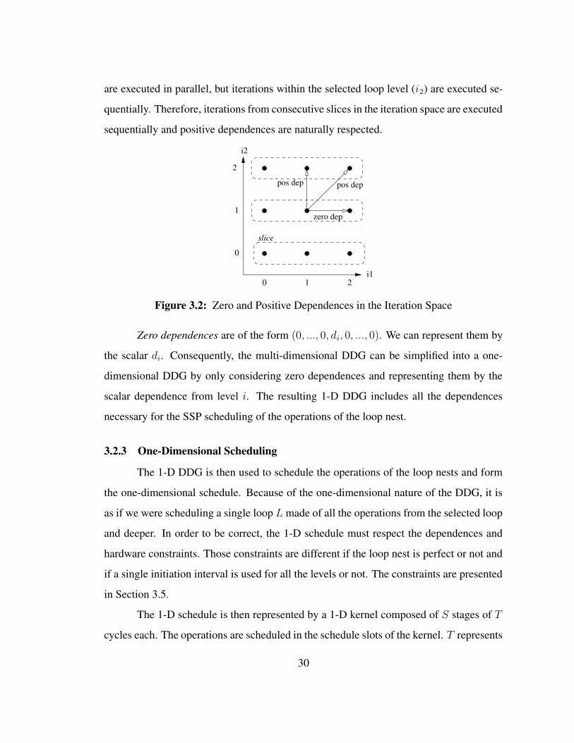
are executed in parallel, but iterations within the selected loop level (i2) are executed se-

quentially. Therefore, iterations from consecutive slices in the iteration space are executed

sequentially and positive dependences are naturally respected.

0 1 2

0

1

2

i2

i1

pos deppos dep

zero dep

slice

Figure 3.2: Zero and Positive Dependences in the Iteration Space

Zero dependences are of the form (0, ..., 0, di, 0, ..., 0). We can represent them by

the scalar di. Consequently, the multi-dimensional DDG can be simplified into a one-

dimensional DDG by only considering zero dependences and representing them by the

scalar dependence from level i. The resulting 1-D DDG includes all the dependences

necessary for the SSP scheduling of the operations of the loop nest.

3.2.3 One-Dimensional Scheduling

The 1-D DDG is then used to schedule the operations of the loop nests and form

the one-dimensional schedule. Because of the one-dimensional nature of the DDG, it is

as if we were scheduling a single loop L made of all the operations from the selected loop

and deeper. In order to be correct, the 1-D schedule must respect the dependences and

hardware constraints. Those constraints are different if the loop nest is perfect or not and

if a single initiation interval is used for all the levels or not. The constraints are presented

in Section 3.5.

The 1-D schedule is then represented by a 1-D kernel composed of S stages of T

cycles each. The operations are scheduled in the schedule slots of the kernel. T represents

30

L1: for i1 = 0, N1 − 1 doop1

L2: for i2 = 0, N2 − 1 doop2

op3

op4

end forend for

(a) Original Loop Nest

op1c b a

T=2

S1=3

S2=2

op2op3op4

(b) Kernel

Figure 3.3: Kernel Example

the initiation interval of the kernel, i.e. the number of cycles between each issue of a new

outermost iteration. The smaller the initiation interval is, the faster the entire schedule

will execute. Si designates the number of stages corresponding to loop Li. More than

one operation may be scheduled in a schedule slot. Within each row of the kernel, the

operations do not compete for the same hardware resource. Figure 3.3 shows an example

of a kernel for a double loop nest. Examples and more formal definition of the kernel are

presented in Section 3.4.

......

... ...

op1op2op3op4

op1op2op3op4

op1op2op3op4

kernel

i10 1 2 3 4

cycles

Figure 3.4: Kernel in the Final Schedule Example if N2 = 1

Traditionally the kernel corresponds to the steady phase of the software-pipelined

schedule in MS. We extend here the terminology to the SSP method. Intuitively the

31

columns in the kernel corresponds to consecutive outermost iterations and the final sched-

ule should be composed of successive instances of the kernel where a new outermost it-

eration is issued every T cycles. Figure 3.4 shows how the kernel may appear in the final

schedule if N2 = 1. Each column represents the execution of one outermost iteration i1.

If N2 > 1 however, the steady phase of the final schedule is not uniquely composed of

the kernel. For more details, the reader is referred to Section 3.4.

3.2.4 Multi-Dimensional Scheduling

The last step is to compute the final schedule. It is obtained by using the 1-D

schedule as a footprint and taking into account the limited hardware resources of the

target processor. An example is presented in Figure 3.5 using the kernel presented in

Figure 3.3. We assume that there are only 2 functional units available and that N2 = 3

and N1 = 4. Each column represents an outermost iteration. Innermost iterations are

grouped in slices, with a different shade of gray for each innermost iteration index value.

Ideally the final schedule issues a new outermost iteration every T cycles as shown

in Figure 3.5(a). The outermost iterations are executed in parallel, while the inner itera-

tions are executed sequentially within each outermost iteration. However, very quickly,

the number of operations to execute per cycle exceeds the capacity of the target architec-

ture and lead to resource conflicts.

In order to correctly execute the schedule, a delay is added to stall the execution of

some outermost iterations. The delay must allow the schedule to run with the functional

units available in the target processor and make repeating patterns appear to allow for

the compact code emission of the final schedule. In SSP, the delay operation is applied

to groups of Sn outermost iterations, where Sn is the number of stages in the kernel

containing operations from the innermost loop. If more than Sn iterations were to be

included in the same iteration group, then the instances of the same innermost stages

would be executed in parallel. That scenario was not considered while generating the

kernel and therefore could lead to some resource conflicts. In our example, Sn = 2 and

32

op1

op2op3

op4op2op3

op4

op4

op2op3

op1

op2op3

op4op2op3

op4

op4

op2op3

op1

op2op3

op4op2op3

op4

op4

op2op3

op1

op2op3

op4op2op3

op4

op4

op2op3

slice 0

slice 1(i2=1)

(i2=0)

slice 2(i2=2)

0 1 2 3

resource conflicts

T=2

cycles

i1

(a) Ideal Schedule

op1

op2op3

op4op2op3

op4

op4

op2op3

op1

op2op3

op4op2op3

op4

op4

op2op3

op1

op2op3

op4op2op3

op4

op4

op2op3

op1

op2op3

op4op2op3

op4

op4

op2op3

0 1 2 3

delay

cycles

i1

kernel

group 1group 0

(b) Final Schedule

Figure 3.5: Multi-Dimensional Scheduling Example

33

we obtain the conflict-free final schedule shown in Figure 3.5(b). Some repeating patterns

appear, like the full kernel for instance. More details about the patterns and final schedules

are given in Section 3.4.

3.2.5 Properties

SSP schedules have two interesting properties. First, if applied to the innermost

level of a loop nest, SSP is equivalent to MS. Indeed there is then no dependence simplifi-

cation and the scheduler becomes a traditional MS scheduler generating a traditional MS

kernel. Therefore SSP can be seen as the generalization of MS to loop nests. Since the

innermost level can always be selected, the performance of the SSP schedule can never

be below the performance of the MS schedule.

Second, for perfect loop nests, SSP schedules are proven to be shorter than MS

schedules in terms of static cycles. Indeed, SSP overlaps the prolog and epilog of the

innermost loop and manages to keep the processor busy during the entire execution of

the schedule. If the loop nest is a single loop, then the two schedules are equivalent.

The theorem and proof are described along the schedule function for perfect loop nests in

Section 3.6.1.

3.3 SSP Implementation

The actual implementation of the SSP method into a compiler consists of severals

steps that differ from the theoretical framework. Those steps, leading to the final assembly

code, are shown in Figure 3.6. The implementation of each of those steps is one of the

main contributions of this dissertation. The related details are presented in subsequent

chapters.

The first step is again the loop selection step. We assume that the compiler pro-

vides the SSP framework with a complete multi-dimensional DDG. It may require some

information propagation about the dependences as multi-dimensional dependences are

34

n−D DDG

loop nest

loop nest

loop level

(1−D schedule)

kernel

assembly code

(final schedule)

register−allocated kernel

1−D DDG register pressure oktoo highor

SelectionLoop

SimplificationDDG

GenerationKernel

GenerationCode

AllocationRegister

Register PressureEvaluation

Figure 3.6: The SSP Framework

usually computed early in the compilation process. Loop selection heuristics are pre-

sented in Chapter 4 and were published in [RTG+04].

Once the level is chosen, the multi-dimensional DDG is simplified into a one-

dimensional DDG as explained in the previous section. This work was published in

[RTG+04].

Using the 1-D DDG, a scheduler produces the 1-D schedule, represented by the

kernel. The 1-D schedule honors the dependences from the one-dimensional graph and

takes into account the number and properties of each functional unit described in sec-

tion 3.5. The scheduler is similar to a modulo scheduler but must take into account fea-

tures specific to the SSP method and the multi-dimensional nature of the problem such

multiple kernels or multiple initiation intervals. Several scheduling algorithms are pre-

sented in Chapter 5 and were published in [DRG06].

Once the 1-D schedule is obtained, the register pressure is quickly evaluated using

a method explained in Chapter 6 and published in [DG05]. If the register pressure is too

high, the scheduler or the loop selector are asked to come up with different choices leading

to a smaller register pressure. Registers are then allocated. The method considers the

features of the multi-dimensional vector lifetimes specific to the SSP case. The register

35

allocation method is presented in Chapter 7 and was published in [RDG05].

Finally the final schedule is generated in assembly code by the code generator.

Loop overheads and architectural specifics such as register rotation are also handled by

the code generator. An implementation is described in Chapter 8 and was published in

[RDGG04].

3.4 Examples & Notations

In this section, different examples are proposed to help understand the SSP sched-

ules. First, a comparison between SSP and MS showing the potential of the SSP method

is proposed. Then, two examples of complete SSP schedules are described. The first

example deals with a double loop nest. The second considers a more complex case with

a triple loop nest. The last subsection introduces the notations about kernels.

3.4.1 SSP vs. MS Example

To show the potential of the SSP method, let us consider the double loop nest

example shown in Figure 3.7. The original source code is shown in Figure 3.7(a). We as-

sume that its intermediate form after transformations and just before the SSP/MS schedul-

ing phase is as shown in Figure 3.7(b). For clarity reasons, each operation is referred to

as op1, op2, etc... n will always refer to the depth of the loop nest, outer loops to all the

loops but the innermost and inner loops to all the loops but the outermost.

We now assume that the heuristic used by the loop selector chose the outermost

loop for software-pipelining. The kernel generated by the scheduler is shown in Fig-

ure 3.8. It is a two-dimensional SSP kernel composed of 5 stages of 2 cycles each. To

obtain such a kernel, we assume that the target processor is composed of only 2 mem-

ory units, and that we have latencies of 1, 2, and 3 cycles for the +, load/store, and *

operations respectively. For MS, the kernel is simply the innermost kernel represented in

shadow-gray boxes. The two kernels are similar because SSP is equivalent to MS when

applied to the innermost loop. It is therefore correct that they share the same innermost

36

total = 0L1: for I = 1, 6 doL2: for J = 1, 3 do

B[J] = A[I] * B[J]end fortotal += B[3]

end for

(a) Source Code

L1: for I = 1, 6 doop1: t1 = load addr1, 4

L2: for J = 1, 3 doop2: t2 = load addr2op3: t3 = t1 * t2op4: store t3, addr2, 4

end forop5: t4 = t3 + t4

end for

(b) Intermediate Form

Figure 3.7: MS vs. SSP: Loop Nest

kernel. In order to later represent schedules in a compact way, the stages of the kernel are

named a, b,...etc

e abcdop3

op4op1op2

op5

Figure 3.8: MS vs. SSP: Kernel

The full MS schedule, derived from the MS kernel, is shown in Figure 3.9(a).

The stages are now represented by their letters and the operations within are hidden.

Each stage takes two cycles to execute. The gray boxes still represent the innermost

stages, i.e. containing the operations from the innermost loop. By definition of a modulo

schedule, the innermost operations are executed in parallel once the pipeline has been

filled. It is represented by the horizontal row of stages d, c, and b. However, the outermost

iterations are not executed in parallel, which leads to a poor processor busy ratio and a

total schedule time of 84 cycles. At best, if hierarchical reduction [Lam88] is applied

using Muthukumar’s technique [MD01], then the prolog phase of the innermost pipeline

can overlap the epilog phase of the innermost pipeline of the previous outermost iteration.

The result is shown in Figure 3.9(b). The schedule time is reduced to 54 cycles.

37

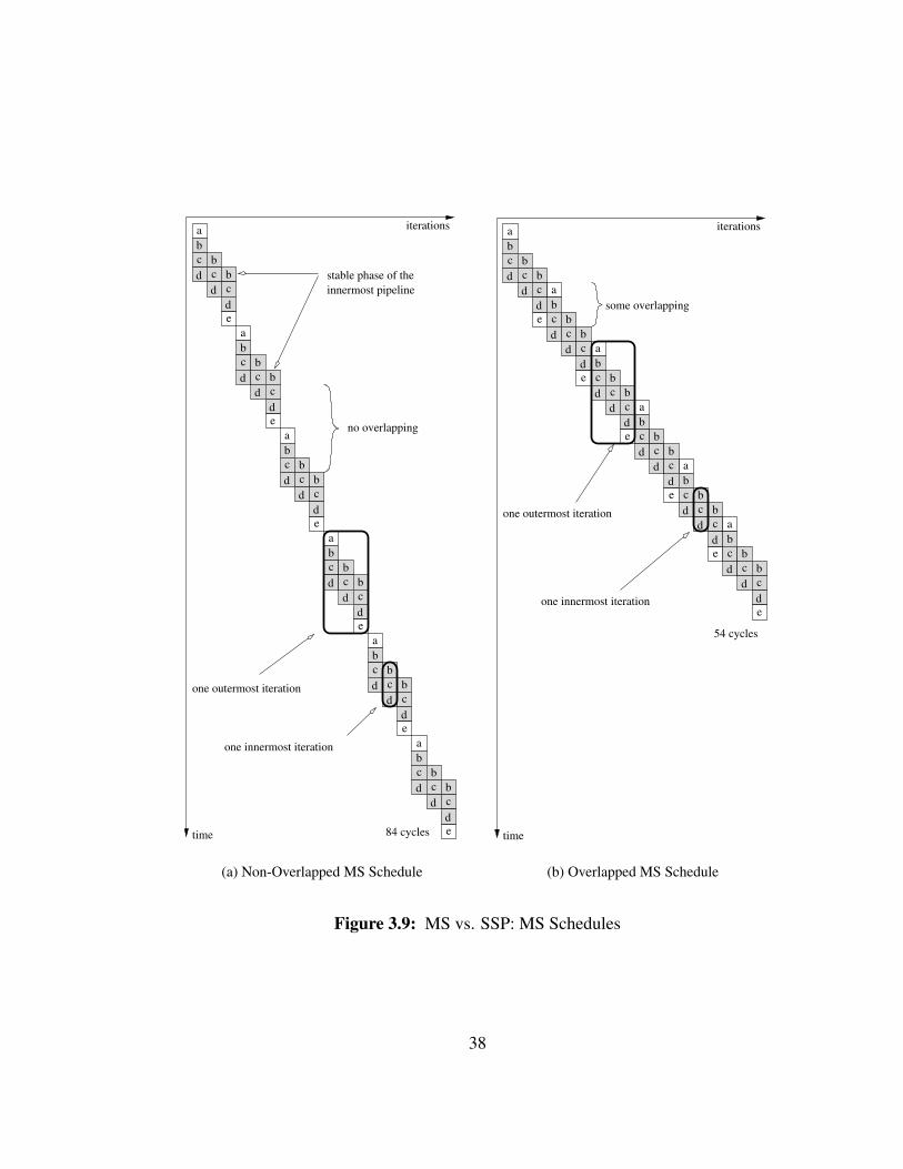
abcd

bcd

bcde

abcd

bcd

bcde

abcd

bcd

bcde

abcd

bcd

bcde

abcd

bcd

bcde

abcd

bcd

bcdetime

iterations

84 cycles

stable phase of theinnermost pipeline

no overlapping

one innermost iteration

one outermost iteration

(a) Non-Overlapped MS Schedule

abcd

bcd

bcde

abcd

bcd

bcde

abcd

bcd

bcde

abcd

bcd

bcde

abcd

bcd

bcde

abcd

bcd

bcde

iterations

time

54 cycles

some overlapping



(b) Overlapped MS Schedule

Figure 3.9: MS vs. SSP: MS Schedules

38

abcdbcdbcd

bcdbcdbcd

bcdbcdbcd

aa

aa

ae

ebcd

bcd

bcdb

cd

bcd

bcd

bcd

bcd

bcd

ee

ee

iterations

time 44 cycles



high overlapping

Figure 3.10: MS vs. SSP: SSP Schedule

However the SSP schedule is still shorter by 10 cycles. Indeed, the processor is

kept busy most of the time and all the stages are sometimes executed concurrently. This

example shows that, given the same resources and even the same instruction scheduler,

SSP schedules can be shorter than MS schedules. And since the innermost level of the

a loop nest can always be selected and SSP is equivalent to MS when applied to a sin-

gle loop, the maximum length of the SSP schedule is bounded by the length of the MS

schedule.

3.4.2 Double Loop Nest Example

To illustrate the different steps of the SSP framework, a double loop nest exam-

ple is proposed in Figure 3.11(a). The corresponding n-D DDG, is shown next to it in

Figure 3.11(b). The exact operations have been abstracted for clarity purposes.

The first step is to decide which loop level to software pipeline. We will assume

that the loop selector deemed loop level L2 as the most profitable according to the heuris-

tic used and that L2 has been selected for software-pipelining. The loop nest that we will

39

L1: for I = 1, 100 doop0

L2: for J = 1, 7 doop1

L3: for K = 1, 4 doop2op3op4

end forop5

end forend for

(a) Triple Loop Nest

op1

op4 op3

op5 op2op0

<0,1,0>

<0,0,0>

<0,0,1><0,0,0>

<0,0,0>

<0,0,0>

<0,1,0><1,0,0>

<0,1,0>

(b) Multi-Dimensional DDG

Figure 3.11: Double Loop Nest Example: Inputs

now consider is shown in Figure 3.12. Because the original outermost loop was discarded,

we will no longer refer to it. From the SSP framework point of view, the original L2 is now

the outermost loop level. Therefore the loops are renamed and L2 and L3 become the new

L1 and L2 respectively. Such renaming is always possible after loop selection. Therefore,

in the rest of the dissertation, we will always assume that the software-pipelined loop is

the outermost loop level of the loop nest.

L1: for I = 1, 7 doop1

L2: for J = 1, 4 doop2op3op4

end forop5

end for

Figure 3.12: Double Loop Nest Example: Loop Nest After Loop Selection

The next step is to simplify the n-D DDG into a 1-D DDG. Only the two innermost

40

dimensions of the n-D DDG are considered. Positive dependences are discarded. Zero

dependences are kept and the iteration distance of the selected loop level is used as the

iteration distance for the 1-D DDG. The resulting 1-D DDG is shown in Figure 3.13(a).

op1

op4 op3

op5 op2

1

0

0

0

0

1

(a) Simplified DDG

Number of All-purpose FUs: 2operation 0 1 2 3 4 5latency 2 2 2 1 1 2

(b) Resources

op1

op2op3

op4op5

abcd

T1T2

S1

S2

unused

(c) Kernel

Figure 3.13: Double Loop Nest Example: 1-D Schedule

Given the 1-D DDG and the resources of the target processor, shown in Fig-

ure 3.13(b), a 1-D schedule can be computed. The 1-D schedule is represented by a

kernel shown in Figure 3.13(c). The innermost stages have been grayed out. The op-

erations are scheduled so that the latencies between dependent operations are respected.

Also, at each given cycle, the number of scheduled operations never exceed the number of

available functional units (2). The kernel is composed of 2 outermost stages and S2 = 2

innermost stages for a total of S1 = 4 stages. The initiation interval of the outermost

kernel is equal to T1 = 3. However, the initiation interval of the innermost kernel, i.e. the

kernel used to generate the schedule corresponding to the execution of the innermost loop

and represented by the gray boxes, is lower and equal to T2 = 2. It is therefore a multiple

initiation interval kernel.

41

a

a

b

cc

cc

cc

b

b

bb

b

b

cc

cc

cc

b

b

bb

b

b

b

b

c

cd

a

a

b

b

c

cd

a

a

d

cc

cc

cc

b

b

bb

b

b

b

b

c

cd

ad

c

c

cb

b

b

cd

d 102 cycles

innermost iterations from

run concurrentlydifferent outermost iterations

outermost iteration

innermost iteration(runs sequentially with theother innermost iterationswithin the same outermostiteration)

time

(runs concurrently with theother outermost iterations)

1 outermostiterations

765432

1 2 3 4 scheduling groups

delay

T1=3

T2=2

Figure 3.14: Double Loop Nest Example: Final Schedule

42

The impact of multiple initiation interval kernel can be seen in the final schedule

shown in Figure 3.14. The stages are represented by their symbolic letters for readability

purposes. Small horizontal tics delimit the cycles within each stage. When an inner-

most stage is used alongside an outermost stage with a higher initiation interval, then its

initiation interval is adjusted with the schedule slots marked as ’unused’ in the kernel.

Otherwise, the innermost initiation interval of 2 is used. If the initiation interval of the

innermost kernel was always equal to T1 = 3 cycles, then the execution of the inner loops

would be delayed, and the final schedule would be 24 cycles longer in this particular

example.

The delay function used to enforce the resource constraints in the final schedule

has been represented by thick black arrows. Every stage that does not belong to an itera-

tion from the current group of outermost iterations is delayed. The start time of iterations

3 and above have been delayed accordingly in groups of Sn outermost iterations. Stage d

from the last outermost iteration of each scheduling group was also delayed.

The schedule illustrates how outermost iterations are executed in parallel whereas

the innermost iterations within the same outermost iteration are executed sequentially.

Innermost iterations from different outermost iterations, on the other hand, are also exe-

cuted in parallel. Because the number of outermost iterations is not a multiple of Sn, the

last outermost iteration is executed alone.

It is worth noting that the positive dependence from op4 to op2 in the original n-D

DDG is still respected. Indeed, op2 from innermost iteration J is always executed at least

1 cycle after op4 from innermost iteration J − 1.

3.4.3 Triple Loop Nest Example

The next example shows how the final schedule differs when the loop nest contains

three loops or more. The section of the schedule during the delay now also includes

the middle loops which leads to more complex patterns and a more complex schedule

43

function. The duration of the delay is also increased to take into account the newly added

loops.

We assume that the multiple initiation interval kernel of a triple loop nest is as

shown in Figure 3.15. Again, the innermost stages are grayed out while the unused sched-

ule slots are shown with hashes. The middle kernel, i.e. the kernel corresponding to the

middle loop of the original loop nest, is composed of S2 = 4 stages b, c, d, and e. As op-

posed to the previous example, the inner kernels, innermost and middle, are not scheduled

in the last schedule rows of the outermost kernel.

op6

op7

op8

op9

ef

T3

S3

op1

op2

op3

op4

op5

abcd

T2

S2

S1

T1

Figure 3.15: Triple Loop Nest Example: Kernel

The final schedule corresponding to the proposed kernel is shown in Figure 3.15.

We assume that the number of iterations for the loops are 8, 2, and 3, from the outermost

to the innermost level respectively. Indeed we have 8 columns corresponding to the 8

outermost iterations. Within each outermost iteration, the stages b and e appear only

twice, and between each appearances, the innermost stages c and d are executed three

times. Unlike the double nest example, stages are not represented in the figure according

to their to their initiation interval of the stages for space reasons.

This time the schedule has been decomposed into different sections that will later

useful for the code generation phase. The schedule starts with a Prolog, only composed

of stage a in this example. Then it is an alternation of two segments: the Outermost Loop

Pattern (OLP) and the Inner Loop Execution Segments (ILES). OLP corresponds to the

part of the schedule where outermost stages are executed. The ILES corresponds to the

44

time

a

aa

bbc

ccd

dc

cd

d

debc

cd

be

ccd

dc

cd

d

b ac b

d ce d

eff

d ce d

eff

eff

d c b ae d c b a

d c b ae d c b a

eff

Innermost LoopPattern (ILP)

Draining & FillingPattern (DFP)


Outermost LoopPattern (OLP)

Segment (ILES)Innermost Loop Execution


1 765432

1 32 4

8

scheduling groups

Epilog

Folded ILES

Prologoutermostiterations

Figure 3.16: Triple Loop Nest Example: Schedule

45

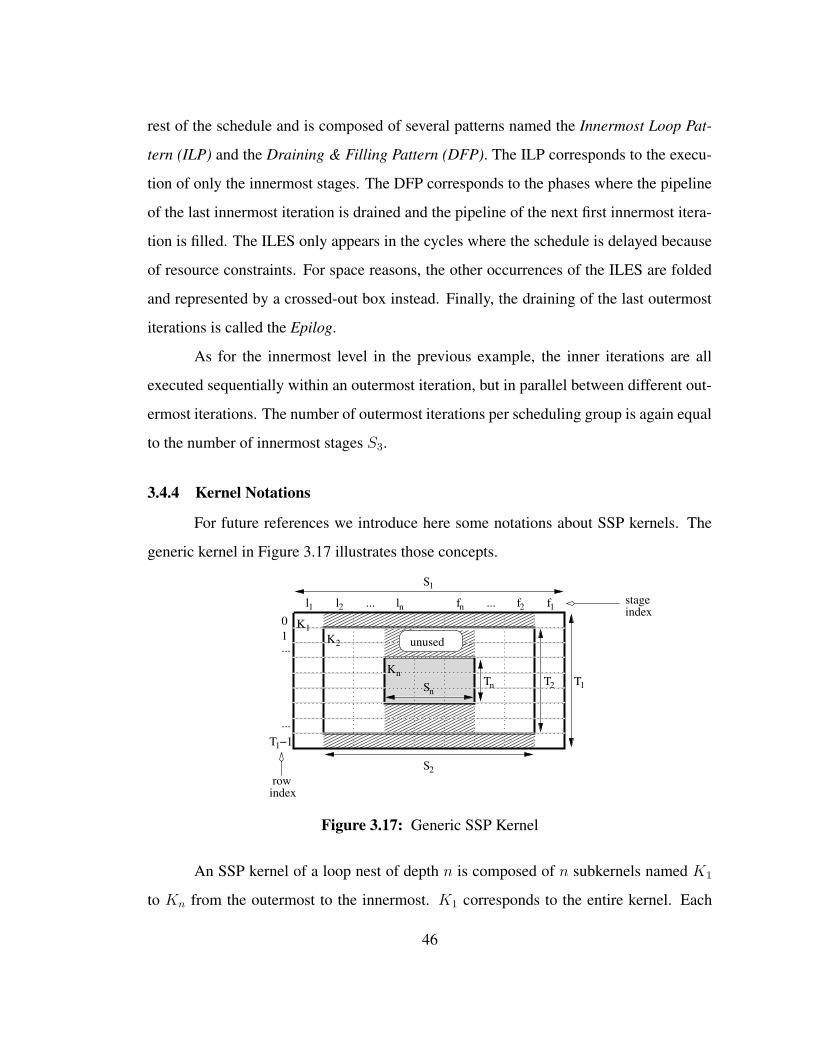
rest of the schedule and is composed of several patterns named the Innermost Loop Pat-

tern (ILP) and the Draining & Filling Pattern (DFP). The ILP corresponds to the execu-

tion of only the innermost stages. The DFP corresponds to the phases where the pipeline

of the last innermost iteration is drained and the pipeline of the next first innermost itera-

tion is filled. The ILES only appears in the cycles where the schedule is delayed because

of resource constraints. For space reasons, the other occurrences of the ILES are folded

and represented by a crossed-out box instead. Finally, the draining of the last outermost

iterations is called the Epilog.

As for the innermost level in the previous example, the inner iterations are all

executed sequentially within an outermost iteration, but in parallel between different out-

ermost iterations. The number of outermost iterations per scheduling group is again equal

to the number of innermost stages S3.

3.4.4 Kernel Notations

For future references we introduce here some notations about SSP kernels. The

generic kernel in Figure 3.17 illustrates those concepts.

unused

f2 f1

T2 T1nTKn

K2

K1

S2

Sn

fnlnl2l1

S1

T −11

stageindex

......01...

...

rowindex

Figure 3.17: Generic SSP Kernel

An SSP kernel of a loop nest of depth n is composed of n subkernels named K1

to Kn from the outermost to the innermost. K1 corresponds to the entire kernel. Each

46

subkernel Ki is made of Si = li− fi stages where fi and li are the indexes of the first and

last stage of Ki in K1. The initiation interval of each subkernel Ki is noted Ti. The used

schedule slots may contain 0, 1, or more operations. The number of operations within one

cycle, i.e. a row in the generic kernel, is limited by the resource constraints. The number

of unused cycles above subkernel Ki is noted Tai. The number of unused cycles below

subkernel Ki is noted Tbi.

The 1-D schedule function of an operation op in the kernel is noted σ(op, i1). i1

represents the outermost iteration index. Operations from the same instance of the kernel

share the same i1 value. The stage index and row index can be derived from the 1-D

schedule function. We can write σ(op, 0) = p ∗ T + q where q < T . Then p is the stage

index of op and q the row index of op in the kernel. We also have p = bσ(op, i1)/T cand q = σ(op, i1) modulo T . The stage and row indexes will be necessary for several

algorithms in subsequent chapters.

If the loop nest is perfect, the kernel is composed solely of the innermost kernel

Kn. Therefore a single initiation interval T = Tn is used. In the most general case, the

loop nest is imperfect and each loop level uses its own initiation interval. For theoretical

and practical issues, a kernel with multiple initiation interval can always be considered

as a schedule with single initiation interval from which the unused cycles have been re-

moved.

For clarity reasons, the unused slots of the subkernels are assumed to contain no

operations. However, the theory and algorithms presented in the dissertation consider

that operations may appear in those cycles. Indeed an operation from level i can appear

in any cycle within the boundaries of subkernel Ki. Some practical issues will limit such

freedom at the code generation level, as presented in Chapter 8.

3.5 One-Dimensional Schedule Constraints

The 1-D schedule must obey some constraints to be correct. This section presents

those constraints in three situations from the most specific to the most general: perfect

47

loop nests, imperfect loop nests with single initiation interval, and imperfect loop nests

with multiple initiation intervals.

3.5.1 Perfect Loop Nests

In the case of perfect loop nests, the 1-D schedule is uniquely composed of opera-

tions from the innermost loop. Therefore the kernel consists of only innermost stages and

all the stages have the same initiation interval T . The constraints to be respected by the

1-D schedule can then be written as shown in Figure 3.18.

• Modulo Property:

σ(op, i1 + 1) = σ(op, i1) + T (3.1)

• Dependence Constraints:

σ(op1, i1) + δ ≤ σ(op2, i1 + k) (3.2)

for all the dependences from the 1-D DDG from op1 to op2 where δ is thelatency of the dependence and k the distance.

• Resource Constraints:

At any given cycle of the 1-D schedule, a hardware resource is not allocatedto more than one operation.

• Sequential Constraints:

σ(op, 0) + δmax(op) ≤ S ∗ T (3.3)

where δmax(op) = max(δ) for all the positive dependences starting from opin the original n-D DDG.

Figure 3.18: 1-D Schedule Constraints in the case of Perfect Loop Nests

The first 3 constraints are the same as the constraints used in MS. The modulo

constraint ensures that a new outermost iteration is issued every T cycles. The dependence

constraint ensures that the dependences from the 1-D DDG are respected while taking into

48

account the modulo property. The resource constraints ensures that the target architecture

can actually execute the 1-D schedule.

The sequential constraint however is unique to the SSP method. It ensures that the

positive dependences, not present in the 1-D DDG, are respected. In the final schedule,

such a dependence only exist between operations from different slices (Figure 3.2). If the

dependence is already respected at the end of the slice of the originating operation, then it

will be guaranteed to be respected in the subsequent slices. In the first outermost iteration

of the first slice, as shown in Figure 3.19, the destination operation can be scheduled once

the positive dependence is respected, i.e. after cycle σ(op, 0) + δmax. The end of the

first slice is at cycle S ∗ T , where S ∗ T is the length of the 1-D schedule (S stages of T

cycles each). Therefore the positive dependence is always respected if we guarantee that

σ(op, 0) + δmax(op) ≤ S ∗ T . Because the destination operation is not necessarily in the

first cycle of the next slice, the constraint is not tight. However it simplifies the schedul-

ing process while making sure that positive dependences are respected. In practice, the

constraint is respected most of the time without taking any special action.

abcdabcdabcd

abcd

abcd

abcd

abcd

abcd

abcd

abcd

abcd

abcd

abcd

abcd

abcd

slice 0

slice 1

slice 2

positive dependence

S.T

σ

δ

Figure 3.19: Sequential Constraint Example

49

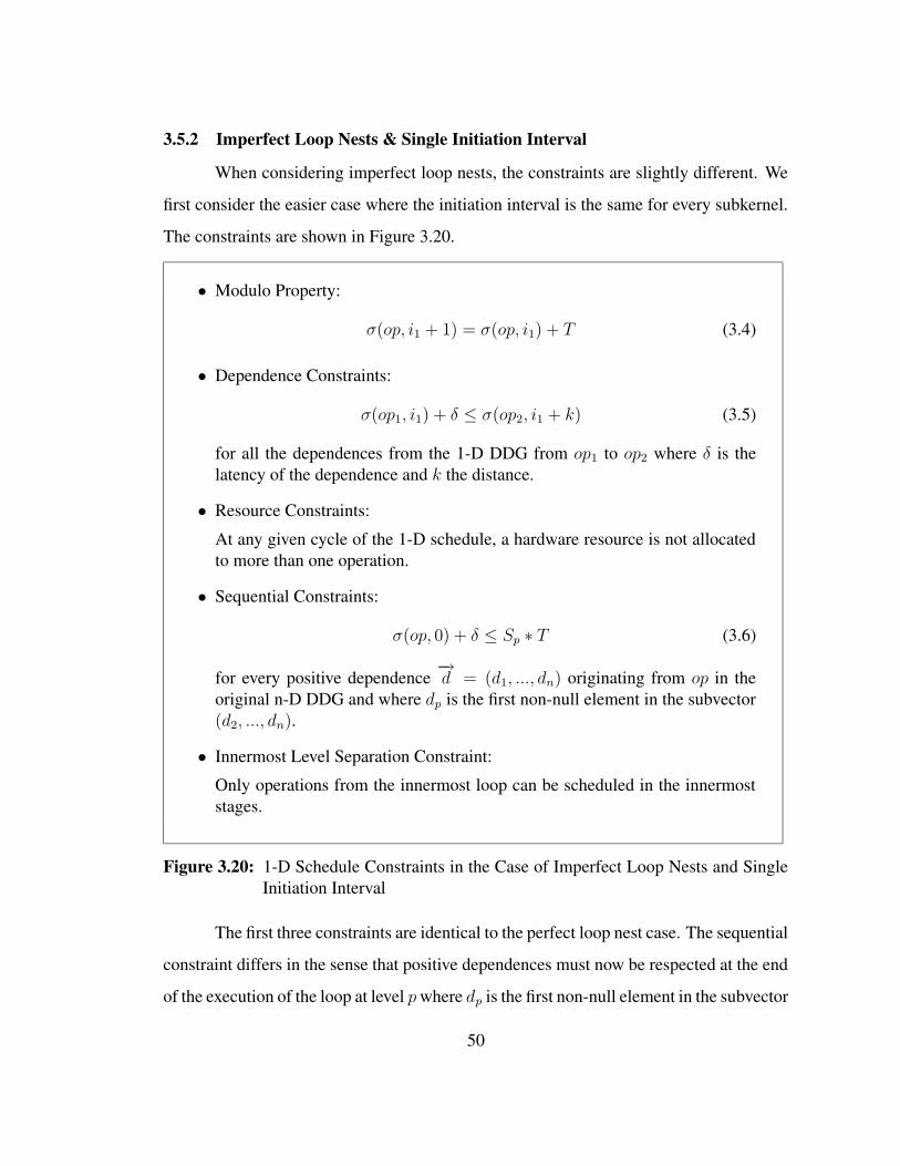
3.5.2 Imperfect Loop Nests & Single Initiation Interval

When considering imperfect loop nests, the constraints are slightly different. We

first consider the easier case where the initiation interval is the same for every subkernel.

The constraints are shown in Figure 3.20.


σ(op, i1 + 1) = σ(op, i1) + T (3.4)


σ(op1, i1) + δ ≤ σ(op2, i1 + k) (3.5)





σ(op, 0) + δ ≤ Sp ∗ T (3.6)

for every positive dependence−→d = (d1, ..., dn) originating from op in the

original n-D DDG and where dp is the first non-null element in the subvector(d2, ..., dn).

• Innermost Level Separation Constraint:

Only operations from the innermost loop can be scheduled in the innermoststages.

Figure 3.20: 1-D Schedule Constraints in the Case of Imperfect Loop Nests and SingleInitiation Interval

The first three constraints are identical to the perfect loop nest case. The sequential

constraint differs in the sense that positive dependences must now be respected at the end

of the execution of the loop at level pwhere dp is the first non-null element in the subvector

50

(d2, ..., dn). The size of corresponding slice is therefore Sp ∗ T instead of S ∗ T . Because

p may be different for each positive dependence originating from the same operation, the

latency δ is used instead of δmax.

The last constraint is new and not necessary in theory. In practice, however, it is

required to limit the code size of the final schedule during the code generation step. A 1-D

schedule that does not respect the innermost level separation constraint would be correct,

but too inefficient to use in practice. For more details, the reader is referred to Chapter 8.

3.5.3 Imperfect Loop Nests & Multiple Initiation Intervals

If multiple initiation intervals are allowed in the kernel, then the constraints are

different, as shown in Figure 3.21.

The modulo property and the resource and innermost level separation constraints

are unchanged. The separation constraint is considering the worst-case scenario in the

sense that it becomes more complex to compute the length of the execution of loop level

p. The smallest initiation interval is Tn so a lower bound of the length of the execution of

loop level p is Sp ∗ Tn.

The dependence constraint must now take into account the missing cycles oc-

curred by the multiple initiation interval situation. The function that returns the num-

ber of missing cycles between the schedule cycles of operations op1 and op2 is named

UnusedCycles(op1, op2, k). If p1 and p2 are the stage indexes of op1 and op2 respec-

tively, and if level(s) returns the level of stage s, then the function is defined as:

If σ(op1, 0) ≤ σ(op2, 0) and p1 = p2, then

UnusedCycles(op1, op2, k) = k ∗s=S−1∑

s=0

(T − Tlevel(s)) (3.10)

51


σ(op, i1 + 1) = σ(op, i1) + T (3.7)


σ(op1, i1) + δ ≤ σ(op2, i1 + k)− UnusedCycles(op1, op2, k) (3.8)





σ(op, 0) + δ ≤ Sp ∗ Tn (3.9)





Figure 3.21: 1-D Schedule Constraints in the Case of Imperfect Loop Nests and MultipleInitiation Intervals

52

If σ(op1, 0) ≤ σ(op2, 0) and p1 < p2, then

UnusedCycles(op1, op2, k) =

s=p2−1∑

s=p1+1

(T − Tlevel(s)) + Tblevel(p2) + Talevel(p1)

+k ∗s=S−1∑

s=0

(T − Tlevel(s)) (3.11)

Otherwise, if σ(op1, 0) > σ(op2, 0), the function is defined as:

UnusedCycles(op1, op2, k) =s=S−1∑

s=p1+1

(T − Tlevel(s)) +

s=p2−1∑

s=0

(T − Tlevel(s))

+Tblevel(p2) + Talevel(p1)

+k ∗s=S−1∑

s=0

(T − Tlevel(s)) (3.12)

The number of missing cycles is obtained by counting all the unused cycles between

op1 and op2. That number includes the unused cycles of the stages between the two

operations, stages of the operations excluded, the unused cycles in the stage of op2 before

op2 (Tblevel(p2)), the unused cycles in the stage of op1 after op1 (Talevel(p1)), and the total

number of unused cycles in the kernel multiplied by the distance k. Depending on the

relative 1-D schedule time of the two operations, the unused cycles of the stages between

the two operations differ. Figure 3.22 illustrates it with a kernel example from a 3-deep

loop nest. The thick black strip represents the distance between the two operations while

the unused cycles that need to be subtracted from that distance have been grayed out. The

terms corresponding to the sum(s) in UnusedCycles have been noted with a large sigma

sign, and the others with Ta and Tb.

The innermost level separation constraint does not prevent operations from level

i and below from appearing in the unused cycles of above and below subkernel Ki+1.

Those operations will be conditionally emitted to produce the final schedule, as explained

in Chapter 8. They do not interfere with the other constraints and the definition of

UnusedCycles.

53

op2

op1

Σ TaTb

(a) When σ(op1, i1) ≤ σ(op2, i1)

op2

op1

TbTaΣ Σ1 2

(b) When σ(op1, i1) > σ(op2, i1)

Figure 3.22: Unused Cycles Computation Examples

3.6 Schedule Function

We now present mathematical formulations of the schedule function of operations

in the final schedule when possible. Correctness proofs will also be given. We first present

the simpler case of perfect loop nests, followed by imperfect loop nests, with single, then

multiple initiation intervals.

3.6.1 Perfect Loop Nests

The final schedule cycle of an operation op at iteration−→I = (i1, ..., in) in a perfect

loop nest can be computed. To ease the understanding, Figure 3.23 shows an example of a

triple loop nest schedule. Because the loop nest is perfect, the kernel is composed of only

innermost stages and every stage has the same initiation interval T . The number of stages

is assumed to be equal to S = 2. One full innermost iteration is represented by a box.

The color of the box indicates the innermost iteration index within one middle iteration.

The darker the box, the greater the index. The number of iterations for each loop level

is N1 = 6, N2 = 2, and N3 = 2 from the outermost to the innermost respectively. The

dashed print represent the position of the outermost iterations before resource constraints

forced the iterations to be pushed down in the schedule.

The schedule function is composed of four terms. Each term is illustrated in the

Figure for an operation op from iteration (5, 1, 1). The first term gives the starting cycle

54

delay from outermostiteration index

delay from resourceconstraints

delay from inneriteration indexes

1−D schedule

time

outermostiterations

0 1 2 3 4 5

one middleiteration

iterationone innermost

operation o atindex (5,1,1)

Figure 3.23: Perfect Loop Nest: Schedule Example of Operation op at iteration index(5, 1, 1)

55

of an outermost iteration without resource constraints. Because in those conditions a new

outermost iterations is to be issued every T cycles, that term is equal to:

i1 ∗ T (3.13)

The second term takes into consideration the delay induced by the resource con-

straints. The execution of the stalled outermost iterations last for the entire execution of

the inner loops minus one innermost iteration which is executed in parallel with the other

outermost iterations. To execute all the inner iterations, each stage must be executed

N2 ∗N3. To execute all the stages once, it takes S ∗ T cycles. The delay S ∗ T ∗N2 ∗N3

must be applied every time, the outermost iteration is pushed down, i.e. bi1/Sc. There-

fore, in general, the delay from resource constraints is equal to:

S ∗ T ∗⌊i1S

⌋∗(j=n∏

j=2

Nj − 1

)(3.14)

The third term corresponds to the iteration of the instance of the operation within

the outermost iteration. In our example, i2 = 1 and i3 = 1, which means that the middle

loop must be fully executed once (i2 ∗ S ∗ T ∗N3 cycles) and that the innermost iteration

has already been executed once (i3 ∗ S ∗ T cycles). In the general case the corresponding

delay can be expressed as:

S ∗ T ∗k=n∑

k=2

(ik ∗

j=n+1∏

j=k+1

Nj

)where Nn+1 = 1 (3.15)

Finally, once the correct set of innermost stages has been reached, one only needs

to add the schedule cycle of operation op in the 1-D schedule, i.e. σ(op, 0). The final

schedule function f of an operation op at iteration index−→I = (i1, . . . , in) is then defined

as shown in Figure 3.24. It is correct as stated by the following theorem:

Theorem 3.1 If the loop nest is perfect, then the schedule function proposed in Equa-

tion 3.16 respects both the dependencies from the n-D DDG and the resource constraints

56

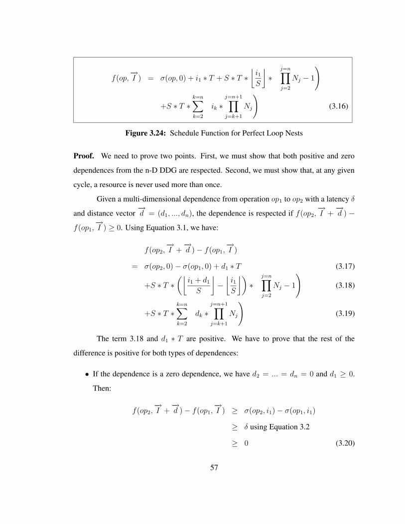
f(op,−→I ) = σ(op, 0) + i1 ∗ T + S ∗ T ∗

⌊i1S

⌋∗(j=n∏

j=2

Nj − 1

)

+S ∗ T ∗k=n∑

k=2

(ik ∗

j=n+1∏

j=k+1

Nj

)(3.16)

Figure 3.24: Schedule Function for Perfect Loop Nests

Proof. We need to prove two points. First, we must show that both positive and zero

dependences from the n-D DDG are respected. Second, we must show that, at any given

cycle, a resource is never used more than once.

Given a multi-dimensional dependence from operation op1 to op2 with a latency δ

and distance vector−→d = (d1, ..., dn), the dependence is respected if f(op2,

−→I +

−→d ) −

f(op1,−→I ) ≥ 0. Using Equation 3.1, we have:

f(op2,−→I +−→d )− f(op1,

−→I )

= σ(op2, 0)− σ(op1, 0) + d1 ∗ T (3.17)

+S ∗ T ∗(⌊

i1 + d1

S

⌋−⌊i1S

⌋)∗(j=n∏

j=2

Nj − 1

)(3.18)

+S ∗ T ∗k=n∑

k=2

(dk ∗

j=n+1∏

j=k+1

Nj

)(3.19)

The term 3.18 and d1 ∗ T are positive. We have to prove that the rest of the

difference is positive for both types of dependences:

• If the dependence is a zero dependence, we have d2 = ... = dn = 0 and d1 ≥ 0.

Then:

f(op2,−→I +−→d )− f(op1,

−→I ) ≥ σ(op2, i1)− σ(op1, i1)

≥ δ using Equation 3.2

≥ 0 (3.20)

57

• If the dependence is a positive dependence, we have σ(op2, i1) ≥ 0 by definition,

and, thanks to Equation 3.3,−σ(op1, i1) ≥ δmax(op1)−S∗T ≥ −S∗T . Therefore:

f(op2,−→I +−→d )− f(op1,

−→I ) ≥ −S ∗ T + S ∗ T ∗

k=n∑

k=2

(dk ∗

j=n+1∏

j=k+1

Nj

)

≥ S ∗ T ∗[k=n∑

k=2

(dk ∗

j=n+1∏

j=k+1

Nj

)− 1

](3.21)

If dp is the first non-null index of the positive dependence vector, then dp ≥ 1 and

we have:

k=n∑

k=2

(dk ∗

j=n+1∏

j=k+1

Nj

)

= dp ∗j=n+1∏

j=p+1

Nj +k=n∑

k=p+1

(dk ∗

j=n+1∏

j=k+1

Nj

)

≥ dp ∗j=n+1∏

j=p+1

Nj −k=n∑

k=p+1

(|dk| ∗

j=n+1∏

j=k+1

Nj

)because dk ≥ −|dk|

≥ dp ∗j=n+1∏

j=p+1

Nj +k=n∑

k=p+1

((1−Nk) ∗

j=n+1∏

j=k+1

Nj

)because |di| ≤ Ni − 1

≥ dp ∗j=n+1∏

j=p+1

Nj +k=n∑

k=p+1

j=n+1∏

j=k+1

Nj −k=n∑

k=p+1

(Nk ∗

j=n+1∏

j=k+1

Nj

)

≥ dp ∗j=n+1∏

j=p+1

Nj +k=n∑

k=p+1

j=n+1∏

j=k+1

Nj −k=n−1∑

k=p

j=n+1∏

j=k+1

Nj

≥ dp ∗j=n+1∏

j=p+1

Nj +Nn+1 −j=n+1∏

j=p+1

Nj

≥ (dp − 1) ∗j=n+1∏

j=p+1

Nj +Nn+1

≥ Nn+1 because dp ≥ 1

≥ 1 (3.22)

58

Therefore, using Equations 3.21 and 3.22, we can conclude that, in the case of a

positive dependence from op1 to op2, we have:

f(op2,−→I +−→d )− f(op1,

−→I ) ≥ 0 (3.23)

Using Equation 3.23 and Equation 3.20, we prove that both positive and zero depen-

dences, i.e. all the dependences from the original n-D DDG, are enforced.

Lastly, we need to prove that, at any cycle, no resource is used more than once.

Let op1 and op2 be two operations appearing in the same cycle in the final schedule at

iteration−→I = (i1, ..., in) and

−→I +−→d = (i1 +d1, ..., in+dn), respectively. Then we have:

f(op2,−→I +−→d )− f(op1,

−→I )

= σ(op2, i1)− σ(op1, i1) + d1 ∗ T + S ∗ T ∗k=n∑

k=2

(dk ∗

j=n+1∏

j=k+1

Nj

)

+S ∗ T ∗(⌊

i1 + d1

S

⌋−⌊i1S

⌋)∗(j=n∏

j=2

Nj − 1

)

= 0 (3.24)

If (d1, ..., dn) = (0, ..., 0), then σ(op1, i1) = σ(op2, i1). In other words, the two

operations belong to the same schedule slot of the kernel. Thanks to the resource con-

straint of the kernel, there cannot be any resource conflict between them. Therefore, if

there is a resource conflict, we must have (d1, ..., dn) 6= (0, ..., 0).

Because every term of the above equation, except σ(op2, i1) − σ(op1, i1), is a

multiple of T , then σ(op1, i1) and σ(op2, i1) have the same value modulo T . Therefore, if

there is a resource conflict, the two operations must appear in the same row in the kernel.

However, the resource constraint enforced on the kernel ensures that operations

scheduled in the same row have no resource conflict. Therefore, if there is a resource

conflict in the final schedule, at least one operation must have two instances scheduled at

the same cycle. If we can guarantee that at any cycle an operation appears no more than

once, then the schedule has no resource conflict.

59

Let us assume the contrary and prove that it is absurd. Let us assume that op1 =

op2. We have two cases depending on if the instances of the operation belong to the same

scheduling group or not:

• If the two instances of the operations belong to the same scheduling group, i.e. |d1|< S and

⌊i1S

⌋=⌊i1+d1

S

⌋, then we have:

f(op2,−→I +−→d )− f(op1,

−→I ) = 0

⇒ d1 ∗ T + S ∗ T ∗k=n∑

k=2

(dk ∗

j=n+1∏

j=k+1

Nj

)= 0

⇒ S ∗k=n∑

k=2

(dk ∗

j=n+1∏

j=k+1

Nj

)= −d1 (3.25)

⇒ S ∗∣∣∣∣∣k=n∑

k=2

(dk ∗

j=n+1∏

j=k+1

Nj

)∣∣∣∣∣ < S because |d1| < S

⇒∣∣∣∣∣k=n∑

k=2

(dk ∗

j=n+1∏

j=k+1

Nj

)∣∣∣∣∣ < 1

⇒k=n∑

k=2

(dk ∗

j=n+1∏

j=k+1

Nj

)= 0

We now prove by recurrence that the last equation implies that d2 to dn are equal

to zero. If n = 2, the property is obviously true. If the property is true for n = p,

i.e. we have the following recurrence property:k=p∑

k=2

(dk ∗

j=p+1∏

j=k+1

Nj

)= 0 =⇒ (d2, ..., dp) = (0, ..., 0)

we show that it is true if n = p+ 1:k=n∑

k=2

(dk ∗

j=n+1∏

j=k+1

Nj

)= 0

⇒ dn = −Nn ∗k=p∑

k=2

(dk ∗

j=p+1∏

j=k+1

Nj

)

⇒ |dn| = Nn ∗∣∣∣∣∣

k=p∑

k=2

(dk ∗

j=p+1∏

j=k+1

Nj

)∣∣∣∣∣

60

If the sum on the right-hand side is strictly positive, then |dn| > Nn, which is

impossible. Therefore the sum is equal to zero and dn = 0. Using the recurrence

property for n = p, we show that (d2, ..., dn − 1) = (0, ..., 0). Therefore our

recurrence property is also verified for n = p+ 1.

Thus, (d2, ..., dn) = (0, ..., 0). According to Equation 3.25, d1 is also equal to zero,

which is impossible because−→d 6= −→0 . Therefore op1 6= op2.

• If the two instances of the operations do not belong to the same scheduling group,

i.e.⌊i1+d1

S

⌋−⌊i1S

⌋≥ 1, then we have:

f(op2,−→I +−→d )− f(op1,

−→I )

≥ d1 ∗ T + S ∗ T ∗k=n∑

k=2

(dk ∗

j=n+1∏

j=k+1

Nj

)+ S ∗ T ∗

(j=n∏

j=2

Nj − 1

)

≥ d1 ∗ T − S ∗ T ∗k=n∑

k=2

(|dk| ∗

j=n+1∏

j=k+1

Nj

)+ S ∗ T ∗

(j=n∏

j=2

Nj − 1

)

Because |dk| ≤ Nk − 1, we can continue using Nn+1 = 1 later:

≥ d1 ∗ T + S ∗ T ∗[(

j=n∏

j=2

Nj − 1

)−

k=n∑

k=2

((Nk − 1) ∗

j=n+1∏

j=k+1

Nj

)]

≥ d1 ∗ T + S ∗ T ∗[j=n∏

j=2

Nj − 1−k=n∑

k=2

j=n+1∏

j=k

Nj +k=n∑

k=2

j=n+1∏

j=k+1

Nj

]

≥ d1 ∗ T + S ∗ T ∗[j=n+1∏

j=2

Nj − 1−k=n∑

k=2

j=n+1∏

j=k

Nj +k=n∑

k=2

j=n+1∏

j=k+1

Nj

]

≥ d1 ∗ T + S ∗ T ∗[j=n+1∏

j=2

Nj − 1−k=n−1∑

k=1

j=n+1∏

j=k+1

Nj +k=n∑

k=2

j=n+1∏

j=k+1

Nj

]

≥ d1 ∗ T + S ∗ T ∗[j=n+1∏

j=2

Nj − 1−j=n+1∏

j=2

Nj +Nn+1

]

≥ d1 ∗ T

Because f(op2,−→I +

−→d ) − f(op1,

−→I ) = 0 and T > 0, we have d1 = 0. However

we had by hypothesis d1 > 0. Therefore the result is absurd and op1 6= op2.

61

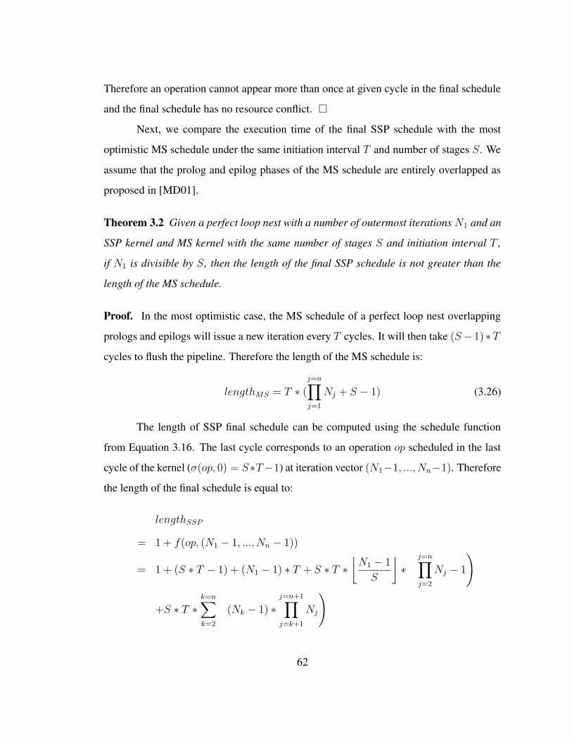
Therefore an operation cannot appear more than once at given cycle in the final schedule

and the final schedule has no resource conflict. �Next, we compare the execution time of the final SSP schedule with the most

optimistic MS schedule under the same initiation interval T and number of stages S. We

assume that the prolog and epilog phases of the MS schedule are entirely overlapped as

proposed in [MD01].

Theorem 3.2 Given a perfect loop nest with a number of outermost iterations N1 and an

SSP kernel and MS kernel with the same number of stages S and initiation interval T ,

if N1 is divisible by S, then the length of the final SSP schedule is not greater than the

length of the MS schedule.

Proof. In the most optimistic case, the MS schedule of a perfect loop nest overlapping

prologs and epilogs will issue a new iteration every T cycles. It will then take (S− 1) ∗Tcycles to flush the pipeline. Therefore the length of the MS schedule is:

lengthMS = T ∗ (

j=n∏

j=1

Nj + S − 1) (3.26)

The length of SSP final schedule can be computed using the schedule function

from Equation 3.16. The last cycle corresponds to an operation op scheduled in the last

cycle of the kernel (σ(op, 0) = S∗T−1) at iteration vector (N1−1, ..., Nn−1). Therefore

the length of the final schedule is equal to:

lengthSSP

= 1 + f(op, (N1 − 1, ..., Nn − 1))

= 1 + (S ∗ T − 1) + (N1 − 1) ∗ T + S ∗ T ∗⌊N1 − 1

S

⌋∗(j=n∏

j=2

Nj − 1

)

+S ∗ T ∗k=n∑

k=2

((Nk − 1) ∗

j=n+1∏

j=k+1

Nj

)

62

Because N1 is divisible by S,⌊N1−1S

⌋= N1

S− 1 and after expanding, we obtain:

= S ∗ T + (N1 − 1) ∗ T + S ∗ T ∗(N − 1

S− 1

)∗(j=n∏

j=2

Nj − 1

)

+S ∗ T ∗(k=n∑

k=2

j=n+1∏

j=k

Nj −k=n∑

k=2

j=n+1∏

j=k+1

Nj

)

= S ∗ T + (N1 − 1) ∗ T + S ∗ T ∗(N − 1

S− 1

)∗(j=n∏

j=2

Nj − 1

)

+S ∗ T ∗(k=n−1∑

k=1

j=n+1∏

j=k+1

Nj −k=n∑

k=2

j=n+1∏

j=k+1

Nj

)

= S ∗ T + (N1 − 1) ∗ T + S ∗ T ∗(N − 1

S− 1

)∗(j=n+1∏

j=2

Nj − 1

)

+S ∗ T ∗(j=n+1∏

j=2

Nj − 1

)by elimination and because Nn+1 = 1

= S ∗ T + (N1 − 1) ∗ T + S ∗ T ∗(N1 − 1

S

)∗(j=n+1∏

j=2

Nj − 1

)

= T ∗[S +N1 − 1 + (N1 − 1) ∗

(j=n+1∏

j=2

Nj − 1

)]

= T ∗[S +N1 − 1 +

j=n+1∏

j=1

Nj −N1

]

Therefore, we have:

lengthSSP = T ∗(S − 1 +

j=n+1∏

j=1

Nj

)(3.27)

Because Nn+1 = 1, Equations 3.26 and 3.27 are identical. Therefore, under the same

conditions, if N1 is divisible by S, then the SSP final schedule is at least as short as the

MS schedule. �If N1 is not divisible by S, loop peeling is always possible. Moreover, the extra

iterations are negligible compared to the execution of the loop nest and, in practice, the

result still holds even if N1 is not divisible by S.

63

3.6.2 Imperfect Loop Nests & Single Initiation Interval

In practice, most of the loop nests are imperfect. Even if the loop nest is perfect

at the source level, compiler optimizations, transformations and address calculations will

most likely make it imperfect by the time the loop nest is to be scheduled. In this section,

we present the schedule function of the SSP final schedule in the case of imperfect loop

nests. We assume here that all the subkernels share the same initiation interval T .

To compute the function, four terms must be taken into account. Let us consider

the instance of an operation op at iteration−→I = (i1, ..., in). As in the case of perfect

loop nests, the first term represents the cycle of the operation within the 1-D schedule,

σ(op, 0), and the second term is the starting cycle of an outermost iteration and is equal

to:

i1 ∗ T (3.28)

The third term corresponds to the execution time of the inner iterations within the

current outermost iteration:

k=n∑

k=2

ik ∗ timeLk (3.29)

where timeLk is the execution time of one iteration of the loop Lk within one outermost

iteration in the ideal schedule where operations have not been delayed yet:

timeLk =i=n∑

i=k

((Si − Si+1) ∗ T ∗

j=i∏

j=k+1

Nj

)

Sn+1 = 0

Finally the delay is added, incurred by the resource conflicts that may appear in

the ideal schedule. Every Sn stages, the non-innermost stages are pushed down. The

length of the push is equal to the execution time of all the inner iterations that appear in

the ILES, i.e. timeL1 − S1 ∗ T . The formula must also take into account that during

64

the prolog and epilog of the final schedule some pushes are omitted, leading to this rather

complex definition:

push(op,−→I ) ∗ (timeL1 − S1 ∗ T ) (3.30)

where:

push(op,−→I ) =

max(

0,⌊i1+stage(op)−fn+1

Sn

⌋)if (i2, ..., in)=(0, ..., 0) andstage(op) < fn

min(⌊

N1

Sn

⌋,⌊i1+stage(op)−ln

Sn

⌋)if (i2, ..., in)=(N2-1, ..., Nn-1)and stage(op) > ln⌊

i1Sn

⌋otherwise

stage(op) =

⌊σ(op, 0)

T

⌋

The schedule function for imperfect loop nests with single initiation intervals can

then be written as shown in Figure 3.25. It is correct, as stated by the next theorem.

f(op,−→I ) = σ(op) + i1 ∗ T +

k=n∑

k=2

ik ∗ timeLk

+push(op,−→I ) ∗ (timeL1 − S1 ∗ T ) (3.31)

Figure 3.25: Schedule Function for Imperfect Loop Nests with Single Initiation Interval

Theorem 3.3 If the loop nest is imperfect and a single initiation interval is used for the

kernel, the schedule function proposed in Equation 3.31 respects both the dependencies

from the n-D DDG and the resource constraints.

Proof. To prove the theorem we must again show that both zero and positive dependences

from the n-D DDG and the resource constraints are enforced. Given a multi-dimensional

dependence from operation op1 to operation op2 with a latency δ and a dependence vector

65

−→d = (d1, ..., dn), the dependence is respected if, at any iteration vector

−→I = (i1, ..., in),

we have:

f(op2,−→I +−→d )− f(op1,

−→I ) ≥ δ (3.32)

However, f(op2,−→I +−→d )− f(op1,

−→I ) can be rewritten:

f(op2,−→I +−→d )− f(op1,

−→I )

= σ(op2, 0)− σ(op1, 0) + d1 ∗ T (3.33)

+k=n∑

k=2

dk ∗ timeLk (3.34)

+(push(op2,

−→I +−→d )− push(op1,

−→I ))∗ (timeL1 − S1 ∗ T ) (3.35)

We make the difference between positive and zero dependences:

• If the dependence is a zero dependence, then (d2, ..., dn) = (0, ..., 0) and Equa-

tion 3.5 applies. And because the execution time of the outermost loop, timeL1 , is

at least equal to the total execution time of each of its stages, we have:

k=n∑

k=2

dk ∗ timeLk ≥ 0

σ(op2, 0)− σ(op1, 0) + d1 ∗ T ≥ δ

timeL1 − S1 ∗ T ≥ 0

Therefore we only need to show that:

pushdiff = push(op2,−→I +−→d )− push(op1,

−→I ) ≥ 0 (3.36)

To prove it, we will need the following Lemma:

Lemma 3.1 If there is a zero dependence−→d = (d1, 0, ..., 0) from op1 to op2 in the

n-D DDG, then stage(op2) + d1 ≥ stage(op1)

66

Proof. Indeed, because the kernel enforces the dependence constraint we have:

σ(op2, 0) +d1 ∗ T ≥ σ(op1, 0). After dividing by T , we obtain the result of the

lemma. �

The different definitions of the push function have now to be considered:

– If (i1, ..., in) = (0, ..., 0), stage(op2) < fn, and stage(op1) < fn, using

Lemma 3.1, we have: (i1 + d1 + stage(op2)− fn + 1)− (i1 + stage(op1)−fn + 1) = stage(op2)− stage(op1) + d1 ≥ 0. Therefore:

pushdiff = max

(0,

⌊i1 + d1 + stage(op2)− fn + 1

Sn

⌋)

−max(

0,

⌊i1 + stage(op1)− fn + 1

Sn

⌋)

≥ 0

– If (i1, ..., in) = (0, ..., 0), stage(op2) < fn, and stage(op1) ≥ fn, using first

Lemma 3.1, then the hypothesis, we have: (i1+d1+stage(op2)−fn+1)−i1 ≥stage(op1)− fn + 1 ≥ 0. Therefore:

pushdiff = max

(0,

⌊i1 + d1 + stage(op2)− fn + 1

Sn

⌋)−⌊i1Sn

⌋≥ 0

– If (i1, ..., in) = (0, ..., 0), stage(op2) ≥ fn, and stage(op1) < fn, using first

Lemma 3.1, then the hypothesis, we have: (i1 +d1)− (i1 +stage(op1)−fn+

1) ≥ stage(op2)− fn + 1 ≥ 0. Therefore:

pushdiff =

⌊i1 + d1

Sn

⌋−max

(0,


Sn

⌋)≥ 0

– If (i1, ..., in) = (N2 − 1, ..., Nn − 1), stage(op2) > ln, and stage(op1) > ln,

using Lemma 3.1, we have: (i1 + d1 + stage(op2)− ln)− (i1 + stage(op1)−ln) = stage(op2) + d1 − stage(op1) ≥ 0. Therefore:

pushdiff = min

(⌊N1

Sn

⌋,

⌊i1 + d1 + stage(op2)− ln

Sn

⌋)

−min(⌊

N1

Sn

⌋,

⌊i1 + stage(op1)− ln

Sn

⌋)

≥ 0

67

– If (i1, ..., in) = (N2 − 1, ..., Nn − 1), stage(op2) > ln, and stage(op1) ≤ ln,

using the hypothesis and because d1 ≥ 0, we have: (i1 + d1 + stage(op2) −ln)− i1 = d1 + stage(op2)− ln ≥ 0. Therefore:

pushdiff = min

(⌊N1

Sn

⌋,


Sn

⌋)−⌊i1Sn

⌋≥ 0

– If (i1, ..., in) = (N2 − 1, ..., Nn − 1), stage(op2) ≤ ln, and stage(op1) > ln,

using first Lemma 3.1, and then because stage(op2) ≥ 0 and ln ≥ 0, we have:

(i1 + d1)− (i1 + stage(op1)− ln) = ln − stage(op2) ≥ 0. Therefore:

pushdiff =

⌊i1 + d1

Sn

⌋−min

(⌊N1

Sn

⌋,

⌊i1 + stage(op1)− ln

Sn

⌋)≥ 0

– In every other case, we have:

pushdiff =

⌊i1 + d1

Sn

⌋−⌊i1Sn

⌋≥ 0

Therefore, in every case, Equation 3.36 is verified and the zero dependences are

always honored in the final schedule.

• If the dependence is a positive dependence instead, let us assume that d2 is the first

non-null index of (d2, ..., dn). The following reasoning can be also be applied if the

first non-null index is different. Thanks to Equation 3.6 and because d1 ≥ 0 and

σ(op2, 0) ≥ 0, we have a lower bound for the term 3.33:

σ(op2, 0)− σ(op1, 0) + d1 ∗ T ≥ δ − S2 ∗ T (3.37)

We now also give a lower bound to the second term 3.34:

k=n∑

k=2

dk ∗ timeLk =k=n∑

k=2

i=n∑

i=k

dk ∗ T ∗ (Si − Si+1) ∗j=i∏

j=k+1

Nj

68

We take the convention that∏j=k

j=i = 1 if i > k. If we extract the dk ∗ T factors, the

double sum can be rewritten

+d2 ∗ T ∗[Sn ∗

j=n∏

j=3

Nj + ...+ S4 ∗j=4∏

j=3

Nj + S3 ∗j=3∏

j=3

Nj + S2 ∗j=2∏

j=3

Nj

]

−d2 ∗ T ∗[Sn ∗

j=n−1∏

j=3

Nj + ...+ S4 ∗j=3∏

j=3

Nj + S3 ∗j=2∏

j=3

Nj

]

+d3 ∗ T ∗[Sn ∗

j=n∏

j=4

Nj + ...+ S4 ∗j=4∏

j=4

Nj + S3 ∗j=3∏

j=4

Nj

]

−d3T ∗[Sn ∗

j=n−1∏

j=4

Nj + ...+ S4 ∗j=3∏

j=4

Nj

]

+d4 ∗ T ∗[Sn ∗

j=n∏

j=5

Nj + ...+ S4 ∗j=4∏

j=5

Nj

]

−d4 ∗ T ∗[Sn ∗

j=n−1∏

j=5

Nj + ...

]

+...

+dn ∗ T ∗[Sn ∗

j=n∏

j=n+1

Nj

]

By collapsing the Si ∗ T terms, it is equal to:

S2 ∗ T ∗ [d2]

+S3 ∗ T ∗ [d2 ∗ (N3 − 1) + d3]

+S4 ∗ T ∗ [d2 ∗N3 ∗ (N4 − 1) + d3 ∗ (N4 − 1) + d4]

+...

+Sn ∗ T ∗[d2 ∗ (Nn − 1) ∗

j=n−1∏

j=3

Nj + d3 ∗ (Nn − 1) ∗j=n−1∏

j=4

Nj + ...+ dn

]

which can be rewritten:

S2 ∗ d2 ∗ T

+i=n∑

i=3

Si ∗ T ∗[d2 ∗ (Ni − 1) ∗

j=i−1∏

j=3

Nj + di + (Ni − 1) ∗k=i−1∑

k=3

dk ∗j=i−1∏

j=k+1

Nj

]

69

Because dk ≥ −|dk|, we have the lower bound:

k=n∑

k=2

dk ∗ timeLk ≥ S2 ∗ d2 ∗ T +i=n∑

i=3

Si ∗ T ∗ Ai (3.38)

where

Ai =

[d2 ∗ (Ni − 1) ∗

j=i−1∏

j=3

Nj − |di| − (Ni − 1) ∗k=i−1∑

k=3

|dk| ∗j=i−1∏

j=k+1

Nj

]

We now need to prove that Ai is always positive. We proceed by recurrence and

first prove it is true if i = 3. Because |d3| ≤ N3 − 1 and then because N3 > 0 and

d2 > 0, we have:A3 = d2 ∗ (N3 − 1)− |d3| ≥ (d2 − 1) ∗ (N3 − 1) ≥ 0. Therefore

Ai is positive for i = 3. We now assume that Ai ≥ 0. Let us prove that Ai+1 is also

positive:

Ai+1 = d2 ∗ (Ni+1 − 1) ∗j=i∏

j=3

Nj − |di+1| − (Ni+1 − 1) ∗k=i∑

k=3

|dk| ∗j=i∏

j=k+1

Nj

= −|di+1|+ (Ni+1 − 1) ∗[d2 −

k=i∑

k=3

|dk| ∗j=i∏

j=k+1

Nj

]

= −|di+1|+ (Ni+1 − 1) ∗[(

d2 ∗ (Ni − 1) ∗j=i−1∏

j=3

Nj + d2 ∗j=i−1∏

j=3

Nj

)

−(|di|+

k=i−1∑

k=3

|dk| ∗j=i∏

j=k+1

Nj

)]

= −|di+1|+ (Ni+1 − 1) ∗[(

d2 ∗ (Ni − 1) ∗j=i−1∏

j=3

Nj + d2 ∗j=i−1∏

j=3

Nj

)

−(|di|+ (Ni − 1) ∗

k=i−1∑

k=3

|dk| ∗j=i−1∏

j=k+1

Nj +k=i−1∑

k=3

|dk| ∗j=i−1∏

j=k+1

Nj

)]

The term Ai appears in the equation. Because Ai ≥ 0, Ai + 1 is minored by:

(Ni+1 − 1) ∗[d2 ∗

j=i−1∏

j=3

Nj −k=i−1∑

k=3

|dk| ∗j=i−1∏

j=k+1

Nj

]− |di+1|

70

Since |dk| ≤ Nk − 1, we can continue:

Ai+1 ≥ (Ni+1 − 1) ∗[d2 ∗

j=i−1∏

j=3

Nj −k=i−1∑

k=3

|dk| ∗j=i−1∏

j=k+1

Nj

]− |di+1|

≥ (Ni+1 − 1) ∗[d2 ∗

j=i−1∏

j=3

Nj −k=i−1∑

k=3

(Nk − 1) ∗j=i−1∏

j=k+1

Nj

]− |di+1|

≥ (Ni+1 − 1) ∗[d2 ∗

j=i−1∏

j=3

Nj −k=i−1∑

k=3

j=i−1∏

j=k

Nj +k=i−1∑

k=3

j=i−1∏

j=k+1

Nj

]− |di+1|

≥ (Ni+1 − 1) ∗[d2 ∗

j=i−1∏

j=3

Nj −k=i−1∑

k=3

j=i−1∏

j=k

Nj +k=i∑

k=4

j=i−1∏

j=k

Nj

]− |di+1|

≥ (Ni+1 − 1) ∗[d2 ∗

j=i−1∏

j=3

Nj −j=i−1∏

j=3

Nj + 1

]− |di+1| by elimination

≥ (Ni+1 − 1) ∗ (d2 − 1) ∗j=i−1∏

j=3

Nj + (Ni+1 − 1− |di+1|)

≥ (Ni+1 − 1) ∗ (d2 − 1) ∗j=i−1∏

j=3

Nj because |di+1| ≤ Ni+1 − 1

≥ 0 because d2 ≥ 0,j=i−1∏

j=3

Nj ≥ 1, and Ni+1 ≥ 1

Therefore Ai+1 is also positive. Using the recurrence principle, we prove that Ai ≥0 for every value of i ≥ 3. And therefore, thanks to Equation 3.38 and because

d2 ≥ 0, we have:

k=n∑

k=2

dk ∗ timeLk ≥ S2 ∗ T (3.39)

Then we have to prove that the term 3.35 is positive for the positive dependences

as well. Several cases arise depending on the values of i2, ..., in. Unlike with zero

dependencies, because (d2, ..., dn) 6= (0, ..., 0), some cases are impossible.

71

– If (i2 + d2, ..., in + dn) < (N2 − 1, ..., Nn − 1), (i2, ..., in) = (0, ..., 0), and

stage(op1) < fn, then (i1 + d1)− (i1 + stage(op1)− fn + 1) ≥ 0. Therefore:

pushdiff =

⌊i1 + d1

Sn

⌋−max

(0,


Sn

⌋)≥ 0

– If (i2 + d2, ..., in + dn) = (N2 − 1, ..., Nn − 1), (i2, ..., in) 6= (0, ..., 0), and

stage(op2) > ln, then (i1 + d1 + stage(op2)− ln)− (i1) ≥ 0. Therefore:

pushdiff = min

(⌊N1

Sn

⌋,


Sn

⌋)−⌊i1Sn

⌋≥ 0

– If (i2 + d2, ..., in + dn) = (N2 − 1, ..., Nn − 1), (i2, ..., in) = (0, ..., 0),

stage(op2) > ln, and stage(op1) < fn, then (i1 + d1 + stage(op2) − ln) −(i1 + stage(op1)− fn) ≥ 0. Therefore:

pushdiff = min

(⌊N1

Sn

⌋,


Sn

⌋)

−max(

0,


Sn

⌋)≥ 0

– For every other legal cases, we have:

pushdiff =

⌊i1 + d1

Sn

⌋−⌊i1Sn

⌋≥ 0

Therefore, in every case, Equation 3.36 is verified. By adding the results from

Equations 3.39 and 3.37, we prove that for every positive dependence from op1 to

op2, the dependence is respected in the final schedule, i.e. :

f(op2,−→I +−→d )− f(op1,

−→I ) ≥ δ

We proved that dependences, both zero and positive dependences, are always hon-

ored in the final schedule. The only point that remains to be proven is that the same

hardware resource is never used more than once in any given cycle of the final schedule.

Unfortunately, the full proof becomes rather complex and we will simply assume that the

resource constraints are respected. �

72

3.6.3 Imperfect Loop Nests & Multiple Initiation Intervals

In the case of multiple initiation intervals, the schedule function becomes more

difficult to compute. Indeed, the same stage has different execution times depending

on its iteration index within the outermost iteration. However, the construction of the

schedule itself remains doable. First one shall take the schedule function with single

initiation interval, and then remove the cycles in the final schedule that only corresponds

to the unused slots of the kernel.

Intuitively, because the dependence and sequential constraints take into account

the unused cycles, all the dependences, both positive and zero, will be respected as well.

Also, because the final schedule can be seen as the final schedule with a single initiation

interval T1 to which the empty cycles have been removed, the resource constraints are

also respected. Therefore the final schedule with multiple initiation intervals is correct.

3.7 Experimental Results

The SSP theory was implemented in the Open64 compiler framework. Every step

described earlier was added in the compiler back-end when the intermediate represen-

tation has been lowered to the assembly code level, before register allocation. Multi-

dimensional dependences were obtained much earlier in the compilation process and spe-

cial caution was taken to keep track of them during the multiple optimizations taking

place between then and the SSP phase.

Several benchmarks were then considered and SSP was compared to MS. The

benchmarks and the execution time results are described in the next sections. The impact

of loop tiling and unroll-and-jam is also measured. To help understand why SSP performs

better than MS in most situations, an analysis of the cache misses is also presented.

3.7.1 Benchmarks

Two sets of benchmarks from scientific applications were used for those experi-

ments. The first set includes SSP-amenable loop nests from the Livermore benchmark

73

suite: matrix multiply (MM) and 2-D hydrodynamics (HD) of depths 3 and 2 respec-

tively. For MM, every possible combination of loop interchange [AK84] was applied

leading to 6 variants dubbed ijk, ikj, jik, jki, kij, kji. Different input sizes were used for

our experiments.

The second set are 9 critical loop nests from the floating-point SPEC2000 bench-

mark suite. Only loop nests that could be software pipelined with SSP, i.e. with no

sibling loops, function call, or conditional statement, were retained. The loop nests come

from the 168.upwise, 171.swim, 173.applu, 301.apsi applications. The loop nests were

extracted from the original benchmark and compiled with our modified Open64 compiler.

A function call was inserted instead to execute the software-pipelined loop nest.

3.7.2 Execution Time

The execution time of the loop nests software pipelined with SSP and MS were

compared. The speedup curves of SSP vs. MS for the Livermore kernels are shown in

Figure 3.26. There is a curve or bar for each loop level used for SSP. The tests were

conducted for input size between 100 and 1000, in 100 increments for MM and HD, so

that the input data fit into the cache of the target machine. For larger sizes loop nest

transformations are required to minimize cache misses and were not the topic of this

research.

For MM, SSP can always outperform MS if the correct loop level is selected.

In every variant of MM, it is beneficial to software pipeline either the outermost or the

middle loop of the loop nest. For the ijk and jik variants, the innermost level is constrained

by a recurrence cycle which limits the performance of MS. The difference becomes more

important as the input size increases. For the ikj and jki variants, the limited data reuse

potential of one the operands of the matrix multiplication prevents MS from running

efficiently. By software pipelining the outermost loop, such limitation is avoided. For the

kij and kji, each loop level is limited either by lack of parallelism or by poor data reuse

potential. However, even then, SSP outperforms MS when applied to the middle loop

74

0

1

2

3

4

5

6

100 200 300 400 500 600 700 800 900 1000

Spee

dup

Matrix Size

MSSSP L3SSP L2SSP L1

(a) ijk variant

0

1

2

3

4

5

6

100 200 300 400 500 600 700 800 900 1000

Spee

dup

Matrix Size


(b) ikj variant

0

1

2

3

4

5

6

100 200 300 400 500 600 700 800 900 1000

Spee

dup

Matrix Size


(c) jik variant

0

1

2

3

4

5

6

100 200 300 400 500 600 700 800 900 1000

Spee

dup

Matrix Size


(d) jki variant

0

1

2

3

4

5

6

100 200 300 400 500 600 700 800 900 1000

Spee

dup

Matrix Size


(e) kij variant

0

1

2

3

4

5

6

100 200 300 400 500 600 700 800 900 1000

Spee

dup

Matrix Size


(f) kji variant

Figure 3.26: Matrix Multiply Speedups

75

level. For every variant, MS execution time is equivalent to the execution of SSP applied

to the innermost loop.

0.8

1

1.2

1.4

1.6

1.8

100 200 300 400 500 600 700 800 900 1000

Spee

dup

Matrix Size

MSSSP L2SSP L1

Figure 3.27: HD Benchmark Speedup

For HD, there is no recurrence at any loop level. Therefore only data reuse influ-

ences the performance of the schedule. While the input size remains below 600, software

pipelining the outermost loop brings the best performance. Above 600, the innermost

loop makes more sense. Again the performance of SSP applied to the innermost loop is

equivalent to MS.

For the SPEC benchmarks (Figure 3.28), results vary on the benchmark going

from a speedup of 60% for the outermost loop of the second 171.swim loop nest to 410%

for the outermost loop of the second 173.applu loop nest, depending on data locality

properties and recurrence cycles in the dependence graphs. The results show that is not

always beneficial to schedule the outer loops and care should be taken during the loop

selection phase to choose the most effective level.

Overall, the results show that SSP can often outperform MS if the proper loop

level is selected. In the worst-case scenario, the innermost loop can always be chosen

where SSP is equivalent to MS as proved earlier and as showed by our experimental

results (speedup of 1 when the innermost loop is chosen).

76

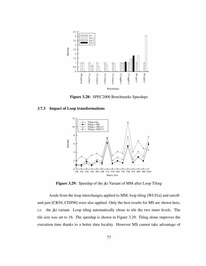
0

0.5

1

1.5

2

2.5

3

3.5

4

4.5

301.apsi.2

301.apsi.1

173.applu.2

173.applu.1

171.swim

.4

171.swim

.3

171.swim

.2

171.swim

.1

168.upwise

Spee

dup

Benchmarks

LnLn-1Ln-2Ln-3

Figure 3.28: SPEC2000 Benchmarks Speedups

3.7.3 Impact of Loop transformations

0

2

4

6

8

10

12

128 192 256 320 384 448 512 576 640 704 768 832 896 960 1024

Spee

dup

Matrix Size

Tiling onlyTiling + MSTiling + SSP L3Tiling + SSP L5

Figure 3.29: Speedup of the jki Variant of MM after Loop Tiling

Aside from the loop interchanges applied to MM, loop tiling [WL91a] and unroll-

and-jam [CK94, CDS96] were also applied. Only the best results for MS are shown here,

i.e. the jki variant. Loop tiling automatically chose to tile the two inner levels. The

tile size was set to 16. The speedup is shown in Figure 3.29. Tiling alone improves the

execution time thanks to a better data locality. However MS cannot take advantage of

77

it and the performance decreases by 38% when MS is used whereas SSP, applied to the

middle (L3 after loop tiling), benefits from the tiling. The reason for such a difference is

the cost of the prolog and epilog induced by the loop tiling. Because several iterations are

scheduled in the same group, the SSP schedule can amortize such a cost.

0

1

2

3

4

5

64 128 192 256 320 384 448 512 576 640 704 768 832 896 960 1024

Spee

dup

Matrix Size

U&J onlyU&J + MSU&J + SSP L3U&J + SSP L5

Figure 3.30: Speedup of the jki Variant of MM after Unroll-and-Jam

Unroll-and-Jam applied to the same variant of MM in Figure 3.30 has the same

impact. The transformation was applied on the already loop tiled code, which is used as

a reference for the speedup curves. The optimization alone brings a performance boost,

which is decreased by MS but amplified with SSP at both the L3 and L5 levels.

Both transformations increase the depth of the loop nest and decrease the number

of iterations of the innermost loop. Therefore the relative execution time of the prolog

and epilog at the innermost level becomes more important. However, because SSP can be

applied to other levels than the innermost, this limitation does not exist and SSP schedules

can take advantage of both transformations.

3.7.4 Cache Misses Analysis

In this section, we consider the cache misses to help explain further the previous

results. Because our loop nests come from scientific applications rich in floating-point

78

0

0.2

0.4

0.6

0.8

1

1.2

1.4

1.6

U&J jkitiled jkikjikijjkijikikjijk

Rel

ativ

e C

ache

Mis

ses

Benchmarks

MSSSP L1SSP L2SSP L3SSP L5

(a) L2 Cache Misses

0

0.2

0.4

0.6

0.8

1

1.2

1.4

1.6

U&J jkitiled jkikjikijjkijikikjijk

Rel

ativ

e C

ache

Mis

ses

Benchmarks

MSSSP L1SSP L2SSP L3SSP L5

(b) L3 Cache Misses

Figure 3.31: Cache Misses Results for the MM Variants

79

operations and because floating-point values bypass the L1 cache in the Itanium archi-

tecture, only the L2 and L3 cache misses are of interest. The L1 cache misses are only

due to instruction cache misses. The L2 and L3 cache misses results are shown for all the

variants of MM in Figures 3.31(a) and 3.31(b) respectively.

Overall, without any form of tiling, SSP has no negative impact on the number of

cache misses. Every time SSP is applied to the outermost loop, they are even lowered,

which would explain the better execution times. With loop tiling and unroll-and-jam,

it is however not the case. Indeed the grouping of iterations in SSP induces some data

requests that are different from what both optimizations had anticipated. However the

quality of the SSP schedules and the higher level of instruction-level parallelism offsets

such a drawback. Also, not every cache miss results in a pipeline stall. The study of the

relationship between tile size and group size in SSP is left for further research however.

It is very likely that such research will lead to different solutions than MS because of the

different memory access patterns of the SSP schedules.

3.8 Related Work

3.8.1 Hierarchical Scheduling

Lam [Lam88] proposed using hierarchical scheduling to software-pipeline loop

nests. The innermost loop is first software-pipelined and then considered as a single

operation when software-pipelining the second loop in the nest. As opposed to Wood’s

work [Woo79], the already software-pipelined loop is not a black box and other operations

can be scheduled in the same cycle as long as resource and dependence constraints are

honored. The main limitation is the fact that the inner loops must be software-pipelined

first. The scheduler might run out of resources very quickly or earlier decisions made

for the inner loop might prevent getting the most out of the outer loops. An example is

shown in Figure 3.32. The innermost loop is software pipelined first. Then, the software

pipelined instructions formed a virtual instruction that is used to software pipeline the

outermost loop. Operation op1 now overlaps the instruction blocks and the loop nest takes

80

3 less cycles to execute than with SWP only. For SWP, the outermost loop is not software

pipelined and therefore the op1 instruction does not overlap any other instruction.

Moon and Ebcioglu [ME97] also uses hierarchical scheduling. The kernel of the

innermost loop is a single VLIW instruction word. The operations of the prolog and

epilog are reinjected in the outer loop as normal operations. Selective scheduling is then

applied to the outer loop. The algorithm suffers from the same limitations as [Lam88].

3.8.2 Software-Pipelining with Loop Nest Optimizations

Although SWP is very powerful, it has a very severe limitation: SWP can only be

applied to single loops. When scheduling a loop nest of two or more embedded loops,

only the innermost loop can be software-pipelined. However the innermost loop is not

necessarily the most profitable loop to optimize. The other loops might exhibit better

properties like instruction-level parallelism (ILP) or data locality. To overcome this hur-

dle, several loop optimizations have been applied to improve the scheduling properties of

the innermost loop in a loop nest [Muc97].

Loop interchange and loop permutation [AK84, WL91b, WL91a] can be applied

to move one of the outer loops to the innermost level. Then SWP can be used to schedule

the new innermost loop. Unfortunately this method may not solve the problem: strong

data dependencies might prevent the outer loop to be moved in place of the innermost

loop.

Loop skewing [Wol86, WL91b, WL91a] changes the shape of the iteration space

into a more useful form. Some negative dependences can be transformed into positive

dependence. Because negative data dependencies prevent the usage of other loop trans-

formations, loop skewing is often used to enable other loop optimizations. The transfor-

mation is performed by applying a linear function to the indices of the loops.

Loop tiling[Wol92, WL91a] groups iterations in the iteration space together into

tiles. Tiles are then processed one by one during the loop nest execution. Tiling allows for

better usage of data locality. However, the loop transformation increases the depth of the

81

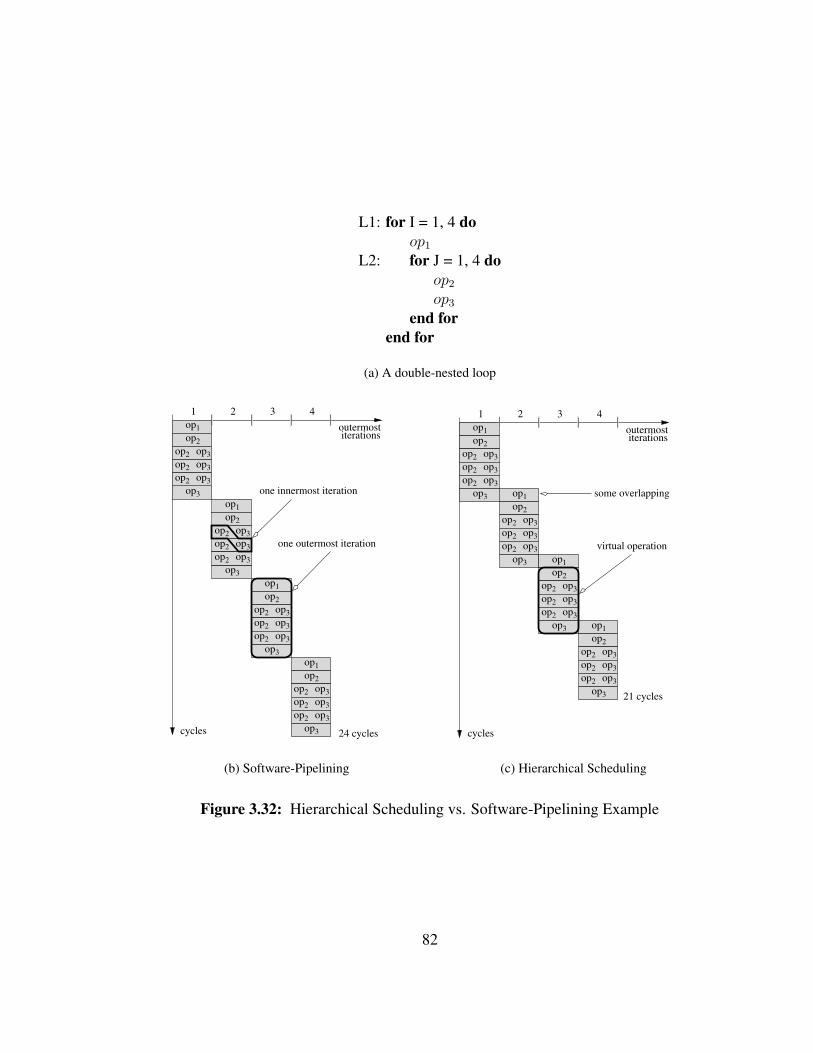
L1: for I = 1, 4 doop1

L2: for J = 1, 4 doop2

op3

end forend for

(a) A double-nested loop

cycles 24 cycles

iterations

1 2 3 4



op1op2

op2 op3

op3

op2 op3op2 op3

op1op2

op2 op3

op3

op2 op3op2 op3

op1op2

op2 op3

op3

op2 op3op2 op3

op1op2

op2 op3

op3

op2 op3op2 op3

outermost

(b) Software-Pipelining

cycles

iterations

21 cycles

1 2 3 4

virtual operation

some overlapping

op1op2

op2 op3

op3

op2 op3op2 op3

op1op2

op2 op3

op3

op2 op3op2 op3

op1op2

op2 op3

op3

op2 op3op2 op3

op1op2

op2 op3

op3

op2 op3op2 op3

outermost

(c) Hierarchical Scheduling

Figure 3.32: Hierarchical Scheduling vs. Software-Pipelining Example

82

loop nest and the overall cost of loop control overheads. Moreover, finding the optimal

tile size remains a challenge, and performance of tiled loop nests quickly decreases if the

tile size is not carefully chosen.

Loop unrolling [DH79, Sar00] duplicates the body of the innermost loop by a

given unrolling factor n and divides the total number of iterations of the innermost loop

by n. Hopefully, the instruction-level parallelism of the innermost loop is increased.

The scheduler then has more opportunities to efficiently schedule the innermost loop.

Unfortunately loop unrolling multiplies the code size of the innermost loop by a factor of

n. Also, good heuristics must be used to choose the unrolling factor.

Unroll-and-jam [CCK88, CK94, CDS96] is a generalization of loop unrolling for

outer loops in a loop nest. The chosen loop level is unrolled and the inner loops are

duplicated and fused (or jammed) together. The inner loop body is therefore duplicated

as many times as the the outer loop was unrolled. The transformation is useful when the

innermost loop shows poor instruction-level parallelism and strong data dependencies.

Instead of running innermost iterations in parallel, outermost iterations are processed.

Loop unroll-and-squash [PHA02] is a code-size optimized version of loop unroll-

and-jam. There is only one copy of the inner loop body. Some register renaming tech-

niques and register copy instructions are used to preserve the correctness of the code.

A direct consequence is a reduction in code size and a better usage of the available re-

sources. The major drawback is an increase of dependences limiting the efficiency of the

SWP scheduling algorithm used afterwards.

Software thread-integration [SD05] jams procedures together to improve the

instruction-level parallelism of the code. The method can be extended to loop nests us-

ing Deep Jam [CCJ05] to generalize unroll-and-jam which brings together independent

instructions across control structures and removed memory-based dependences.

83

3.8.3 Loop Nest Linear Scheduling

Darte et al [DSRV99, DSRV02] proposed a theoretical method to enumerate all

the tight schedules for a loop nest on a given clustered processor. A tight schedule is a

schedule that fully utilizes the resources of the processor without overloading any proces-

sor. The solution is a linear schedule: the schedule time and the processor to which each

operation is assigned is a linear function of the loop indexes.

The method is theoretical and mainly used to synthesize specialized co-processors

for application-specific hardware. Therefore all hardware constraints are either not men-

tioned (such as register allocation) or solved using ad-hoc hardware solutions (loop con-

trol overheads for instance). Also the method is limited to perfect loop nests only and a

cluster of processors can only handle one iteration each cycle.

84

Chapter 4

LOOP SELECTION

The loop selection step determines which loop level will be software pipelined by

SSP. The intent is to find the most profitable loop level, where the profitability is deter-

mined by the user. For instance, the user might be interested into minimizing the power

consumption of the processor during the execution of the loop nest, or into minimizing

the execution time of the loop nest. Although loop selection heuristics are left for future

work, the computation of two important factors are presented in this chapter, both aimed

at minimizing the execution time. The first factor is the initiation interval of the selected

loop level, the second the number of cache misses.

Another factor is the number of iterations of the selected loop level. If too low, the

cost of filling and emptying the pipeline cannot be amortized. Therefore loop levels with

a low number of iterations should be avoided. The exact number depends on the target

processor.

4.1 Initiation Interval

Given a loop level, a lower initiation interval is synonymous with shorter execution

time. Indeed, if the outermost iterations are issued more often, the schedule will terminate

earlier. It is therefore important to minimize the initiation interval.

However, to compare the execution time of the entire loop nest, the initiation inter-

val of different loop levels cannot be compared with each other. The number of iterations

of each loop level and the scheduling method used for the enclosing loops not selected

for software-pipelining need to be taken into account.

85

We present here a method to compute the minimum initiation interval (MII) of a

given loop level. The method is the method used in modulo-scheduling but applied to the

1-D DDG instead of the DDG of the innermost loop.

Two types of constraints prevent the iterations of the selected loop level from be-

ing fully parallelized. The first constraint is the dependences between operations from

different iterations. The corresponding MII is named recurrence minimum initiation in-

terval (recMII). The second constraint is the number of operations that can be executed

at the same time by the target architecture. The related MII is referred as the resource

minimum initiation interval (resMII). The method to compute resMII and recMII is

described below. MII is then equal to:

MII = max(recMII, resMII) (4.1)

4.1.1 Recurrence Minimum Initiation Interval

Given the 1-D DDG of the selected loop level, recMII can be computed directly

using the following formula:

recMII = maxcycle C

δ(C)

d(C)(4.2)

where: C is a cycle in the 1-D DDG

δ(C) is the sum of the latencies of the arcs in C

d(c) is the sum of the distances of the arcs in C

Positive dependences, which are taken care of by the sequential constraint, have

no influence on recMII . Indeed, positive dependences increase the length of the 1-D

schedule (S ∗T ), by adding extra empty stages when necessary. But the initiation interval

remains constant.

86

4.1.2 Resource Minimum Initiation Interval

In the context of pipelined function units, resMII is computed for each type of

resource such integer function units, floating-point function units,...

resMII = maxresource type R

number of operations using Rnumber of resources of type R

(4.3)

For non-pipelined function units, the reader is referred to [GAG96].

4.2 Memory Accesses

The number of memory accesses per iteration can be approximated. As a rule of

thumb, if the number of memory accesses per iteration is limited, the schedule is less

likely to create cache misses and more likely to use values in registers instead. It is

therefore interesting to evaluate such factor when deciding which loop level should be

selected.

The number of memory accesses per iteration point is approximated by consider-

ing the first single scheduling group of Sn outermost iterations. Within that group, we

consider the first Sn successive slices. The iteration space is then defined by the iteration

points of the form (i1, ..., in) where 0 ≤ i1, in ≤ Sn − 1. It corresponds to a SnXSn

square in the original iteration space. The square is representative of the references that

occur normally in the SSP schedule as most of the time is spent in the innermost loops

while Sn outermost iterations are executed in parallel. The set of iteration points can be

abstracted as a localized vector space [WL91a] α = span{(1, 0, ..., 0), (0, ..., 0, 1)}.The problem can now be applied to the memory access formulation in [WL91a].

Using the same notations and definitions, we can derive the number of memory accesses

per iteration point in the square iteration space. For an uniformly generated set in this

localized space, let RST and RSS be the self-temporal and self-spatial reuse vectors, re-

spectively. Let gT and gS be the number of group-spatial equivalent classes. Then, for

the uniformly generated set, the number of memory accesses per iteration is equal to:

gS + gT−gSl

le ∗ SdimRSS ∩ α(4.4)

87

where:

l is the cache line size

e =

0 if RST ∩ α = RSS ∩ α1 otherwise

The total number of memory accesses per iteration point is then the sum of the memory

accesses per iteration point for each uniformly generated set.

88

Chapter 5

SCHEDULER

5.1 Introduction

In this chapter, we present solutions to the SSP kernel generation problem. The

kernel is generated after the loop selection and data dependence graph simplification steps

(Figure 3.6). The input data are the 1-D DDG and the set of loop nest operations to sched-

ule. The output is the 1-D schedule. Generating kernels is not a simple task - as it involves

the overlapping of operations from several iteration levels (dimensions) of a loop nest, a

challenge not encountered in traditional software pipelining. In SSP kernels, there is one

subkernel per loop level in the loop nest, each one with its own initiation interval. Those

subkernels interact with each other and optimizing one subkernel could have a negative

impact on the others. Moreover, when the scheduler fails and the initiation interval must

be increased, which subkernel should be chosen? The challenge is to generate a kernel

that will, at the same time, minimize the execution time of the final multi-dimensional

schedule.

Three approaches are proposed and studied. First, the level-by-level approach

schedules the subkernel one by one starting from the innermost. Once a subkernel has

been scheduled, it cannot be undone. Second, the flat approach does not lock a subkernel

once fully scheduled. Operations from any loop level may be considered and undo pre-

vious decisions made in a different subkernel. A larger solution space can therefore be

explored. Finally, the hybrid approach schedules the innermost subkernel first and locks

it. The other operations are then scheduled using the flat method. It allows for a shorter

89

compilation time than the fast method while exploring a large solution space and focusing

resources on the innermost loop.

The proposed approaches and heuristics associated with them have been imple-

mented in the Open64/ORC compiler and analyzed on loop nests from the Livermore,

SPEC2000, and NAS benchmarks. Experimental results show that the hybrid approach

avoids the pitfalls of the two other approaches and produces schedules on average twice

faster than modulo-scheduling schedules. Because of its large search space, the flat ap-

proach may not reach a good solution fast enough and showed poor results.

The rest of the chapter is organized as follows. In the next section, the SSP kernel

generation problem for SSP, along with the associated issues, is explained. Section 5.3

presents the scheduling methods in detail. The last three sections are devoted toward

experimental results, related work, and conclusion, respectively.



The kernel generation step consists of computing a one-dimensional schedule for

the loop nests. Using the 1-D DDG, each operation is assigned a schedule time. That

time is the schedule of the first instance of the operation in the final schedule. Given an

operation op, its 1-D schedule time, i.e. its final schedule time of its outermost iteration

0 instance, is noted σ(op, 0).

The schedule time of the operations must obey the constraints presented in Sec-

tion 3.5 and shown in Figure 5.1 where the UnusedCycles function is defined as fol-

lows. Let p1 and p2 be the stage index of operations op1 and op2, respectively. If

σ(op1, 0) ≤ σ(op2, 0) and p1 = p2, then

UnusedCycles(op1, op2, k) = k ∗s=S−1∑

s=0

(T − Tlevel(s)) (5.4)

90


σ(op, i1 + 1) = σ(op, i1) + T (5.1)


σ(op1, i1) + δ ≤ σ(op2, i1 + k)− UnusedCycles(op1, op2, k) (5.2)





σ(op, 0) + δ ≤ Sp ∗ Tn (5.3)





Figure 5.1: 1-D Schedule Constraints in the Case of Imperfect Loop Nests and MultipleInitiation Intervals

91

If σ(op1, 0) ≤ σ(op2, 0) and p1 < p2, then

UnusedCycles(op1, op2, k) =

s=p2−1∑

s=p1+1


+k ∗s=S−1∑

s=0

(T − Tlevel(s)) (5.5)

Otherwise, if σ(op1, 0) > σ(op2, 0), the function is defined as:

UnusedCycles(op1, op2, k) =s=S−1∑

s=p1+1

(T − Tlevel(s)) +

s=p2−1∑

s=0

(T − Tlevel(s))

+Tblevel(p2) + Talevel(p1)

+k ∗s=S−1∑

s=0

(T − Tlevel(s)) (5.6)

The SSP kernel generation problem can then be formulated as follows: given a

set of loop nest operations and the associated 1-D DDG, schedule the operations so that

the scheduling constraints are honored and the initiation interval of each subkernel is

minimized. Even in the simplest case, where the loop nest is a single loop, the problem is

NP-hard [Woo79].

5.2.2 Issues

The kernel generation problem raises several challenges. First, the scheduling

constraints must be honored. The difficulty resides in the constraints that did not exist

in modulo scheduling, namely the dependence constraints, the sequential constraints and

the innermost level separation constraints. As the kernel is being generated, its final

parameters are unknown until the scheduling is complete. Therefore, it is impossible to

know the number of stages per cycle until then. However, that number is required to be

able to honor the dependence constraints and the innermost level separation constraint.

Second, unlike modulo scheduling, the kernel is composed of subkernels with

different initiation intervals which must be respected during the scheduling process. For

92

op1op2op3

op5op1

op2op3

op4op5place op4

op3 is ejectedinnermost II = 2

Figure 5.2: Strict Initiation Rate of Subkernels

instance, in Figure 5.2, the II of the innermost kernel is 2. When inserting op4, op3 must

be ejected to maintain the current II.

op1op2op3

op5 subkernelschedule

1 cycle later

truncated subkernel

op1op3

op2op5

Figure 5.3: Truncation of Subkernels

Also, the integrity of each subkernel must be guaranteed. If a subkernel is resched-

uled to a different cycle, one must make sure that that subkernel is not truncated as shown

in Figure 5.3

Finally, there is the problem of deciding which initiation interval to increment in

case the scheduler fails to find a solution with the given initiation intervals. In the single

loop case, the II of the loop was simply incremented. In the SSP case, we have the choice

between all the loops of the loop nests. A wrong decision can lead to a non-optimal

decision, as shown in the example in Figure 5.4(a), or might not even solve the problem

that lead to the scheduler failure, as shown in Figure 5.4(b).

5.3 Solution

5.3.1 Overview

The algorithm framework, shared by the three approaches, is derived from Huff’s

algorithm [AJLA95, Rau94, Huf93] and shown in Fig. 5.5. Starting with the initiation in-

tervals set to their respective minimum initiation interval value, the scheduler proceeds

as follows. The minimum legal scheduling distance (mindist) between any two de-

pendent operations is computed. Using the mindist information, the earliest and latest

93

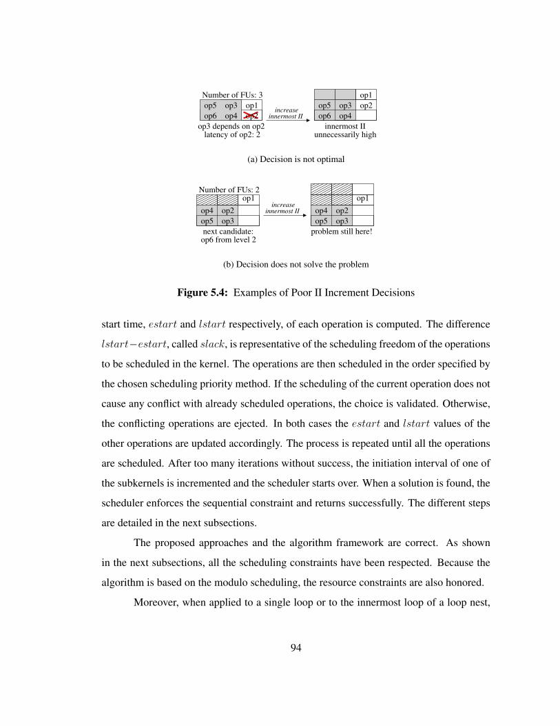
op3 depends on op2

Number of FUs: 3op3op4

op5op6

op1op2op1op3

op4op5op6 op2 innermost II

increase

innermost IIunnecessarily highlatency of op2: 2

(a) Decision is not optimal

next candidate:op6 from level 2

Number of FUs: 2

problem still here!

increaseinnermost IIop2

op3op4op5

op1op2op3

op4op5

op1

(b) Decision does not solve the problem

Figure 5.4: Examples of Poor II Increment Decisions

start time, estart and lstart respectively, of each operation is computed. The difference

lstart−estart, called slack, is representative of the scheduling freedom of the operations

to be scheduled in the kernel. The operations are then scheduled in the order specified by

the chosen scheduling priority method. If the scheduling of the current operation does not

cause any conflict with already scheduled operations, the choice is validated. Otherwise,

the conflicting operations are ejected. In both cases the estart and lstart values of the

other operations are updated accordingly. The process is repeated until all the operations

are scheduled. After too many iterations without success, the initiation interval of one of

the subkernels is incremented and the scheduler starts over. When a solution is found, the

scheduler enforces the sequential constraint and returns successfully. The different steps

are detailed in the next subsections.

The proposed approaches and the algorithm framework are correct. As shown

in the next subsections, all the scheduling constraints have been respected. Because the

algorithm is based on the modulo scheduling, the resource constraints are also honored.

Moreover, when applied to a single loop or to the innermost loop of a loop nest,

94

SSP SCHEDULER(approach, mii[], priority, ii incr method):for each loop level i do

set ii[i] to mii[i]end forattempts← 0while (attempts < max attempts) do

initialize mindist table, MRTcompute slack valuesplaced ops← 0while (placed ops < max placed ops) do

choose next operation op according to approach and priorityif no operation left then

enforce sequential constraintsreturn success

end ifschedule operation opplaced ops← placed ops+ 1eject operations violating resource constraints with opeject operations violating dependence constraints with opeject operations violating innermost level separation limitation with opupdate slack and MRT

end whilechoose level i to increase II according to ii incr methodii[i]← ii[i] + 1attempts← attempts+ 1

end whilereturn failure

Figure 5.5: Scheduling Framework

the method becomes the Huff’s modulo scheduling algorithm. Therefore, our method

subsumes modulo-scheduling as a special case.

5.3.2 Scheduling Approaches

5.3.2.1 Flat Approach

Three different scheduling approaches are proposed. Flat scheduling treats the

loop nest as if it were “flattened” as a single loop. When backtracking, conflicting op-

erations from all levels can be ejected from the schedule. The main advantage of this

approach is its flexibility. Early decisions can always be undone. Such flexibility leads

to a larger solution space, and potentially better schedules. On the down side, the search

space might become too large and the method too slow to find a schedule solution in time.

95

5.3.2.2 Level-by-Level Approach

With level-by-level scheduling, the operations are scheduled in the order of their

loop levels, starting from the innermost. Once all the operations of one level are sched-

uled, the entire schedule becomes a virtual operation from the point of view of the enclos-

ing level and the scheduler is called again for the next loop level. The virtual operation

acts as a white box both for dependences and resource usage. A direct property is that a

subkernel computed earlier cannot be undone through backtracking. The method has the

advantage of being relatively simple and fast. However, the early scheduling decisions

made in the inner loops might prevent the scheduler from reaching optimal solutions in

the outer levels. Figure 5.6 shows an example where the level-by-level scheduler is forced

to increase the initiation interval of the outer kernel to 3 in order to schedule op1, whereas

a flat scheduler can reschedule the inner operations in other scheduling cycles and produce

a final kernel with II = 2.

op2op3

op4

op2op3

op4 op1

op2op3

op4op1

op2op3

op4op1

innermost kernel(fixed)

resource conflictwith op2 and op4

latency conflictwith op2

final kernelII = 3

increase IIplace op1

(a) Level-by-Level Scheduling Solution

op1op2op3

op1op2op3

op1op2op3

op4 place op2 place op4

final kernelII = 2

resource conflicteject op2 and op4

op4

(b) Flat Scheduling Solution

Figure 5.6: Advantage of the Flat Approach over the Level-by-Level Approach

96

5.3.2.3 Hybrid Approach

The hybrid approach embeds the flat scheduling into a level-by-level framework.

The innermost level is scheduled first. Its kernel becomes a virtual operation and the flat

scheduling method is used for the other loop levels. The hybrid approach is intuitively a

good compromise between level-by-level and flat scheduling, as confirmed by the experi-

mental results. It can find better solutions than the level-by-level method without the high

compilation time.

5.3.3 Enforcement of the Scheduling Constraints

As the scheduling algorithm is based on Huff’s algorithm, the modulo property

and the resource constraints are naturally respected. The other constraints are also hon-

ored as explained in the following subsections.

5.3.3.1 Dependence Constraint

The dependence constraints are enforced through the mindist table. The min-

imum distance between operations op1 and op2, mindist(op1, op2), is the minimum

scheduling distance, σ(op2, 0) − σ(op1, 0), above which the dependence constraint be-

tween op1 and op2 is guaranteed to be respected. To compute the minimum distance

between two operations, we use the dependence constraint. If there is a dependence be-

tween two operations op1 and op2 with a latency of δ and a distance of k, then we must

have:

σ(op2, 0)− σ(op1, 0) ≥ δ − k ∗ T + UnusedCycles(op1, op2, k) (5.7)

Because the mindist value is statically computed once and for all before the oper-

ations are scheduled, we need to express the distance σ(op2, 0)−σ(op1, 0) independently

of the schedule time of op1 and op2. Since the exact value of UnusedCycles(op1, op2, k)

depends of those times, approximations must be made. A tight upper bound is presented

in Lemma 5.1.

97

Lemma 5.1[σ(op2, 0)− σ(op1, 0)

T+ (k + 1) ∗ S + 2

]∗ (T − Tn) (5.8)

is a tight upper bound of UnusedCycles(op1, op2, k).

Proof. We first prove that the value is an upper bound of UnusedCycles(op1, op2, k),

then that the bound is a tight bound. We will be using two properties:

T − Ti ≤ T − Tn ∀i ∈ [1, n] (5.9)

x− 1 < bxc ≤ x ∀x (5.10)

• If σ(op1, 0) ≤ σ(op2, 0) and p1 = p2, then

UnusedCycles(op1, op2, k)

= k ∗s=S−1∑

s=0

(T − Tlevel(s))

≤ k ∗s=S−1∑

s=0

(T − Tn), using 5.9

= (k ∗ S) ∗ (T − Tn)

• If σ(op1, 0) ≤ σ(op2, 0) and p1 < p2, then


=

s=p2−1∑

s=p1+1

(T − Tlevel(s)) + Tblevel(p2) + Talevel(p1) + k ∗s=S−1∑

s=0

(T − Tlevel(s))

≤s=p2−1∑

s=p1+1

(T − Tn) + Tblevel(p2) + Talevel(p1) + k ∗s=S−1∑

s=0


≤s=p2−1∑

s=p1+1

(T − Tn) + 2 ∗ (T − Tn) + k ∗s=S−1∑

s=0

(T − Tn), by def. of Ta/Tb

= [p2 − p1 + 1 + k ∗ S] ∗ (T − Tn)

=

[⌊σ(op2, 0)

T

⌋−⌊σ(op1, 0)

T

⌋+ k ∗ S + 1

]∗ (T − Tn), by definition of pi

≤[σ(op2, 0)− σ(op1, 0)

T+ k ∗ S + 2

]∗ (T − Tn), using 5.10

98

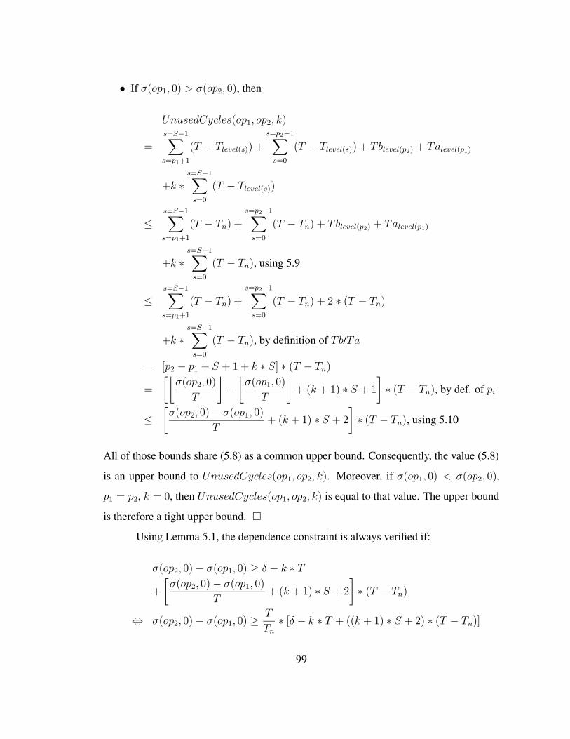
• If σ(op1, 0) > σ(op2, 0), then


=s=S−1∑

s=p1+1

(T − Tlevel(s)) +

s=p2−1∑

s=0


+k ∗s=S−1∑

s=0

(T − Tlevel(s))

≤s=S−1∑

s=p1+1

(T − Tn) +

s=p2−1∑

s=0

(T − Tn) + Tblevel(p2) + Talevel(p1)

+k ∗s=S−1∑

s=0


≤s=S−1∑

s=p1+1

(T − Tn) +

s=p2−1∑

s=0

(T − Tn) + 2 ∗ (T − Tn)

+k ∗s=S−1∑

s=0

(T − Tn), by definition of Tb/Ta

= [p2 − p1 + S + 1 + k ∗ S] ∗ (T − Tn)

=

[⌊σ(op2, 0)

T

⌋−⌊σ(op1, 0)

T

⌋+ (k + 1) ∗ S + 1

]∗ (T − Tn), by def. of pi

≤[σ(op2, 0)− σ(op1, 0)

T+ (k + 1) ∗ S + 2

]∗ (T − Tn), using 5.10

All of those bounds share (5.8) as a common upper bound. Consequently, the value (5.8)

is an upper bound to UnusedCycles(op1, op2, k). Moreover, if σ(op1, 0) < σ(op2, 0),

p1 = p2, k = 0, then UnusedCycles(op1, op2, k) is equal to that value. The upper bound

is therefore a tight upper bound. �Using Lemma 5.1, the dependence constraint is always verified if:

σ(op2, 0)− σ(op1, 0) ≥ δ − k ∗ T

+

[σ(op2, 0)− σ(op1, 0)

T+ (k + 1) ∗ S + 2

]∗ (T − Tn)

⇔ σ(op2, 0)− σ(op1, 0) ≥ T

Tn∗ [δ − k ∗ T + ((k + 1) ∗ S + 2) ∗ (T − Tn)]

99

empty

1KK2Kn

position of innerkernels may vary

length of schedulingblocks may vary

BEFOREAFTER INNERMOST

Figure 5.7: Scheduling Blocks Example

The scheduling distance between op1 and op2 is now bounded by a value in-

dependent from the schedule time of both operations. That value is used to initialize

mindist(op1, op2). By construction, it guarantees that the dependence constraint is al-

ways enforced.

5.3.3.2 Sequential Constraint

The sequential constraint is not enforced during the scheduling process, but as

a posteriori transformation once a schedule that satisfies all other constraints has been

found. The schedule is then scanned and the sequential constraint checked. If it is not

honored between two operations, empty stages are inserted in the schedule until it is

honored. The case occurs rarely enough to justify such a technique.

5.3.3.3 Innermost Level Separation Constraint

To enforce the innermost level separation limitation without any extra computation

cost, the schedule is conceptually split into three scheduling blocks: before, innermost

and after. Operations that lexically appear before ( or after, respectively) the innermost

loop are scheduled independently into the ’before’ (’after’) scheduling block as shown

in Figure 5.7. Innermost operations are scheduled into the ’innermost’ scheduling block.

Within each scheduling block, the length of the schedule may vary without breaking the

separation limitation and final length of the full schedule is only known at the very end.

The modulo resource reservation table is shared between the three blocks.

100

When an operation is scheduled or when an operation is ejected, the slack of de-

pendent operations must be recomputed. In modulo scheduling, such an update is incre-

mental and only operations that need it are updated. The SSP case is slightly different.

A dummy START and a dummy STOP operations are inserted and pre-scheduled at the

beginning and the end of each of the three scheduling blocks. If a dummy operation of

one block is ejected and rescheduled, because the distance between operations are related

with the length of each block, the slack of every operation within this block has to be

recomputed.

5.3.4 Subkernels Integrity

In the flat approach, the initiation intervals are enforced by scheduling the opera-

tions first within the current boundaries of their respective subkernel. If impossible, the

operation is scheduled at some other cycle. The subkernel boundaries are then moved cor-

respondingly. All the operations that are not scheduled within those boundaries anymore

are ejected. In the level-by-level approach, the problem never arises as the subkernels are

scheduled separately.

In the level-by-level approach, the truncation of subkernels is prevented by mark-

ing as off-limit the cycles that would lead to the truncation of a subkernel. With the flat

approach, the problem does not exist because the subkernels are never locked until the

schedule has been computed.

5.3.5 Scheduling Priority

The order in which operations are selected for scheduling influences the final

shape of the kernel. The following primary scheduling priorities based on the level of

operations are used. In innermost first order, the operations are scheduled in depth order,

starting from the innermost. In lexical order, the operations are scheduled in the order

they appear in the original source code. The lexical order follows the order of most of

the dependencies in the 1-D DDG. In block lexical order, the operations are scheduled in

101

the order of scheduling blocks: before-innermost-after. The scheduling order follows the

natural order of the execution of the loops and of most dependencies. Finally, in unsorted

order, the loop level of the operations does not influence the scheduling priority.

After the primary scheduling priorities, three secondary scheduling priorities are

used to break ties. With slack priority the operations with a smaller slack are scheduled

first. Critical operations, i.e. operations that use any critical resource (a resource used

90% of the time or more in the schedule), have their slack divided by two to increase their

priority. With smaller lstart priority the operations with a smaller latest start time are

scheduled first. The priority can be seen as a top-down scheduling approach. And with

larger estart priority the operations with a larger earliest start time are scheduled first. It

is a bottom-up scheduling approach.

5.3.6 Operation Scheduling

Once an operation has been chosen as the next candidate for scheduling, a sched-

ule cycle that satisfies the dependence constraints, the resource constraints and the inner-

most level separation constraint must be found. There are several steps to choose such a

cycle. First, one must identify the range of legal cycles where to schedule the operation.

An operation can be scheduled between its estart and lstart values. If the operation is to

be scheduled in a top-down approach, find the smallest cycle within that range. Make sure

that the operation is scheduled within the initiation interval of the loop level it belongs to,

and that it only uses available resources. If the operation is to be scheduled in a bottom-up

approach, find the latest cycle satisfying the same conditions. If the operation was sched-

uled but has been ejected since, start the search after the cycle it was scheduled to save

time. If no cycle could be found, ignore the other scheduled operations, the availability

of resources, and the initiation interval of the level of the operation. If the operation is

the virtual operation, then schedule it only where it will not be truncated. Operations that

may be in conflict with the candidate operation will be ejected and rescheduled later.

102

5.3.7 Initiation Interval Increment Methods

When the scheduler fails to find a solution with the current set of initiation inter-

vals, one loop level must be chosen and its initiation interval incremented by one. Several

approaches are proposed. With lowest slack first, the average slack of the operations of

each level is computed. The initiation interval of the loop level with the lowest average

slack value is incremented. With innermost first, used in conjunction with the innermost

first scheduling priority, the levels are considered from the innermost to the outermost.

The first level that did not manage to schedule all its operations is chosen to increase the

initiation interval. Its inner loops do not need to increase their initiation intervals because

they, at some point during the scheduling process, managed to have all their operations

scheduled. Finally, with lexical, used in conjunction with the lexical scheduling priority,

the first loop level in lexical order that did not manage to schedule all its operations is

chosen to increase the initiation interval.

The last two approaches, innermost first and lexical, are dependent on the chosen

scheduling priority scheme. They cannot be used for other scheduling priorities.

5.4 Experiments

The proposed solution was implemented in the Open64/ORC2.1 compiler. 19

loop nests of depth 2 or 3, extracted from the NAS, SPEC2000, and Livermore benchmark

suites, were software-pipelined at the outermost level and run on an Itanium2 workstation.

Each schedule was run three times on an Itanium workstation and the average time of the

three runs compared to the same loop nest scheduled using modulo-scheduling on the

innermost loop.

Results show that the hybrid approach avoids the pitfalls of the two other ap-

proaches and produces schedules on average twice faster than modulo-scheduling sched-

ules. Because of its large search space, the flat approach may not reach a good solution

fast enough and showed poor results in few cases. The level-by-level approach is more

scalable and less dependent on the choice of the scheduling priority.

103

5.4.1 Comparison of the Scheduling Approaches

For each loop level of each loop nest, the best schedules given by each method

was compared to the others. The results are shown in Figure 5.8. On average, hybrid

and level-by-level schedules are twice faster than MS schedules. In several occasions,

the flat solution is slower. Even when given as much as 10 times more attempts to find

a solution, the flat scheduler fails and had to increment the initiation intervals, resulting

in a slower final schedule. In one case (liv-5), the flat schedule was able to perform

better than the level-by-level approach. As expected, the hybrid approach combined the

advantages of the two other methods and, for all benchmarks but liv-3, produces a kernel

with best execution time. Therefore, the hybrid approach should be the method of choice

to generate SSP kernels.

1

2

3

4

5

AV

G

mm

-kji

mm

-kij

mm

-jki

mm

-jik

mm

-ikj

mm

-ijk

liv-2

3

liv-1

8.3

liv-1

8.2

liv-1

8.1

liv-7

liv-5

liv-4

liv-3

liv-2g3

blas

hydr

o

sor

Spee

dup

vs. M

odul

o Sc

hedu

ling

FlatLevel-by-LevelHybrid

Figure 5.8: Execution Time Speedup vs. Modulo Scheduling

The register pressure was also measured. On average, the register pressure in

SSP schedules is 3.5 times higher than with MS schedules, in line with results from

previous publications. The hybrid and level-by-level approaches have comparable register

pressures, whereas the pressure is lower for the flat approach as the initiation intervals are

higher. For hydro, the register pressure was too high with the level-by-level approach.

It was observed that the register pressure is directly related to the speedup results. The

104

higher the initiation intervals, the lower the register pressure and the execution time of the

schedules.

5.4.2 Comparison of the Scheduling Priorities

Figure 5.9 compares the results of the different scheduling priorities for each

scheduling approach. The minimum execution time and register pressures were recorded

and the relative difference of each heuristic to the minimum was computed for each test

case. The average is shown in the figure. The first letter U, L, I, or B stands for the

primary selection method: Unsorted, Lexical, Innermost first or Block lexical respec-

tively. The second letter S, E, or L stands for the secondary method: Slack, largest Estart

or smallest Lstart. Level-by-Level scheduling was only tested for the unsorted primary

method because all methods are equivalent when loop levels are scheduled one level after

the other.

0

0.05

0.1

0.15

0.2

0.25

B/E

B/L

B/SI/E

I/LI/S

L/E

L/LL/S

U/E

U/L

U/S

Ave

rage

Slo

wdo

wn

execution timeregister pressure

(a) Flat

0

0.05

0.1

0.15

0.2

0.25

U/E

U/L

U/S

Ave

rage

Slo

wdo

wn


(b) Level-by-Level

0

0.05

0.1

0.15

0.2

0.25

B/E

B/L

B/SI/E

I/LI/S

L/E

L/LL/S

U/E

U/L

U/S

Ave

rage

Slo

wdo

wn


(c) Hybrid

Figure 5.9: Comparison of the Scheduling Priorities

The flat scheduler appears to be highly dependent on the scheduling priority used.

There is no clear best priority. On average, each heuristic gives a solution 7.5% slower

than the best heuristic for a given loop nest while the integer register pressure is on average

18% higher. The best compromise can be found with B/S and L/S. Those high variations

are also explained by the size of the solution space. Under the loose constraints used by

the flat scheduler, there exist several correct solutions that can be attained.

105

Under tighter constraints, used by the level-by-level scheduler and indirectly by

the hybrid approach, those variations disappear. The choice of the scheduling priority

seems to have a limited influence on the quality of the computed solution.

5.4.3 Comparison of the Initiation Interval Increment Method

Figure 5.10 compares the initiation interval increment heuristics for the flat and

hybrid schedulers where appropriate. As before, the average relative difference to the

minimum for each test case under the same scheduling approach is measured. The three

heuristics, lowest Slack, Innermost first, and Lexical, are noted S, I, and L, respectively.

0

0.1

0.2

0.3

LIS

Ave

rage

Slo

wdo

wn

(a) Flat

0

0.1

0.2

0.3

LIS

Ave

rage

Slo

wdo

wn

(b) Hybrid

Figure 5.10: Comparison of the Initiation Interval Increment Methods

For the flat scheduler, the lexical order produces the fastest schedules. One may

add that the register pressure is higher though. Indeed, because the best level is chosen

when the initiation interval is incremented, a solution with a lower initiation intervals

is found. In consequence, the number of stages may increase, and with it, the register

pressure. Lower execution time comes to the expense of registers.

For the hybrid scheduler, the impact of the initiation interval increment heuristics

is limited. Indeed, the innermost level, which contains most of the operations, is treated

as a special case. Therefore, there is not much scheduling pressure left for the other levels

(2 to 3 maximum).

106

5.5 Related Work

There exist several methods to schedule operations and compute a kernel in the

case of a single loop. Those methods can be separated into two categories: optimal and

heuristic-based. Optimal modulo-scheduling techniques [AG86, EDA95, GAG94, NG93,

RGSL96] are necessary for evaluation purposes but their high computation time due to

the NP-completeness of the scheduling problem make their implementations in a pro-

duction compiler impractical. Among the heuristic-based techniques, the most relevant

methods are: Iterative Modulo-Scheduling [Huf93, Rau94], Slack Modulo-Scheduling

[Huf93], Swing Modulo-Scheduling [LGAV96], Selective Scheduling [ME97] and Inte-

grated Register-Sensitive Iterative Software-Pipelining [DRG98]. Those techniques have

already been reviewed in Section 2.1.

Modulo-scheduling techniques were extended to handle loop nests through hierar-

chical reduction [Lam88, WG96, MD01], in order to overlap the prolog and the epilog of

the inner loops of successive outer loop iterations. Although seemingly similar in idea to

the level-by-level approach proposed here, hierarchical reduction software pipelines every

loop level of the loop nest starting from the innermost, dependencies and resource usage

permitting. The dependence graph needs to be reconstructed each time before scheduling

each level, and cache effects are not considered. SSP only tries to software pipeline a

single level and to execute its inner loops sequentially, thus allocating resources first to

the loop level that requires them the most. Modulo-scheduling can also been combined

with prior loop transformations [CDS96, WMC98, PHA02].

5.6 Conclusion

In this chapter, several kernel generation methods were presented. The computed

schedule must respect the scheduling constraints that have been presented in Section 3.5,

including the SSP dependence constraint, the sequential constraint, and the innermost

level separation constraint. Several issues were encountered and solutions found. Each

subkernel has its own initiation interval which must be respected. Also, a subkernel is not

107

allowed to be truncated and therefore, not every cycle is a legal scheduling cycle. Finally,

in case the scheduler cannot compute a solution in a reasonable amount of time, a decision

must be made to decide which initiation interval should be incremented.

Three scheduling approaches were proposed and studied. The level-by-level ap-

proach schedules the loops individually starting from the innermost. Once the subkernel

of a loop has been computed, it cannot be undone. The subkernel of the enclosed loop

becomes a virtual operation for the current loop level. The flat approach does not lock a

subkernel once fully scheduled. Operations from any loop level may be considered and

undo previous decisions made in a different subkernel. A larger solution space can there-

fore be explored. Finally, the hybrid approach uses the level-by-level approach for the

innermost loop and schedules the other levels using the flat approach. Several scheduling

priorities and initiation interval increment methods were also proposed. The methods are

provably correct and handle all the issues aforementioned.

The proposed approaches and heuristics were implemented in the Open64 and

analyzed on loop nests from the Livermore, SPEC2000, and NAS benchmarks. schedul-

ing constraints. Experiments demonstrated that, although the level-by-level and hybrid

approaches show comparable schedules in terms of execution and register pressure, the

hybrid method is to be preferred because it outperforms the level-by-level approach in

some cases. The flat method was victim of its own large search space and could not find

good solutions in a reasonable amount of time and had to settle for kernels with larger

initiation intervals. The choice of the heuristics have little influence on the final schedules

for the hybrid and level-by-level approach.

108

Chapter 6

REGISTER PRESSURE EVALUATION

In this chapter we present a fast method to compute the register pressure of a

SSP kernel. Only loop variants are considered, although the register pressure from loop

invariants can easily be added. The first section motivates our work, explains the issues

that we are facing and introduces some necessary notations. The second section describes

our solution to compute the register pressure of a kernel, also called MaxLive. The last

section shows our experimental results.


6.1.1 Motivation

Several motivations lead to this work. First, as it will be seen in the next chapter,

register allocation is a time-consuming process and register allocation cannot always be

found. As the loop nest gets deeper, the register pressure might increase to a point where

the register file cannot accommodate the register needs of the schedule, even with an

optimal register allocator that always returns a solution which minimizes register usage.

In those cases, calling the already time-consuming register allocator would be a waste of

time. It is therefore important to be able to measure the register pressure of a schedule

without the help of the register allocator, and to be able to do so in a short amount of time.

If the register pressure is deemed too high for the target architecture, the SSP framework

can decide, for instance, to either increase the initiation interval and recompute a new

kernel with a lower register pressure, or to choose a different loop level to schedule as


109

n−D DDG

loop nest

loop nest

loop level

(1−D schedule)

kernel

assembly code

(final schedule)

register−allocated kernel

1−D DDG register pressure oktoo highor

SelectionLoop

SimplificationDDG

GenerationKernel

GenerationCode

AllocationRegister

n−D space1−D space

Register PressureEvaluation

Figure 6.1: SSP Framework

When developing and testing the register allocator, a second use for a fast register

pressure evaluation technique arose: to be able to evaluate the quality of the register

allocator. The register pressure provides us with a lower bound for the register allocator

to compare itself to. The closer the number of allocated registers are to that lower bound,

the better the register allocator is.

Similarly, the method can be used to evaluate the impact of any scheduling method

on the register pressure in the kernel. The register pressure is independent of the register

allocation solution and therefore allows schedulers to be compared fairly.

Finally, such a measure could orient the design of future computer architectures. If

the SSP technique was to be taken into account during the development of a new processor

family, the register pressure of benchmark loop nests would help the designers to decide

of the size of the integer and floating-point register files.

It is always possible to compute the final schedule and use traditional backwards

liveness analysis to compute the register pressure. However such a method is not efficient

in both time and space (as confirmed by our experimental results). A faster method, based

solely on the 1-D kernel, would be preferred.

110

6.1.2 Notations

The time period during which the instance of scalar variable (or loop variant) is

live is called the scalar lifetime of the instance of the variable. The first and last cycles

of the scalar lifetimes are called the start cycle and end of the scalar lifetime. If a scalar

variable is defined in outermost iteration i and killed in outermost iteration j, we call the

number of outermost iterations spanned by the corresponding scalar lifetime the omega

value of the lifetime. It is defined as j− i+ 1. It also corresponds to the number of neces-

sary live-in values for that particular variant. The number of scalar lifetimes in any given

cycle of the final schedule is called the FatCover of that cycle. The register pressure of

the schedule is the maximum FatCover over every cycle and is called MaxLive.

In order for the operations to be interruptible and restartable on a VLIW machine,

a scalar lifetime starts at the beginning of its start cycle and ends at the end of its end

cycle. Therefore, if a scalar lifetime is ended by operation op1 in the same cycle as

another scalar lifetime is started by operation op2, the two lifetimes are allowed to share

the same register only if op1=op2. Those conventions match the conventions used for MS

[RLTS92].

start

end

omega=0

omega=1

a

b

c

a

b

c

FatCover11

2

2100

2

iteration i iteration i+1

Figure 6.2: Scalar Lifetimes Notations Example

Those notations are shown on a example in Figure 6.2 where a sample of an SSP

schedule is shown. A scalar lifetime is represented by a plain line, its start by a circle,

and its end by a cross. If the same operation ends a scalar lifetime and starts another, the

cross and circle will be superimposed.

111

The scalar lifetimes can be sorted in three distinct categories: global, local, and

cross-iteration. A global lifetime exists throughout the entire schedule and corresponds

to a constant variable. It is easily accounted for and can be omitted for our purpose. The

remaining scalar lifetimes are local if their omega value is zero, and cross-iteration if not.

The distinction will be essential to our solution.

As explained in the previous section, the index of a stage within an outermost

iteration may have an influence on the number of scalar lifetimes within that stage. For

the purpose of our algorithm, the first encounter of a stage within one outermost iteration

will be referred as first, while the last will be referred as last. By construction of the

final schedule, the first and last instances of a stage can only be encountered in the

Outermost Loop Pattern. Each of the Sn instances of the Outermost Loop Pattern, defined

in Chapter 8 shows a different combinations of first and last stages.


Our problem can be formulated as follows: Given an SSP 1-D schedule, evaluate

the register pressure of the final schedule. We assume that any spilling technique, if any,

has already been applied. We are only concerned with local and cross-iteration lifetimes.

For architectures with rotating registers, the register pressure corresponds to the

rotating register pressure. Static registers are only used for global lifetimes. For archi-

tectures without rotating registers, the register pressure corresponds to the static register

pressure.

It is the first time a method to compute the register pressure of an SSP schedule

is proposed. With single loops, where MS is used, the traditional technique is to count

the number of lifetimes in the kernel, also named MaxLive [RLTS92]. Our method

can be seen as its natural extension to handle the more complex issues specific to the

multidimensional case, presented in the next section. MaxLive was the chosen method

to evaluate the efficiency of register allocators in [EDA94, LAV98]. Other work [NG93]

considered the theoretical register pressure during the scheduling phase by counting the

112

number of buffers required to store results of each operation. However the number of

buffers did not take into account that some buffers could be reused. The register pressure

was also studied for non software-pipelined schedules, such as the concept of FatCover

in [HGAM92]. Llosa et al. [LAV98] used MaxLive to measure the register pressure of

floating-point benchmarks. Their results also show that a FP register file of 64 registers

would accommodate most of the register pressure and limit accesses to memory in the

case of MS scheduled loops. The results were later confirmed in [ZLAV00].

6.1.4 Issues

The problem of evaluating the register pressure of the schedule by considering the

kernel only is straightforward in the single loop case [RLTS92]. However, in the multi-

dimensional case, new issues arise.

c

dc

c

c

d

d

d

abcd

abcd

abcd

stretched scalar lifetime

of stalled outermost iterationirregular initiation rate because

T=2T=3

irregular initiation rate becauseof variable initiation interval

Figure 6.3: Irregular Pattern of the Scalar Lifetimes

First, unlike with MS, the scalar lifetimes do not exhibit a regular pattern. When

an outermost iteration is stalled, the start of the scalar lifetimes in that iteration is also

delayed. Moreover, an already started lifetime will be stretched while holding a value

until the execution of the stalled outermost iteration resumes. The problem becomes

even more complex when the initiation interval is not constant. Examples are shown in

113

Figure 6.3 where a sample of an SSP schedule is shown with the innermost stages grayed

out.

d

d

c

e

(a) Always Used, Except for the Last Instance

d

d

c

e

(b) Never Used, Except for the Last Instance

Figure 6.4: Scalar Lifetimes Variance Within Different Instances of the Same Stage

Second, given a stage and cycle within that stage, the number of scalar lifetimes

is different depending on the instance of the stage in the final schedule. For instance, in

Figure 6.4(a), a scalar lifetime starts in stage d and ends 3 cycles later in stage c. However

if it is the last instance of stage d, then the scalar lifetime is useless (but a register is still

needed for the operation in stage d. Symmetrically, in Figure 6.4(b), a scalar lifetime

always ends in the same cycle as it starts because no operation uses the value. But the

last instance of the scalar lifetime is used by stage e from an upper level. Therefore two

instances of the same scalar lifetime may have different lengths.

Finally, the method must be obviously fast enough so that schedules with a register

pressure higher than the number of available physical registers can be quickly detected in

the compilation process..

6.2 Solution

6.2.1 Overview

To quickly compute the register pressure of the final schedule using only the ker-

nel, some insight on the lifetimes in the final schedule is needed. An example is shown

in Figure 6.5. The stable phase of the final schedule, where the maximum is most likely

114

to be encountered is an alternation between Sn instances of the Outermost Loop Pattern

(OLP) and the Inner Loop Execution Segment (ILES), represented in the figure 1. The

first instance of a stage is represented by a light gray box, whereas the last instance is

represented by a dark gray box. The other instances are left white.

abd c

abd ce

e

c

c

d

d

c

c

d

db

b

1 2 3

4 5 76

7654

: stretched cross−iteration

: stretched local lifetimes: local lifetimes: stretched local lifetimesfirst

last

lifetimes

123

: local lifetimes: local lifetimes

: cross−iteration lifetimes

last

first

Legend

: instance of the stageslastfirst: instance of the stages

OLP: ILES:

Within one outermost iteration:

Figure 6.5: Scalar Lifetimes in the Final Schedule Example

During the execution of an OLP instance, the scalar lifetimes can either be local

in a first stage, local in a last stage, or cross-iteration. In the ILES segment, they can be

1 For more details about those patterns, the reader is referred to Section 3.4 or Chapter 8

115

either local or stretched lifetimes from the latest OLP instance (local first, local last, or

cross-iteration). In our solution, each type of scalar lifetimes is accounted for individually.

The FatCover at a given cycle of the final schedule can then be expressed as the sum of

the lifetimes from each type at that cycle. The final register pressure is then defined as the

maximum over all the cycles of the schedule.

The prolog and epilog phases of the final schedule are ignored. Indeed, during

those two phases, a smaller number of outermost iterations are executed in parallel, and

it is therefore highly unlikely that the register pressure may reach its peak at that moment

(although it is possible if the number of live-in values is high enough).

The following sections explain how to count each type of scalar lifetime for each

situation.

6.2.2 Cross-Iteration Lifetimes

Because the outermost loop level is the only level actually software pipelined,

only variants defined in the outermost level can have a cross-iteration lifetime. The first

step consists of identifying the cross-iteration variants. They are defined in the stages

appearing in the outermost loop only and show at least one use with an omega value

greater than 0. Then, for each variant, the stage and modulo-cycle of the definition and of

the last use are computed and noted Sdef , cdef , Skill, and ckill, respectively. The definition

of each variant is unique and therefore easily found. Because cross-iteration lifetimes

span several outermost iterations, the last use of a such lifetimes must be searched among

each of the spanned iterations. The stage index of the last use is computed by adding the

omega value of the use to its stage index.

Afterward, the number of cross-iteration variants lifetimes at modulo-cycle c in

116

COMPUTE CROSS ITERATION LT():civs← ∅ // cross-iteration variants setovs← set of the variants defined in the outermost loop

// Identify the cross-iteration variantsfor each operation op in the schedule

for each source operand src of opif omega(op, src) > 0 and src ∈ ovs thencivs← civs ∪ {src}initialize Sdef , cdef , Skill, ckill for src to −1

// Collect the parameters for each cross-iteration variantfor each stage s from l1 to f1, backwards

for each cycle c from T − 1 to 0, backwardsfor each operation op in s at cycle c

for each source operand src of op in civsif Skill(src) = s+ omega(op, src) thenSkill(src) unchangedckill(src)← max(ckill(src), c)

else if Skill(src) < s+ omega(op, src) thenSkill(src)← s+ omega(op, src)ckill(src)← c

for each result operand res of op in civscdef (res)← cSdef (res)← s

Figure 6.6: Cross-Iteration Lifetimes Algorithm

117

the OLP is then given by LTcross(c):

LTcross(c) =∑

v∈civs((Skill(v)− Sdef (v) + 1) + δdef (c, v) + δkill(c, v)) (6.1)

where

δdef (c, v) = −1 if c < cdef (v), 0 otherwise

δkill(c, v) = −1 if c > ckill(v), 0 otherwise

Skill(v) − Sdef (v) + 1 represents the length in stages of the lifetime of v. The two other

δ terms are adjustment factors to take into account the exact modulo-cycle the variant is

defined or killed in the stage. Figure 6.7 shows an example of a cross-iteration lifetime.

The lifetime starts at Sdef = 1, corresponding to stage b, and cdef = 2, and stops omega =

3 iterations later in stage Skill = 0 + omega at modulo-cycle ckill = 0. Then the number

of cross-iteration lifetimes for that variant is equal to 2, 1, and 2 at modulo-cycle 0, 1, and

2 respectively.

LTcross212

b

c

d

a

a

a

b

bc

a

omega=3

c = 0kill

S = 0kill

c = 2def

S = 1def

Figure 6.7: Cross-Iteration Lifetimes Computation Example

The number of live-out cross-iteration lifetimes corresponds to the number of life-

times at the entrance of cycle after T − 1 and is represented by LTcross(T ).

6.2.3 Local Lifetimes

The computation of the local lifetimes is done by using traditional backwards data-

flow liveness analysis on the control-flow graph of the loop nest where each loop level is

118

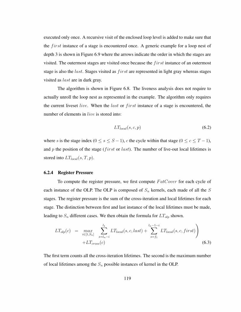
executed only once. A recursive visit of the enclosed loop level is added to make sure that

the first instance of a stage is encountered once. A generic example for a loop nest of

depth 3 is shown in Figure 6.9 where the arrows indicate the order in which the stages are

visited. The outermost stages are visited once because the first instance of an outermost

stage is also the last. Stages visited as first are represented in light gray whereas stages

visited as last are in dark gray.

The algorithm is shown in Figure 6.8. The liveness analysis does not require to

actually unroll the loop nest as represented in the example. The algorithm only requires

the current liveset live. When the last or first instance of a stage is encountered, the

number of elements in live is stored into:

LTlocal(s, c, p) (6.2)

where s is the stage index (0 ≤ s ≤ S− 1), c the cycle within that stage (0 ≤ c ≤ T − 1),

and p the position of the stage (first or last). The number of live-out local lifetimes is

stored into LTlocal(s, T, p).

6.2.4 Register Pressure

To compute the register pressure, we first compute FatCover for each cycle of

each instance of the OLP. The OLP is composed of Sn kernels, each made of all the S

stages. The register pressure is the sum of the cross-iteration and local lifetimes for each

stage. The distinction between first and last instance of the local lifetimes must be made,

leading to Sn different cases. We then obtain the formula for LTolp shown.

LTolp(c) = maxi∈[1,Sn]

(l1∑

s=ln−iLTlocal(s, c, last) +

ln−1−i∑

s=f1

LTlocal(s, c, first)

)

+LTcross(c) (6.3)

The first term counts all the cross-iteration lifetimes. The second is the maximum number

of local lifetimes among the Sn possible instances of kernel in the OLP.

119

COMPUTE LOCAL LT():// Start recursive analysis from the outermost level∀(s, c, p) ∈ [f1, l1]X[0, T ]X{first, last}LTlocal(s, c, p)← −1, Visit Level(1, ∅)

// Initialize first with last value if first uninitializedfor each stage s from f1 to l1

for each cycle c from 0 to Tif LTlocal(s, c, first) = −1 thenLTlocal(s, c, first)← LTlocal(s, c, last)

VISIT LEVEL(level level, live set live):// Count the local lifetimes for loop level ’level’for each stage s from llevel to flevel, backwards

for each cycle c from T to 0, backwardslive← live ∪DEF (s, c) ∪ USE(s, c)if LTlocal(s, c, last) = −1 thenLTlocal(s, c, last)← |live|

elseold← LTlocal(s, c, first)LTlocal(s, c, first)← max(old, |live|)

live← (live−DEF (s, c)) ∪ USE(s, c)// Recursive call for the inner levelsif level < n and s = flevel+1 then

Visit Level(level + 1, live)

Figure 6.8: Local Lifetimes Algorithm

120

l

l +1

l +1

l

l

f

f −1

f

f −1

f1

1

i

i

i

i

n

n

n

n

level 1 level 2 level 3

first

last

Figure 6.9: Local Lifetimes Computation Example

The method to compute the FatCover for any cycle in the ILES is similar. We

add the local lifetimes of the Sn stages of the current cycle to the stretched lifetimes from

the latest OLP instance (live-out values). We obtain:

LTiles(c) = LTcross(T ) +

l1∑

s=ln

LTlocal(s, T, last) +

fn−2∑

s=f1

LRlocal(s, T, first)

+ maxl∈[2,n]

(max

i0∈[0,Sl−1]

(Sn−1∑

i=0

LTlocal(fl + (i0 + i)%Sl, c, first)

))(6.4)

The first three terms correspond to the three types of stretched lifetimes: cross-iteration,

last local and first local in that order. Their number is fixed for the entire execution of

the ILES and equal to the number of lifetimes live at the exit of the OLP. The fourth term

of the formula corresponds to the local lifetimes of the ILES.

MaxLive is then the maximum between the maximum register pressure of the

121

OLP and the maximum register pressure of the ILES patterns:

MaxLive = max

(max

∀c∈[0,T−1](LTolp(c)) , max

∀c∈[0,T−1](LTiles(c))

)(6.5)

6.2.5 Time Complexity

Both routines Compute Cross Iteration LT and Compute Local LT run in

O(S ∗ II). Assuming that the loop variant sets are implemented using bit vectors,

Visit Level runs in O(II) per stage. The routine is called once for each loop level l

and visits Sl stages per call for a total of∑n

i=1 Si. Because S > Si,∀i ∈ [1, n], the fast

method algorithms run in O(n ∗ S ∗ II).

The computation time of the formulas is bounded by the two maximum operators

enclosing a sum in LTiles(c). Because Si ≤ S,∀i, the computation time of the formula

is bounded by O(S2 ∗ II ∗ n). Therefore, the overall complexity of the fast method is

bounded by: O(S2 ∗ II ∗ n).


The algorithms were implemented in the ORC 2.1 compiler and tested on an

1.4GHz Itanium2 machine with 1GB RAM running Linux. The benchmarks are SSP-

amenable loop nests extracted from the Livermore Loops, the NPB 2.2 benchmarks and

the SPEC2000 FP benchmark suite. A total of 127 loop nests were considered. When all

the different depths are tested, 328 different test cases were available. There were 127,

102, 60, 30, and 9 loop nests of depth 1, 2, 3, 4, and 5, respectively.

The straightforward method consisting of unrolling the final schedule and apply-

ing liveness analysis was also implemented for comparison. It is referred as the compre-

hensive method. Our method in contrast is referred as the fast method.

The main results are summarized here and explained in details in the next sub-

sections. (1) The fast method is 1 to 2 orders of magnitude faster than the compre-

hensive method, and 3 to 4 orders of magnitude faster than the register allocator. (2)

122

Despite the approximations made by the fast method, its computed MaxLive is identi-

cal to MaxLive computed by the comprehensive method. No rule of thumb could be

deduced to predict MaxLive by only considering the 1-D schedule parameters such as

kernel length, number of loop variants, and others. Rotating Register pressure increases

quickly for integer values as the loop nest gets deeper and about half of the loop nests

of depth 4 or 5 show a MaxLive higher than the size of the INT register file. (3) The

floating-point rotating register pressure remains about constant as the depth of the loop

nests increases, and never exceeds 47 registers. Consequently, the floating-point rotating

register file could be reduced from 96 to 64 registers. The extra 32 registers could be

added to the integer register file instead.

6.3.1 Register Pressure Computation Time

1e-04

0.001

0.01

0.1

1

10

Tim

e (s

ec,lo

g sc

ale)

Benchmarks

depth 1

depth 2

depth 3

ComprehensiveFast

Figure 6.10: Register Pressure Computation Time

The measurements of the execution time of the comprehensive and fast methods

are presented in Figure 6.10 where the loop nests have been sorted first by increasing

depth, delimited by tics on the horizontal axis, and then by increasing kernel length. Note

the logarithmic scale for the vertical axis. The comprehensive and fast methods take

up to 3.18 and 0.04 seconds respectively, with an average of 0.16 and 0.005 seconds.

123

The running time of each method is directly related to the kernel length. The shape of

the graph confirms the quadratic running time of the fast method and the influence of

the depth of the loop nest. The fast method is 22.9 times faster than the comprehensive

method, with a maximum of 217.8. As the loop nest gets deeper, the speedup becomes

exponentially more significant.

1

10

100

1000

10000

100000Sp

eedu

p (l

og s

cale

)

Benchmarks

Figure 6.11: Speedup vs. the Register Allocator

In order to use the register pressure evaluation in the SSP framework, its execu-

tion time must be noticeably lower than the execution time of the register allocator. The

execution time of the fast method and the register allocator presented in the next chapter

are compared in Figure 6.11. On average, the fast method is 3 orders of magnitude faster

than the register allocator with a maximum of 20000. As the loop nest gets deeper, i.e. as

the MaxLive increases and the need for a quick method to evaluate the register pressure

a priori becomes stronger, the speedup increases, making the fast method a valid tool to

detect infeasible schedules before actually running the register allocator.

Although the fast method does not take into account the live-in and live-out life-

times, the computed MaxLive was identical for the two other methods in all the bench-

marks tested. It confirms our assumption that MaxLive is less likely to appear in the

prolog and epilog.

124


The computed MaxLive is actually an optimistic lower bound on the actual reg-

ister pressure. It does not take into account that a value held in one register at cycle c

must remain in the same register at cycle c+1 or that the use of rotating registers reserves

a group of consecutive registers at each cycle, even if some of them are not currently

used. The actual register allocation solution computed by an optimal register allocator

may allocate more registers than MaxLive. However, with the addition of register copy

instructions, MaxLive registers can always be reached.

0

32

64

96

128

160

192

224

Max

Liv

e

Benchmarks

depth 1

depth 2

depth 3

IntegerFloating-Point

Figure 6.12: Register Pressure

The computed MaxLive is shown in Figure 6.12 for INT and FP loop variants.

The benchmarks have been sorted by increasing depth, indicated by small tics on the

horizontal axis, and by increasing MaxLive. The average MaxLive for INT and FP

are 47.2 and 15.0 respectively with a maximum of 213 and 47. If we only consider

rotating registers, the 96 hard limit on the number of available FP registers in the Itanium

architecture is never reached. However the 96 limit for INT registers is reached more often

as the depth of the loop nests increases, up to 56% for the loop nests software pipelined

at level 4 as shown in Figure 6.13.

INT MaxLive increases faster than FP MaxLive. INT MaxLive indeed in-

creases as the nest gets deeper because more inner iterations are running in parallel. It is

particularly true for INT values that are used as array indexes. If an array index is defined

125

0

0.2

0.4

0.6

0.8

1

1 2 3 4 5

Am

enab

ility

Rat

io

Depth

Figure 6.13: Ration of Loops Amenable to SSP

in the outermost loop, then there is one instance of the index for each concurrent outer-

most iteration in the final schedule. For FP values however, this is not the case. They are

typically defined in the innermost loop only and have very short lifetimes.

We also tried to approximateMaxLive by looking at the 1-D schedule parameters.

However no rule of thumb could be derived by looking at one parameter such as S, Sn, the

length of the kernel or the number of loop variants. The MaxLive was also compared to

the actual number of registers allocated by the register allocator. Unlike in MS where the

number of registers allocated rarely exceeds MaxLive+1 [RLTS92], the difference with

SSP varies between 0% and 77%. Such results are explained by the higher complexity of

SSP schedules compared to MS and because MaxLive is not a tight lower bound.

6.3.3 Register File Size

Figure 6.14 shows the total register pressure, defined as the sum of MaxLive for

INT and FP registers, on the left axis. The ratio between FPMaxLive and INTMaxLive

is shown on the right axis. The benchmarks are sorted by increasing ratio. The total

register pressure rarely exceeds 192 registers, the size of the rotating register file in the

Itanium architecture. Although FP MaxLive can be twice higher than INT MaxLive,

the FP/INT ratio remains lower than 0.5 when the total register pressure is greater than

96, the actual size of the INT register file on the Itanium architecture.

126

32

64

96

128

160

192

224

256

0

0.5

1

1.5

2

2.5

Tot

al R

egis

ter P

ress

ure

(FP+

INT

)

FP/I

NT

Rat

io

Benchmarks

Total Register PressureFP/INT Ratio

Figure 6.14: Total Register Pressure and FP/INT Ratio

Figure 6.15 shows FP MaxLive as the same loop nest is scheduled at deeper

levels. Segments on top of bars indicate an increase in FP register pressure when the loop

nest is software-pipelined at a lower level. FP MaxLive does not or barely increases as a

same loop nest is scheduled at a lower level. The maximum FP MaxLive never exceeds

47 registers. The main reason is that FP variants have very short lifetimes that mostly

appear at the innermost level of the loop nests. Scheduling a loop nest at different levels

has little influence on the number of innermost iterations running in parallel (Sn), and

therefore the number of FP scalar lifetimes appearing in the same cycle.

Several conclusions, that may be useful for future designs of architectures with

the same number of functional units and superscalar degree than the Itanium architecture,

can be drawn from these remarks. First, the INT register file may benefit from a smaller

FP register file with a ratio of 2 for 1. The FP register size can either be decreased to

save important chip real estate, or the INT register file increased to allow more SSP loops

to be register allocated. Second, for the set of benchmarks used in our experiments, the

optimal size for the FP register file would be 64. It would not prevent any other loop nests

from being register allocated while giving extra registers to the INT register file. If a size

of 64 and a INT/FP ratio of 2 are chosen, the feasibility ratio for loop nests of depth 4

127

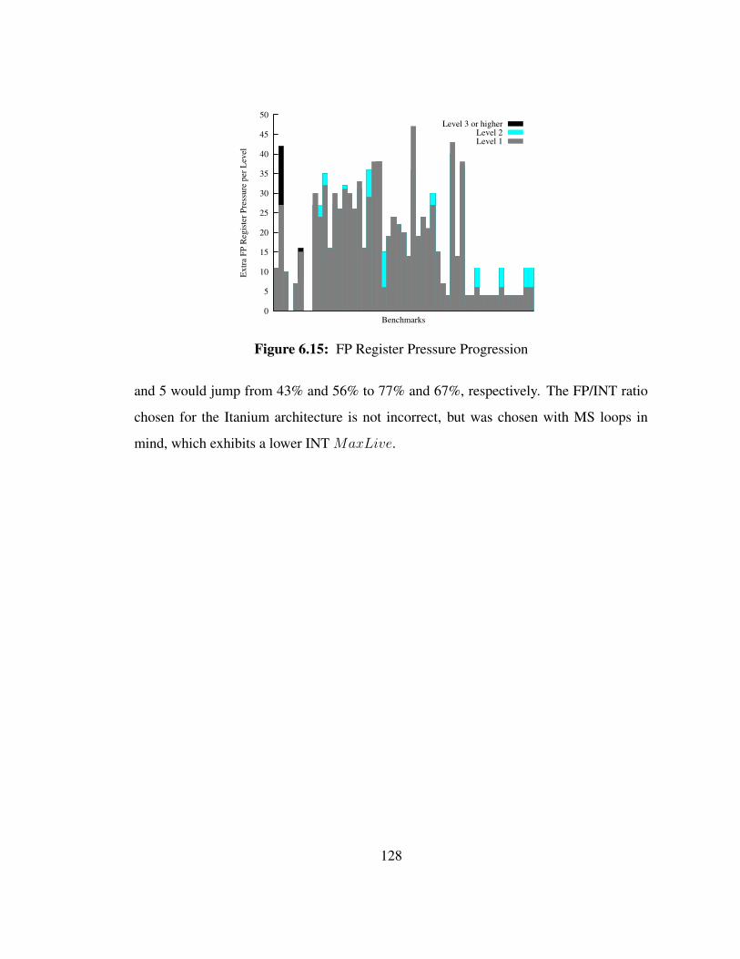
0

5

10

15

20

25

30

35

40

45

50

Ext

ra F

P R

egis

ter P

ress

ure

per L

evel

Benchmarks

Level 3 or higherLevel 2Level 1

Figure 6.15: FP Register Pressure Progression

and 5 would jump from 43% and 56% to 77% and 67%, respectively. The FP/INT ratio

chosen for the Itanium architecture is not incorrect, but was chosen with MS loops in

mind, which exhibits a lower INT MaxLive.

128

Chapter 7

REGISTER ALLOCATION

7.1 Introduction

At this point in the SSP compilation process, the kernel has already been computed

by the scheduler and the register pressure has been deemed low enough to justify trying

to allocate register to the loop variants of the kernel. This chapter presents an efficient

register allocation method for the SSP framework. It takes as input an SSP kernel and

returns a register-allocated kernel.

In this chapter we make the difference between register assignment and register

allocation. The latter describes the overall process of deciding how many registers are to

be allocated and to which loop variants. It makes sure that no interference exists between

the lifetimes of the schedule once the process is finished. On the other hand register

assignment is the act of actually assigning a specific register to a specific loop variant.

The next section describes a register allocation method used in single loops that

have been scheduled with MS. It will give the reader a quick overview of the task ahead.

Section 7.3 then presents in more details the problem of allocating registers in SSP. The

section hereafter will present our solution to the problem and its algorithms. Finally

experimental results will be shown in Section 7.5 before concluding in Section 7.7.

7.2 MS Register Allocation

In this section, we quickly review how register allocation is typically performed

with singles loops that have been scheduled using MS [RLTS92]. It will allow us to

129

introduce some concepts that will be reused later on to present the register allocation for

SSP. Unless noted otherwise, we assume for this section a single loop of N iterations and

an initiation interval of T. We assume the presence of hardware support in the form of

rotating registers.

7.2.1 Scalar and Vector Lifetimes

A scalar lifetime is the lifetime of a loop variant for a given iteration of the loop.

The variant has one operation to produce a value and one or more operations to consume

the value. It starts when the producer is issued and ends when all of the consumers have

finished. All the scalar lifetimes of the loop variant over all the iterations of the loop

compose the vector lifetime of the loop variant.

The vector lifetimes can be represented on a space-time diagram, where time is

on the horizontal axis and the registers on the vertical axis. An example with two vector

lifetimes is shown in Figure 7.1(c). A vector lifetime is composed of a wand (the diagonal

band), a leading blade in case of live-in values, and a trailing blade in case of live-out

values. The wand is made of the scalar lifetimes from iteration 0 to iteration N-1 whereas

the leading and trailing blades corresponds to iterations -1 and under, and iterations N and

above, respectively. In our example, the second vector lifetime is made of only a wand.

The first vector lifetime, because it has both a live-out value and a live-in value, has a

trailing blade and a leading blade.

A vector lifetime can be represented by a 4-tuple (start, end, omega, alpha). The

start and end values refer to the start and end cycles of the scalar lifetime produced by

the first iteration of the loop (iteration 0). The start time of the scalar lifetime of loop

iteration i is then equal to start + i ∗ T and its end time to end + i ∗ T . Omega is the

number of live-in values for the loop variant. It is also the maximum live-in distance of

all the instances of the loop variant. Alpha represents the number of live-out values for

the loop variant. For example, our two vector lifetimes are represented as (1, 3, 1, 1) and

(0, 6, 0, 0), respectively.

130

for I = 1, N doop1: y = x[1]op2: x = ...op3: ... = y

end for

(a) Source Code

op3

op1op2

op1op2

op1op2

op3

op3

(N−2 times)Kernels

Prolog

Epilog

T=2

of loop variant yscalar lifetime

(b) MS Schedule

regi

ster

s

0 2*T 3*T 4*T 5*T 6*T 7*T 8*T 9*T

time

1*T

y

x leading blade

wand

trailing blade

scalar lifetimeof iteration 0

(c) Space-Time Diagram

Figure 7.1: Vector Lifetime Examples

7.2.2 Space-Time Cylinder

A physical register Rr is said to be allocated to a vector lifetime v if it is allocated

to the first scalar lifetime of v. The ith scalar lifetime is then allocated to the physical

register number Rr−i+1.

Due to the cyclic nature of the rotating register file, the register index wraps around

to the highest register index when it becomes -1. Thus, the space-time diagram can be

seen as a cylinder where the axis represents time and the vector lifetimes are mapped onto

the surface of the cylinder. The circumference of the cylinder is then the total number of

rotating registers required by the loop.

131

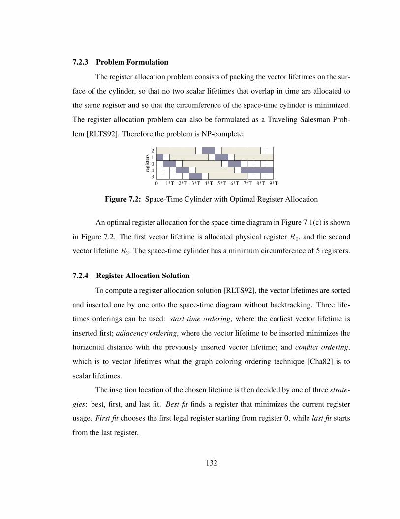
7.2.3 Problem Formulation

The register allocation problem consists of packing the vector lifetimes on the sur-

face of the cylinder, so that no two scalar lifetimes that overlap in time are allocated to

the same register and so that the circumference of the space-time cylinder is minimized.

The register allocation problem can also be formulated as a Traveling Salesman Prob-

lem [RLTS92]. Therefore the problem is NP-complete.

0 2*T 3*T 4*T 5*T 6*T 7*T 8*T 9*T1*T

043

21

regi

ster

s

Figure 7.2: Space-Time Cylinder with Optimal Register Allocation

An optimal register allocation for the space-time diagram in Figure 7.1(c) is shown

in Figure 7.2. The first vector lifetime is allocated physical register R0, and the second

vector lifetime R2. The space-time cylinder has a minimum circumference of 5 registers.

7.2.4 Register Allocation Solution

To compute a register allocation solution [RLTS92], the vector lifetimes are sorted

and inserted one by one onto the space-time diagram without backtracking. Three life-

times orderings can be used: start time ordering, where the earliest vector lifetime is

inserted first; adjacency ordering, where the vector lifetime to be inserted minimizes the

horizontal distance with the previously inserted vector lifetime; and conflict ordering,

which is to vector lifetimes what the graph coloring ordering technique [Cha82] is to

scalar lifetimes.

The insertion location of the chosen lifetime is then decided by one of three strate-

gies: best, first, and last fit. Best fit finds a register that minimizes the current register

usage. First fit chooses the first legal register starting from register 0, while last fit starts

from the last register.

132

Once all the vector lifetimes have been inserted, the space-time diagram becomes

a space-time cylinder whose circumference is minimized. Registers indexes are then

adjusted so that the minimum index is equal to the index of the first register of the actual

hardware register file.


The previous section presented the register allocation problem and a possible so-

lution in the simpler case of single loops that have been scheduled with MS. We now look

at the more general case of loop nests scheduled with SSP. We first present the differ-

ences with register allocation in the single loop case, before formulating the SSP register

allocation problem.

7.3.1 SSP Lifetimes Features

To illustrate the differences between lifetimes in an SSP schedule and lifetimes in

an MS schedule, the double loop nest example in Figure 7.3 is used. The kernel, shown

in Figure 7.3(b), is composed of Sn = 3 innermost stages and S = 6 stages total. The

initiation interval is equal to T = 2 cycles. The corresponding schedule and the scalar

lifetimes of loop variant y are shown in Figure 7.4.

for I1 = 0, N1 − 1 doop1: x = x[1]op2: y = ...for I2 = 0, N2 − 1 do

op3: z = yop4: ... = zop5: y = ...

end forend for

(a) Source

op1op2

op3op4op5

abcdef

(b) Kernel

Figure 7.3: Double Loop Nest Example

133

op1op2

op1op2

op3op4

op3op4

op3op4

op3op4

op3op4

op3op4

op5

op5

op5

op5

op5

op5

op5

op5

op5

op3op4

op1op2

op3op4

op3op4

op1op2

op1op2

op1op2

op1op2

op1op2

op3op4

op3op4

op3op4

op3op4

op3op4

op3op4

op3op4

op3op4

op5

op5

op5

op5

op5

op5

the same scalar lifetimemultiple intervals within

irregular initiation rate

stretched interval

a scalar lifetime of yinterval

time

1 2 3 54 6 7 8

Figure 7.4: Double Loop Nest Example Schedule with Lifetime of Variant y

134

Like MS, all the scalar lifetimes of a loop variant form the vector lifetime of that

variant. For each outermost iteration, a variant has a single scalar lifetime, represented

vertically in the schedule. However, in SSP, a scalar lifetime may be composed of multiple

intervals of possibly different lengths.

Moreover, because some outermost iterations are stalled during the execution of

the ILES, there exist stretched intervals. In our example, the first interval of the 4th

outermost iteration is stretched.

Another consequence of the stalled outermost iterations is the non-constant initia-

tion rate of the scalar lifetimes. For instance, the first five scalar lifetimes of y are initiated

every 2 cycles, but the initiation of the 6th scalar lifetimes is delayed until the end of the

execution of the ILES.

Even within the ILES, although not shown here in our example, some unknowns

exist. In a triple loop nest for instance, we may have intervals with unknown length if the

variant is defined in a middle stage but not used until after the execution of the innermost

loop for instance.

7.3.2 Problem Formulation

Again the vector lifetimes of the loop variants of the schedule can be represented

on a space-time diagram. In the presence of rotating register file, the diagram turns into

a space-time cylinder with time as the axis and where the circumference represents the

number of registers necessary to execute the schedule.

The register allocation problem for SSP can then be formulated as follows. Given

an SSP kernel, pack the vector lifetimes of the loop variants of the kernel on the surface of

a space-time cylinder, so that no two scalar lifetimes that overlap in time are allocated to

the same register and so that the circumference of the space-time cylinder is minimized.

135

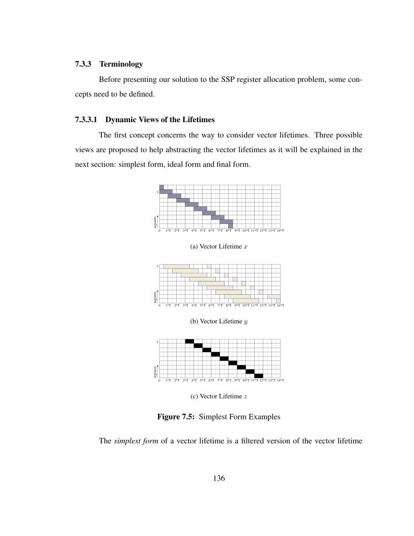
7.3.3 Terminology

Before presenting our solution to the SSP register allocation problem, some con-

cepts need to be defined.

7.3.3.1 Dynamic Views of the Lifetimes

The first concept concerns the way to consider vector lifetimes. Three possible

views are proposed to help abstracting the vector lifetimes as it will be explained in the

next section: simplest form, ideal form and final form.

0 2*T 3*T 4*T 5*T 6*T 7*T 8*T 9*T1*T 11*T 12*T 13*T 14*T10*T

regi

ster

s

x

(a) Vector Lifetime x

regi

ster

s

0 2*T 3*T 4*T 5*T 6*T 7*T 8*T 9*T1*T 11*T 12*T 13*T 14*T10*T

y

(b) Vector Lifetime y

0 2*T 3*T 4*T 5*T 6*T 7*T 8*T 9*T1*T 11*T 12*T 13*T 14*T10*T

regi

ster

s

z

(c) Vector Lifetime z

Figure 7.5: Simplest Form Examples

The simplest form of a vector lifetime is a filtered version of the vector lifetime

136

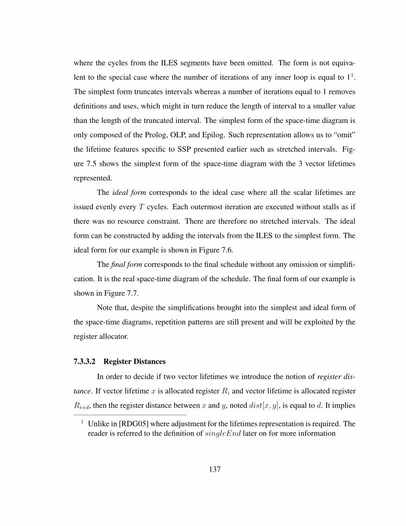
where the cycles from the ILES segments have been omitted. The form is not equiva-

lent to the special case where the number of iterations of any inner loop is equal to 11.

The simplest form truncates intervals whereas a number of iterations equal to 1 removes

definitions and uses, which might in turn reduce the length of interval to a smaller value

than the length of the truncated interval. The simplest form of the space-time diagram is

only composed of the Prolog, OLP, and Epilog. Such representation allows us to “omit”

the lifetime features specific to SSP presented earlier such as stretched intervals. Fig-

ure 7.5 shows the simplest form of the space-time diagram with the 3 vector lifetimes

represented.

The ideal form corresponds to the ideal case where all the scalar lifetimes are

issued evenly every T cycles. Each outermost iteration are executed without stalls as if

there was no resource constraint. There are therefore no stretched intervals. The ideal

form can be constructed by adding the intervals from the ILES to the simplest form. The

ideal form for our example is shown in Figure 7.6.

The final form corresponds to the final schedule without any omission or simplifi-

cation. It is the real space-time diagram of the schedule. The final form of our example is


Note that, despite the simplifications brought into the simplest and ideal form of

the space-time diagrams, repetition patterns are still present and will be exploited by the

register allocator.

7.3.3.2 Register Distances

In order to decide if two vector lifetimes we introduce the notion of register dis-

tance. If vector lifetime x is allocated register Ri and vector lifetime is allocated register

Ri+d, then the register distance between x and y, noted dist[x, y], is equal to d. It implies

1 Unlike in [RDG05] where adjustment for the lifetimes representation is required. Thereader is referred to the definition of singleEnd later on for more information

137

0 2*T 3*T 4*T 5*T 6*T 7*T 8*T 9*T1*T 11*T 12*T 13*T 14*T 15*T 16*T 17*T 20*T19*T18*T10*T

regi

ster

s

x


0 2*T 3*T 4*T 5*T 6*T 7*T 8*T 9*T1*T 11*T 12*T 13*T 14*T 18*T 20*T19*T15*T 16*T 17*T10*T

regi

ster

s

y


0 2*T 3*T 4*T 5*T 6*T 7*T 8*T 9*T1*T 11*T 12*T 13*T 14*T 15*T 16*T 17*T 18*T 19*T10*T

regi

ster

s

20*T

z


Figure 7.6: Ideal Form Examples

that vector lifetime x is below and to the left of vector lifetime y in the space-time dia-

gram. If y is below x, then the distance is noted dist[y, x]. Figure 7.8 shows an example.

The notion of register distance is only valid with the final form of the space-time diagram.

For the purpose of our algorithms we define two minimum legal register distances.

The conservative distance is the minimum register distance between two vector lifetimes

x and y, noted cons[x, y], so that they do not overlap or interleave. In other words, it is the

minimum register distance between vector lifetimes so that their convex envelops do not

overlap. Figure 7.9 shows our three lifetimes on the space-time cylinder where z is above

y above x. We have dist[y, z]=cons[y, z]=3, and dist[x, y]=cons[x, y]=1. None of the

vector lifetimes overlap and intervals from different vector lifetimes are not interleaved.

138

0 2*T 3*T 4*T 5*T 6*T 7*T 8*T 9*T1*T 11*T 12*T 13*T 14*T 15*T 16*T 17*T 20*T19*T18*T 21*T 22*T 23*T 24*T 25*T 26*T 27*T 28*T 29*T 30*T 31*T 32*T10*T

regi

ster

sx



regi

ster

s

y


regi

ster

s


z


Figure 7.7: Final Form Examples

The register requirement for this solution is equal to the circumference of the cylinder, 9.

The aggressive distance is the minimum register distance between two vector life-

times x and y, noted aggr[x, y], so that they do not overlap. Unlike the conservative

distance, interleaving is allowed. As proved by the experiments, the aggressive distance

will allow for a more fine-grain register allocation resulting in a lower requirement in

registers. Figure 7.10 presents an optimal solution with 7 registers where the distance be-

tween the vector lifetimes is equal to the aggressive distance: dist[y, z]=aggr[y, z]=1, and

dist[x, y]=aggr[x, y]=1. With the aggressive solution the intervals from vector lifetimes

are interleaved.

139

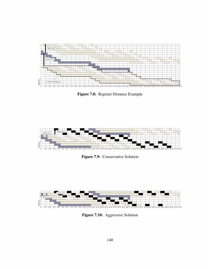
regi

ster

s


x

y

y

dist[x,y]=4

dist[y,x]=6

convex envelop of y

Figure 7.8: Register Distance Example

regi

ster

s


xy

zdist[y,z]=3

dist[x,y]=1

Figure 7.9: Conservative Solution

regi

ster

s


xyz

dist[x,y]=1

dist[y,z]=1

Figure 7.10: Aggressive Solution

140

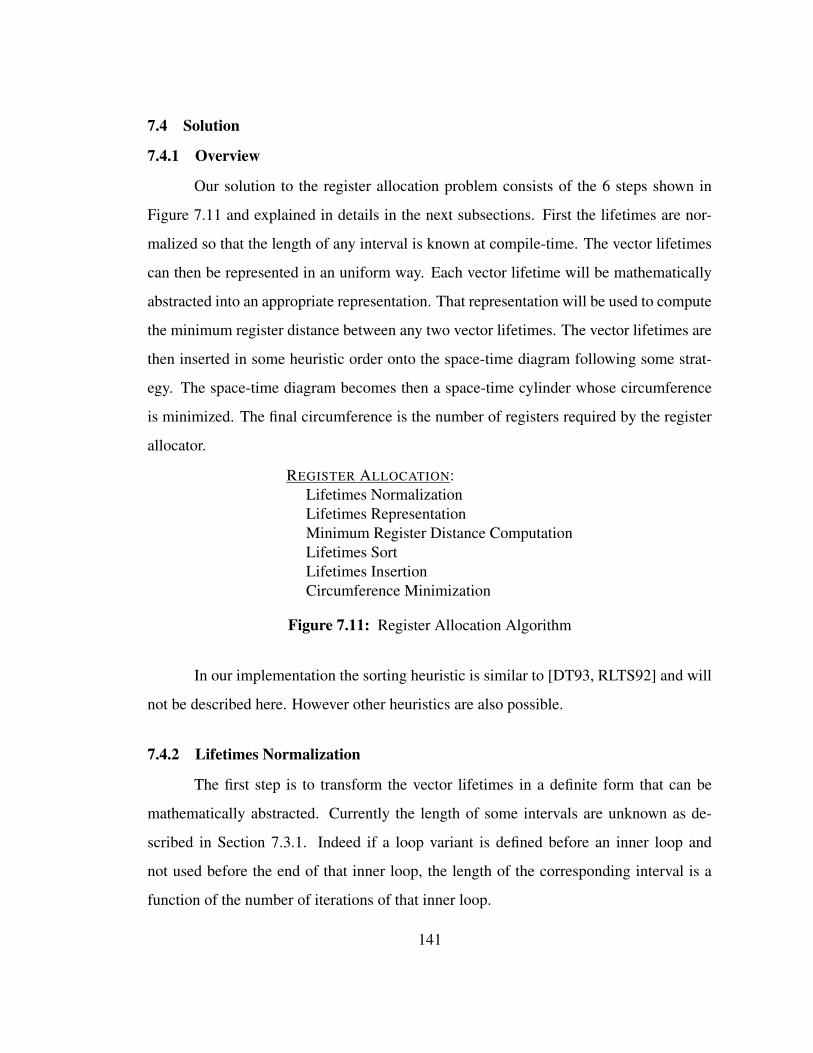
7.4 Solution

7.4.1 Overview

Our solution to the register allocation problem consists of the 6 steps shown in

Figure 7.11 and explained in details in the next subsections. First the lifetimes are nor-

malized so that the length of any interval is known at compile-time. The vector lifetimes

can then be represented in an uniform way. Each vector lifetime will be mathematically

abstracted into an appropriate representation. That representation will be used to compute

the minimum register distance between any two vector lifetimes. The vector lifetimes are

then inserted in some heuristic order onto the space-time diagram following some strat-

egy. The space-time diagram becomes then a space-time cylinder whose circumference

is minimized. The final circumference is the number of registers required by the register

allocator.

REGISTER ALLOCATION:Lifetimes NormalizationLifetimes RepresentationMinimum Register Distance ComputationLifetimes SortLifetimes InsertionCircumference Minimization

Figure 7.11: Register Allocation Algorithm

In our implementation the sorting heuristic is similar to [DT93, RLTS92] and will

not be described here. However other heuristics are also possible.

7.4.2 Lifetimes Normalization

The first step is to transform the vector lifetimes in a definite form that can be

mathematically abstracted. Currently the length of some intervals are unknown as de-

scribed in Section 7.3.1. Indeed if a loop variant is defined before an inner loop and

not used before the end of that inner loop, the length of the corresponding interval is a

function of the number of iterations of that inner loop.

141

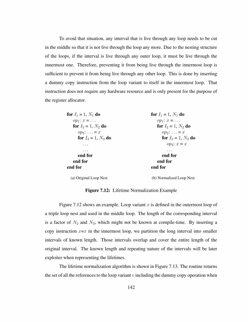
To avoid that situation, any interval that is live through any loop needs to be cut

in the middle so that it is not live through the loop any more. Due to the nesting structure

of the loops, if the interval is live through any outer loop, it must be live through the

innermost one. Therefore, preventing it from being live through the innermost loop is

sufficient to prevent it from being live through any other loop. This is done by inserting

a dummy copy instruction from the loop variant to itself in the innermost loop. That

instruction does not require any hardware resource and is only present for the purpose of

the register allocator.

for I1 = 1, N1 doop1: x = . . .for I2 = 1, N2 doop2: . . . = xfor I3 = 1, N3 do. . .. . .

end forend for

end for

(a) Original Loop Nest

for I1 = 1, N1 doop1: x = . . .for I2 = 1, N2 doop2: . . . = xfor I3 = 1, N3 doop3: x = x. . .

end forend for

end for

(b) Normalized Loop Nest

Figure 7.12: Lifetime Normalization Example

Figure 7.12 shows an example. Loop variant x is defined in the outermost loop of

a triple loop nest and used in the middle loop. The length of the corresponding interval

is a factor of N2 and N3, which might not be known at compile-time. By inserting a

copy instruction x=x in the innermost loop, we partition the long interval into smaller

intervals of known length. Those intervals overlap and cover the entire length of the

original interval. The known length and repeating nature of the intervals will be later

exploiter when representing the lifetimes.

The lifetime normalization algorithm is shown in Figure 7.13. The routine returns

the set of all the references to the loop variant v including the dummy copy operation when

142

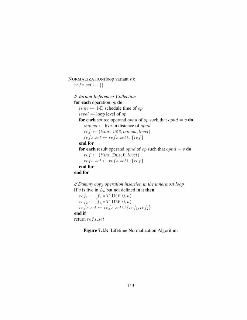
NORMALIZATION(loop variant v):refs set← {}

// Variant References Collectionfor each operation op dotime← 1-D schedule time of oplevel← loop level of opfor each source operand opnd of op such that opnd = v doomega← live-in distance of opndref ← (time,USE, omega, level)refs set← refs set ∪ {ref}

end forfor each result operand opnd of op such that opnd = v doref ← (time,DEF, 0, level)refs set← refs set ∪ {ref}

end forend for

// Dummy copy operation insertion in the innermost loopif v is live in Ln but not defined in it thenref1 ← (fn ∗ T,USE, 0, n)ref2 ← (fn ∗ T,DEF, 0, n)refs set← refs set ∪ {ref1, ref2}

end ifreturn refs set

Figure 7.13: Lifetime Normalization Algorithm

143

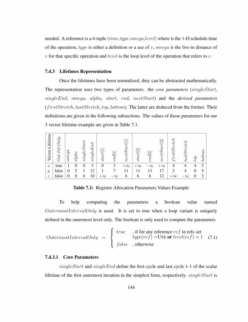
needed. A reference is a 4-tuple (time,type,omega,level) where is the 1-D schedule time

of the operation, type is either a definition or a use of v, omega is the live-in distance of

v for that specific operation and level is the loop level of the operation that refers to v.

7.4.3 Lifetimes Representation

Once the lifetimes have been normalized, they can be abstracted mathematically.

The representation uses two types of parameters: the core parameters (singleStart,

singleEnd, omega, alpha, start, end, nextStart) and the derived parameters

(firstStretch, lastStretch, top, bottom). The latter are deduced from the former. Their

definitions are given in the following subsections. The values of those parameters for our

3 vector lifetime example are given in Table 7.1.

Vec

torL

ifet

ime

Out.Int.Only

omega

alpha

singleStart

singleEnd

start

[1]

end[1

]

nextStart

[1]

start

[2]

end[2

]

nextStart

[2]

firstStretch

lastStretch

top

bottom

x true 1 0 0 3 0 3 +∞ +∞ −∞ +∞ 4 4 4 5y false 0 2 1 12 1 7 11 11 13 17 3 4 0 5z false 0 0 6 10 +∞ −∞ 6 6 8 12 +∞ −∞ 0 3

Table 7.1: Register Allocation Parameters Values Example

To help computing the parameters a boolean value named

OutermostIntervalOnly is used. It is set to true when a loop variant is uniquely

defined in the outermost level only. The boolean is only used to compute the parameters

OutermostIntervalOnly =

true , if for any reference ref in refs settype(ref) =USE or level(ref) = 1

false , otherwise(7.1)

7.4.3.1 Core Parameters

singleStart and singleEnd define the first cycle and last cycle + 1 of the scalar

lifetime of the first outermost iteration in the simplest form, respectively. singleStart is

144

therefore equal to the cycle of the first definition of that loop variant in 1-D schedule and

singleEnd is the cycle+1 of the last reference in that same schedule, to which we add the

omega distance omega∗T 2. If the last reference is a definition before the first occurrence

of the ILES (not represented in the simplest form) and a use for that loop variant is present

in the ILES, then the loop variant is still live until the start cycle of that ILES. singleEnd

is then start cycle of the first ILES, namely ln ∗ T .

singleStart = min

{time(ref),

∀ref ∈ refs set such that type(ref) =DEF

}(7.2)

singleEnd = max

{time(ref) + 1 + omega(ref) ∗ T ,

∀ref ∈refs set ∪ {(adjustment,USE, 0, 1)}

}(7.3)

where,

adjustment =

−∞ , if OutermostIntervalOnly

ln ∗ T , otherwise

Omega and alpha are the maximum number of live-in and live-out values, respec-

tively, for the loop variant. Omega can be computed from the references whereas alpha

is assumed to have been computed by an earlier phase of the compiler.

omega = max{omega(r),∀ref ∈ refsset} (7.4)

Start[i] is the issue time of the definition of the variant at level i, which is equal

to its 1-D schedule time. End[i] is 1 + the latest issue time of all possible uses of the

definition. If the definition at level i has no use, end[i] is the 1-D schedule time of the

definition + 1. The variant is live for the duration of the definition. If there is no definition

of the variant at level i, then start[i] and end[i] are set to +∞ and −∞, respectively.

The arbitrary choice is compatible with the subsequent distance computation because we

would have end[i]− start[i] < 0.

2 In [RDG05], singleEnd needs to be adjusted because the simplest form was defineddifferently. Here the adjustment is directly included in the definition of singleEnd

145

The computation of start[i] is straightforward. However end[i] is harder to com-

pute. Let uses(d) be the set of uses of a definition d. An operation u is a use of a definition

d if the control-flow can reach u from d without encountering any redefinition of the loop

variant. Let loopbackOffset(d, u) be the offset due to the execution of a back loop edge.

It corresponds to the execution time of one iteration of the shallowest loop traversed by

the control-flow while flowing from d to u. If d is the definition of the loop variant at level

i, we have:

start[i] =

time(d) , if d is defined

+∞ , otherwise(7.5)

end[i] =

max

time(u) + 1 + omega(u) ∗ T+loopbackOffset(d, u), ∀u ∈ uses(d)

, if d is defined

and uses(d) 6= {}

time(d) + 1 , if d is definedand uses(d) = {}

−∞ , otherwise

(7.6)

7.4.3.2 Derived Parameters

The derived parameters characterize the stretched intervals of the vector lifetimes.

Because the length of a stretched intervals is relative to the number of iterations of the

inner loops, it is unknown at compile-time and cannot be abstracted horizontally in the

space-time diagram as it was done for the core parameters. Instead, the vertical axis,

i.e. the number of registers, is used. There are 4 derived parameters.

firstStretch and lastStretch are the iteration indexes of the first and last

stretched intervals in the first ILES segment. If there is no stretched interval, then they

are set to +∞ and −∞, respectively. Let us consider the first ILES segment. An interval

at iteration index x ≥ 0 at level i is stretched if its definition appears before the first cycle

of the first ILES, and if its last use appears at that same first cycle or later in a different

iteration group. If span = omega when i = 1 and 0 otherwise, those conditions can be

146

formulated as:

start[i] + x ∗ T < ln ∗ T

end[i] + x ∗ T > ln ∗ T

x+ span ≥ Sn

Let first and last be the smallest and largest x values that satisfy the above in-

equalities. Then we have:

first = min∀i∈[1,n]

{max

(0, Sn − span, ln −

⌊end[i]− 1

T

⌋)}

last = max∀i∈[1,n]

{ln −

⌈start[i] + 1

T

⌉}

If first > last, then there is no stretched interval. Also, for single loops (n =

1), there never is any stretched interval. We then have the mathematical definitions of

firstStretch and lastStretch:

firstStretch =

+∞ if n = 1 or first > last

first otherwise(7.7)

lastStretch =

−∞ if n = 1 or first > last

last otherwise(7.8)

The last two parameters characterize the height of the ILES segment. Top is the

iteration index of the top intervals in the ILES and bottom is the iteration index plus one

of the intervals at the bottom of the ILES. If there is no interval in the ILES, then top

and bottom are set to +∞ and −∞, respectively. Two cases arise. If the loop variant is

uniquely defined in the outermost level (outermostIntervalOnly), then the ILES seg-

ment is only made of stretched intervals. Otherwise it is made of Sn intervals from the

147

iteration group being executed and of the stretched intervals of the other iteration groups.

Therefore:

top =

firstStretch if outermostIntervalOnly

0 otherwise(7.9)

bottom =

lastStretch+ 1 if outermostIntervalOnly

max(Sn, lastStretch+ 1) otherwise(7.10)

7.4.4 Minimum Register Distance Computation

Using our representation of the vector lifetimes, we can now compute the min-

imum register distance between any two vector lifetimes. Two minimum distances are

proposed: conservative and aggressive.

7.4.4.1 Conservative Distance

The conservative distance considers the concave envelope of the vector lifetimes

when evaluating the minimum register distance between vector lifetimes. Let us con-

sider two vector lifetimes x and y that have been allocated registers Rx and Ry respec-

tively. We assume that y appears on the right of x in the space-time diagram and we note

d=dist[x, y]=Ry −Rx. Four constraints must be taken into account.

regi

ster

s

0 2*T 3*T 4*T 5*T 6*T 7*T 8*T 9*T1*T 11*T 12*T 13*T 14*T10*T

Rx

Ry

d

singleStart(y)

singleEnd(x)

T

singleStart(y) + d * T − singleEnd(x)

Figure 7.14: Conservative Distance: Wands

148

First the wand of y must be above and to the right of x without overlapping parts

of x. Because in the simplest form the wand is composed of N1 identical scalar life-

times, which are issued every T cycles, one must only ensure that no conflict exists

for the the first scalar lifetime of x for instance. The end of the first scalar lifetime of

x is singleEnd(x). The beginning of the scalar lifetime sharing the same register is

singleStart(y) + (Ry − Rx) ∗ T . There is therefore no conflict if the distance between

the two is positive, i.e. singleStart(y) + d ∗ T − singleEnd(x) ≤ 0.

Second the leading blade of vector lifetime y must not overlap with vector lifetime

x. If omega(y) = 0, then there is no leading blade and therefore no problem. Otherwise,

since leading blades always start from cycle 0, the last scalar lifetime of the leading blade

of y must be above any scalar lifetime of x. The first scalar lifetime of x is assigned to

Rx + omega(x). The last scalar lifetime of the leading blade of y is assigned Ry + 1.

Therefore we must have Ry > Rx + omega(x), i.e. d > omega(x).

Third the trailing blades should not overlap. Using a symmetrical reasoning to the

leading blades issues, we obtain the last condition: d > alpha(x).

Last, the ILES segments must not overlap in the final form of the space-time

diagram. The bottom of vector lifetime y must be above the top of vector lifetime x,

i.e. Ry − bottom(y) ≥ Rx − top(x).

If those four conditions are satisfied, then the vector lifetimes of x and y do not

overlap. The minimum value of d satisfying those conditions is the minimum conservative

distance between x and y. There is no maximum. Those results are summarized in

Figure 7.15.

An example is shown in Figure 7.16 for vector lifetimes x and y. We have

singleEnd(x) = 3 and singleStart(y) = 1, therefore d1 = 1. omega(y) = 0 and

alpha(x) = 0, therefore d2 = d3 = 0. Because Bottom(y) = 5 and top(x) = 4, we have

d4 = 1 and cons[x, y] = [1,+∞[. Once Rx has been set, Ry can legally take any value

between Rx + 1 and above. In the figure, Ry takes the minimum legal value of Rx + 1.

149

d1 =

⌈singleEnd(x)− singleStart(y)

T

⌉

d2 =

{0 , if omega(y) = 0omega(x) , otherwise

d3 =

{0 , if alpha(x) = 0alpha(x) , otherwise

d4 = bottom(y)− top(x)

=⇒ cons[x, y] = [max(d1, d2, d3, d4),+∞[

Figure 7.15: Conservative Distance Computation

regi

ster

s

0 2*T 3*T 4*T 5*T 6*T 7*T 8*T 9*T1*T 11*T 12*T 13*T 14*T10*T

cons

[x,y

]

RxRy

illeg

al

Figure 7.16: Conservative Distance Example

150

7.4.4.2 Aggressive Distance

With the aggressive distance we try to take advantage of the space between inter-

vals to interleave vector lifetimes. For this the simplest form is not sufficient anymore and

one must look at the ideal and final form of the space-time diagrams. Several constraints

must be taken into account.

First, given a loop level i, the intervals at that level must interleave without over-

lapping. In the ideal form (stretched intervals will be dealt with later with the final form),

we consider the intervals from vector lifetimes x and y at level i. The end (start, respec-

tively) of the intervals of y must be before the start (after the end) of the intervals of x.

This is abstracted as starty[i] + d ∗ T ≥ endx[i] and endy[i] + d ∗ T ≤ nextStartx[i],

respectively. If there is no interval for y at level i (starty[i] = +∞ and endy[i] = −∞,

we still need to ensure that the next interval of y at the next loop level does not overlap

with an interval of x at level i, i.e. nextStarty[i] + d ∗ T ≥ endx[i]. Those conditions

give us a lower lx,y[i] and upper bound ux,y[i] for the register distance between the two

vector lifetimes so that interleaving is allowed:

lx,y[i] =

⌈endx[i]−nextStarty [i]

T

⌉, if starty[i] = +∞ and endy[i] = −∞

⌈endx[i]−starty [i]

T

⌉, otherwise

ux,y[i] =

⌊nextStartx[i]− endy[i]

T

⌋

The intersection of the segments [lx,y[i], ux,y[i]] over all the loop levels i is the

range of register distances from y to x in the space-time diagram so that the intervals are

interleaved without overlapping, stretched intervals excluded. The lower and upper bound

of that intersection are given by d5 and d6, respectively, in Figure 7.17.

Then we consider the final form and take into account the stretched intervals. The

stretched intervals of y should be above the stretched intervals of x if any, and below the

151

non-stretched intervals of x in the ILES. We then have the inequalities below that will be

translated into d7 and d8 in Figure 7.17.

Ry − bottom(y) ≥ Rx − firstStretch(x)

Ry − firstStretch(y) ≤ Rx − Sn , if not outermostIntervalOnly(x)

The final segment intl[x, y] is the range of legal distances between vector lifetime

x and vector lifetime y so that the vector lifetimes are interleaved without overlapping. If

empty, interleaving is not possible. To obtain the full range of legal distances, the union

of intl[x, y] and the conservative range cons[x, y] must be made. The result is the range

of legal aggressive distances between x and y. The summary of the computation of the

aggressive distance is shown in Figure 7.17 3.

d5 = max∀i∈[1,n]

{lx,y[i]}

d6 = min∀i∈[1,n]

{ux,y[i]}

d7 = bottom(y)− firstStretch(x)

d8 =

{+∞ , if outermostintervalonly(x)firstStretch(x)− Sn , otherwise

=⇒ intl[x, y] = [max(d5, d7),min(d6, d8)]

aggr[x, y] = cons[x, y] ∪ intl[x, y]

Figure 7.17: Aggressive Distance Computation

In Figure 7.18, we show how the aggressive distance is computed between vector

lifetimes z and y. Using the ideal form, the end of the interval of z in the outermost level,

noted interval 1, and the start of the first outermost interval of y, noted interval 2, do not

3 In [RDG05] there are two extra terms d9 and d10. Because those terms were redun-dant with d2 and d3, they are not used anymore.

152

overlap if dist[z, y] ≥ lz,y[1] = −∞. Because interval 1 does not actually exist, its end

was set to−infty. Similarly intervals 2 and 3 do not overlap if the distance between z and

y is greater than uz,y[1] = −1. For the innermost level, interval 4 must start after the end

of interval 3 and lz,y[2] = −1. And interval 4 must end before the next innermost interval

(5) and uz,y[2] = −1. Therefore d5 = d6 = −1, which means that if dist[z, y] 6= −1, the

vector lifetimes either overlap or are not interleaved.

0 2*T 3*T 4*T 5*T 6*T 7*T 8*T 9*T1*T 11*T 12*T 13*T 14*T 18*T 20*T19*T15*T 16*T 17*T10*T

zy1 2 3 4 5

(a) Ideal Form


yz

6

78

9

(b) Final Form

Figure 7.18: Aggressive Distance Example

Using the final form in Figure 7.18(b), the constraints of the stretched intervals are

taken into account. For the interleaving to be legal, the first stretched interval of y, interval

7 in the figure, must be below the non-stretched intervals of z, represented by interval 6.

Also the last stretched intervals of y, interval 8, must be above the first stretched interval of

z (non-existing in this example, but still represented as interval 9). Those two conditions

lead to d7 = −∞ and d8 = 0. Finally we obtain intl[z, y] = [−1,−1].

153

7.4.4.3 Property

As for the schedule function, the register distance formulas subsume single loops

as a special case.

Property 7.1 Given a single loop L and two vector lifetimes x and y of L, cons[x, y] =

aggr[x, y] = [l,+∞[ where l is the minimum register distance calculated using Rau’s

register allocation for single loops [RLTS92].

Proof. In a single loop a vector lifetime is made of a single interval per scalar lifetime

and start[1] = singleStart, end[1] = singleEnd, and nextStart[1] = +∞. Because

there is no ILES segment, we also have firstStretch = +∞, lastStretch = −∞,

top = +∞, and bottom = −∞. We have to prove that both the conservative and the

aggressive distances are equal to the distance defined by Rau.

For the conservative distance, because bottom = −∞, we have d4 = −∞ and

cons[x, y] can be rewritten as [max(d1, d2, d3),+∞[. The definition of the conservative

distance is then identical to the definition of the minimum register distance in Rau’s algo-

rithm.

For the aggressive distance, d7 and d8 are set to −∞ and +∞, respectively. Be-

cause nextStart[1] is equal to +∞, we have ux,y[1] = +∞, and d6 = +∞. Finally we

obtain:

lx,y[1] =

⌈endx[i]− starty[i]

T

⌉=

⌈singleEndx − singleStarty

T

⌉= d1

Therefore intl[x, y] = [d1,+∞[ and aggr[x, y] = cons[x, y]. �

7.4.5 Lifetimes Insertion

After being sorted, the vector lifetimes are inserted onto the surface of a space-time

cylinder of circumference equal to R, the number of physical rotating registers available

on the target architecture. It would be possible to insert lifetimes on a space-time cylinder

with an infinite circumference. However, because the number of physical registers is

154

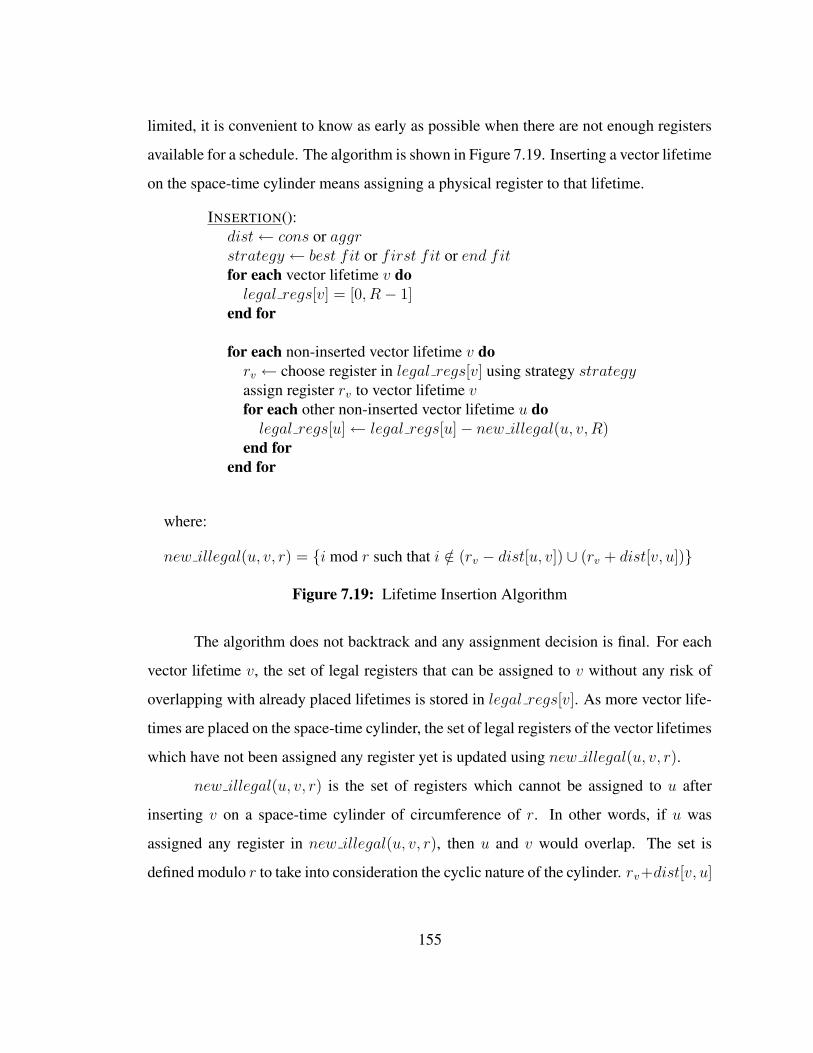
limited, it is convenient to know as early as possible when there are not enough registers

available for a schedule. The algorithm is shown in Figure 7.19. Inserting a vector lifetime

on the space-time cylinder means assigning a physical register to that lifetime.

INSERTION():dist← cons or aggrstrategy ← best fit or first fit or end fitfor each vector lifetime v dolegal regs[v] = [0, R− 1]

end for

for each non-inserted vector lifetime v dorv ← choose register in legal regs[v] using strategy strategyassign register rv to vector lifetime vfor each other non-inserted vector lifetime u dolegal regs[u]← legal regs[u]− new illegal(u, v, R)

end forend for

where:

new illegal(u, v, r) = {i mod r such that i /∈ (rv − dist[u, v]) ∪ (rv + dist[v, u])}

Figure 7.19: Lifetime Insertion Algorithm

The algorithm does not backtrack and any assignment decision is final. For each

vector lifetime v, the set of legal registers that can be assigned to v without any risk of

overlapping with already placed lifetimes is stored in legal regs[v]. As more vector life-

times are placed on the space-time cylinder, the set of legal registers of the vector lifetimes

which have not been assigned any register yet is updated using new illegal(u, v, r).

new illegal(u, v, r) is the set of registers which cannot be assigned to u after

inserting v on a space-time cylinder of circumference of r. In other words, if u was

assigned any register in new illegal(u, v, r), then u and v would overlap. The set is

defined modulo r to take into consideration the cyclic nature of the cylinder. rv+dist[v, u]

155

represents the set of registers that can be allocated to u without any conflict with v if u is

to be inserted above v. Otherwise the set of legal registers is given by rv − dist[u, v].

axis of the space−time cylinder

vr

legal_regs[u] withaggressive distanceconservative distance

legal_regs[u] with

r v + cons[v,u]

r v − cons[u,v]

r v − intl[u,v]

+ intl[v,u]r v

Figure 7.20: Lifetime Insertion Example

Figure 7.20 shows the legal regs set of vector lifetime u after assigning register

rv to vector lifetime v. If the aggressive distance is used, the set of legal registers is larger.

7.4.6 Circumference Minimization

At this point all the vector lifetimes have been placed on the surface of space-time

cylinder of circumference equal to the number of physical registers available in the target

architecture, R. The next step is to minimize that circumference to minimize register

usage. The algorithm is shown in Figure 7.21.

First the registers assigned to the vector lifetimes are reindexed to start at index 0.

Then the circumference of the space-time cylinder is initialized a tight lower bound: the

difference between the lowest and highest register used. From there, the circumference

is tested. If any vector lifetime overlaps itself and another vector lifetime, the circumfer-

ence is incremented by one. As soon as no overlapping is detected the algorithm stops.

The current circumference is the minimum number of rotating registers required by the

156

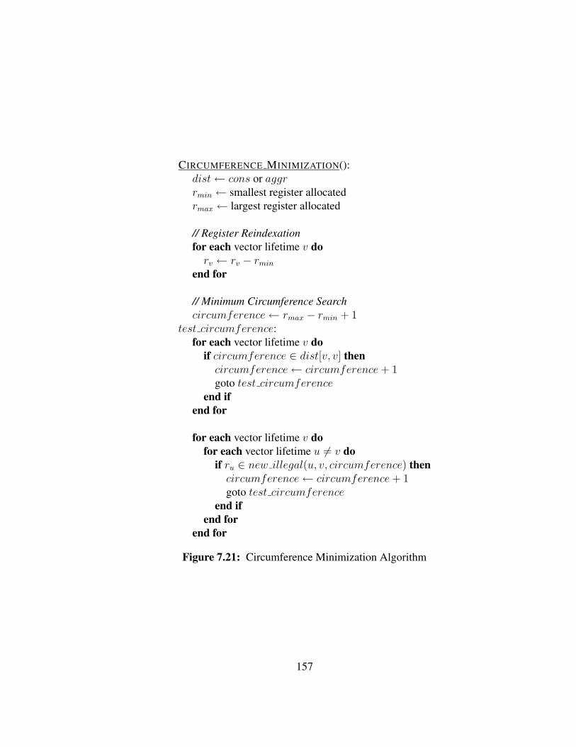
CIRCUMFERENCE MINIMIZATION():dist← cons or aggrrmin ← smallest register allocatedrmax ← largest register allocated

// Register Reindexationfor each vector lifetime v dorv ← rv − rmin

end for

// Minimum Circumference Searchcircumference← rmax − rmin + 1

test circumference:for each vector lifetime v do

if circumference ∈ dist[v, v] thencircumference← circumference+ 1goto test circumference

end ifend for

for each vector lifetime v dofor each vector lifetime u 6= v do

if ru ∈ new illegal(u, v, circumference) thencircumference← circumference+ 1goto test circumference

end ifend for

end for

Figure 7.21: Circumference Minimization Algorithm

157

schedule. Because we already know that no overlapping occurs with a circumference of

R, the algorithm is guaranteed to converge.

7.4.7 Time Complexity

Let nv be the number of vector lifetimes and no the number of operations in the

schedule. The lifetime normalization and representation algorithms have a time complex-

ity of O(no) per loop variant and an overall complexity of O(no ∗ nv). The time spent

computing distances for all the pair of loop variants is O(n2v). Sorting can be done in

O(n2v). The vector lifetime insertion uses the same strategies as in [RLTS92], and there-

fore run in O(n2v) for first and end fit, and O(n3

v) for best fit. Finally the circumference

minimization runs in O(n2v). Overall the register allocation algorithms have a time com-

plexity of O(n2v + nv ∗ no) with first or end fit and O(n3

v + nv ∗ no) with best fit.


The register allocation method was implemented, alongside with the rest of the

SSP framework, in the ORC 2.1 compiler. The input of the register allocator is the kernel

produced by the scheduler (Chapter 5) and the output is a register-allocated kernel to be

sent to the code generator (Chapter 8).


The vector lifetimes were sorted in increasing order by adjacency. Ties are bro-

ken using singleStart, then adjustedSingleEnd modulo T . The adjacency between

two vector lifetimes v and u represents the number of cycles a register is idle. It is de-

fined as singleStart(u) − singleEnd(v) + d3(v, u) ∗ T . The heuristic is an extension

to the (adjacency, start time) heuristic used in the traditional register allocation for single

loops [RLTS92].

Seven different strategies were used for the insertion of vector lifetimes on the

space-time cylinder. The first, referred to as Simple, ignores the specific shape of a

158

vector lifetime u and exclusively allocates to it S+omega(u) physical registers, which is

the maximum number of instances of a loop variant that can be live simultaneously in the

final schedule (S is the number of stages in the SSP kernel). The two register distances,

conservative and aggressive, were tested combined with the three strategies introduced

in Section 7.2: first fit, best fit, and end fit. The 6 combinations are named Cons-

First, ConsBest, ConsEnd, AggrFirst, AggrBest, and AggrEnd, respectively. Besides,

the register pressure of the schedule, MaxLive (Section 6), was measured for comparison.

Depth 1 2 3 4 5Number 127 108 68 33 12

Table 7.2: Depth of the Tested Loop Nests

A total of 134 loop nests were gathered from NAS, Livermore and SPEC2000

benchmark suites. To test the register pressure related with different levels, SSP was ap-

plied to each feasible level, leading to a total of 348 loop levels tested. Note that even

for the same variant in the same source code, software pipelining of two different levels

results in completely different vector lifetimes. The distribution of the depths of the loop

nests is shown in Table 7.2. The space-time cylinder was assumed a maximum circumfer-

ence of 1024 registers. When the number of registers allocated did not exceed 96 rotating

integer and floating-point registers, the total rotating registers in Itanium architecture, the

parallelized loop nest was run on an Itanium2 machine, and correctness was validated by

comparing its output with that of the same loop nest compiled with GCC or the original

ORC 2.1 binary.

Overall, 60% of the loops have 47 operations or less , but 12% of the loops have

more than 200. 64% of the loops have an II of less that 10 cycles, and 8.4% of them have

an II larger than 40 cycles. Note that, because a smaller II may be related to a higher

number of stages, it tends to increase the register pressure. 80% of the loops have 56

integer loop variants or less and the maximum is 174. For floating-point loop variants,

159

80% of the loops has less than 45 with a maximum of 96. The total number of stages

never exceeds 11 and the number of live-in values never goes above 7.

7.5.2 Register Requirements

The register requirements for each distance-strategy combination are shown in

Figure 7.22. The curves are cumulative distribution curves. Each one indicates the per-

centage of loop nests whose register-allocated schedule requires a given number of regis-

ters. The curves are surrounded by the register requirement curves of Maxlive and Simple.

Those two curves are the lowest and upper bound, respectively. The Maxlive curve rep-

resents the minimum register requirement that would be achieved by an ideal register

allocator. As such, the closer a curve is to the Maxlive curve, the better is the register

allocation solution. The maximum number of available physical rotating registers, 96, is

represented by a vertical bar.

At a first look, we can distinguish 3 groups of curves. The first group includes the

curves from the 3 combinations using the conservative distance. It is the lowest group on

both graphs. The second group includes the curves from the aggressive distance solutions,

combined with best or first fit. It is the highest group on both graphs. The two curves are

almost identical. The last group is composed of a unique curve: the aggressive distance

solution combined with the end fit strategy. It is the curve in the middle.

Using the Simple register allocation scheme, only 30% of the loop nests requires

96 registers or less. Using the conservative distance, the rate increases to 53%, and then

to almost 92% with the aggressive distance. Overall the proposed register allocation

allows 76.5% of the loop nests to be compiled with 96 registers or less. This result

confirms the importance of exploiting the specific patterns of the vector lifetimes in SSP

schedules. A deeper analysis of the register allocation solutions revealed in some cases

up to 4 vector lifetimes interleaved with each other when the aggressive distance is used.

That phenomenon was not uncommon.

160

100%

80%

60%

40%

20%

100 200 300

Perc

enta

ge o

f Loo

p N

ests

Number of Registers Required

Maxlive

Simple

AggrBestAggrFirstAggrEndConsBestConsFirstConsEnd

(a) Integer Registers

100%

80%

60%

40%

20%

100 200 300

Perc

enta

ge o

f Loo

p N

ests

Number of Registers Required

Maxlive

Simple

AggrBestAggrFirstAggrEndConsBestConsFirstConsEnd

(b) Floating-Point Registers

Figure 7.22: Cumulative Distribution of the Register Requirements for the Loop Nestsof Depth 2 or Higher

161

Moreover the register requirement curves of the register allocation solutions us-

ing the aggressive distance combined with first or best fit appear extremely close to the

Maxlive results. Considering the fact that Maxlive is not a tight lower bound, the result is

even more encouraging.

7.5.3 Lifetime Insertion Strategies

When the conservative distance is used, the vector lifetime insertion strategy is

not relevant. The three strategies are equivalent. However, with the aggressive distance,

the first and best fit strategies curves are indistinguishable and very close to the Maxlive

curve. Those two combinations succeeds in compiling 15% more loops than the aggres-

sive distance-end fit combination.

Nevertheless the advantage goes to the first fit strategy. When comparing the com-

pilation time of both the first and best fit strategies during the lifetime insertion step, it

appears that the first fit strategy is 3 orders of magnitude faster. The cubic factor in the

time complexity results plays a very important role.


Does a lower register requirement have a significant impact on run-time perfor-

mance? To measure it, we considered the 18 loop nests that had a register requirement

of 96 registers or less with the aggressive distance-first fit combination but more than 96

with the conservative distance-first fit combination. For those loop nests, the scheduler

was asked to recompute a schedule with a longer initiation interval. A direct consequence

is a reduced number of stages, and therefore a reduced number of lifetimes interfere and

number of registers required. The initiation interval is allowed to grow as large as neces-

sary to accommodate the 96 registers of the Itanium architecture.

Of the 18 loop nests that could not be register allocated, still 11 could not be

compiled with the Simple method and 5 with the conservative distance method. Indeed

the register pressure stops decreasing after a certain threshold, as already observed in

162

[LVA96]. For the other loop nests that could be compiled, the schedule was compared to

the original schedule. On average, the initiation interval of the Simple and conservative

distance solutions were 81% and 25% larger, respectively. And the execution time was

69% and 28% longer, respectively.

7.5.5 Single Loops

The algorithm was also applied to 127 single loops. As expected, the aggres-

sive and conservative distances were identical and the results matched the ones from

Rau [RLTS92]. The SSP register allocation subsumes single loops as a special case.

7.6 Related Work

The solution proposed in this chapter is currently register allocation proposed

for SSP schedules. Several other register allocation methods for modulo schedules ex-

ist [EDA94, EDA95, GAG94, WKEE94, NG93, HGAM92]. However they cannot be

applied to loop nests.

Existing methods for allocating registers for loop nests [HGAM92, CK91] are

extensions of the traditional graph coloring approach [Cha82] and do not aim at soft-

ware pipelining. However, lifetimes in a software pipelined loop have regular pat-

terns [RLTS92], which should be taken advantage of by an efficient register allocator.

Traditional software pipelining of loop nests [Lam88, MD01] centers around scheduling,

with little discussion on register allocation.

7.7 Conclusion

This chapter presented a software-pipelined loop nest register allocation scheme,

which can be applied to SSP kernels. Vector lifetimes of an SSP schedule have features

that do not have vector lifetimes in modulo scheduled single loops. A scalar lifetime is

composed of multiple intervals and multiple levels. Some intervals are stretched and are

163

not issued at regular intervals. The shape of a vector lifetime is not a convex polygon, but

a set of multiple intervals and holes between those.

The proposed solution takes advantages those holes to interleave the vector life-

times and reduce the overall register requirements of the SSP schedule. Thanks to an

accurate representation of the vector lifetimes, a range of legal distances between vec-

tor lifetimes is computed. A distance is deemed legal if the two vector lifetimes do not

interfere during the entire execution of the schedule. Using that information, the vector

lifetimes are placed one after the other on the surface of a space-time cylinder of circum-

ference equal to the number of physical registers of the target architecture. Afterward the

circumference is reduced as much as possible. The final result is the register allocated

kernel.

Experiments show that the method is very efficient and that interleaving vector

lifetimes is a sine qua non condition to reduce the register requirements of an SSP sched-

ule. The best heuristic (interleaving allowed and first fit strategy) allocates almost the

minimum number of registers required. If no interleaving is allowed, the quality of the

solutions quickly deteriorates. Results also show that, when the number of registers re-

quired exceeds the number of physical registers available in the target architecture, the

execution time of the schedule greatly suffers.

164

Chapter 8

CODE GENERATION

8.1 Introduction

This chapter describes the last step of the SSP framework described earlier in

Figure 3.6: the code generation. At this point in the framework, the kernel has been

computed and registers have been assigned to the loop variants of the loop nest. The

final step consists of generating the final schedule in assembly code using the the register-

allocated kernel.

The task is more complex than in the single loop case encountered by MS. The

code generator is now faced with different repeating patterns, one per loop level in the

loop nest. The overlapping live ranges must in turn also be taken into consideration and

require a separate level of register assignment for each loop level. Other issues related to

the loop overhead instructions management, the level separation constraint, the initializa-

tion/finalization of the SSP pipeline and the code size issue must also be solved. Those

issues are presented in more details in Section 8.2.3.

In this chapter we make the difference between code generation and code emis-

sion. The latter is a part of the former. Code emission is the process of writing assembly

instructions into the assembly file, whereas code generation is the process of computing

what should be written into the assembly file.

The rest of the chapter is organized as follows. First a more formal description

of the code generation problem is proposed where the different patterns and issues are

explained in details. Then our solution for the EPIC architecture is presented. Finally the

experimental results are analyzed before concluding.

165


8.2.1 Notations

Before giving a formal problem formulation some notations are needed. We

present here in details the different repeating patterns appearing in the final schedule.

Some examples have already been presented in Chapter 3.4. We make the difference be-

tween double loop nests and loop nests of depth 3 or higher. Single loops are generated

the same way as with MS and are not mentioned here.

8.2.1.1 Double Loop Nest

To describe the different phases and repeating patterns of the final schedule ap-

pearing in double loop nests, we use a different example from Section 3.4.2. The kernel

is shown below:

op1

op2op3

op4

op5

op6

abcde

Figure 8.1: Double Loop Nest Kernel

The corresponding final schedule is shown in Figure 8.2. Because the initiation

interval of each level is not relevant for our discussion, the number of cycles within each

stage is not represented. The final schedule can be partitioned into 3 different phases: the

outermost filling phase, the stable phase, and the outermost draining phase.

The stable phase is iterated as many times as needed and corresponds to the exe-

cution of the loop nest once the software-pipeline has been filled. It is composed of two

repeating patterns: the Outermost Loop Pattern (OLP) and the Innermost Loop Pattern

(ILP). The former issues the outermost iterations whereas the latter corresponds to the

execution of the innermost loop. The OLP is made of Sn consecutive copies of the entire

kernel. The ILP is also made of Sn copies of the kernel. However only the innermost

166

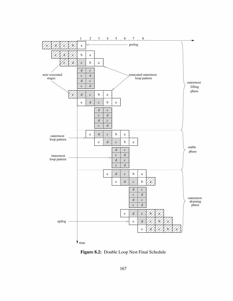
cddccddc

e d c b a

e d c b a

cddccddc

e d c b a

e d c b a

cddccddc

e d c b a

e d c b a

cddccddc

e

e d

e d c

e b a

c b a

e b a

b a

a

c

b

d

c

b a

d c

e d

d c

truncated outermostloop pattern

prolog

epilog

outermost

stablephase

outermostdraining

phase

fillingphase

loop patternoutermost

innermostloop pattern

non−executedstages

7654321 8

time

Figure 8.2: Double Loop Nest Final Schedule

167

stages are taken into consideration. Moreover, each new copy rotates the order of appear-

ance of the stages. In our example the first copy is made of stages c, then b, whereas the

second copy is made of stages b and c in that order.

The initialization phase corresponds to the part of the schedule before the stable

phase when the software-pipeline is being filled up. It is equivalent to the stable phase

from which we remove the stages from the non-existent previous outermost iterations

(i.e. iterations -1, -2, ...). It includes the Prolog and an alternated appearance of Truncated

OLPs and ILPs similar to the stable phase. The prolog can be seen as truncated OLPs

without the presence of ILPs in-between.

The conclusion phase is the symmetric opposite of the initialization phase and

corresponds to the part of the schedule after the stable when the software-pipeline is

being drained. It is equivalent to the stable phase from which we remove the non-existent

next outermost iterations (i.e. iterations N, N+1, ...). It includes an alternated appearance

of truncated OLPs and ILPs, and the Epilog. The epilog can also be seen as truncated

OLPs with the presence of ILPs in-between.

Therefore the entire final schedule can be derived from the kernel. More specif-

ically one only needs to be able to emit the prolog, the OLP (truncated or full), the ILP

and the epilog to generate the whole assembly code of the schedule.

8.2.1.2 Triple or Deeper Loop Nest

If the loop nest is becomes deeper a new type of repeating pattern appears: the

Draining & Filling Pattern (DFP). This pattern was first shown in Section3.4.3. The

kernel and final schedule are reproduced in Figure 8.3 and Figure 8.4 respectively.

The DFP corresponds to filling and draining phases of the intermediate loop levels.

The pattern is an extension of the ILP. A DFP of level 1 < i < n is composed of Si copies

of the kernel. However each copy only includes Sn stages from the subkernel Ki. The

order of appearance of the stages rotates after each copy. For instance, in our example,

subkernel K2 is composed of S2 =4 stages e, d, c, b. The corresponding DFP is made of

168

op6

op7

op8

op9

efop1

op2

op3

op4

op5

abcd

Figure 8.3: Triple Loop Nest Kernel

S2 copies of the kernel which feature first stages d, c, second stages e, d, then b, e, and

finally c and b.

The final schedule for triple loop nest is then composed of the same phases than

in the double loop nest case. However the ILP is replaced by the Inner Loops Execution

Segment (ILES). The ILES us made of the ILP and the DFP of the intermediate loop levels

as shown in Figure 8.4.

Therefore, for triple or deeper loop nests, the final schedule can also be derived

from the kernel and only only needs to know how to emit the OLP, ILP, DFP and pro-

log/epilog.


The code generation problem can then be formulated as follows: Given an SSP

register-allocated kernel, generate the final schedule in the assembly language of the

target architecture. The final schedule naturally includes the operations present in the

kernel but also the loop overhead instructions such as branches and register rotations.

The solution must also manage the different loop counters for each loop level.

The solution must tackle several issues that are presented in the next sections.

Most importantly, a different architecture may mean an entire new set of solutions to those

issues. In this chapter, the solution for the Itanium architecture is studied into details. A

very different solution will be presented later for the IBM 64-bit Cyclops architecture in

Chapter 9.

169

time

ccd

dc

cd

d

debc

cd

be

ccd

dc

cd

d

d c b ae d c b a

eff

d c b ae d c b a

c b a

a

b a

ab

bc

d ce d

eff a

ab

bc

d ce d

eff a

f

f

ef

ab

bc

d ce d

eff a


Draining & FillingPattern (DFP)




1 765432 8Prolog

Folded ILES

Epilog

Segment (ILES)Inner Loop Execution

Figure 8.4: Triple Loop Nest Schedule

170

8.2.3 Issues

Several important issues must be solved to ensure the correctness and performance

of the final assembly code.

First the code should be as compact as possible and code duplication avoided.

Repeating patterns should be taken advantage of using branches. Ideally the final code

for the entire loop nest should fit in the L1 instruction cache of the target architecture.

The branches and loop counters must be efficiently used to minimize loop overheads. A

trade-off may have to made to find a compromise between the run-time performance of

the schedule and the code size.

Once the layout of the code has been decided, special attention should be paid to

the number of iterations for each loop level. An unfriendly number of iterations might

require extra code. For instance, if the number of outermost iterations is not a multiple

of Sn, then the last group of outermost iterations of the final schedule will not be full as

in the double loop nest example in Figure 8.2. In that situation, the outermost draining

phase includes an extra OLP and ILP to flush the pipeline. The loop counter initialization

must be adjusted as well.

Hence the next issue: the truncated versions of the OLP must be efficiently han-

dled to avoid code duplication. Depending on the architecture, it might not always be

possible.

Another important issue is the overlapping lifetimes. The register allocation phase

made sure that enough registers are available for the code to run properly when all the

stages are executed in parallel in the presence of rotating registers. The registers have

already been assigned to the variants in the kernel. The issue arises when no rotating reg-

isters are available. For the Itanium architecture, it happens for the inner levels. Registers

can be rotated for the outermost loop, but not for the innermost. The architecture only

supports one level of register rotation. In the IBM 64-bit Cyclops architecture, there is no

rotating register support.

171

Finally the innermost level separation constraint needs to be addressed as well.

The same stage may contain operations from different loop levels. Only the operations

from the pattern being emitted must be considered.

Although the multiple initiation interval may appear as being an issue, it is not

the case. Indeed the empty slots in the kernel do not contain any operation that would

increase the number of cycles of a stage.

Table 8.1 shows how each issue will be solved depending on the target architec-

ture. The code generation details for the IBM 64-bit Cyclops architecture are presented

in the next chapter.

Issue Itanium Cyclopscode layout andloop counters

cf. algorithm cf. algorithm

code size reduction branches code duplicationtruncated OLPs predication code duplication

lifetimes interference register rotation andcode duplication

register copy andcode duplication

innermost levelseparation constraint

conditional statements conditional statements

Table 8.1: Code Generation Issues and Solutions for Both Target Architectures

8.3 Solution

The proposed solution targets the Itanium architecture and takes advantage of the

available hardware support for software-pipelining, namely register rotation, predication

and dedicated loop counters. The layout of the final code is presented in the next section.

The details are explained afterwards.

8.3.1 Code Layout

A generic layout of the final code for an imperfect loop nest is shown in Figure 8.5.

It is an high overview where the for loops must be expanded in assembly code and a

pattern [pattern] is replaced by the corresponding assembly code in Figure 8.6.

172

[Initialization][Prolog]

Loop:[OLP]in0 ← 1for i2 = 0, N2 − 1 do

for i3 = 0, N3 − 1 do. . .

for in = in0 , Nn − 1 do[ILP]

end forin0 ← 0

. . .if i3 < N3 − 1 and S3 > Sn then

[DFP3]in0 ← 1

end ifend forif i2 < N2 − 1 and S2 > Sn then

[DFP2]in0 ← 1

end ifend forbr.ctop Loop

[Epilog]

Figure 8.5: Generated Code Skeleton

Overall we recognize n nested loops. However the structure of the outermost loop

differs from the original loop nest. The main branch instruction at the end will not be

executed N1 times, but N1/Sn − fn as other branch instructions appear within the OLP

and the prolog.

The body of the innermost loop is executedNn−1 orNn−2 times. Indeed the OLP

already includes one iteration of the innermost stages. Therefore the first execution of the

innermost after an OLP must decrease its iteration count to take this fact into account. A

special case appears in loop nests of depth 3 or more. If one level j contains as many

173

stages as the innermost level (Sj = Sn), the innermost loop must be executed Nn times

instead of Nn − 1. It is the purpose of the in0 variable to represent this special situation.

If Sj > Sn for all loop levels j, then the in0 = 1 and the code for the handling for that

variable does not have to be emitted.

Symmetrically the a DFP at level l is always followed by an ILP, except for the last

iteration of level l for the current outermost iteration. Then the execution of the innermost

loop is followed by the execution of the OLP again. Therefore an if statement is needed at

the end of loop level l to determine if the DFP code of that level should be executed or not.

If code size is not an issue, those loop overheads can be removed and code duplication of

the ILP could be used instead.

8.3.2 Repeating Patterns Emission

The repeating patterns appearing in Figure 8.5 are expanded as shown in Fig-

ure 8.6. For each pattern, two expansions solutions are proposed. The first uses code

duplication to minimize the loop overheads. The second uses loops to minimize code size

expansion. The stages are emitted using the stage() function, which algorithm is shown

in Figure 8.7.

First there is no difference between the two versions of the ILP and DFP. Indeed,

the Itanium architecture only supports one level of register rotation and code duplica-

tion with register offsetting (true boolean flag) must be used to overcome that hurdle.

Section 8.3.6 explains how. Moreover the expansion technique for the ILP and DFP is

identical and [ILP]=[DFPn].

The same could be said about the OLP, Epilog and Prolog. The three patterns are

expanded in very similar ways. Each truncated or whole copy of the kernel is followed

by a command to rotate the registers. We made the arbitrary choice to assign the single

level of rotating registers to the outermost loop. The decision was motivated by the fact

that the truncated or whole OLPs are always larger in terms of number of operations than

the ILP. Since register rotation allows us to circumvent code duplication, the benefit in

174

Minimizes Loop Overheads Minimizes Code Size[Prolog] = [Prolog] =

stages(1,f1,f1,1,0,false) for i = f1, fn-1 dorotation & decrement stages(1,fn-1,f1,fn-f1,0,false)stages(1,f2,f1,2,0,false) rotation & decrementrotation & decrement end for. . .stages(1,fn-1,f1,fn-f1,0,false)rotation & decrement

[OLP] = [OLP] =stages(1,l1,f1,S,0,false) for i = 1, Sn-1 dorotation & decrement stages(1,l1,f1,S,0,false). . . rotation & decrementrotation & decrement end forstages(1,l1,f1,S,0,false) stages(1,l1,f1,S,0,false)

[ILP] = [ILP] = samestages(n,ln,fn,Sn,1,true)stages(n,ln,fn,Sn,2,true). . .stages(n,ln,fn,Sn,Sn-1,true)

[DFPlevel] = [DFPlevel] = samestages(level,ln,fn,Sn,1,true)stages(level,ln,fn,Sn,2,true). . .stages(level,ln,fn,Sn,Sl-1,true)

[Epilog] = [Epilog] =EC ← l1-fn+1 EC ← l1-fn+1stages(1,l1,fn,l1-fn+1,0,false) epilog:rotation & decrement stages(1,l1,fn,l1-fn+1,0,false)stages(1,l1,fn+1,l1-fn,0,false) br.ctop epilogrotation & decrement. . .stages(1,l1,l1,1,0,false)rotation & decrement

Figure 8.6: Patterns Expansion

175

terms of code size is greater. When register rotation is used, register offsetting is turned

off (false boolean flag).

STAGES(level,last,first,num,stage ofst,must offset registers):reg ofst← 0if must offset registers thenreg ofst← (stage ofst%Sn)− 1

for cycle = 1, T docount← num

stage← last− stage ofstwhile stage ≥ first and count > 0 do

emit ops(level,stage,cycle,reg ofst)stage← stage− 1count← count− 1

end while

stage← lastwhile count > 0 do

emit ops(level,stage,cycle,reg ofst)stage← stage− 1count← count− 1

end while

end for

Figure 8.7: Stages Emission

The OLP, DFPl and ILP are composed of S, Sl, and Sn copies of the kernel,

respectively, as presented in Section 8.2.1. A copy of the kernel is emitted using the

stage() function. Six parameters are required. The first parameter is the level of the

pattern, The next two parameters, last and first, indicate the stages of the kernel to

consider for emission. Those are stages last, last − 1, . . ., first + 1, first. They

form a cyclic list whose entry point is stage last − stage ofst, where stage ofst is the

fifth parameter. The fourth parameter, num, is the number of stages to emit starting

from the entry point. num is not necessarily equal to the number of stages considered

176

(last − first + 1). Finally, the last parameter, must offset registers, is a boolean to

indicate if the index of the rotating registers should be adjusted when code duplication is

used (Section 8.3.6).

The stage() function works as follows. It emits num stages starting from stage

last − stage ofst. Because the list of stages to consider is cyclic, when stage first is

encountered, the emission restarts from stage last. This explains the presence of the two

while loops. If a register offset is necessary for the rotating registers, the value (explained

later) is computed once and for all at the beginning and used for all the operations of all

the stages being emitted. The operations of stage s at cycle c with register offset r are

emitted using the routine emit ops(level, s, c, r). The stages are emitted one cycle at the

time. For each cycle, the operations from all the stages at that cycle are emitted.

8.3.3 Loop Control

The loop controls are tightly coupled with the target architecture. In the case of

the Itanium architecture, some hardware support, originally targeted to MS loops, can be

used: (1) a single rotating register file including general-purpose, floating-point and pred-

icate registers, (2) dedicated loop counters LC (loop counter) and EC (epilog counter),

and (3) a dedicated branch instruction br.ctop which rotate the registers, decrement the

loop counters and conditionally branch to a given location in the program.

Because register rotation rotates the entire rotating register file and because no

mechanism to selectively rotate a subset of that register file, register rotation can only

be used for a single loop level. We chose the outermost loop level. And because the

register rotation can only be triggered by the br.ctop instruction which also decrements

the dedicated loop counters, those counters are also attributed to the outermost loop.

Our code generation scheme reflects this limitation. The main loop loop in Fig-

ure 8.5 iterates with the br.ctop instructions. The prolog, OLP, and epilog only need to

rotate the registers and decrement the dedicated loop counters without branching to loop :.

177

Such a feature is accomplished through a simple programming trick: a call to br.ctopwith

the destination address set to the next line in the code. For instance,

br.ctop next line:

next line: ...

The other loop levels use common conditional branches and general-purpose reg-

isters for loop counters. Register rotation is replaced by Modulo-Variable Expansion

(MVE) [RLTS92]. For clarity purposes, the loop controls of the inner loops are noted in

Figures 8.5 and 8.6 in pseudo-code using the for instruction.

8.3.4 Conditional Execution of Stages

In the prolog, epilog, and sometimes in the OLP, when the number of iterations is

unfriendly, some stages should not be executed. For instance, if the code-size optimized

version of the prolog is used, we have a singly copy of a truncated kernel. That copy

contains fn − f1 stages. However the first time the copy is reached, only stage f1 should

be executed. The second, f1 and f1 + 1. Not all the emitted stages are executed.

Such situations are automatically handled by using the rotating predicate registers

of the Itanium architecture. The operations of the kernel are predicated. The predicate

register of the operations in stage f1 is p16, f1+1 p17,... The predicate registers p64−p16

are first set to 0x001 in the initialization phase. As new outermost iterations are issued

(by calling the br.ctop instruction), the predicate registers are rotated, p16 is set to 1, and

consequently entire stages are enabled.

When draining the pipeline, the same technique is used. Then LC = 0. When

br.ctop is called, the predicate registers are rotated, p16 is set to 0, and whole stages are

therefore disabled. The exact behavior of the predicate registers in the Itanium architec-

ture is explained in Section 2.2 and in [Int01].

178

8.3.5 Loop Counters Initialization

For the inner loops, the loop counters are general-purpose registers initialized to

the number of iterations in the original loop nest.

For the outermost loop, the initialization of LC and EC is related to the behavior

of the br.ctop instruction. When LC > 0, the instruction decrements LC by one, rotates

the registers (p16 = 1), and the branch is taken. EC is not touched. When LC = 0,

the instruction decrements EC by one, rotates the registers (p16 = 0), and the branch is

taken. When LC = 0 and EC = 1, the execution falls through.

When initializing the two counters in [Initialization], we must have in mind to

disable unnecessary stages if the N1 is not a multiple of Sn as explained in Section 8.3.4,

and to exit when all the outermost iterations have been issued. The latter is ensured using

LC, while the former is ensure using EC, initialized to:

LC ← N1 − 1

EC ← ln − (N1 − 1)%Sn

LC is initialized to the number of outermost iterations minus one. When LC

reaches 0, N1 − 1 outermost iterations have been issued. The last outermost iteration

remains to be issued. Before reaching the ILP, that last iteration must execute ln − 1

stages and br.ctop instructions. If the number of outermost iterations is not a multiple

of Sn, that number must be adjusted by (N1 − 1)%Sn. Since the execution falls through

when EC = 1, EC is initialized to ln − (N1 − 1)%Sn. When reaching the epilog, LC is

kept null and EC is reset to l1−fn+1, the number of iterations to drain before executing

the epilog code.

8.3.6 Register Rotation Emulation

The input of the code generator is a register-allocated kernel. All the variants

present in the kernel have been assigned a register. That assignment was made with the

assumption that registers could be selectively be rotated at run-time. Ideally, the target

179

architecture offers a mechanism to select which rotating registers should be rotated or not

every time a br.ctop instruction is called. Thus, when executing an inner loop, one could

rotate the registers of that level while freezing the registers used by the operations from

stages that do not belong to that level.

However the Itanium architecture only offers a single level of rotating registers,

which we have assigned to the outermost loop. Therefore it becomes necessary to emulate

register rotation in the other loop levels to prevent any interference between any two life-

times. Note that general-purpose and floating-point registers can rotate, but also predicate

registers.

Our solution consists of using code duplication and register index offsetting. With

predication and register rotation, a single copy of the kernel is necessary to execute any

part of the schedule. Predication is then used to disable unnecessary stages and register

rotation allow stages being executed in parallel to use distinct register sets and therefore

prevents any interference between lifetimes. Without predication and register rotation,

register index offsetting is used to undo the register assignment (which assumed register

rotation). Then multiple different copies of the kernel are necessary and code duplica-

tion is used. The technique, named Modulo-Variable Expansion was first introduced by

Rau [RLTS92] and is here adapted for SSP.

Figure 8.8 shows an example of a modulo-scheduled single loop to illustrate the

discussion. The register-allocated kernel of the loop is shown in Figure 8.8(a). The two

other figures are final schedules for the loop. In Figure 8.8(b), the architecture offers

predication and register rotation. The final schedule is then composed of successive copies

of the kernel. r25, defined in the first stage is used in the next iteration by the second stage

as r26, after register rotation. In Figure 8.8(c), code duplication is used instead of register

rotation. This time the value in r25 is still in r25 in the second iteration. We must rename

that register. To avoid any register conflict is in turn renamed r26. The renaming process

is a chain reaction. Eventually the final schedule is composed of copies of 2 kernels: the

180

r25r26

(a) Kernel

... ...

... ...

r25r26

r25

r25

r25

r26

r26

r26r25 becomes r26register rotation:

kernel

(b) With Hardware Support

... ...

... ...

r25r26

r25r26

r25r26

r26r25

multiple copiesof the kernel

register indexoffset

(c) Without Hardware Support

Figure 8.8: Register Rotation Emulation Example

original kernel and the original kernel whose register indexes have been adjusted.

For SSP the technique is similar and applied to the ILP and DFP. However we still

use the predicate registers, which indexes are also adjusted. It is necessary to handle the

case where the number of iterations of the inner loops is not a multiple of the number of

necessary kernel copies. Then some stages must be disable in order not to executed more

iterations than necessary.

8.3.7 Innermost Level Separation Constraint

The innermost level separation constraint allows operations from different levels

to appear in the same stage with the exception of the innermost stages where only inner-

most operations may appear. When emitting the code of a given stage, one must consider

the level of the stage.

For instance, in a triple loop nest, two operations op2 and op3 from the outermost

and middle loops, respectively, could be scheduled in the same stage s as shown in Fig-

ure 8.9. When stage s is emitted in the OLP, it should include both operations. However

when the same stage appears in DFP2, op2 should be ignored and not emitted.

Hence the level parameter to the functions stages() and emit ops(). When emit-

ting the operations of a given stage, only the operations from the current level and deeper

181

for I = 1, N1 doop1

op2

for J = 1, N2 doop3

for K = 1, N3 doop4

op5

op6

end forend for

end for

(a) Source

op1op2op3

op4op5op6

op2 and op3 are fromdifferent loop levels

(b) Kernel

in the OLPappearsop2 only

ILES op6

op6op4op5

op3op4op5 op3

OLP

op6op4op5

op2op3

op1

op6op4op5

op2op3

op1

op4op6

op4op5

op5 op6

op4op6

op4op5

op5 op6

op6op4op5

op2op3

op1

op6op4op5

op2op3

op1

(c) Final Schedule

Figure 8.9: Conditional Emission for the Innermost Level Separation Constraint

182

are emitted. The others are simply ignored.

8.4 Example

In this section, we apply the code generation technique presented earlier to a con-

crete example. Let us consider the register-allocated kernel presented in Figure 8.10

where the latency of load and store operations is assumed to be 1 cycle. The kernel

corresponds to a double loop nest and contains 2 innermost and 2 outermost stages. The

operations are displayed in Itanium assembly code.

(p19) st4 [r48]=r43,4 (p18) ld4 r42=[r37],4 (p17) add r45=4*N2,r46 (p16) add r34=4*N2,r35

abcd

Figure 8.10: Example Register-Allocated Kernel

We consider the case where the number of outermost iterations is N1 = 5 and

the number of innermost iterations is N2 = 3. The generated assembly code for the fi-

nal schedule is shown in Figure 8.11. The solution minimizing loop overhead instructions

was used. For clarity purposes, some parts were left in pseudo-code, such as the initializa-

tion of the loop counters, the number of iterations or the ILP loop overhead instructions.

For more information about Itanium assembly code, the reader is referred to Section 2.2

or to [Int01].

The execution of the assembly code is shown in Figure 8.12. The different patterns

and calls to br.ctop are highlighted. On the right-hand side of the figure, the values of the

dedicated loop counters LC and EC, and of the predicate registers are shown. A gray

background indicates a manual initialization, while a white background indicates a change

caused by the br.ctop instruction. The values are only shown when a change occurs.

The first step is to initialize the loop counters and predicate registers. The clrrrb

clears the rotating register base. In other words, all the hardware support for register

rotation is reset for the execution of the upcoming loop nest. Then LC and EC are

initialized according to the formulas presented earlier. Note that N1 is not a multiple of

183

clrrrb ;;LC = N1 − 1 = 4 [Init]EC = ln − (N1 − 1)%Sn = 3mov pr.rot=1<<16 ;;

Prolog0:(p16) add r34=4*N2,r35 ;; [Prolog]

br.ctop endprolog0 ;;endProlog0:

OLP0:(p19) st4 [r48]=r43,4(p18) ld4 r42=[r37],4(p17) add r45=4*N2,r46(p16) add r34=4*N2,r35 ;;

br.ctop endOLP0 ;;endOLP0: [OLP]OLP1:

(p19) st4 [r48]=r43,4(p18) ld4 r42=[r37],4(p17) add r45=4*N2,r46(p16) add r34=4*N2,r35 ;;

endOLP1:

ILP:for I2 = 2, N2 do

(p18) st4 [r47]=r42,4(p17) ld4 r41=[r36],4 ;; [ILP](p17) st4 [r46]=r41,4(p18) ld4 r42=[r37],4 ;;

endforendILP:

br.ctop OLP0;;

LC=0EC = l1 − fn + 1 = 2 ;;

Epilog0:(p19) st4 [r48]=r43,4(p18) ld4 r42=[r37],4 ;;

br.ctop endepilog0 ;; [Epilog]endEpilog0:Epilog1:

(p19) st4 [r48]=r43,4 ;;br.ctop endepilog1 ;;

endEpilog1:

Figure 8.11: Example Assembly Code

184

d b ac

d b ac

d b ac

d c ab

d c ab

d c

d

a

b a

b

c

d c a

b a

b

d c

d c

dc

d c

dc

d c

dc

d c

dc

d c

dc

d c

dc

ILP

Epilog

Prolog

OLP

7654321 8

time

br.ctop endOLP0

br.ctop endEpilog0

br.ctop endEpilog1

br.ctop OLP0

br.ctop endOLP0

br.ctop OLP0

br.ctop endOLP0

br.ctop OLP0

p19−p164 3

3 3

2 3

20

000

0

0 0

2

1

0 0

0

1

1 1 1

1

0111

0001

0 0 0 0

0000

0 0 0 1LC/EC

1 3 1 1 1 1

111130

0 1 1 1 0 0

br.ctop endProlog0

Figure 8.12: Example Final Schedule

185

Sn, and that EC will be used to turn off the stages that ought to execute the 6th iteration.

The predicate registers are all set to 0, except for p16, which is set to 1.

Then the prolog is executed. In this example, only one copy of the kernel is

necessary. Because we can guarantee that only stage a will be executed, we do not emit

the other stages. The emission of those stages would have also been correct, because

the values of the predicate registers guarantee that stages b to d will not be executed.

However, when possible, one must avoid emitting operations that are guaranteed to never

execute in order to limit code bloating. After the execution of the prolog, the rotating

registers are rotated and LC is decremented. p17 is now equal to 1.

The OLP is then executed. First stages a and b only are considered because of

predication. Then the registers are rotated and p18 = 1 and stages a to c are executed.

The last copy of the kernel is not followed by register rotation and the values of the loop

counters and predicate registers are left as such for the execution of the ILP.

The ILP is composed of Sn = 2 copies of the innermost stages of the kernel. The

index of the rotating registers have been reindexed to compensate for the lack of register

rotation at that level. A stop bit, represented by two semi-columns, is placed between

each copy of the kernel. Once the ILP has been executed, the registers are rotated and the

loop counters decremented. The code then jumps back to the OLP again. This time all

the predicate registers are set to 1.

For the execution of the last iteration group (iterations 5 and 6), things differ.

Indeed LC is now equal to 0. Therefore, when register rotation occurs, p16 is set to 0 and

some stages will be disabled. Thus the last execution of the OLP has stage a and then

stages a and b disabled. The same is true for the ILP. At the end of the execution of the

ILP, EC becomes null and the execution falls through.

EC is then reset to 2 and the epilog is executed. Because N1 is not a multiple of

Sn, not all the emitted stages are executed. Here stage d is executed once. Otherwise,

stages c and d, then stage d would have been executed. Note that when the value of N1

186

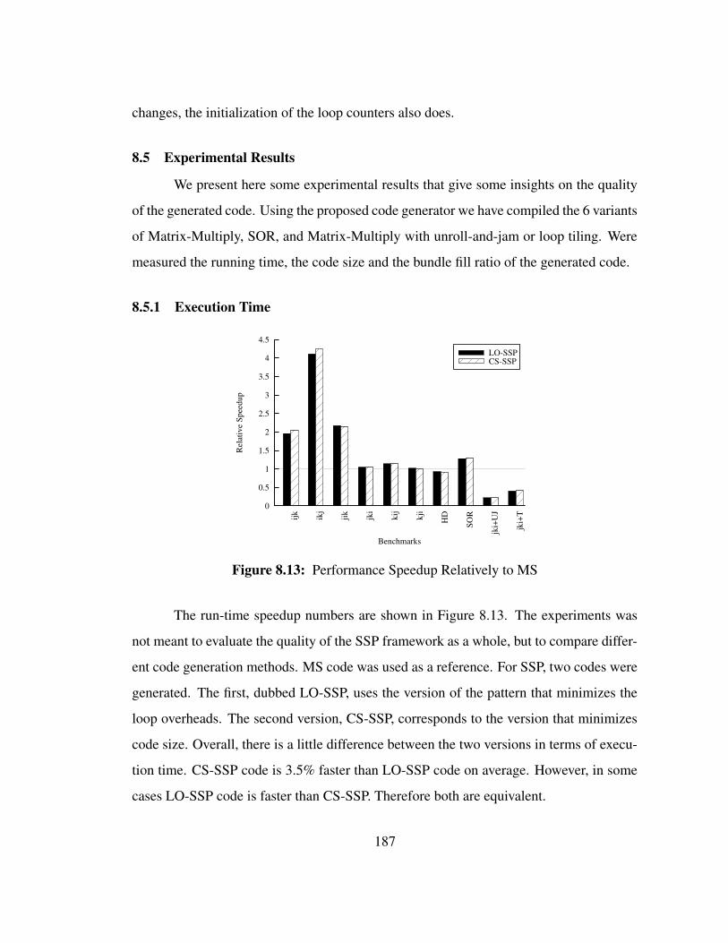
changes, the initialization of the loop counters also does.


We present here some experimental results that give some insights on the quality

of the generated code. Using the proposed code generator we have compiled the 6 variants

of Matrix-Multiply, SOR, and Matrix-Multiply with unroll-and-jam or loop tiling. Were

measured the running time, the code size and the bundle fill ratio of the generated code.


0

0.5

1

1.5

2

2.5

3

3.5

4

4.5

jki+

T

jki+

UJ

SOR

HDkji

kij

jki

jikikj

ijk

Rel

ativ

e Sp

eedu

p

Benchmarks

LO-SSPCS-SSP

Figure 8.13: Performance Speedup Relatively to MS

The run-time speedup numbers are shown in Figure 8.13. The experiments was

not meant to evaluate the quality of the SSP framework as a whole, but to compare differ-

ent code generation methods. MS code was used as a reference. For SSP, two codes were

generated. The first, dubbed LO-SSP, uses the version of the pattern that minimizes the

loop overheads. The second version, CS-SSP, corresponds to the version that minimizes

code size. Overall, there is a little difference between the two versions in terms of execu-

tion time. CS-SSP code is 3.5% faster than LO-SSP code on average. However, in some

cases LO-SSP code is faster than CS-SSP. Therefore both are equivalent.

187

8.5.2 Code Size

However, when it comes to code size, both code generation differ. The CS-SSP

is on average 1.67 times smaller than the LO-SSP code. Therefore limiting code size

explosion can efficiently be done at no cost in terms of run-time performance.

0

2

4

6

8

10

jki+

T

jki+

UJ

SOR

HDkji

kij

jki

jikikj

ijk

Rel

ativ

e C

ode

Size

Incr

ease

Benchmarks

LO-SSPCS-SSP

Figure 8.14: Code Size Increase Relatively to MS

On the other hand, when compared to MS, the code size is much higher (3.5 times

larger on average for CS-SSP). Several reasons explained those numbers. First, because

more than one loop level is considered, the SSP kernel is larger than the MS kernel.

Second, the lack of multiple levels of register rotation, forced us to duplicate code, which

represents 60% of the code or more. With proper hardware support, that duplication

would have been unnecessary.

Moreover the code size results must be considered with caution. Despite the no-

ticeable code size increase, the entire code of the schedule fits into the L1 instruction

cache of the processor. Run-time performance results in this chapter and in Chapter 3

have shown that SSP is still more efficient than MS to schedule loop nests. As long as no

performance degradation is noticed, the code size increase is not an issue.

188

8.5.3 Bundle Density

Finally we compare the bundle density for our three methods. On Itanium, a bun-

dle is contains one to three instructions that can be run in parallel. Measuring the average

number of operations within a bundle is an indirect way of measuring the instruction-level

parallelism exploited in the code. A higher values means a higher instruction-level par-

allelism degree. Overall CS-SSP code performs the best. On average a bundle contains

1.93, 1.93, and 2.11 instructions for MS, LO-SSP and CS-SSP respectively. Therefore

CS-SSP makes a better use of the available processor resources.

1

1.5

2

2.5

3

jki+

T

jki+

UJ

SOR

HDkji

kij

jki

jikikj

ijk

Bun

dle

Den

sity

(min

=1, m

ax=3

)

Benchmarks

MSLO-SSPCS-SSP

Figure 8.15: Bundle Density

Overall the code-size conscious code generation method drastically reduces the

code size and produces denser code while maintaining the same level of run-time perfor-

mance as the code generation that minimizes loop control overheads. CS-SSP is therefore

the method of choice to generate SSP code. The code size increase, although noticeable,

does not impair the schedule and the entire loop nest still fits in the L1 instruction cache.

8.6 Related Work

Code generation schemes for modulo scheduling of single loops are discussed

for VLIW architectures with and without hardware support in [RST92]. The considered

189

hardware support include rotating registers, predicated execution, and iteration control

registers [DT93]. The code generation approach for modulo scheduling in the Cydra-5

compiler has been discussed in [DT93]. Register allocation for software pipelined loops

has been considered in [RLTS92]. A number of alternative solutions have been presented

for machines with and without hardware support for software pipelining. Code size re-

duction for software pipelined loops has been discussed in [LF02, GSS+01]. All these

works consider software pipelining only for the innermost loop.

In contract, the solution presented in this chapter targets code generation issues for

the SSP method, which deals with multi-dimensional loop nests. Specific issues solved

include lack of multiple rotating register files, multiple patterns, loop overheads associ-

ated with the multiple loop levels, code size reduction, loop counter initialization.

8.7 Conclusion

This chapter presented a code generation scheme taking as an input a register-

allocated kernel that assumed multiple levels of register rotation. The proposed tech-

niques makes use of available hardware support such as predication, register rotation and

dedicated loop counters and make up for it through code duplication and register index

offsetting when that support is not available. Through the execution of repeating patterns

(OLP, DFP, ILP), the code remains compact and still fits in the L1 of the target architec-

ture.

Two methods were proposed. The first minimizes loop control overheads whereas

the second minimizes code size. Experimental results have shown that the latter is to

be preferred as it generates smaller and denser code while preserving the same level of

performance as the first method. Both methods tackle all the issues mentioned such as

loop counter initialization, unfriendly number of iterations, lifetimes interferences and the

innermost level separation constraint.

190

Chapter 9

MULTI-THREADED SSP

9.1 Introduction

The previous chapters described the different steps of the SSP framework up to

the code generation method for VLIW architectures with dedicated hardware loop sup-

port. In this chapter, we present how to software pipeline loop nests on multi-threaded

cellular architectures using Multi-Threaded Single-dimension Software-Pipelining (MT-

SSP). Starting from the ideal schedule, the multi-threaded final schedule is generated.

It is deadlock-free and fully synchronized. The proposed solution makes use of all the

thread units available in the cellular architecture without any modification to the source

code. The code generation algorithms are also presented. They take for input the same

SSP kernel than the code generation algorithms used for uniprocessor architectures in

Chapter 8.

The algorithms were implemented in the Open64 compiler retargeted to the IBM

64-bit Cyclops architecture and the multi-threaded final schedules run on the Cyclops

development team simulator. Experimental results show that the multi-threaded scales up

well when the number of thread units increases and that the number of stall cycles from

synchronization instructions is extremely low. Moreover, the average register pressure is

reasonable.

The chapter is organized as follows. The next section presents the Multi-Threaded

SSP theory along with the corresponding schedule function. Section 9.4 proposes an im-

plementation mechanism for the IBM 64-bit Cyclops architecture with an efficient syn-

chronization solution. Experimental results and related work are presented in Section 9.5

191

and Section 9.6, respectively. Concluding remarks are given in the last section.



In this chapter, we apply the Single-dimension Software Pipelining technique to

multi-threaded cellular architectures. We assume that the SSP ideal schedule has already

been computed and that registers have been allocated to the loop variants. A multi-

threaded version of the final schedule must now be computed. Therefore, the problem

we address here can be formulated as follows. Given a register-allocated SSP kernel,

generate a multi-threaded final schedule for multi-threaded cellular architectures.

Naturally, the multi-threaded final schedule will differ from the uniprocessor final

schedule presented in Chapter 3 and must first be defined. Section 9.3 presents the final

schedule for cellular architectures and the associated schedule function.

Despite the differences in the final schedule, the previous SSP steps, loop selec-

tion, kernel generation and register allocation, do not require any modification. Some

changes will be applied to the operations in the kernel, but the methods presented so far

are unchanged.

9.2.2 Issues

Multiple challenges must be faced to produce a multi-threaded final schedule.

First, the dependence and resource constraints must be respected. Similarly to the unipro-

cessor case, an operation cannot be scheduled before all the operations on which it de-

pends are committed. However, with multi-threaded architectures, extra attention must be

paid to memory operations. Memory dependences may exist between independent thread

units and synchronization is required to guarantee a sequential order between the memory

accesses to the same memory location.

The second challenge is the synchronization mechanism to be used. How to make

sure that a thread unit does not run ahead of the others? How to implement a light-weight

192

synchronization scheme? How to parameterize the synchronization mechanism so that the

execution time of the multi-threaded final schedule is minimized? If the synchronization

occurs too often, no useful work is done. If synchronization occurs too rarely, thread units

are idle waiting and no work is done.

The third issues concerns the workload distribution. Multi-threaded cellular archi-

tectures offer a large number of thread units. Dispatching tasks to thread units is costly.

Moreover, the distribution must be fair to keep all thread units as busy as possible in order

to minimize the overall execution time of the multi-threaded final schedule.

Fourth, cross-iteration dependences between outermost iterations scheduled on

separate thread units require thread units to communicate with each other. If the de-

pendence is a memory dependence, then synchronization must be used to guarantee that

memory locations contain the expected values. If the dependence is a register depen-

dence, extra code must be added and scheduled to communicate the register values from

one thread unit to the next. A register dependence occurs in the ideal schedule when an

operation in an outermost iteration accesses a value wrote into a register by another out-

ermost iteration. As long as the two outermost iterations are executed on the same thread

unit, the register is available to both. If the two iterations are scheduled on different thread

units, then the register of the first thread unit cannot be read the second thread unit.

Finally, as for every applications requiring synchronization, the multi-threaded

final schedule must be guaranteed deadlock-free.

9.3 Multi-Threaded SSP Theory

9.3.1 Multi-Threaded Final Schedule

The multi-threaded schedule is computed from the ideal schedule presented in

Section 3.2. In the ideal schedule, there may be some resource conflicts between out-

ermost iterations. To cope with the issue, the uniprocessor SSP schedule introduces a

delay every Sn outermost iterations. In the multi-threaded schedule, every group of Sn

iterations is instead executed on a separate thread unit. Sn, the number of stages of the

193

smallest subkernel, is the maximum number of outermost iterations that can be grouped

in the same iteration group without any resource conflict. With Sn+1 and above iterations,

two instances of the same innermost stage would be executed in parallel. The scheduling

constraints of the kernel does not guarantee that there will not be any resource conflict in

that scenario.

All the thread units end up executing the same code in a Single-Program Multiple-

Data (SPMD) fashion, simplifying the workload distribution and allowing thread units to

share the instruction cache.

op1

op2op3

op4op2op3

op4

op4

op2op3

op1

op2op3

op4op2op3

op4

op4

op2op3

op1

op2op3

op4op2op3

op4

op4

op2op3

op1

op2op3

op4op2op3

op4

op4

op2op3

0 1 2 3 i1

resource conflictsT=2

cycles

(a) Ideal Schedule

op1

op2op3

op4op2op3

op4

op4

op2op3

op1

op2op3

op4op2op3

op4

op4

op2op3

op1

op2op3

op4op2op3

op4

op4

op2op3

op1

op2op3

op4op2op3

op4

op4

op2op3

TU 0 TU 1

delay >= Tsynchronization

0 1 2 3 i1

iteration group (Sn=2)

extra waitinstruction

signalinstruction

instructionwait

extra signalinstruction

waiting

(b) Final Multi-Threaded Schedule

Figure 9.1: Multi-Threaded SSP Schedule Example

194

Naturally, the thread units require to be synchronized. Synchronization instruc-

tions are added to ensure that a thread unit does run ahead of its predecessor. In this

section, we assume the ideal case where those synchronization instructions can be ex-

ecuted at no cost. We also assume that the synchronization is non-blocking from the

sender’s point of view. The corresponding final schedule is then shown in Figure 9.1.

Although the figure suggests that synchronization signals are sent at regular interval, it

is not the case. Earlier wait instructions and other run-time variables prevent any regular

synchronization pattern to appear. The reader will notice that the first thread unit does not

have to wait for any synchronization signal to run. The position of the synchronization

points will be determined by code emission considerations as explained in Section 9.4.

In addition of the synchronization points mentioned above, a synchronization de-

lay must be introduced to guarantee the correctness of the final multi-threaded schedule.

Indeed, in the ideal schedule, a load instruction may access a value in memory that had

been stored in the same instance of the kernel. On a uniprocessor, such a memory depen-

dence would have been handled by the kernel generator. In the multi-threaded schedule,

the store instruction might appear in one iteration group and the load instruction in the

next. The memory would only be guaranteed to contain the correct value after the next

synchronization. Therefore, each iteration group must be delayed until the next synchro-

nization to ensure that the memory contains all the correct values. The duration of that

delay depends on the computed kernel. It is greater or equal to the initiation interval of

the kernel, T . Because an extra wait instruction is inserted before executing the itera-

tion group on the receiving thread unit, an extra signal instruction must be added after

the execution of the iteration group of the send thread unit so that the number of signal

instructions is equal to the number of wait instructions.

An example to explain the synchronization delay is shown in Figure 9.2. Let us

assume that op4 is a store instruction to a memory location which will be accessed by op3

two outermost iterations later. There is a memory dependence from op4 to op3. When

195

op2op3op4

op2

op1

op1

op2op3

load

store

sync

dependence

(a) No Stall

op1

op1

op2op3op3op4

op2

op2

at the same timeload and store executed

stall

sync

(b) A Memory Contention Occurs

Figure 9.2: Without Synchronization Delay Example

generating the kernel, the dependence was taken into account. If both iteration groups

were executed on the same processor, there would be no issue. Since the two iteration

groups are executed on separate thread units, the synchronization delay is required. If,

for instance, op2 is delayed because of memory access or floating-point unit contention in

the first iteration group and stalls the execution of the first thread unit, the second thread

unit will not be affected and continue running until op3 is executed and fetches the wrong

value from memory. If an extra wait instruction is added before executing the second

iteration group, a synchronization signal will be sent after op2 is executed, and op3 will

read the correct value from memory, as shown in Figure 9.3.

The reader would have noticed that synchronization signals are sent only from one

thread unit to its direct successor. Indeed, as explained in Section 3.2.2, there cannot be

any dependence from one outermost iteration to one of its predecessor. Those depen-

dences would require thread units to also synchronize their predecessors. Dependences

can only exist from one outermost iteration to either itself or one of the next outermost

196

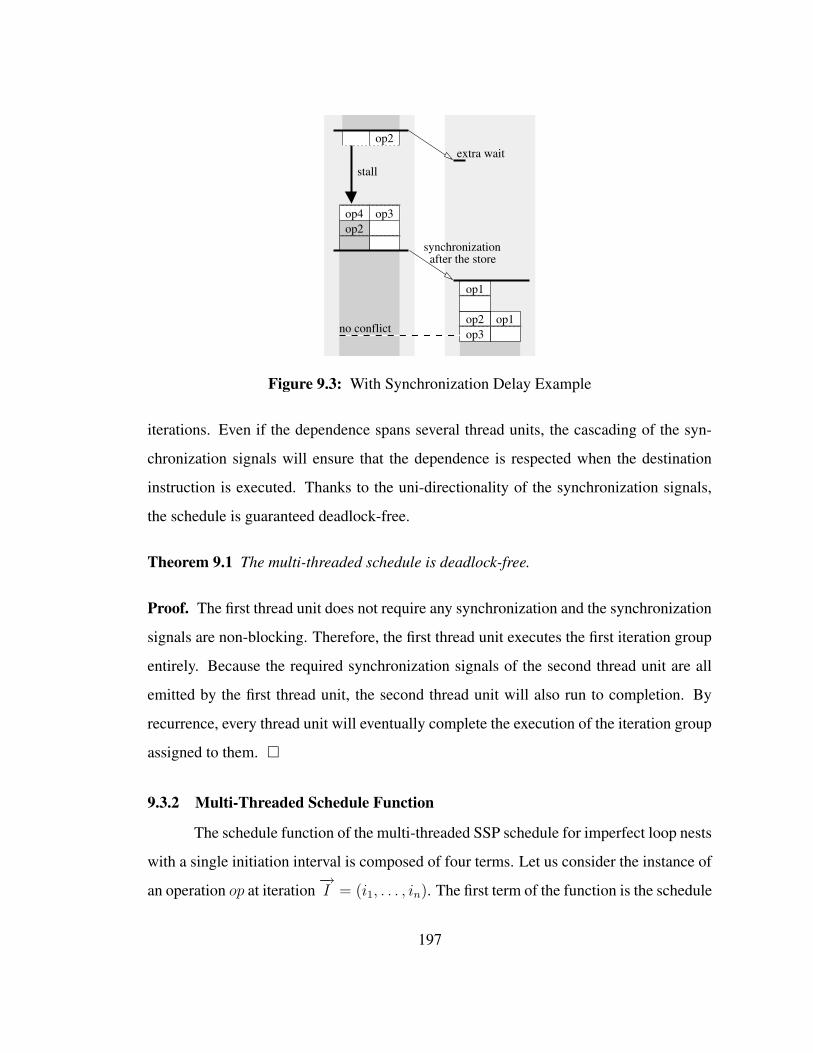
op3op4op2

op1

op1

op2op3

op2extra wait

no conflict

after the storesynchronization

stall

Figure 9.3: With Synchronization Delay Example

iterations. Even if the dependence spans several thread units, the cascading of the syn-

chronization signals will ensure that the dependence is respected when the destination

instruction is executed. Thanks to the uni-directionality of the synchronization signals,

the schedule is guaranteed deadlock-free.

Theorem 9.1 The multi-threaded schedule is deadlock-free.

Proof. The first thread unit does not require any synchronization and the synchronization

signals are non-blocking. Therefore, the first thread unit executes the first iteration group

entirely. Because the required synchronization signals of the second thread unit are all

emitted by the first thread unit, the second thread unit will also run to completion. By

recurrence, every thread unit will eventually complete the execution of the iteration group

assigned to them. �

9.3.2 Multi-Threaded Schedule Function

The schedule function of the multi-threaded SSP schedule for imperfect loop nests

with a single initiation interval is composed of four terms. Let us consider the instance of

an operation op at iteration−→I = (i1, . . . , in). The first term of the function is the schedule

197

cycle of the operation in the 1-D schedule, σ(op, 0). The second term is the start cycle of

the outermost iteration and is equal to:

i1 ∗ T (9.1)

The third term corresponds to the execution time of the inner iterations within the

current outermost iteration and is defined as:

k=n∑

k=2

ik ∗ timeLk (9.2)

where timeLk is the execution time of one iteration of the loop Lk within one

outermost iteration in the ideal schedule where operations have not been delayed yet:

timeLk =i=n∑

i=k

((Si − Si+1) ∗ T ∗

j=i∏

j=k+1

Nj

)

Sn+1 = 0

The last term is the synchronization delay explained in Section 9.3.1. Each thread

unit executes a single group of Sn outermost iterations. Each thread unit is delayed by a

minimum of T cycles from the previous thread unit. Therefore the synchronization delay

is expressed as:⌊i1Sn

⌋∗ T (9.3)

The schedule function of the multi-threaded SSP schedule for imperfect loop nests

with a single initiation interval can be written as shown in Figure 9.4. It assumes the ideal

case where synchronization takes 0 cycle and the synchronization delay only T cycles.

Theorem 9.2 Given an imperfect loop nest and an SSP kernel with a single initiation

interval for it, the schedule function proposed in Equation 9.4 respects both the depen-

dencies from the n-D DDG and the resource constraints.

198

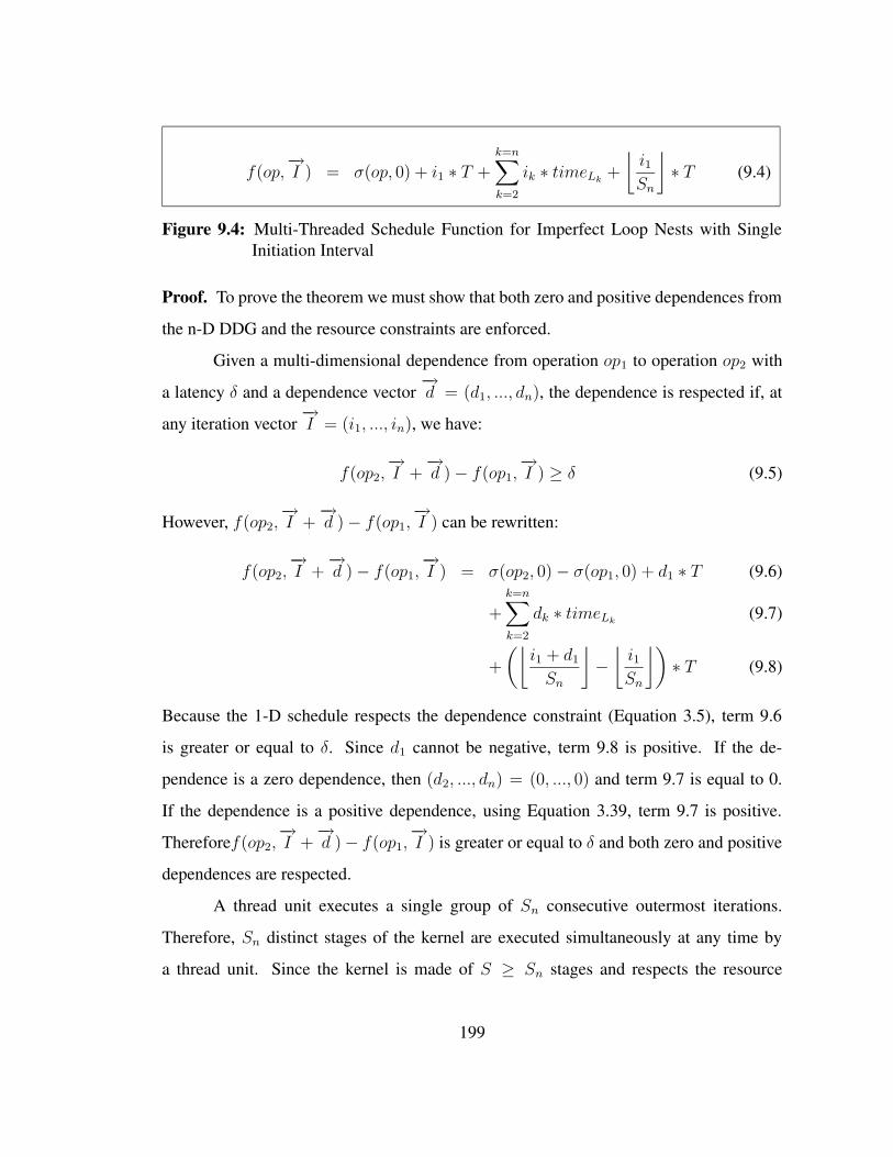
f(op,−→I ) = σ(op, 0) + i1 ∗ T +

k=n∑

k=2

ik ∗ timeLk +

⌊i1Sn

⌋∗ T (9.4)

Figure 9.4: Multi-Threaded Schedule Function for Imperfect Loop Nests with SingleInitiation Interval

Proof. To prove the theorem we must show that both zero and positive dependences from

the n-D DDG and the resource constraints are enforced.

Given a multi-dimensional dependence from operation op1 to operation op2 with

a latency δ and a dependence vector−→d = (d1, ..., dn), the dependence is respected if, at

any iteration vector−→I = (i1, ..., in), we have:

f(op2,−→I +−→d )− f(op1,

−→I ) ≥ δ (9.5)

However, f(op2,−→I +−→d )− f(op1,

−→I ) can be rewritten:

f(op2,−→I +−→d )− f(op1,

−→I ) = σ(op2, 0)− σ(op1, 0) + d1 ∗ T (9.6)

+k=n∑

k=2

dk ∗ timeLk (9.7)

+

(⌊i1 + d1

Sn

⌋−⌊i1Sn

⌋)∗ T (9.8)

Because the 1-D schedule respects the dependence constraint (Equation 3.5), term 9.6

is greater or equal to δ. Since d1 cannot be negative, term 9.8 is positive. If the de-

pendence is a zero dependence, then (d2, ..., dn) = (0, ..., 0) and term 9.7 is equal to 0.

If the dependence is a positive dependence, using Equation 3.39, term 9.7 is positive.

Thereforef(op2,−→I +−→d )− f(op1,

−→I ) is greater or equal to δ and both zero and positive

dependences are respected.

A thread unit executes a single group of Sn consecutive outermost iterations.

Therefore, Sn distinct stages of the kernel are executed simultaneously at any time by

a thread unit. Since the kernel is made of S ≥ Sn stages and respects the resource

199

constraints, no resource conflict can occur. Therefore the schedule function respects the

resource constraints. �

9.4 IBM 64-bit Cyclops Implementation

In this section, an efficient code generation method for multi-threaded final sched-

ules is presented. The target architecture is the IBM 64-bit Cyclops architecture, modified

to include rotating registers. The implementation make use of the available hardware re-

sources to correctly execute the schedules described in the previous section.

9.4.1 Overview

Iteration groups are executed on the thread units in a round-robin fashion. The

synchronization signals from the last thread unit are redirected from the non-existing next

thread unit to the first thread unit. The number of iteration groups does not have to be a

multiple of the number of thread units. Figure 9.5 shows an example where only 3 thread

units are available and 5 iteration groups are to be executed.

All the thread units but the first directly reach a wait instruction after their initial-

ization and will not start executing iteration groups until the first thread unit has started.

The thread unit to execute the last iteration group sends an extra synchronization comple-

tion signal to the first thread unit. When a thread unit has completed the execution of all

its iteration groups and has sent all the required signals, it goes to sleep. When the first

thread unit has received the completion signal from the last thread unit, it returns to the

main program.

9.4.2 Synchronization

Synchronization is implemented using a Lamport’s clock [Lam78]. Each thread

unit has two counters. The first counter, named synchronization counter, is used to count

the number of synchronization signals received so far. It is incremented by one each time

a signal is received. The second counter is the internal clock of the thread unit and called

200

init init

sleep

init

return

sleep

op1

op2op3

op4op2op3

op4

op4

op2op3

op1

op2op3

op4op2op3

op4

op4

op2op3

op1

op2op3

op4op2op3

op4

op4

op2op3

op1

op2op3

op4op2op3

op4

op4

op2op3

op1

op2op3

op4op2op3

op4

op4

op2op3

op1

op2op3

op4op2op3

op4

op4

op2op3

op1

op2op3

op4op2op3

op4

op4

op2op3

op1

op2op3

op4op2op3

op4

op4

op2op3

op1

op2op3

op4op2op3

op4

op4

op2op3

op1

op2op3

op4op2op3

op4

op4

op2op3

TU 0 TU 1 TU 2

extra waitinstruction

(1)

(1)

extra signalinstruction

completionwait

(2)

(2)

completionsignal

Figure 9.5: The Multi-Threaded Final Schedule on an IBM 64-bit Cyclops chip

201

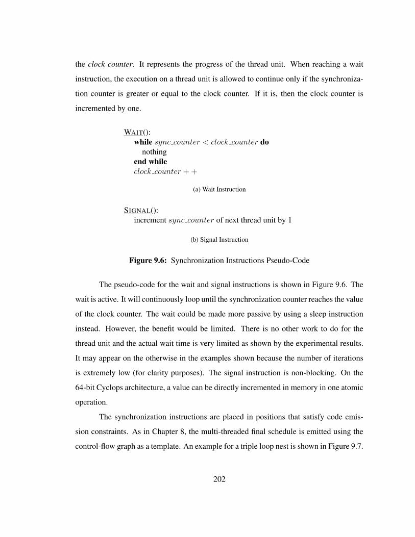
the clock counter. It represents the progress of the thread unit. When reaching a wait

instruction, the execution on a thread unit is allowed to continue only if the synchroniza-

tion counter is greater or equal to the clock counter. If it is, then the clock counter is

incremented by one.

WAIT():while sync counter < clock counter do

nothingend whileclock counter + +

(a) Wait Instruction

SIGNAL():increment sync counter of next thread unit by 1

(b) Signal Instruction

Figure 9.6: Synchronization Instructions Pseudo-Code

The pseudo-code for the wait and signal instructions is shown in Figure 9.6. The

wait is active. It will continuously loop until the synchronization counter reaches the value

of the clock counter. The wait could be made more passive by using a sleep instruction

instead. However, the benefit would be limited. There is no other work to do for the

thread unit and the actual wait time is very limited as shown by the experimental results.

It may appear on the otherwise in the examples shown because the number of iterations

is extremely low (for clarity purposes). The signal instruction is non-blocking. On the

64-bit Cyclops architecture, a value can be directly incremented in memory in one atomic

operation.

The synchronization instructions are placed in positions that satisfy code emis-

sion constraints. As in Chapter 8, the multi-threaded final schedule is emitted using the

control-flow graph as a template. An example for a triple loop nest is shown in Figure 9.7.

202

Innermost LoopPattern

Prolog

Draining/FillingPattern

Epilog

previous iteration group

next iteration group

N

N

−1n

−1i

Figure 9.7: Multi-Threaded SSP Schedule Control-Flow Graph for a Triple Loop Nest

When the schedule is partitioned into loop patterns named prolog, DFP, ILP, and epilog).

A wait instruction is added before each pattern and a signal instruction after.

In order to minimize the execution time of the wait instruction, the synchronization

counter is placed in the scratch-pad memory of the thread unit being signaled. The value

can then be quickly read by the receiving thread unit without using the crossbar network.

Although the signal instruction travels over the crossbar network, the signal instruction

is non-blocking. Therefore, the sending thread unit does not pay the cost of accessing

the scratch-pad memory of the receiving thread unit. The clock counter, which cannot be

accessed by the other thread units, is placed in a dedicated register of the thread unit for

fast access.

9.4.3 Innermost Loop Tiling

To reduce the number of synchronization stalls on a thread unit, the execution of

the Nn − 1 instances of the innermost loop pattern is tiled into tiles of G iterations. If G

203

ThreadUnit

Scratch−PadMemory

ThreadUnit

Scratch−PadMemory

Crossbar

Network

C S C S

remote non−blocking signal

local wait

synchronization counterclock counter

Figure 9.8: Location of the Synchronization Counters

is not a multiple of Nn − 1, the last tile only contains the remaining instances. Instead of

issuing a wait and signal instruction at the entrance and exit, respectively, of each instance

of the pattern, the synchronizations are issued every G instances as shown in Figure 9.9.

The technique allows for the parameterization of the synchronization tiling.

Let w designates the average execution time of the wait instruction. We can now

give an estimate of the total execution time of the schedule using the definition of the

multi-threaded schedule function for the IBM 64-bit Cyclops architecture. The last term

of Equation 9.4 is now better expressed by:(⌊

i1Sn

⌋− 1

)∗ (ln ∗ T +G ∗ Sn ∗ T ) (9.9)

ln∗T is the number of cycles executed by a thread before sending the first signal. G∗Sn∗Tis the number of cycles between the first signal and the second signal sent to the next

thread unit. The ILP is Sn ∗ T cycles long and a signal is sent after G executions of the

ILP.

Unlike the theoretical multi-threaded schedule function in Equation 9.4, we also

take into account the synchronization stalls of the entire schedule. That cost is carried to

204

op4op2op3

op2op3

op4

op4op2op3

op2op3

op4

op4op2op3

op2op3

op4

op4op2op3

op2op3

op4

ILP instance

(a) Before Tiling

op4op2op3

op2op3

op4

op4op2op3

op2op3

op4

op4op2op3

op2op3

op4

op4op2op3

op2op3

op4

tiled ILP

(b) After Tiling

Figure 9.9: Synchronization Tiling Example (G=2)

the last iteration group where it adds up to:⌊N1

Sn

⌋∗ 2 ∗ w + (syncsPerGroup− 2) ∗ w (9.10)

The first term corresponds to the 2 wait instructions used for the synchronization delay.

The delay accumulates over the iteration groups executed earlier. The second term corre-

sponds to the remaining wait instructions within one outermost iteration group.

Then, the total execution time of the schedule for the IBM 64-bit Cyclops archi-

tecture can be approximated by:

ftotal(G) = constant+

(⌊N1

Sn

⌋− 1

)∗ Sn ∗ T ∗G+ syncsPerGroup ∗ w

= constant+

(⌊N1

Sn

⌋− 1

)∗ Sn ∗ T ∗G

+w ∗ (Nn − 1) ∗(

1 +

j=n−1∏

j=2

(Nj − 1)

)∗ 1

G

205

Using the first derivative of the function, the best loop tiling factor for which the total

execution time is minimized, Gbest, can be computed and is equal to:

Gbest =

√√√√√w ∗ (Nn − 1) ∗

(1 +

∏j=n−1j=2 (Nj − 1)

)

T ∗ Sn ∗(⌊

N1

Sn

⌋− 1) (9.11)

The best empiric value for G is studied in Section 9.5.

9.4.4 Synchronization Bootstrapping

The first iteration group, executed on the first thread unit, does not receive any

synchronization signal during its execution. Therefore, the flow of execution should fall

through the wait instructions of that iteration group. Such feature is achieved by setting

the synchronization counter to the number of synchronization signals that an iteration

group needs to receive to run to completion, defined as syncsPerGroup. That number is

equal to the number of instances of each pattern to which we add the extra wait instruction

used for the synchronization delay (extra = 1). In one iteration group, the prolog is

executed only once (P = 1). So is the epilog (E = 1). The number of times DFPi is

executed, noted Di with i ∈ [2, n− 1], is given by:

Di = (Ni − 1) ∗Di−1 with D1 = P =

j=i∏

j=2

(Nj − 1)

The number of times the tiled ILP is executed, noted I , can be expressed as:

I =Nn − 1

G∗ (Dn−1 + P ) =

Nn − 1

G∗(

1 +

j=n−1∏

j=2

(Nj − 1)

)

206

Then we have:

syncsPerGroup

= extra+ P + I + E +i=n−1∑

i=2

Di

= 3 +Nn − 1

G∗(

1 +

j=n−1∏

j=2

(Nj − 1)

)+

i=n−1∑

i=2

j=i∏

j=2

(Nj − 1)

= 3 +Nn − 1

G+Nn − 1

G∗j=n−1∏

j=2

(Nj − 1) +i=n−1∑

i=2

j=i∏

j=2

(Nj − 1) (9.12)

IfNn−1 is not a multiple ofG, (Nn−1)/Gmust be replaced by b(Nn−1)/Gc+1

to account for the extra wait instructions. If the loop nest is a double loop nest, then the

last two terms of Equation 9.12 are equal to zero.

The synchronizations signals sent by the thread unit that executes the last outer-

most iteration group are received by the next thread unit, even if that thread unit is not

required to execute any other outermost iteration. Afterward the completion signal is sent

to the first thread unit.

9.4.5 Cross-Iteration Register Dependences

When distributing iteration groups over the thread units, an issue arises with the

cross-iteration register dependences. Those dependences are dependences between out-

ermost iterations involving values in registers and not spilled in memory. It is typical

an outermost loop counter for instance. On a uniprocessor, the problem does not exist

as there is a single register file. However, in the IBM 64-bit Cyclops architecture, each

thread unit has its own private register file which cannot be accessed by any other thread

unit. Values involved in a cross-iteration register dependence need to be copied from one

thread unit to the next.

A solution is to transform the register dependence into a memory dependence.

We issue memory spill instructions to copy the value from the register to a buffer in the

scratch-pad memory of the destination thread unit. The value is then restored using a

207

single memory load. The scratch-pad memory of the receiving thread unit was chosen

because memory spills are non-blocking and memory restores from the local scratch-pad

memory does not involve the crossbar network and can be executed in a matter of few

cycles. As the cross-iteration register dependences are known at compile-time, the buffer

and offset to its respective values are statically allocated.

TU i+1TU i

scratch−pad memory

...=R

restore

spill

R=R+1

...=R

restore

spill

R=R+1

R=R+1...=R

...=RR=R+1

buffer

localaccess

remoteaccess

cross−iteratonregister dependence

memory dependencecross−iteration

unnecessary memory

not emittedspills and restores are

register value accessedin next outermost iteration

known offset

Figure 9.10: Cross-Iteration Register Dependence Example

Memory spill instructions only need to be issued by the last outermost iteration

208

of an iteration group and memory restore instructions by the first. Within an instruction

group, the value is transferred from one outermost iteration to the next using registers as

usual. If the value is to be used by another outermost iteration than the next (meaning

that the distance of the cross-iteration register dependence is greater than 1), register

copies and memory spills/restores will bring that value to the recipient outermost iteration

naturally in a cascade fashion.

The mechanism is implemented by adding memory spill and restore instructions

at the ends of each cross-iteration dependence during the loop selection phase in the SSP

framework. The kernel generator then produces an SSP kernel which contains those extra

operations. While emitting the assembly code, the memory spill operations are removed

from every iteration but the last of an iteration group, and the memory restore operations

are removed from every iteration but the first of an iteration group. The removal of those

operations is accompanied by some register renaming to take the change into account.

Figure 9.10 shows an example of a cross-iteration register dependence. Register

R is used and then incremented by one in the first outermost iteration. The next outer-

most iteration uses the incremented value and increments again the value in the register.

Because the two outermost iterations are executed on the same thread unit, the register

is accessible to both iterations. However, the third iteration cannot access that register.

Instead, the value is spilled into a known location by the second iteration. The third iter-

ation retrieves the value from the buffer before using it. The spill and restore instructions

only appear in the first and last outermost iterations of an iteration group.

9.4.6 Code Generation Algorithms

The pseudo-code skeleton of the multi-threaded final schedule is shown in Fig-

ure 9.11. The details of the loop patterns are shown in Figure 9.12. The code is common

to all thread units and loaded to each thread unit. Then the first thread unit will initiate

the execution of the entire schedule when sending its first synchronization to the next

thread unit. The main loop iterates over the iteration groups that each thread unit must

209

[Initialization]

// Iterate over the iteration groupsi1 ← my thread idwhile i1 < N1 do

i1 ← i1 + num TUsclock counter ← clock counter + 1 // synchronization delay[Prolog]

for i2 = 0, N2 − 1 dofor i3 = 0, N3 − 1 do

. . .// Tiled ILPfor i = 1, (Nn − 1)/G do

wait()for g = 1, G do

[ILP]end forsignal()

end for. . .if i3 < N3 − 1 then

[DFP3]end if

end forif i2 < N2 − 1 then

[DFP2]end if

end for

rotate registers()[Epilog]signal() // extra signal for synchronization delay

end while

[Conclusion]

Figure 9.11: Multi-Threaded Code Skeleton

210

execute. Before executing one iteration group, the clock counter is incremented to force

the synchronization delay. An extra signal is added after executing each iteration group.

[Prolog] =wait()for i = f1, ln − 1 do

Emit Stages(f1, l1, Sn, 1, 0, i− f1 − (Sn − 1), ln − f1)if i < ln − 1 then

rotate registers()end if

end forsignal()

[ILP] =for i = 0, Sn− 1 do

Emit Stages(fn, ln, Sn, n,−i− 1, i, Sn)end for

[DFPlvl] =wait()for i = 0, llvl − flvl do

Emit Stages(flvl, llvl, Sn, lvl,−i− 1, fn − flvl + i, llvl − flvl + 1)end forsignal()

[Epilog] =wait()for i = ln, l1 + Sn− 1 do

Emit Stages(f1, l1, Sn −max(i− l1, 0), 1, 0, i− Sn + 1, l1 − ln + 1)rotate registers()

end forsignal()

Figure 9.12: Loop Patterns Expansion

Compared to the uniprocessor code for the Intel Itanium architecture presented in

Chapter 8, there is no outermost loop pattern anymore and the innermost loop pattern is

now tiled. Register rotation is still required in the prolog and epilog. The register rotation

emulation technique used for the other patterns is similar to the Itanium version and will

211

not be described here. The patterns are now surrounded by synchronization instructions: a

wait instruction before each pattern and a signal after. The synchronization instructions

for the innermost loop pattern are moved into the outer tiled loop.

EMIT STAGES(first stage, last stage, stage count, level, register offset,stage offset, total height)

for cycle = first cycle[level], f irst cycle[level] + T [level]− 1 dostage counter ← stage count

reg offset← register offsetstage← first stage+ stage offsetwhile stage ≤ last stage and stage counter > 0 do

if (operation is memory spill and stage counter 6= stage count)or (operation is memory restore and stage counter 6= 1) then

do not emit this operationend ifemit ops(level, stage, cycle, reg offset)stage counter ← stage counter − 1stage← stage+ 1

end while

reg offset← register offset+ total heightstage← first stagewhile stage counter > 0 do

if (operation is memory spill and stage counter 6= stage count)or (operation is memory restore and stage counter 6= 1) then

do not emit this operationend ifemit ops(level, stage, cycle, reg offset)stage counter ← stage counter − 1stage← stage+ 1

end whileend for

Figure 9.13: Stage Emission Algorithm

The stage emission routine, Emit Stages(), shown in Figure 9.13, also differs

from the Itanium version to take into account the features of the multi-threaded schedule

and the absence of predicate registers in the IBM 64-bit Cyclops architecture. The register

212

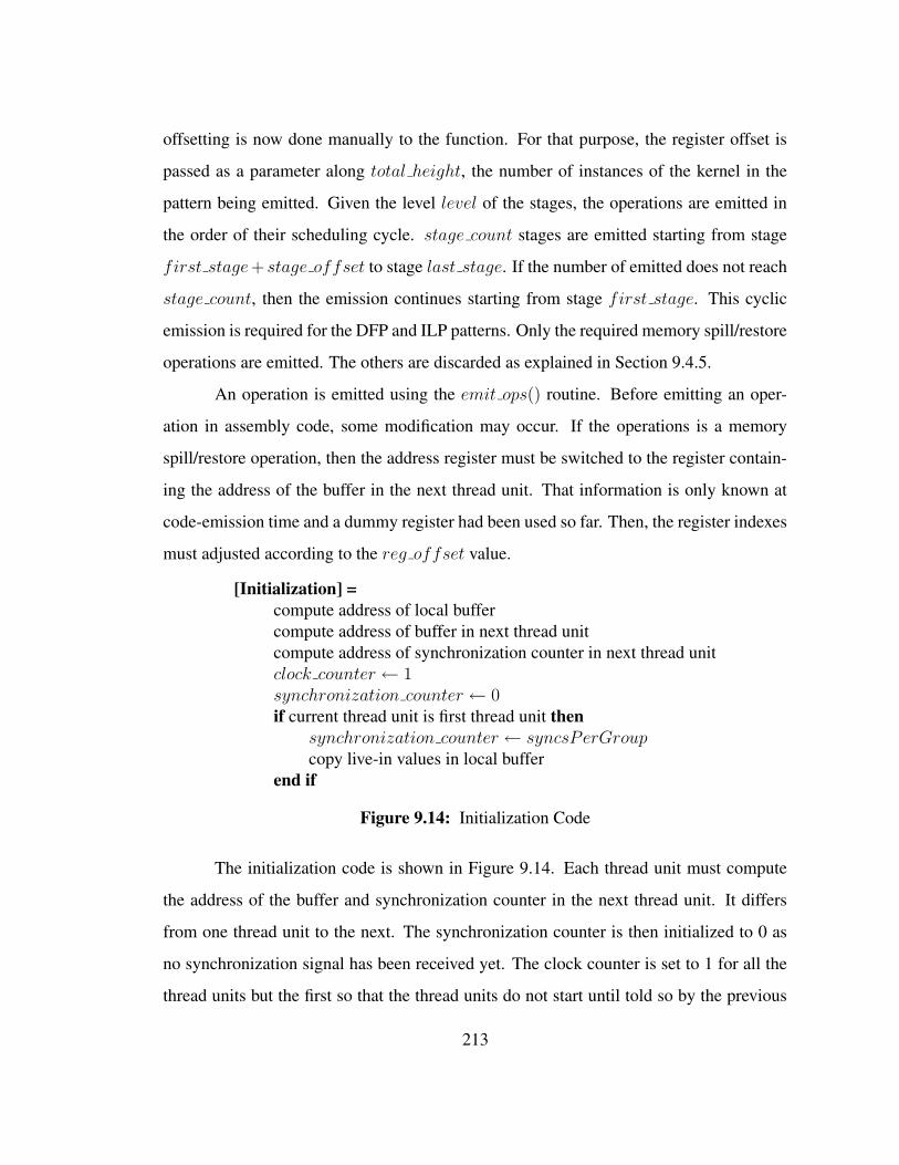
offsetting is now done manually to the function. For that purpose, the register offset is

passed as a parameter along total height, the number of instances of the kernel in the

pattern being emitted. Given the level level of the stages, the operations are emitted in

the order of their scheduling cycle. stage count stages are emitted starting from stage

first stage+ stage offset to stage last stage. If the number of emitted does not reach

stage count, then the emission continues starting from stage first stage. This cyclic

emission is required for the DFP and ILP patterns. Only the required memory spill/restore

operations are emitted. The others are discarded as explained in Section 9.4.5.

An operation is emitted using the emit ops() routine. Before emitting an oper-

ation in assembly code, some modification may occur. If the operations is a memory

spill/restore operation, then the address register must be switched to the register contain-

ing the address of the buffer in the next thread unit. That information is only known at

code-emission time and a dummy register had been used so far. Then, the register indexes

must adjusted according to the reg offset value.

[Initialization] =compute address of local buffercompute address of buffer in next thread unitcompute address of synchronization counter in next thread unitclock counter ← 1synchronization counter ← 0if current thread unit is first thread unit then

synchronization counter ← syncsPerGroupcopy live-in values in local buffer

end if

Figure 9.14: Initialization Code

The initialization code is shown in Figure 9.14. Each thread unit must compute

the address of the buffer and synchronization counter in the next thread unit. It differs

from one thread unit to the next. The synchronization counter is then initialized to 0 as

no synchronization signal has been received yet. The clock counter is set to 1 for all the

thread units but the first so that the thread units do not start until told so by the previous

213

thread unit. The clock counter of the first thread unit is initialized with the number of

synchronizations per iteration group to be able to execute the first iteration group without

requiring any synchronization signal. The live-in values are copied in the local buffer of

the first thread unit to bootstrap the execution.

[Conclusion] =if current thread unit executes last iteration group then

signal the first thread unitend ifif current thread unit is first thread unit then

wait()else

sleep()end if

Figure 9.15: Conclusion Code

The conclusion code is shown in Figure 9.15. The thread unit to execute the last

iteration group signals the first thread unit that the schedule is completed. All the thread

units, but the first, then go to sleep (or terminate). The first thread units waits for the

completion signal to arrive and returns.

In order to reduce the execution time of the schedule, the loop control instructions,

such as iteration index increment and trip count comparison, have been added to the

operations of the loop nest and therefore scheduled in the kernel. As such, the register

offset has been applied to the loop counter registers. The only instruction that has not been

scheduled in the kernel is the branch instruction. Therefore, the register offset must also

be applied to the branch instruction. The loop control register used should correspond to

the one last defined in the last outermost iteration in an iteration group.

9.4.7 Correctness

We present here two theorems that goes towards proving that the IBM 64-bit Cy-

clops multi-threaded schedule is correct.

214

Theorem 9.3 The synchronization signal guarantees that the memory accesses preceding

it have been committed.

Proof. The accesses to the crossbar network are managed in first-in first-out order at

the sending network port. A memory access will not travel across the network until the

receiving side can handle the memory access atomically. Therefore the memory accesses

issued over the network are guaranteed to be executed in sequential order from the point

of the view of the sending thread unit. In consequence, this property also guarantees that

when a signal instruction is issued, the preceding memory accesses have already been

committed. �

Theorem 9.4 The IBM 64-bit Cyclops multi-threaded final schedule is deadlock-free.

Proof. The signal instruction is non-blocking. We already proved in Theorem 9.1 that,

giving that condition, the multi-threaded final schedule was deadlock-free. The IBM 64-

bit Cyclops implementation adds the round-robin execution of the iteration groups and the

use of buffers. Buffer accesses are normal memory operations and do not change anything

to the correctness of the schedule. And the recurrence proof used in Theorem 9.1 can still

be applied despite the round-robin execution. �


The multi-threaded SSP method was implemented in the Open64 compiler retar-

geted for the IBM 64-bit Cyclops architecture. The earlier steps up to the register alloca-

tion were also added unmodified to the compiler. Fourteen loop nests from the Livermore

Suite, SPEC2000 and NAS were compiled and evaluated using the simulator used by the

development team of the IBM 64-bit Cyclops architecture. Loop tiling factor of 1, 2, 4, 8,

16, 32, 64, and 128 were tested on the processor with 99 thread units. The execution time

absolute speedup was measured with 1, 3, 7, 15, 31, 63, and 99 thread units with the best

loop tiling factor measured. The issue width of a thread unit was assumed to be equal to

215

2 and the register file was assumed to be rotating. The problem size of each benchmark

was chosen as large as possible under the constraint that the simulator could compute the

output in 60 minutes for a total simulation time of 196 hours.

9.5.1 Execution Time Speedup

The scalability results for a representative set of benchmarks are shown in Fig-

ure 9.16. The best loop tiling factor for each benchmark was chosen. As the number of

thread units increases, the total execution time of the benchmarks dramatically reduces.

The ikj variant of matrix-multiply shows the best result with an absolute speedup of 81

for 100 thread units. The worst speedup, 42 for 100 thread units, was encountered when

evaluating benchmark livermore18.3.

0

20

40

60

80

100

100 64 32 16 8 4 2

Exe

cutio

n T

ime

Abs

olut

e Sp

eedu

p

Number of Thread Units

linear

speed

upmm-ikjsorg3hydroblaslivermore 18.3

Figure 9.16: Execution Time Absolute Speedup

Ideally, the execution time absolute speedup is linear. The difference is explained

by two facts. First, cross-iteration dependences prevent the outermost iteration group from

being executed in parallel and achieving a linear speedup. The second explanation is the

fixed cost of initializing the schedule. With 100 thread units, the cascaded initialization

of all the thread units is costly: thread unit i will not start before receiving two signals

from thread unit i − 1. Given a fixed number of outermost iterations, the more thread

units are used, the higher the initialization cost becomes. If the number of outermost

216

iterations is too small, the initialization becomes the dominant factor in the total execution

time. This explains why the difference between speedup curves and the linear speedup

curve increases as the number of thread units increases. When the number of outermost

iterations increases, so does the execution time speedup. For instance, when the number

of outermost iterations of the worst performing benchmark, livermore18.3, is multiplied

by a factor of only 4, the speedup for 99 thread units jumps from 42 to 67 1.

9.5.2 Loop Tiling Factor

The best loop tiling factor was searched for each of the benchmarks running on

the IBM 64-bit Cyclops processor with 99 thread units. A representative set of results are

shown in Figure 9.17. Overall, the benchmarks can be partitioned into 2 groups. In the

first group, loop tiling helps reducing the execution time of the benchmarks. For instance,

the ijk variant of matrix-multiply shows a speedup of 1.29 with a tile factor of 32 or

64. The second group, which includes blas, hydro and livermore18.3 in the graph, only

shows deteriorating speedup as the tiling factor increases.

0

0.2

0.4

0.6

0.8

1

1.2

1.4

1.6

128 64 32 16 8 4 2

Exe

cutio

n T

ime

Spee

dup

Loop Tiling Factor (G)

mm-ijkmm-kijg3blashydrolivermore 23

Figure 9.17: Loop Tiling Factor

1 Although increasing the problem size for all the benchmarks would improve thespeedup results, it was not attempted because of the time required to run the bench-marks on the IBM 64-bit Cyclops simulator.

217

The experimental results are in line with theoretical best value for G computed

in Equation 9.11. The best value for G for the benchmarks in the second group happens

to be 1 because the number of iterations of the inner loops is not large enough. Using

the measured average execution time of the wait instruction (14 cycles), the difference in

total execution time using the empirical best value for G and the theoretical best G value

(Gbest) was measured. The maximum recorded difference was 1.7% with an average of

0.3%. Gbest is therefore a very accurate approximation of the best value to be chosen for

G.

9.5.3 Synchronization Stalls

The stall cycles were measured for all the benchmarks and using 100 thread units

with the best loop tiling factor. The average execution time of the wait is 14 cycles

(synchronization delays excluded). It is exactly the time it takes to execute the instruction

when the data are already in the buffer. Therefore, the wait instruction never blocks.

The value could be further reduced by implementing the wait instruction as an atomic

instruction in the instruction set architecture.

However, such a dedicated instruction would have almost no impact on the total

execution time of the schedules. On average, the number of cycles to execute the wait

instructions represents only 0.2% of the total execution time with a maximum of 0.7%.

The cost of the wait instruction is therefore negligible.


Finally, the register pressure was measured for each of the benchmark. The

average register pressure was measured at 55.1 registers with a maximum of 96 for

livermore8. That pressure is reasonable and much lower than for the Intel Itanium ar-

chitecture, considering that IBM 64-bit Cyclops registers are used both for floating-point

and integer values. Such difference is explained by the reduced issue width of the IBM

64-bit Cyclops processor. A limited issue width increases the initiation interval of the

218

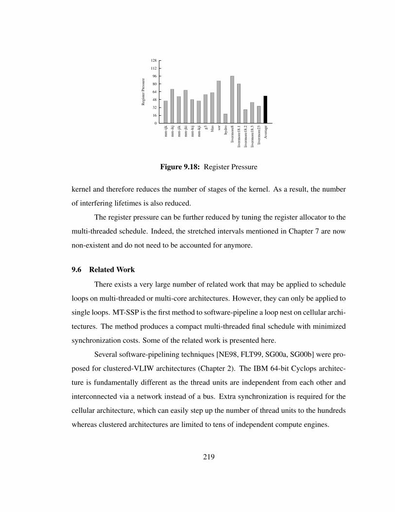
0

16

32

48

64

80

96

112

128

Ave

rage

liver

mor

e23

liver

mor

e18.

3

liver

mor

e18.

2

liver

mor

e18.

1

liver

mor

e8

hydr

o

sor

blasg3

mm

-kji

mm

-kij

mm

-jki

mm

-jik

mm

-ikj

mm

-ijk

Reg

iste

r Pre

ssur

e

Figure 9.18: Register Pressure

kernel and therefore reduces the number of stages of the kernel. As a result, the number

of interfering lifetimes is also reduced.

The register pressure can be further reduced by tuning the register allocator to the

multi-threaded schedule. Indeed, the stretched intervals mentioned in Chapter 7 are now

non-existent and do not need to be accounted for anymore.

9.6 Related Work

There exists a very large number of related work that may be applied to schedule

loops on multi-threaded or multi-core architectures. However, they can only be applied to

single loops. MT-SSP is the first method to software-pipeline a loop nest on cellular archi-

tectures. The method produces a compact multi-threaded final schedule with minimized

synchronization costs. Some of the related work is presented here.

Several software-pipelining techniques [NE98, FLT99, SG00a, SG00b] were pro-

posed for clustered-VLIW architectures (Chapter 2). The IBM 64-bit Cyclops architec-

ture is fundamentally different as the thread units are independent from each other and

interconnected via a network instead of a bus. Extra synchronization is required for the

cellular architecture, which can easily step up the number of thread units to the hundreds

whereas clustered architectures are limited to tens of independent compute engines.

219

Decoupled Software-Pipelining [ORSA05] schedules a single loop over multiple

thread units. Instead of distributing the iterations over the thread units, the same thread

unit always executes the same group of operations. Thus, if an iteration can be partitioned

into groups, the first thread unit executes the first group of every iteration, the second

thread unit the second group and so on. However, if the number of thread units reaches

the hundreds, the thread units cannot be kept busy.

Other multi-threading techniques include speculative multi-threading with run-

time analysis, also called run-time parallelization of DOACROSS loops [Che94, TY96,

THA+99]. Threads are speculatively issued and killed as information about the execu-

tion of loops is known. Although those methods allow for a wider range of loops to be

scheduled, especially with pointer-chasing structures, the thread control overheads are

very high compared to MT-SSP.

Some work [dCZG06] was also done to efficiently port OpenMP to the IBM 64-bit

Cyclops architecture. However, OpenMP is high-level language requiring extra interven-

tion from the programmer and suffering from generic constructs overheads. MT-SSP is

directly applied at the instruction level and exclusively target loop nests.

9.7 Conclusion

In this chapter we presented a solution to software pipeline loop nests on multi-

threaded cellular architectures based on SSP. The method is named Multi-Threaded

Single-dimension Software-Pipelining (MT-SSP). Given the SSP kernel, a fully synchro-

nized multi-threaded final schedule is generated to efficiently execute the loop nest with-

out any modification to the source code. The schedule is proven deadlock-free and respect

all the dependence and resource constraints.

Code generation algorithms were presented for the IBM 64-bit Cyclops architec-

ture. Synchronization is done through the use of a Lamport’s clock on each thread unit.

The signal instruction is non-blocking to allow for faster execution. The synchroniza-

tion counter is placed in the local scratch-pad memory of the receiving thread unit to

220

limit network accesses and drastically reduce the execution time of the wait instruction.

Cross-iteration register dependences between thread units were handled through the use

of memory spill and restore operations to and from a buffer also in the scratch-pad mem-

ory of the receiving thread unit. Those operations are scheduled in the kernel.

Experimental results showed that multi-threaded SSP schedules scales up well

when the number of thread units increases. The implementation uses a very light-weight

synchronization method with only standard instructions of the IBM 64-bit Cyclops archi-

tecture. The loop tiling factor was shown to be correctly approximated using the definition

of Gbest. Finally, the register pressure appeared to be reasonable without taking any extra

steps to reduce it.

221

Chapter 10

CONCLUSION

10.1 Summary

This dissertation has introduced SSP, Single-dimension Software-Pipelining, as a

valid approach to schedule loop nests on both uniprocessors and cellular architectures. In

the search for more computational power, computer architects have reached a technology

wall. Increasing clock speed, on-chip cache, pipeline depth and the number of functional

units on uniprocessors does not suffice anymore. When power consumption and cooling

systems are added to the financial equation, the return on investments has clearly passed

the point of diminishing return.

This fact leads to a new generation of processor architectures based on a large

number of parallel threads running on simple but power-efficient thread units: cellular

architectures. The thread units are interconnected via a network and share memory dis-

tributed in banks also connected to the network. By distributing the computation power

over the entire chip and by reducing the hardware complexity, the power consumption

and cooling issues disappeared. Also, because a defect thread unit or memory bank does

not prevent the chip from running properly, defect chips can still be used. The production

of a cellular processor then shows a high yield and results in lower manufacturing costs,

alleviating the price barrier to enter the processor market.

However, the programmability issue still remained to be solved. How to program

applications that will rip the benefits of so much parallelism? How to synchronize the

threads executing on all the thread units? How to communicate data from one thread to

222

another in a timely fashion? This dissertation presented SSP, a method aimed at provid-

ing a solution to all those questions for loop nests, a program structure present in many

applications and which can represent up to 90% of the execution time in the scientific

domain.

SSP is a whole compilation framework which takes loop nests as an input at the

programming language level and produces the schedule in assembly code to execute the

loop nest on either a VLIW architecture or a cellular architecture. The different steps of

the methods were first implemented for a VLIW architecture with convenient loop dedi-

cated hardware support such as register rotation, predication and dedicated loop counters,

before being ported to cellular architectures. The entire framework for both VLIW and

cellular architectures are presented in this dissertation.

We first presented the theoretical framework behind SSP. Given a loop nest and

its multi-dimensional data dependence graph, the most profitable loop level is selected.

Profitability is based on criteria set by the user and is heuristic-based. The user might want

to reduce execution time, limit network traffic or reduce power consumption. Once a level

has been selected, the multi-dimensional dependence graph is simplified into a single-

dimension data dependence graph which will be used to generate the schedule for the loop

nest. The schedule functions for both perfect and imperfect loop nests are introduced,

along with their properties and correctness proofs. SSP is proved to subsume modulo

scheduling (MS) as a special case when the loop nest is a single loop. Experimental results

show that SSP schedules are faster than MS schedules for a large set of benchmarks, even

after loop nest transformations and optimizations such as loop tiling are used.

The different steps to generate the final schedule are then introduced. First, some

loop selection heuristics are presented. Then the design principles of three scheduling

methods are presented. All methods produce a kernel which is used to build the final

schedule of the loop nest. The first method schedules operations one loop level at a time

223

starting from the innermost. The second method schedules all the operations simulta-

neously, expanding the search space and therefore increasing the possibility of finding a

better solution. Finally, the last method is an hybrid approach between the first two in

order to overcome the disadvantages of both other methods. Experiments showed that

the second approach is too slow while the first and third methods find reasonably good

solutions.

When the kernel is computed, a fast and accurate scheme was presented to evaluate

the register pressure in the final schedule of the loop nest before even allocating register

to the loop variants of the loop nest. The evaluation is used to decide to continue with

computed kernel. If the register pressure is deemed too high and the architecture does not

provide enough registers to accommodate the schedule needs, then another loop level is

chosen or another kernel with a lower register pressure is computed. Experimental results

showed that the integer register pressure increases with the depth of the loop nest whereas

the floating-point register pressure tends to remain constant. With 128 integer registers

and 64 floating-point registers, most of the loop nests can be scheduled with SSP.

Then, we presented a normalized representation of the complex lifetimes of an

SSP schedule. The design allows for a fine-grain representation of the holes with those

lifetimes to allow for their interleaving on the register space-time cylinder. A method

is proposed to exploit the representation and compute a register allocation solution that

minimizes register usage. Results prove the importance of minimizing register usage and

show that the computed solutions are close to optimality.

A code generation scheme was also presented for the Intel Itanium VLIW archi-

tecture. The solution takes advantage of the available hardware support. To limit code

size expansion, register rotation, predication and dedicated loop counters were used. To

cope with the lack of multiple rotating register files, modulo-variable expansion with code

duplication was used. Experimental results showed that, despite the code size increase,

the memory footprint of the final schedule still fits in the L1 instruction cache.

224

Finally, we presented a code generation scheme for the IBM 64-bit Cyclops cellu-

lar architecture. The SSP schedule was modified into an Multi-Threaded SSP (MT-SSP)

schedule to accommodate the presence of the many thread units and the synchroniza-

tion needs. The provided solutions generate a multi-threaded synchronized schedule for

the loop nests that fully utilizes the computational power of the machine. Experimental

results showed that the performance increases linearly with the number of thread units.

10.2 Future Work

While this dissertation proved that SSP is a viable loop nest scheduling solution

for both VLIW and cellular architectures, there are many directions for future research.

The first direction is to increase the set of loop nests to which SSP can be applied

to. Currently, a loop level cannot be selected if it contains a negative dependence. How-

ever, it is entirely possible to transform the loop nest via loop skewing or loop retiming

to make the negative dependence disappear. It would transform the rectangular iteration

space into a parallelogram iteration space which would require some loop peeling. Also,

loop nests could include loop siblings, i.e. two or more consecutive loops at the same

loop level. Several kernels would have to be created and adjusted to match. The register

allocator would have to be modified to take into account the multiple kernels. Finally,

conditional statements should be accepted by SSP. The Itanium architecture offers a way

to convey the value of predicate register used as a guarding predicate of a predicated

instruction. Thus conditional statements could be if-converted and loop nests software-

pipelined. If the hardware does not support predication, reverse if-conversion could also

be used [WBHS92, WMHR93].

Second, the register pressure remains an issue, especially if more complex loop

nests with loop siblings and conditional statements are to be considered. Since the reg-

ister allocator already generates almost optimal solutions, the attention should be set to

the other steps of the SSP framework. One can imagine a set of loop nest transformations

before SSP that would reduce the register pressure of a given level. The loop selection

225

step could also avoid levels that are guaranteed to have a register pressure that is too high.

The register pressure evaluation mechanism could be modified to become incremental

and merged to the scheduler to generate register pressure oriented kernels. Also, inserting

register spill and restore instructions to the schedule to limit the number of stretched life-

times would strongly reduce the register pressure of SSP schedules. Finally, in MT-SSP,

the register allocator could be adapted to take into account the lifetimes features of the

multi-threaded final schedules. Currently, the register allocator conservatively assumes

an uniprocessor final schedule.

Third, some cross-iteration register dependences could be eliminated from the

ideal schedule in order to decrease the amount of memory accesses on a multi-threaded

cellular chip. Very often, those dependences concern the loop indexes whose values are

predictable. Their elimination would lead to a more compact kernel and buffer-free multi-

threaded schedule.

From a hardware point of view, the use of multiple rotating register files would

have to be considered to reduce the code size of the schedule in assembly code. The use

of multiple loop counters and shared registers between thread units could go a long way

to reduce synchronization costs, limit network traffic and reduce the memory footprint of

the schedule.

Finally, the user could have more influence on the schedule generated by SSP.

Currently, the number of outermost iterations executed in parallel is determined by the

number of stages of the innermost kernel (Sn). However, one can imagine that the user

could force the schedule to use fixed Sn value or a fixed initiation interval. Both have

a direct influence on the schedule itself and on the register pressure. The number of

available thread units could help determine the most profitable value for Sn. The impact

of fixed values would have to be investigated.

226

BIBLIOGRAPHY

[AAC+03] George Almasi, Eduard Ayguade, Calin Cascaval, Jose G. Castanos, Je-sus Labarta, Francisco Martınez, Xavier Martorell, and Jose E. Moreira.Evaluation of OpenMP for the Cyclops multithreaded architecture. InWorkshop on OpenMP Applications and Tools (WOMPAT) 2003, volume2716/2003, pages 69–83. Lecture Notes in Computer Science, January2003.

[ACC+90] Robert Alverson, David Callahan, Daniel Cummings, Brian Koblenz,Allan Portereld, and Burton Smith. The Tera computer system. In Pro-ceedings of the 1990 International Conference on Supercomputing, vol-ume 18(3), pages 1–6, Amsterdam, June 1990. ACM. Computer Archi-tecture News.

[ACC+03] George Almasi, Calin Cascaval, Jose G. Castanos, Monty Denneau,Derek Lieber, Jose E. Moreira, and Henry S. Warren, Jr. DissectingCyclops: a detailed analysis of a multithreaded architecture. ACMSIGARCH Computer Architecture News, 31(1):26–38, 2003.

[AG86] Erik Altman and Guang R. Gao. Optimal modulo-schedulingthrough enumeration. International Journal of Parallel Programming,26(3):313–344, 1986.

[AGG95] Erik R. Altman, R. Govindarajan, and Guang R. Gao. Scheduling andmapping: Software pipelining in the presence of structural hazards. InProceedings of the ACM SIGPLAN ’95 Conference on ProgrammingLanguage Design and Implementation, pages 139–150, La Jolla, Cali-fornia, June 18–21, 1995. SIGPLAN Notices, 30(6), June 1995.

[AJLA95] Vicki H. Allan, Reese B. Jones, Randall M. Lee, and Stephen J. Allan.Software pipelining. ACM Computing Surveys, 27(3):367–432, Septem-ber 1995.

[AK84] John R. Allen and Ken Kennedy. Automatic loop interchange. In Pro-ceedings of the SIGPLAN ’84 Symposium on Compiler Construction,pages 233–246, Montreal, Quebec, June 17–22, 1984. ACM SIGPLAN.SIGPLAN Notices, 19(6), June 1984.

227

[AKPW83] J. R. Allen, Ken Kennedy, Carrie Porterfield, and Joe Warren. Conver-sion of control dependence to data dependence. In Conference Recordof the Tenth Annual ACM Symposium on Principles of ProgrammingLanguages, pages 177–189, Austin, Texas, January 24–26, 1983. ACMSIGACT and SIGPLAN.

[AN88a] A. Aiken and A. Nicolau. Optimal loop parallelization. In Proceed-ings of the ACM SIGPLAN 1988 conference on Programming Languagedesign and Implementation, pages 308–317. ACM Press, 1988.

[AN88b] A. Aiken and A. Nicolau. Perfect pipelining: A new loop paralleliza-tion technique. In Proceedings of the 1988 European Symposium onProgramming, pages 308–317. Springer-Verlag, 1988.

[AN91] A. Aiken and A. Nicolau. A realistic resource-constrained software-pipelining algorithm. Advances in languages and compilers for parallelprocessing, 1991.

[ASR95] V. H. Allan, U. R. Shah, and K. M. Reddy. Petri net versus moduloscheduling for software pipelining. In Proceedings of the 28th AnnualInternational Symposium on Microarchitecture, pages 105–110, Ann Ar-bor, Michigan, November 29–December 1 1995. IEEE-CS TC-MICROand ACM SIGMICRO.

[AU77] A. V. Aho and J. D. Ullman. Principles of Compiler Design. Addison-Wesley Publishing Company, 1977.

[BG97] Doug Burger and James R. Goodman. Guest editors introduction:Billion-transistor architectures. Computer, 30(9):46–49, September1997. CPTRB4.

[BG04] Doug Burger and James R. Goodman. Billion-transistor architectures:There and back again. Computer, 37(3):22–28, March 2004.

[CCC+02] Calin Cascaval, Jose G. Castanos, Luis Ceze, Monty Denneau, ManishGupta, Derek Lieber, Jose E. Moreira, Karin Strauss, and Henry S. War-ren Jr. Evaluation of a multithreaded architecture for cellular computing.In Eighth International Symposium on High-Performance Computer Ar-chitecture (HPCA), page 311, February 2002.

[CCJ05] Patrick Carribault, Albert Cohen, and William Jalby. Deep Jam: Con-version of coarse-grain parallelism to instruction-level and vector paral-lelism for irregular applications. In Proceedings of the 2005 Conferenceon Parallel Architectures and Compilation Techniques (PACT’05), St-Louis, Missouri, USA, September 2005.

228

[CCK88] D. Callahan, J. Cocke, and K. Kennedy. Estimating interlock and im-proving balance for pipelined machines. Journal of Parallel and Dis-tributed Computing 5, pages 334–358, 1988.

[CDS96] S. Carr, C. Ding, and P. Sweany. Improving software-pipelining withunroll-and-jam. In Proc. 29th Annual Hawaii International Conferenceon System Sciences, pages 183–192, 1996.

[Cha81] Alan E. Charlesworth. An approach to scientific array processing:The architectural design of the AP-120B/FPS-164 family. Computer,14(9):18–27, September 1981.

[Cha82] G. J. Chaitin. Register allocation & spilling via graph coloring. In Pro-ceedings of the conference on Compiler Construction, pages 98–101.ACM Press, 1982.

[Che94] D.-K. Chen. Compiler Optimizations for Parallel Loops with Fine-grained Synchronization. Ph.D. dissertation, Department of ComputerScience, University of Illinois, Urbana, Illinois, 1994.

[CK91] David Callahan and Brian Koblenz. Register allocation via hierarchicalgraph coloring. In Proceedings of the ACM SIGPLAN 1991 conferenceon Programming language design and implementation (PLDI), pages192–203. ACM Press, 1991.

[CK94] S. Carr and K. Kennedy. Improving the ratio of memory operations offloating-point operations in loops. ACM Transactions on ProgrammingLanguages and Systems 16, 6:1768–1810, 1994.

[CLG02] J. Codina, J. Llosa, and A. Gonzalez. A comparative study of modulo-scheduling techniques. In Proc. of the 2002 International Conference onSupercomputing, June 2002.

[CNO+88] Robert P. Colwell, Robert P. Nix, John J. O’Donnell, David B. Papworth,and Paul K. Rodman. A VLIW architecture for a trace scheduling com-piler. IEEE Transactions on Computers, 37(8), August 1988.

[CR00] B. Calder and G. Reinman. A comparative survey of load speculationarchitectures. Journal of Instruction-Level Parallelism, volume 1, 2000.

[CWT+01] Jamison D. Collins, Hong Wang, Dean M. Tullsen, Christopher Hughes,Yong-Fong Lee, Dan Lavery, and John P. Shen. Speculative precom-putation: Long-range prefetching of delinquent loads. In Proceedingsof the 28th Annual International Symposium on Computer Architecture,

229

volume 29(2), pages 14–25, Goteborg, Sweden, June-July 2001. IEEEComputer Society and ACM SIGARCH. Computer Architecture News.

[dCZG06] Juan del Cuvillo, Weirong Zhu, and Guang R. Gao. Landing OpenMP onCyclops64: An efficient mapping of Open64 to a many-core system-on-a-chip. In Proceedings of the ACM International Conference on Com-puting Frontiers 2006, May 2006.

[dCZHG05] Juan del Cuvillo, Weirong Zhu, Ziang Hu, and Guang R. Gao. FAST:a functionally accurate simulation toolset for the Cyclops64 cellular ar-chitecture. In Proceedings of the Workshop on Modeling, Benchmarkingand Simulation, pages 11–20, June 2005.

[DG05] Alban Douillet and Guang R. Gao. Register pressure in software-pipelined nests: fast computation and impact on architecture design. InLCPC ’05: Proceedings of the 18th International Workshop on Lan-guages and Compilers for Parallel Computing, Hawthorne, NY, USA,October 2005. Lecture Notes in Computer Science.

[DH79] J. J. Dongarra and A. R. Hinds. Unrolling loops in FORTRAN. Software— Practice and Experience, 9(3):219–226, March 1979.

[DHB89] James C. Dehnert, Peter Y.-T. Hsu, and Joseph P. Bratt. Overlappedloop support in the Cydra 5. In Proceedings of the Third InternationalConference on Architectural Support for Programming Languages andOperating Systems, pages 26–38, April 3–6, 1989.

[DRG98] A. Dani, V. Ramanan, and R. Govindarajan. Register-sensitive softwarepipelining. In Proc. of the Merged 12th International Parallel Process-ing Symposium and 9th International Symposium on Parallel and Dis-tributed Systems, 1998.

[DRG06] Alban Douillet, Hongbo Rong, and Guang R. Gao. Multidimensionalkernel generation for loop nest software pipelining. In Proceedings of the2006 Europar, Dresden, Germany, August 29th–September 1st, 2006.Lecture Notes in Computer Science.

[DSRV99] A. Darte, R. Schreiber, B. R. Rau, and F. Vivien. A constructive solutionto the juggling problem of systolic array synthesis. Technical ReportRR1999-15, LIP, ENS-Lyon, January 1999.

[DSRV02] Alain Darte, Robert Schreiber, B. Ramakrishna Rau, and FredericVivien. Constructing and exploiting linear schedules with prescribedparallelism. ACM Trans. Des. Autom. Electron. Syst., 7(1):159–172,2002.

230

[DT93] James C. Dehnert and Ross A. Towle. Compiling for Cydra 5. Journalof Supercomputing, 7:181–227, May 1993.

[EDA94] Alexandre E. Eichenberger, Edward S. Davidson, and Santosh G. Abra-ham. Minimum register requirements for a modulo schedule. In Pro-ceedings of the 27th Annual International Symposium on Microarchi-tecture, pages 75–84, San Jose, California, November 30–December2,1994. ACM SIGMICRO and IEEE-CS TC-MICRO.

[EDA95] Alexandre E. Eichenberger, Edward S. Davidson, and Santosh G. Abra-ham. Optimum modulo schedules for minimum register requirements.In Conference Proceedings, 1995 International Conference on Super-computing, pages 31–40, Barcelona, Spain, July 3–7, 1995. ACMSIGARCH.

[EN90] Kemal Ebcioglu and Toshio Nakatani. A new compilation technique forparallelizing loops with unpredictable branches on a VLIW architecture.In David Gelernter, Alexandru Nicolau, and David Padua, editors, Lan-guages and Compilers for Parallel Computing, Research Monographs inParallel and Distributed Computing, chapter 12, pages 213–229. PitmanPublishing and the MIT Press, London, and Cambridge, Massachusetts,1990. Selected papers from the Second Workshop on Languages andCompilers for Parallel Computing, Urbana, Illinois, August 1–3, 1989.

[Fea94] Paul Feautrier. Fine-grain scheduling under resource constraints. In Ke-shav Pingali, Uptal Banerjee, David Gelernter, Alex Nicolau, and DavidPadua, editors, Proceedings of the 7th International Workshop on Lan-guages and Compilers for Parallel Computing, number 892 in LectureNotes in Computer Science, pages 1–15, Ithaca, New York, August 8–10, 1994. Springer-Verlag.

[FLT99] M.M. Fernandes, J. Llosa, and N. Topham. Distributed modulo-scheduling. In Procs. of the International Symposium on High-Performance Computer Architecture (HPCA), pages 130–134, January1999.

[GAG94] R. Govindarajan, Erik R. Altman, and Guang R. Gao. Minimizingregister requirements under resource-constrained rate-optimal softwarepipelining. In Proceedings of the 27th Annual International Symposiumon Microarchitecture, pages 85–94, San Jose, California, November 30–December2, 1994. ACM SIGMICRO and IEEE-CS TC-MICRO.

231

[GAG96] R. Govindarajan, Erik R. Altman, and Guang R. Gao. A framework forresource-constrained rate-optimal software-pipelining. IEEE Transac-tions on Parallel and Distributed Systems, 7(11):1133,1149, November1996.

[gcc03] The GNU compiler collection. http://gcc.gnu.org, November 2003.

[GCM+94] David M. Gallagher, William Y. Chen, Scott A. Mahlke, John C. Gyl-lenhaal, and Wen mei W. Hwu. Dynamic memory disambiguation usingthe memory conflict buffer. In Proceedings of the Sixth InternationalConference on Architectural Support for Programming Languages andOperating Systems, pages 183–193, San Jose, California, October 4–7,1994. ACM SIGARCH, SIGOPS, SIGPLAN, and the IEEE ComputerSociety. Computer Architecture News, 22, October 1994; Operating Sys-tems Review, 28(5), December 1994; SIGPLAN Notices, 29(11), Novem-ber 1994.

[GJ79] Michael R. Garey and David S. Johnson. Computers and Intractability:A Guide to the Theory of NP-Completeness. W. H. Freemann and Co.,New York, 1979.

[GSS+01] E. Granston, R. Scales, E. Stotzer, A. Ward, , and J. Zbiciak. Control-ling code size of software-pipelined loops on the tms320c6000 vliw dsparchitecture. In Proceedings of 3rd IEEE/ACM Workshop on Media andStream Processors, 2001.

[HGAM92] Laurie J. Hendren, Guang R. Gao, Erik R. Altman, and Chandrika Muk-erji. A register allocation framework based on hierarchical cyclic intervalgraphs. In Proc. of the 4th Int’l Conf. on Compiler Construction, pages176–191. Springer-Verlag, 1992.

[HMR+00] J. Huck, D. Morris, J. Ross, A. Knies, H. Mulder, and R. Zahir. Intro-ducing the IA-64 architecture. IEEE Micro, 20(5):12–23, 2000.

[HP03] John L. Hennessy and David A. Patterson. Computer Architecture: AQuantitative Approach. Morgan Kaufmann Publishers Inc., San Fran-cisco, CA, USA, 2003.

[Hu61] T. C. Hu. Parallel sequencing and assembly line problems. OperationsResearch, 9(6):841–848, November 1961.

[Huf93] Richard A. Huff. Lifetime-sensitive modulo scheduling. In Proceedingsof the ACM SIGPLAN ’93 Conference on Programming Language De-sign and Implementation, pages 258–267, Albuquerque, New Mexico,June 23–25, 1993. SIGPLAN Notices, 28(6), June 1993.

232

[IBM03] IBM. IBM research Blue Gene project.http://www.research.ibm.com/bluegene/, November 2003.

[Int01] Intel Corporation. Intel Itanium Architecture Software Manual, vol. 1-4,December 2001. http://developer.intel.com/design/itanium/family/.

[Jai91] Suneel Jain. Circular scheduling: A new technique to perform softwarepipelining. In Proceedings of the ACM SIGPLAN ’91 Conference onProgramming Language Design and Implementation, pages 219–228,Toronto, Ontario, June 26–28, 1991. SIGPLAN Notices, 26(6), June1991.

[Lam78] Leslie Lamport. Time, clocks, and the ordering of events in a distributedsystem. Communications of the ACM, 21(7), July 1978.

[Lam88] Monica Lam. Software pipelining: An effective scheduling techniquefor VLIW machines. In Proceedings of the SIGPLAN ’88 Conference onProgramming Language Design and Implementation, pages 318–328,Atlanta, Georgia, June 22–24, 1988. SIGPLAN Notices, 23(7), July1988.

[LAV98] Josep Llosa, Eduard Ayguade, and Mateo Valero. Quantitative evalua-tion of register pressure on software pipelined loops. International Jour-nal of Parallel Programming, 26(2):121–142, 1998.

[LF02] J. Llosa and S.M. Freudenberger. Reduced code size modulo schedulingin the absence of hardware support. In Proceedings of the 35th An-nual International Symposium on Microarchitecture, Istanbul, Turkey,December 2002.

[LGAV96] J. Llosa, A. Gonzalez, E. Ayguade, and M. Valero. Swing moduloscheduling: A lifetime sensitive approach. In Proc. of the Interna-tional Conference on Parallel Architectures and Compilation Techniques(PACT), pages 80–86, october 1996.

[LM05] Jian Li and Jose Martınez. Power performance considerations of parallelcomputing on chip multiprocessors. ACM Trans. on Architecture andCode Optimization, 2(4):397–422, December 2005.

[LVA96] J. Llosa, M. Valero, and E. Ayguade. Heuristics for register-constrainedsoftware pipelining. In Proceedings of the 29th Annual InternationalSymposium on Microarchitecture, pages 250–261, 1996.

233

[MCmWH+92] Scott A. Mahlke, William Y. Chen, Wen mei W. Hwu, B. RamakrishnaRau, and Michael S. Schlansker. Sentinel scheduling for VLIW and su-perscalar processors. In Proceedings of the Fifth International Confer-ence on Architectural Support for Programming Languages and Oper-ating Systems, pages 238–247, Boston, Massachusetts, October 12–15,1992. ACM SIGARCH, SIGOPS, SIGPLAN, and the IEEE ComputerSociety. Computer Architecture News, 20, October 1992; OperatingSystems Review, 26, October 1992; SIGPLAN Notices, 27(9), Septem-ber 1992.

[MD01] Kalyan Muthukumar and Gautam Doshi. Software pipelining of nestedloops. In Proceedings of the 10th International Conference on CompilerConstruction, CC 2001, volume 2027 in Lecture Notes in Computer Sci-ence, pages 165–181, 2001.

[ME92] Soo-Mook Moon and Kemal Ebcioglu. An efficient resource-constrained global scheduling technique for superscalar and VLIW pro-cessors. In Proceedings of the 25th Annual International Symposiumon Microarchitecture, pages 55–71, Portland, Oregon, December 1–4, 1992. ACM SIGMICRO and IEEE-CS TC-MICRO. SIG MICRONewsletter 23(1–2), December 1992.

[ME97] Soo-Mook Moon and Kemal Ebcioglu. Parallelizing nonnumerical codewith selective scheduling and software pipelining. ACM Transactions onProgramming Languages and Systems (TOPLAS), 19(6):853–898, 1997.

[MLC+92] Scott A. Mahlke, David C. Lin, William Y. Chen, Richard E. Hank, andRoger A. Bringmann. Effective compiler support for predicated execu-tion using the hyperblock. In Proceedings of the 25th Annual Interna-tional Symposium on Microarchitecture, pages 45–54, Portland, Oregon,December 1–4, 1992. ACM SIGMICRO and IEEE-CS TC-MICRO. SIGMICRO Newsletter 23(1–2), December 1992.

[Muc97] Steven S. Muchnick. Advanced Compiler Design and Implementation.Morgan Kaufmann Publishers Inc., 1997.

[NE98] E. Nystrom and A. E. Eichenberger. Effective cluster assignment formodulo scheduling. In Procs. of 31st International Symposium on Mi-croarchitecture, pages 103–114, 1998.

[NG93] Q. Ning and Guang R. Gao. A novel framework of register allocation forsoftware-pipelining. In Conf. Rec. of the 20th Annual ACM SIGPLAN-SIGACT Symposium on Principles of Programming Languages, pages29–42, January 1993.

234

[Ope03] Open64 compiler and tools. http://open64.sourceforge.net/, November2003.

[ORSA05] Guilherme Ottoni, Ram Rangan, Adam Stoler, and David I. August. Au-tomatic thread extraction with decoupled software pipelining. In Pro-ceedings of the 38th annual IEEE/ACM International Symposium on Mi-croarchitecture (MICRO’05), 2005.

[PHA02] D. Petkov, R. Harr, and S. Amarasinghe. Efficient pipelining of nestedloops: Unroll-and-squash. In 16th International Parallel and DistributedProcessing Symposium (IPDPS ’02 (IPPS & SPDP)), pages 19–19,Washington - Brussels - Tokyo, April 2002. IEEE.

[RA93] M. Rajagopalan and V. H. Allan. Efficient scheduling of fine grain paral-lelism in loops. In Proceedings of the 26th Annual International Sympo-sium on Microarchitecture, pages 2–11, Austin, Texas, December 1–3,1993. IEEE-CS TC-MICRO and ACM SIGMICRO.

[Rau94] B. Ramakrishna Rau. Iterative modulo scheduling: An algorithm forsoftware pipelining loops. In Proceedings of the 27th Annual Interna-tional Symposium on Microarchitecture, pages 63–74, San Jose, Califor-nia, November 30–December2, 1994. ACM SIGMICRO and IEEE-CSTC-MICRO.

[RDG05] Hongbo Rong, Alban Douillet, and Guang R. Gao. Register allocationfor software pipelined multi-dimensional loops. In PLDI ’05: Proceed-ings of the 2005 ACM SIGPLAN conference on Programming languagedesign and implementation, pages 154–167, New York, NY, USA, 2005.ACM Press.

[RDGG04] Hongbo Rong, Alban Douillet, Ramaswamy Govindarajan, andGuang R. Gao. Code generation for single-dimension software-pipelining for multi-dimensional loops. In Proceedings of the 2004 In-ternational Symposium on Code Generation and Optimization (CGO),pages 175–184. IEEE Computer Society, March 2004.

[RG81] B. R. Rau and C. D. Glaeser. Some scheduling techniques and an easilyschedulable horizontal architecture for high performance scientific com-puting. In Proceedings of the 14th Annual Microprogramming Work-shop, pages 183–198, Chatham, Massachusetts, October 12–15, 1981.ACM SIGMICRO and IEEE-CS TC-MICRO.

235

[RGSL96] John Ruttenberg, G. R. Gao, A. Stoutchinin, and W. Lichtenstein. Soft-ware pipelining showdown: optimal vs. heuristic methods in a produc-tion compiler. In Proceedings of the ACM SIGPLAN 1996 conference onProgramming language design and implementation, pages 1–11. ACMPress, 1996.

[RLTS92] B. R. Rau, M. Lee, P. P. Tirumalai, and M. S. Schlansker. Register alloca-tion for software pipelined loops. In Proceedings of the ACM SIGPLAN1992 conference on Programming language design and implementation(PLDI), pages 283–299, 1992.

[Ron01] Hongbo Rong. Software Pipelining of Nested Loops. Ph.D. dissertation,Tsinghua University, Beijing, China, 2001.

[RST92] B. Ramakrishna Rau, Michael S. Schlansker, and P. P. Tirumalai. Codegeneration schema for modulo scheduled loops. In Proceedings of the25th annual international symposium on Microarchitecture, pages 158–169, 1992.

[RTG+03] Hongbo Rong, Zhizhi Tang, Ramaswamy Govindarajan, Alban Douil-let, and Guang R. Gao. Single-dimension software pipelining of multi-dimensional loops. CAPSL Technical Memo 49, Department of Elec-trical and Computer Engineering, University of Delaware, Newark,Delaware, August 2003. In ftp://ftp.capsl.udel.edu/pub/doc/memos/.

[RTG+04] Hongbo Rong, Zhizhong Tang, Ramaswamy Govindarajan, AlbanDouillet, and Guang R. Gao. Single-dimension software pipelining formulti-dimensional loops. In Proceedings of the 2004 International Sym-posium on Code Generation and Optimization (CGO), pages 163–174.IEEE Computer Society, March 2004.

[RYYT89] B. Ramakrishna Rau, David W. L. Yen, Wei Yen, and Ross A. Towle.The Cydra 5 departmental supercomputer – design philosophies, deci-sions, and trade-offs. Computer, 22(1):12–35, January 1989.

[Sar00] Vivek Sarkar. Optimized unrolling of nested loops. In ConferenceProceedings of the 2000 International Conference on Supercomput-ing, pages 153–166, Santa Fe, New Mexico, May 8–11, 2000. ACMSIGARCH.

[SD05] Won So and Alexander G. Dean. Complementing software-pipeliningwith software thread integration. In Proceedings of LCTES’05, Chicago,Illinois, USA, June 2005.

236

[SG00a] J. Sanchez and A. Gonzalez. The effectiveness of loop unrolling formodulo scheduling in clustered VLIW architectures. In Procs. of the29th Int. Conf. on Parallel Processing, pages 555–562, August 2000.

[SG00b] J. Sanchez and A. Gonzalez. Modulo-scheduling for a fully-distributedclustered VLIW architecture. In Procs. of 33rd Int. Symp. on Microar-chitecture, December 2000.

[TEE+96] Dean M. Tullsen, Susan J. Eggers, Joel S. Emer, Henry M. Levy, Jack L.Lo, and Rebecca L. Stamm. Exploiting choice: Instruction fetch and is-sue on an implementable simultaneous multithreading processor. In Pro-ceedings of the 23rd Annual International Symposium on Computer Ar-chitecture, volume 24(2), pages 191–202. Computer Architecture News,May 1996.

[TEL95] Dean M. Tullsen, Susan J. Eggers, and Henry M. Levy. Simultaneousmulti-threading: Maximizing on-chip parallelism. In Proceedings of the22nd Annual International Symposium on Computer Architecture, vol-ume 23(2), pages 392–403. Computer Architecture News, May 1995.

[THA+99] J.Y. Tsai, J. Huang, C. Amlo, D.J. Lilja, and P.C. Yew. The superthreadedprocessor architecture. IEEE Transactions on Computers, Special Issueon Multithreaded Architectures, 48(9), September 1999.

[The99] Kevin Theobald. EARTH: An Efficient Architecture for RunningThreads. Ph.D. dissertation, McGill University, Quebec, Canada, May1999.

[TY96] J.Y. Tsai and P.C. Yew. The superthreaded architecture: Thread pipelin-ing with run-time data dependence checking and control speculation. InProceedings of the 1996 Conference on Parallel Architectures and Com-pilation Techniques (PACT’96), pages 35–46, October 1996.

[WBHS92] N. J. Warter, J. W. Bockhaus, G. E. Haab, and K. Subramanian. En-hanced modulo scheduling for loops with conditional branches. In Pro-ceedings of the 25th Annual International Symposium on Microarchitec-ture, Portland, Oregon,USA, 1992. ACM and IEEE.

[WG96] Jian Wang and Guang R. Gao. Pipelining-dovetailing: A transformationto enhance software pipelining for nested loops. In Proceedings of the6th International Conference on Compiler Construction, CC ’96, Lec-ture Notes in Computer Science, pages 1–17, Linkoping, Sweden, April22–26, 1996. Springer-Verlag.

237

[WKEE94] Jian Wang, Andreas Krall, M. Anton Ertl, and Christine Eisenbeis. Soft-ware pipelining with register allocation and spilling. In Proceedings ofthe 27th Annual International Symposium on Microarchitecture, pages95–99, San Jose, California, November 30–December2, 1994. ACMSIGMICRO and IEEE-CS TC-MICRO.

[WL91a] Michael E. Wolf and Monica S. Lam. A data locality optimizing al-gorithm. In Proceedings of the ACM SIGPLAN ’91 Conference on Pro-gramming Language Design and Implementation, pages 30–44, Toronto,Ontario, June 26–28, 1991. SIGPLAN Notices, 26(6), June 1991.

[WL91b] Michael E. Wolf and Monica S. Lam. A loop transformation theory andan algorithm to maximize parallelism. IEEE Transactions on Paralleland Distributed Systems, 2(4):452–471, October 1991.

[WMC+93] W.Hwu, S. A. Mahlke, W. Y. Chen, P. P. Chang, N. J. Warter, R. A.Bringmann, R. G. Ouellette, R. E. Hank, T. Kiyohara, G. E. Haab, J. G.Holm, and D. M. Lavery. The Superblock: An effective technique forVLIW and superscalar compilation. Journal of Supercomputing, 1993.

[WMC98] Michael E. Wolf, Dror E. Maydan, and Ding-Kai Chen. Combiningloop transformations considering caches and scheduling. Int. J. ParallelProgram., 26(4):479–503, 1998.

[WMHR93] N. J. Warter, S. A. Mahlke, W.-M. W. Hwu, and B. R. Rau. Reverse if-conversion. In Proceedings of the ACM SIGPLAN 1993 Conference onProgramming Language Design and Implementation (PLDI’93), pages290–299, New York, NY, USA, 1993. ACM Press.

[Wol86] Michael Wolfe. Loop skewing: The wavefront method revisited. In-ternational Journal of Parallel Programming, 15(4):279–293, August1986.

[Wol92] Michael E. Wolfe. Improving Locality and Parallelism in Nested Loops.Ph.D. dissertation, Stanford University, Stanford, CA, August 1992.

[Woo79] Graham Wood. Global optimization of microprograms through modularcontrol constructs. In Proc. of the 12th Annual Workshop in Micropro-gramming, pages 1–6, 1979.

[ZLAV00] Javier Zalamea, Josep Llosa, Eduard Ayguade, and Mateo Valero. Two-level hierarchical register file organization for vliw processors. In Proc.of the symp. on Microarch., pages 137–146, 2000.

238

a compiler framework for loop nest software-pipelining · a compiler framework for loop nest...

Documents