A Competitive Theory of Mismatch

Javier A. Birchenall∗

University of California at Santa Barbara

September 21, 2011

Abstract

This paper studies a general equilibrium island model of mismatch and

examines the stationary properties of the equilibrium. Aggregate demand is

uncertain and market participants cannot instantaneously adjust to changes

in demand. Changes in technological and demand conditions trigger capital

and labor reallocations that increase aggregate unemployment and vacancies.

Mismatch increases due to higher dispersion of unemployment and vacancies

across locations, and because the number of unemployed workers and vacant

jobs in different locations increases. The theory provides an explanation for

the shifts in the Beveridge curve consistent with microeconomic evidence on

labor market dispersion.

Keywords: unemployment, vacancies, mismatch, competitive equilibrium

JEL classification: E20; E24; D52.

Communications to: Javier A. Birchenall

Department of Economics, 2127 North Hall

University of California, Santa Barbara CA 93106

Phone/fax: (805) 893-5275

jabirche@econ.ucsb.edu

∗I would like to thank Daron Acemoglu, Björn Brügemann, Juan Carlos Cordoba, Aspen Gorry, Jang-Ting Guo, William Hawkins, Marek Kapicka, Tee Kilenthong, Philipp Kircher, Finn Kydland, David

Lagakos, Ricardo Lagos, Benjamin Lester, Jianjun Miao, Dale Mortensen, Borghan Narajabad, Richard

Rogerson, Peter Rupert, Raaj Sah, Rob Shimer, Richard Suen, Ted Temzelides, Ludo Visschers, Eric

Young, Neil Wallace, Etienne Wasmer, Pierre-Olivier Weill, and Randy Wright. George Akerlof, Cheng-

Zhong Qin, and Bill Zame commented on an earlier draft of this paper. I would also like to thank seminar

participants at Northwestern University, UCSB, UC Santa Cruz, Rice University, USC, UC Riverside,

the conference “Business Cycles: Theoretical and Empirical Advances,” the Midwest Macroeconomics

meetings, the NBER summer meeting, the summer meeting of the Econometric Society, and the SED

meetings for their comments and suggestions. Kang Cao provided valuable research assistance.

1 Introduction

Many labor markets exhibit a persistent mismatch between available workers and available

jobs. Mismatch is likely to arise due to the inability of market participants to fully

anticipate and instantaneously adjust to changes in the labor market. Workers acquire

skills or decide where to reside without knowing the needs of the labor market, and firms

design jobs with specific qualifications in mind, not necessarily those required by the local

labor market. Thus, workers may find themselves unemployed because the qualifications

they offered no longer meet existing demands. Workers cannot easily relocate or learn

new skills, and jobs cannot be easily redesigned to accommodate the characteristics of

unemployed workers. These resource reallocations are costly, uncertain, and typically

involve long spells of unemployment.

This paper studies a general equilibrium model of mismatch and examines the sta-

tionary properties of the equilibrium. The basic structure of the model is that of island

economies described by Lucas and Prescott [24]. In their paper, however, production

depends on the labor input only and there is no notion of jobs or unfilled vacancies. I

introduce vacancies, capital mobility and accumulation, and a notion of unemployment

that does not require worker mobility. The model relies on three simple assumptions: (i)

capital and labor are exchanged in competitive but segmented markets, i.e., “islands”;

(ii) aggregate demand is uncertain; and, (iii) economic decisions are made before the

resolution of demand uncertainty and in the absence of state-contingent contracts.

The role of these assumptions is the following. Assumption (i) implies that in order to

find employment (or to find workers), workers (firms) must be physically present in a given

sub-market. Assumption (ii) implies that, at each point in time, only some sub-markets

will have a positive demand (and consequently positive production). Finally, Assumption

(iii) implies that workers and firms make decisions based on imperfect information about

the state of aggregate demand. That is, agents cannot wait until the full resolution

of uncertainty before they decide to visit any particular sub-market. The workers who

visit sub-markets with no final demand will remain unemployed and the capital in these

sub-markets will remain vacant.

1

In addition to search unemployment, the model yields a new notion of unemployment

I call waiting unemployment. The idea is that when workers visit a sub-market, say after a

period searching for work, they are uncertain about demand in that sub-market. Workers

will then wait for jobs that may or may not become available. Daily labor markets provide

an ideal illustration of this phenomenon. In daily labor markets, workers typically know

the locations where jobs may be found and the wage they will get paid if hired. Workers,

however, enter the labor market before demand is known. Thus, workers will become

unemployed when the realization of demand is low.1

In equilibrium, the mean and the dispersion of unemployment and vacancies differ

across sub-markets because changes in aggregate demand are sectorally unbalanced. I

use this microeconomic model to study the individual and aggregate effects of changes

in technological and market conditions. Shifts in the mean and the dispersion of un-

employment and vacancies are a central subject in this paper. In discussing mismatch,

Petrongolo and Pissarides ([30], pp. 399-400) note that mismatch “measures the degree

of heterogeneity in the labor market across a number of dimensions” and that a “rise in

mismatch [implies] a shift in the aggregate matching function.” The framework proposed

here examines the aggregate labor market but with a microeconomic structure focused on

understanding labor market heterogeneity.

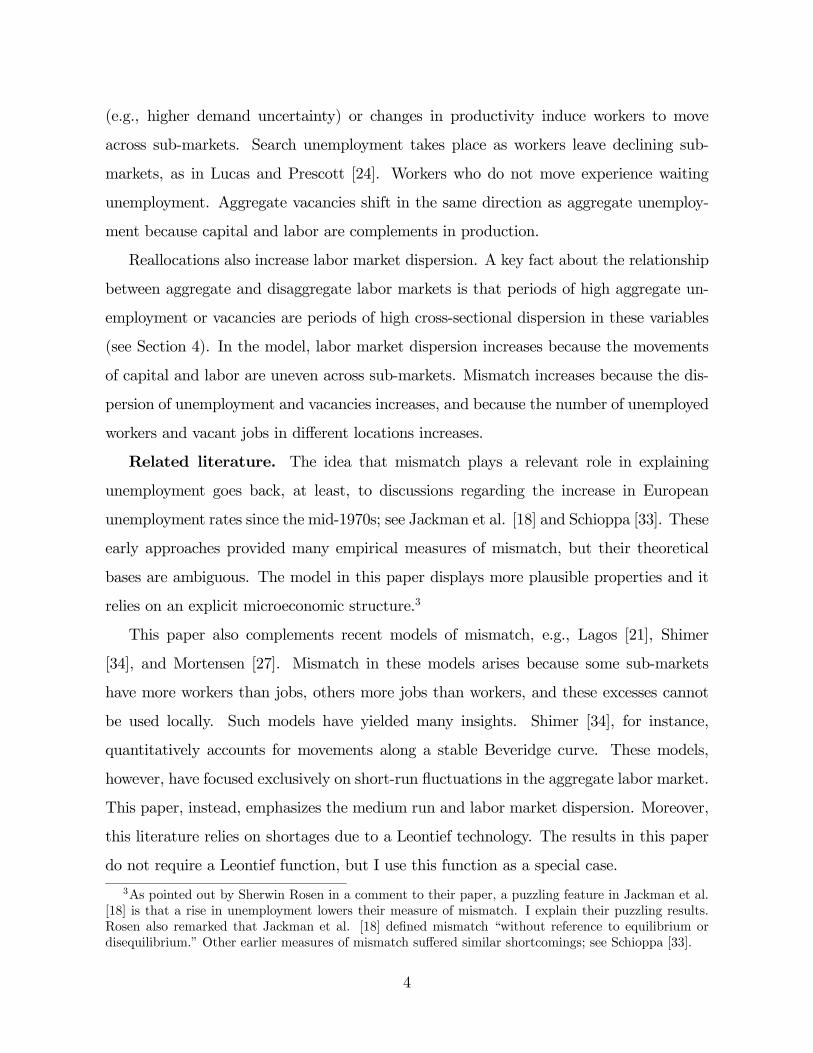
The quantitative significance of changes in the structure of labor markets is reflected

in the high volatility of the trend component of unemployment and vacancies, and in the

shifts in the Beveridge curve. As an illustration, Figure 1 displays the U.S. time series

of unemployment and vacancies and their trends obtained using the Hodrick-Prescott

filter. The trend components are as volatile as the cyclical components and the correla-

tion between trend components, 085, is precisely the opposite of the correlation between

cyclical components, −090. This strong positive correlation between medium-run trends1Many occupational, educational, and locational decisions are made with imperfect information about

the state of the labor market. In rural-urban migration models such as the Harris-Todaro model, workers

move to urban markets before knowing if they will be employed. This uncertainty is not captured by the

price uncertainty of search models or by a bilateral matching process. Moreover, typical labor markets

display a wide range of waiting activity enough to distinguish it conceptually from search; see, e.g., Jones

and Riddell [19].

2

1.5

2.0

2.5

3.0

3.5

4.0

4.5

5.0

1951 1959 1967 1975 1983 1991 1999 20070.5

1.0

1.5

2.0

2.5

3.0

3.5

4.0

ln(V) [left axis] ln(trend V) ln(U) [right axis] ln(trend U)

Figure 1: Postwar U.S. unemployment and vacancies, and medium-run trends, 1951-2007.

Trends based on a Hodrick-Prescott filter with a smoothing parameter of 100,000.

suggests shifts in the aggregate Beveridge curve.2 The 1950s and 1960s featured low

trend unemployment and vacancies. Most of the 1970s and 1980s featured high economic

volatility and high trend unemployment and vacancies. The 1990s and the early 2000s fea-

tured reduced economic volatility and low trend unemployment and vacancies. Economic

volatility appears to have increased in recent times. The Beveridge curve also appears to

have shifted recently; see, e.g., Daly et al. [14].

The theory provides an explanation for the changes in medium-run trends based on

capital and labor reallocations. In the model, resource reallocations are accompanied by

an increase in aggregate unemployment and vacancies. A decline in aggregate demand

2Abraham [2], Blanchard and Diamond [7], Bleakley and Fuhrer [9], Medoff [25], and Nickell et al.

[28] are some of the studies that have examined empirically the shifts in the Beveridge curve.

3

(e.g., higher demand uncertainty) or changes in productivity induce workers to move

across sub-markets. Search unemployment takes place as workers leave declining sub-

markets, as in Lucas and Prescott [24]. Workers who do not move experience waiting

unemployment. Aggregate vacancies shift in the same direction as aggregate unemploy-

ment because capital and labor are complements in production.

Reallocations also increase labor market dispersion. A key fact about the relationship

between aggregate and disaggregate labor markets is that periods of high aggregate un-

employment or vacancies are periods of high cross-sectional dispersion in these variables

(see Section 4). In the model, labor market dispersion increases because the movements

of capital and labor are uneven across sub-markets. Mismatch increases because the dis-

persion of unemployment and vacancies increases, and because the number of unemployed

workers and vacant jobs in different locations increases.

Related literature. The idea that mismatch plays a relevant role in explaining

unemployment goes back, at least, to discussions regarding the increase in European

unemployment rates since the mid-1970s; see Jackman et al. [18] and Schioppa [33]. These

early approaches provided many empirical measures of mismatch, but their theoretical

bases are ambiguous. The model in this paper displays more plausible properties and it

relies on an explicit microeconomic structure.3

This paper also complements recent models of mismatch, e.g., Lagos [21], Shimer

[34], and Mortensen [27]. Mismatch in these models arises because some sub-markets

have more workers than jobs, others more jobs than workers, and these excesses cannot

be used locally. Such models have yielded many insights. Shimer [34], for instance,

quantitatively accounts for movements along a stable Beveridge curve. These models,

however, have focused exclusively on short-run fluctuations in the aggregate labor market.

This paper, instead, emphasizes the medium run and labor market dispersion. Moreover,

this literature relies on shortages due to a Leontief technology. The results in this paper

do not require a Leontief function, but I use this function as a special case.

3As pointed out by Sherwin Rosen in a comment to their paper, a puzzling feature in Jackman et al.

[18] is that a rise in unemployment lowers their measure of mismatch. I explain their puzzling results.

Rosen also remarked that Jackman et al. [18] defined mismatch “without reference to equilibrium or

disequilibrium.” Other earlier measures of mismatch suffered similar shortcomings; see Schioppa [33].

4

The focus on labor market dispersion is clearly related to Lilien [23], although he

only examined cyclical unemployment; see Abraham and Katz [1] and Petrongolo and

Pissarides [30] for critical discussions of Lilien [23]. The idea that unused resources may

result from demand uncertainty is discussed in Prescott [32].4 The market decentralization

in this paper follows Eden [16]. In contrast to these papers, this paper is aimed directly

at examining worker-job mismatch.

The rest of the paper is as follows. Section 2 examines an economy without worker

mobility. Section 3 introduces worker search and capital accumulation. Section 3 also

discusses a numerical exploration of the general model under directed search, as in Lucas

and Prescott [24], and under random search, as in Alvarez and Veracierto [4]. Section

4 discusses the empirical relevance of the model and Section 5 presents some possible

extensions. Section 6 concludes. All technical proofs are in the Appendix.

2 The basic model

Environment. Time is discrete, indexed by ∈ 0 1 ∞. There is a continuum of

locations indexed by ∈ [0 1]. Each point represents a potential sub-market, not only ornecessarily a geographic location (i.e., skill, occupation, industry, or any combination of

these categories).

There is a measure one of workers in the economy. At the beginning of period ,

workers are attached to some location . Let () be the number of workers in and let

represent the distribution of workers across locations during period , e.g., ([0 1]) ≡Z 1

0

() = 1, by the previous convention. In the basic model, workers cannot move.

The next section allows worker movements which represent search.

There is a representative firm in each location. This firm has access to a production

function (() ()), which combines capital, (), and labor, (), to produce output.

(() ()) is increasing in () and (), has diminishing returns to scale, satisfies

4In Prescott [32], sellers of hotel rooms set prices before they know how many buyers will arrive. (In

Butters [10], sellers send price offers to potential costumers.) When the realization of demand is low,

rooms will remain vacant. Most existing studies focus on monopolistic pricing under demand uncertainty;

see, e.g., Bryant [11], Carlton [12], Dana [15], and Peters and Winter [29].

5

Inada conditions, and (() ()) 0. At the beginning of period , a location-

specific productivity shock, (), is realized. Productivity shocks are persistent but

independent across locations. The transition function for () is Markovian and has a

unique stationary distribution.

Aggregate demand is uncertain. There is a representative household made up of a large

number of individual members distributed along [0 1]. The preferences of the different

individual members differ and each member obtains utility from her own consumption

of goods. I assume, for simplicity, that utility is linear in consumption. There is a

continuum of possible demand states indexed by . Consumption in location and

state is ( ) ≡ ()( ), where () denotes the consumption per member

in and ( ) is the fraction of individual members that will arrive at the market

in . () is deterministic but ( ) is random. In particular, ( ) ∈ 0 1 isdriven by a preference shock to the marginal utility of consumption: ( ) ≡ min−() 0−(). This implies that consumers will only visit locations ≤ (),

e.g., ( ) = 1 if ≤ (), and ( ) = 0, otherwise. The random variable

() ∈ [0 1] thus determines the state of aggregate demand.Aggregate consumption is () =

Z 1

0

( ), where

( ) =

⎧⎨⎩ () if ≤ ()

0 otherwise.(1)

The objective of the representative household is to maximize E[()], where the

expectation is over possible realizations of the state .5

If demand is positive in , capital and labor are hired instantaneously and firms

produce to clear the goods market. To be hired, however, capital and labor must be

present in a given location. Capital is assigned before () is known. (In the general

5Individual demands may fluctuate stochastically as in Lucas and Prescott [24]. This alternative

source of uncertainty can be included in (1), but it does not contribute to the main points raised here.

The paper only requires that some locations face a positive probability of not producing. Other possible

assumptions such as technological obsolescence, an uncertain regulatory environment, or an uncertain

labor supply would, after appropriate modifications, yield equivalent results. The assumptions used here

highlight the role of changes in aggregate demand in generating output and unemployment.

6

model, worker movements will also take place before () is known.) This sequence of

events implies that there will be no excess capacity but that the capital and labor available

in locations () will remain idle. It is crucial that capital and labor cannot be

reassigned after () is realized. A sequential resolution of uncertainty in which some

sub-markets transact before others provides a rationalization of this assumption. I discuss

this point below.

Let ( ) denote the market-clearing level of output in location ,

( ) =

⎧⎨⎩ ()(() ()) if ≤ ()

0 otherwise.(2)

The structure of demand (1) implies that firms face a Bernoulli random variable: with

probability () ≡ Pr( : ≤ ()) production in takes place and with probability1− () ≡ Pr( : () ) no production occurs. These are the same probabilitiescapital and labor have of being hired. These probabilities and the shocks () are common

knowledge among workers and firms.

I assume that () is independently drawn each period. I retain the index in ()

to discuss the case of persistence in demand later on. Notice that () differs across

locations: (0) ≤ () for

0 ≥ . This order means that demand is “more uncertain”

for some firms. As expected, the volatility of output will be higher for firms with a

more uncertain demand. Differences in () and () will also support wage dispersion

in equilibrium. The special case when () is not indexed by does not particularly

simplify the analysis. As a drawback, this case assigns all heterogeneity across locations

to productivity differences.6

Finally, the total number of jobs is given by the economy’s total capital, . The

resource constraint for capital is

Z 1

0

() ≤ , (3)

6Discussing Lillien’s [23] analysis of unemployment, Abraham and Katz [1] argued that variations in

the cross-sectional distribution of unemployment could be driven by heterogeneous responses to aggregate

demand fluctuations. The function () implies a sectorally unbalanced response.

7

A planner problem. To maximize E[()], the (constrained) social planner must

assign capital () across locations knowing (), (), and (), but with no infor-

mation about (). Let ( ) be the value function of the planner problem. This

value function is the maximized expected aggregate output,

( ) ≡ max()

Z 1

0

E[( )], (4)

subject to (3) and the distribution of workers.7

Proposition 1 There exists a unique Pareto optimal capital assignment, and it is such

that capital is assigned to locations with a positive probability of production.

Proof. The proof is trivial. Let ∗ () be the optimal capital assignment. Then,

()()(∗ () ()) = . (5)

with as the Lagrange multiplier of (3), i.e., the opportunity cost of capital. By Inada

conditions, () 0 implies ∗ () 0.

Capital is assigned trading off its opportunity cost, , and the production probability,

(). A positive assignment of capital implies that the the expected marginal product of

labor in will be positive. It also implies that higher realizations of demand, i.e., a high

value of (), generate more capital and labor to be used and hence higher aggregate

output. These comparative statics, however, are not the focus of the paper. My focus is

on the long-run stationary allocation.

Recall (2) and let () be the mean of ( ). Then, () ≡ E[( )] =

()()(∗ () ()). The variance of the output produced in is [( )] ≡

E[(( )− ())2] = () [1− ()] ()(∗ () ())2, which follows due to the

Bernoulli all-or-nothing nature of demand.

Mean output and its variance are increasing in (), (), and (); see, e.g., (5).

The response in the variance of output to changes in () is, in general, ambiguous: a

7To avoid notational clutter, I omitted the terms () and (). Thus, ( ) is a short-handnotation for ( ; () ()∈[01]). Similar notation applies to the rest of the paper.

8

decline in () increases the variance directly but the decline in ∗ () lowers it. To resolve

the ambiguity, I assume that () ≥ 12 for all . At very fine levels of disaggregation,it is possible to find firms with low chances of selling their output. The fraction of idle

resources in the aggregate, however, appears to be small, e.g., () is likely to be close to

one. I also assume that the response in ∗ () to changes in () is “small.” To satisfy this

assumption, I assume throughout that −( )( ) ≥ q¯for q¯ 0. Conventional

concave functions satisfy this property. (An example that fails to do so is the linear

technology.) Under these assumptions, output dispersion in is decreasing in ().

Vacancies. The capital assigned to locations with no production will remain vacant.

Let ( ) denote job vacancies,

( ) =

⎧⎨⎩ ∗ () if ()

0 otherwise.(6)

Let () be the mean of ( ),

() ≡ E[( )] = [1− ()] ∗ (). (7)

The first term in the right-hand-side of (7) is the probability that no production takes

place, and the second is the assigned capital. The dispersion of vacancies is

[( )] ≡ E[(( )− ())2] = () [1− ()] ∗ ()2. (8)

The mean and variance of vacancies are ambiguous with respect to (). As the

Appendix shows, a bounded elasticity in the marginal product of capital resolves those

ambiguities:

Proposition 2 The mean number of job vacancies, (), and the dispersion of vacancies

are increasing in the productivity shock, (), and the number of workers, (); and

decreasing in the production probability, ().

These comparative statics follow from (5), (7), and (8), and are very intuitive.

9

Waiting unemployment. Let ( ) be the number of unemployed workers in given

. As in (6), ( ) = () if (), and ( ) = 0, otherwise. The mean number

of unemployed workers in , (), is

() ≡ E[( )] = [1− ()](). (9)

The interpretation of () is analogous to (7). Employment is ( ) ≡ () −( ), and its mean is E[( )] = ()(). The dispersion of unemployment,

which equals the dispersion of employment, is [( )] ≡ E[(( )− ())2] =

() [1− ()] ()2. The mean number of unemployed workers and the variance ofunemployment are both increasing in ().

Job “matches.” I treat capital in producing locations as being matched to employed

workers. Let () denote the mean number of job matches,

() ≡ E[∗ ()− ( )] = ()∗ (). (10)

The mean number of job matches is increasing in the productivity shock, the number

of workers, and the production probability. These predictions follow directly from (5) and

(10). Notice that changes in () do not generate an ambiguous response for (), and

that the dispersion of job matches is the same as the dispersion of vacancies, (8).

Discussion. It is not surprising that some capital and labor will remain idle when

decisions are made with imperfect information about the state of aggregate demand. The

significance of this result is that the model yields differences in mean unemployment and

vacancies across locations, and differences in their dispersion. These differences are consis-

tent with well-known observations.8 The model also implies that average unemployment

(and vacancies) and their dispersion should covary positively.

8Jackman et al. ([18], pp. 45) remarked that “as everybody knows, unemployment rates differ widely

between occupations and between regions, as well as across age, race and (sometimes) sex groups.”

Sherwin Rosen, in his discussion of mismatch, listed persistent differences in unemployment across skills

groups. Further, “employment and output variability are always greater in construction and in durable

goods manufactures than in services and non-durables manufacturing, and urban-rural and North-South

regional differences can persist for generations”; see Jackman et al. ([18], pp. 102).

10

To distinguish conceptually the unemployment that arises due to demand uncertainty

from search unemployment, I have used the notion of waiting unemployment. Waiting

unemployment captures the idea that workers enter the labor market before demand is

known. Since workers cannot immediately go to an alternative location if demand does

not arrive, workers have to wait out a spell of unemployment.

Jobs are divisible capital. This notion of a job is typical in business cycle models

(e.g., Cooley [13]), although it is slightly different from that used in existing models

of mismatch. Lagos [21], Shimer [34], and Mortensen [27] used a Leontief technology

( ) = min[ ]. If ( ) = min[ ], the planner solution is such that ∗ () = ()

given aggregate capital availability. In this case, capital may be unused due to a shortage

of workers, i.e., (6) becomes ( ) = max∗ ()− () 0 if () and ( ) = 0

otherwise. If 1, capital is in excess supply. On the other hand, if 1, there will

be an excess supply of labor in the least productive locations, i.e., workers in locations

with the lowest values of ()() will be in excess supply.9

The Leontief assumption provides a complementary reason for the existence of unused

capital and labor. Unemployment in the Leontief case is due to a shortage of jobs.

Unemployment here arises because there is no demand for the commodities certain workers

help produce. The difficulty here is not necessarily about job shortages in the local labor

market. In both cases, however, firms and workers will report unfilled vacancies and

unemployment when capital and labor are unused.

Shortages and the absence of factor substitution may be reasonable approximations in

the short term. Over a longer time period, allowing for factor substitution seems natural.

The Leontief assumption may also be restrictive empirically. If = 1 this assumption

implies () = (), see (7) and (9). Differences between local unemployment and

vacancies have in fact been previously used to measure matching inefficiencies; see, e.g.,

9Shimer [34] and Mortensen [27] considered a framework where capital and labor are assigned ran-

domly. There are no economic decisions regarding ∗ () or () in these papers. Factors are not assignedrandomly in Lagos [21], but he studied an inefficient allocation (see Section 5). The empirical distinction

between posted, filled, and unfilled job vacancies is not present in the theory. As in these previous models,

some locations have an “excess” of capital. This excess does not correspond to the traditional notion of

capital utilization, often viewed as an endogenous depreciation rate.

11

Schioppa ([33], pp. 11). In here, not all sub-markets should be equally “tight.”

Aggregation. The previous microeconomic structure can be easily aggregated. Ag-

gregate vacancies integrate (6), () =

Z 1

0

( ). Let ( ) be mean aggregate

vacancies,

( ) ≡Z 1

0

E[( )] =Z 1

0

(). (11)

The dispersion of aggregate vacancies will equal the aggregate over (8) if covariance

terms were zero. The Appendix shows that this approximation is valid when () is close

to 1. In that case,

[()] 'Z 1

0

[( )] =

Z 1

0

() [1− ()] ∗ ()2. (12)

Let ( ) be mean aggregate unemployment, ( ) ≡Z 1

0

E[( )]. The

dispersion of aggregate unemployment can be obtained as in (12). Mean aggregate job

matches integrate (10),

( ) =

Z 1

0

(). (13)

The degree of returns to scale in this “aggregate matching function” depends primarily

on the degree of returns to scale in the production function. The next proposition provides

a simple illustration:

Proposition 3 Suppose that ( ) has constant returns to scale. Then, ( ), has

constant returns to scale with respect to the mean number of unemployed workers, , and

vacant jobs, .

The proof is quite simple because unemployment is proportional to () and vacan-

cies and job matches are proportional to ∗ (). Notice that ( ) differs from the

conventional reduced-form aggregate matching function on which search and matching

models rely (e.g., Pissarides [31]). This literature focuses on the flow of aggregate job

matches given the stock of unemployed workers and vacant jobs. ( ) measures the

stock of aggregate job matches.

12

Mismatch. An immediate application is to compare mean individual and aggregate

outcomes in environments with different levels of uncertainty. Let an increase in demand

uncertainty be a first-order stochastic worsening in the distribution of(), e.g., a decline

in the production probabilities from () to 0() () for all ∈ [0 1]. An increase in

demand uncertainty represents a reduction in aggregate demand. (It can also be viewed

as a decline in aggregate total factor productivity since and are constant.)

Proposition 4 In response to an increase in demand uncertainty, mean individual and

aggregate unemployment and vacancies increase, and their individual and aggregate dis-

persion increases.

An increase in demand uncertainty increases mean unemployment and vacancies “every-

where.” The increase in mean unemployment and vacancies implies that higher demand

uncertainty “shifts” individual and aggregate Beveridge curves.10 These shifts are accom-

panied by higher dispersion in unemployment and vacancies.

An increase in the mean and the dispersion of labor market outcomes has been typ-

ically viewed as an increase in mismatch; see, e.g., Medoff [25], Jackman et al. [18],

Schioppa [33], and Petrongolo and Pissarides [30]. Higher demand uncertainty, however,

is only one of many possible causes of a simultaneous increase in means and dispersion.

In general, changes in productivity will also lead to resource reallocations that increase

unemployment, vacancies, and labor market dispersion. Further, in the basic model, un-

employed workers and vacant jobs are in the same locations. This feature is a consequence

of the absence of worker mobility. In the general model, workers searching for jobs and

vacant jobs will be in different places adding another dimension to mismatch. Finally, I

ignored the effects of changes in demand uncertainty on . The next section justifies this

omission.

The model also has measurement implications. To measure mismatch, Jackman et al.

([18], pp. 70) proposed an index based on the variance of relative unemployment rates,

10Petrongolo and Pissarides ([30], pp. 409) state that “in Britain the shifts in the regional Beveridge

curves were of the same order of magnitude as the aggregate curve, casting doubt on the power of

regional mismatch to explain the shift in the aggregate curve.” In here, individual and aggregate changes

in unemployment and vacancies are of similar orders of magnitude and, hence, consistent with this finding.

13

i.e., [( )()]. This index has been widely applied in the literature, but its

properties are not well-established. In this paper, [( )()] = ()()().

This index will not increase with a rise in demand uncertainty or in the unemployment

rate. In fact, both will yield a decline in the relative variance. These observations are

consistent with the puzzling finding of Jackman et al. [18] that measured mismatch fell

while unemployment rates increased in Europe. Their puzzling results can be understood

by taking into account that as () changes, the variance of unemployment will increase,

but it will not increase as fast as the mean.

The resolution of uncertainty. Thus far, decisions are made before any information

about demand is known. However, a partial revelation of information about demand

conditions will yield the same assignment of capital.

Assume capital assignments to 0 can be conditioned upon demand conditions in ,

with 0 . Let (0|) be the conditional probability of production in location 0,

given that production has taken place in . The benefit of assigning capital to 0 is

(0|)(0)((0) (0)), whereas the expected cost is (). Bayes’ rule implies

that conditioning on production in provides no incentive for reallocations to 0. The

intuition is simply that knowing demand conditions in provides no useful information

about the state of aggregate demand, (), which is the relevant source of uncertainty.11

Amarket assignment. There are multiple ways to model competitive markets under

demand uncertainty.12 I follow Eden [16] and consider competitive spot markets subject

to uncertain and sequential trade.

Agents know prices in all potential markets. The market for capital opens at the

beginning of each period, after () is known but before () is known. Workers supply

labor inelastically. Once capital and labor are decided, firms and workers just wait for

11Formally, (0|) ≡ Pr( : 0 ≤ ()| ≤ ()). Bayes’ rule yields (

0|)() =(|0)(0) = (

0) since (|0) = 1 as positive demand in 0 always implies positive demand in. The first order condition is: [(

0)()](0)(∗ (0) (0)) = (), which is (5). Landsburg

and Eden [22] and Peters and Winter [29] provide related remarks.12In the Arrow-Debreu model, a market in contingent claims would open before () is known and

claims would be redeemed after uncertainty is resolved. If decisions could be made contingent on (),there will be no unused factors. An alternative is to assume that firms post wages before () is known.Wages would remain fixed after uncertainty is resolved; see Prescott [32]. With pre-determined prices,

one needs to specify how rationing takes place as demand arrives; see, e.g., Dana [15].

14

the realization of demand. Demand arrives sequentially (but within a single period) and

its arrival triggers the opening of competitive goods and labor markets. All transactions

and production take place instantaneously. Markets then close. This process continues

until uncertainty is resolved. The number of markets that transact is greater the higher

the value of (). Since markets do not transact simultaneously, idle capital cannot be

reassigned to markets with positive demand because these markets already closed.

In a competitive market equilibrium, labor supply satisfies () = () if ()

0, where () is the wage rate in sub-market . Firms demand capital and labor to

maximize expected profits, ()()( ()

()) − ()

() −

(), where is

the rental price of capital. Factor markets clear: (3) holds, and () = (), for all

. (The distribution of profits does not affect the workers’ incentives and therefore is

not specified.) Equilibrium prices and quantities cannot be indexed by () because

information about () becomes available later in time.

The competitive equilibrium coincides with the solution to the social planner problem.

For example, the equilibrium rental price of capital coincides with . Under uncertain

and sequential trade, the equilibrium wage rate in is

() = ()()(∗ () ()). (14)

Wages are increasing in () and decreasing in (). Demand uncertainty also yields

equilibrium wage dispersion: sub-markets with a more uncertain demand exhibit higher

unemployment rates and lower wages.13

As in Prescott [32], the model does not feature the externalities typical of search

models, although they can be accommodated (see Section 5). In this economy, the markets

that transact always clear, and agents are price-takers and fully informed about potential

wages in the economy (e.g., there is no need to search). Under demand uncertainty,

however, not all markets transact in any given period.

13This implication is consistent with the fact that high-skilled workers typically have lower unemploy-

ment rates than low-skilled workers. Microeconometric earnings equations also show that workers in

labor markets with higher unemployment rates earn lower wages; see, e.g., Blanchflower and Oswald [8].

15

3 Capital accumulation and worker search

So far, aggregate capital is constant and workers are not able to leave their location. This

section allows for capital accumulation and worker search.

Capital accumulation. Capital accumulation decisions are made at the end of each

period, after the realization of demand. Let = ( −1) denote a history of demand

states. Aggregate consumption in period is (). The capital stock in period is

(−1), and the distribution of workers at the beginning of period is (

−1). Assume

for now that the law of motion of (−1) is deterministic. (This will be the case under

the conditions assumed below, but I will discuss the evolution of this distribution once I

discuss worker search.)

Initial capital 0 is given. Capital takes one period to enter production and it depre-

ciates at a constant rate ∈ (0 1). Unused capital also depreciates. Let ∈ (0∞) bethe time discount rate. The objective of the representative household is to maximize the

present discounted value of expected aggregate consumption, E0X∞

=0(1 + )−1(

),

where the expectation is over possible histories of realizations of the states . Since the

allocation of capital across locations takes place as in the basic model, and since utility

is linear, the objective of the representative household can be written simply as

max+1()

E0∞X=0

(1 + )−©((

−1) (−1))− [+1(

)− (1− )(−1)]

ª, (15)

where ((−1) (

−1)) is the value function of the static problem, see, e.g., (4).

The maximizing choice of +1() is characterized by the first order condition

E½+1(

∗+1(

) +1())

+1()

¾= + . (16)

The envelope theorem applied to the Lagrangian of the static problem, (4), yields

+1(∗+1(

) +1())+1(

) = +1(). Thus, for a given realization of de-

mand in period , the optimal capital accumulation plan equates the expected value

of the opportunity cost of capital in + 1, net of depreciation, to the discount rate, e.g.,

16

E[+1()] = + . The expectation term in (16) is relevant only if demand in period

yields useful information about demand conditions in + 1. Under the assumption that

() is independently drawn, +1() = () = (). Thus, the opportunity cost of

capital in + 1 will equal + regardless of the demand conditions in .

The aggregate state of the economy is ((−1) (

−1)). In equilibrium, factor

prices depend on the aggregate state. This dependence means that workers, when making

search decisions, would need to predict how changes in the aggregate capital stock and in

the distribution of workers influence future wages. The main advantage of assuming that

() is independently drawn each period is that the opportunity cost of capital will be in-

dependent of the aggregate state. Wages will also be independent of ((−1) (

−1)).

In this case, search decisions will only be based on location-specific variables. This implies

that I can examine a stationary solution based on a “representative island.”

The independence assumption in aggregate demand and the independence in produc-

tivity shocks across locations also imply that there is no aggregate uncertainty. Therefore,

in the solution of the dynamic problem analyzed later in this section, the sequence is deterministic. (In the Appendix I show formally that +1 evolves deterministically.)

In the stationary allocation, the aggregate capital stock will be a stationary point, ∗,

and that the distribution of workers will be a stationary distribution, ∗.14

Worker search. Workers are initially distributed according to 0. Workers are al-

lowed to move between locations after observing (), but before () is known.15

Movements are of two types: the variable () represents workers who move out of ,

i.e., searchers. The variable () represents workers who move in, i.e., worker arrivals.

The purpose of worker search is to find the distribution of workers that maximizes (15),

given 0 and the search technology specified below. I assume that worker search and

14If demand is persistent, the solution will involve a stationary distribution of aggregate capital and

a distribution over the distribution of workers. Aggregate capital converges to a stationary point under

i.i.d. shocks even under convex adjustment costs. Under adjustment costs, however, workers would need

to use the aggregate capital stock in their decision-making process. The aggregate capital stock and the

distribution of workers are not relevant in Lucas and Prescott [24] since they do not allow for capital

mobility.15As in the basic model, if partial information about demand is available, all the results remain un-

changed.

17

capital assignments are simultaneously decided.

Search is costly because searchers cannot work for one period, while in transit. Given

the number of workers who stay in , ()− (), employment is

( ) =

⎧⎨⎩ ()− () if ≤ ()

0 otherwise.(17)

As in the basic model, if demand is positive in , all available workers, () − (),

will be employed. The number of workers in evolves as

+1() = () + ()− (). (18)

Feasibility in worker search requires that the total number of workers searching be

equal to the total number of arrivals so that +1([0 1]) ≡Z 1

0

+1() = 1. That is,

Z 1

0

() =

Z 1

0

(). (19)

Solution. The solution to the dynamic assignment problem consists of a bounded

sequence of aggregate capital that maximizes (15). It also involves a bounded sequence

of the distribution of workers consistent with the law of motion generated by worker

search. For a given aggregate capital and a given distribution of workers, the capital

assignments to each location take place as in the basic model. The only difference is

that some workers may leave the location. The rest of this section examines the social

planner solution of the dynamic assignment. The solution to the social planner’s dynamic

problem will also be a competitive equilibrium.

Aggregate capital satisfies (16). Thus, aggregate capital will be such that = +

for all ≥ 1.16 Capital assignments across locations are analogous to those described by(5), and hence they do not require any further comment. Search decisions involve two

16I have ignored the case where + even if all output is saved. If initial capital is too low, the

representative household will choose to save all output until = + , which will happen in finite time.

For the results presented here, it is only necessary that this equality holds in the stationary case.

18

choices in each location: () and (). Let ∗ () and ∗ () be the optimal number of

workers who search and arrive at location , respectively. Let ∗+1() be the number of

workers in location once searchers arrive, just before the beginning of the next period.

I consider a directed search assignment where workers direct their search to the most

attractive locations. In a numerical analysis below, I examine random search based on

the specification used by Alvarez and Veracierto [4]. Under random search, the arrival of

workers will be independent of , e.g., () = for all .

To save on notation, let () be the expected marginal product of labor in ,

() = ()()(() ()− ()). (20)

() is also the equilibrium wage rate under uncertain and sequential trade, (14). The

marginal product of labor depends on capital and it takes into account the fact that some

workers may leave the location. Expected wages in sub-market and period + 1 are

E[+1()], where the expectation is taken over the location-specific productivity shock,

+1(), which is unknown at the time search decisions take place. (The expectation over

demand conditions, e.g., (), is already included in +1().)

Let denote the Lagrange multiplier for the constraint (19), i.e., the opportunity cost

of search. Since the aggregate state evolves deterministically, is deterministic. Optimal

search decisions involve two separate Euler equations. Worker search satisfies

µ − ()− E[+1()]

1 +

¶∗ () = 0, (21)

where the term in parentheses equals zero if ∗ () 0. Worker arrival satisfiesµE[+1()]

1 + −

¶∗ () = 0, (22)

where the term in parentheses equals zero if ∗ () 0.

To understand the implications of (21) and (22), it is useful to consider the three

standard cases that characterize worker search; see Lucas and Prescott [24] and Stokey,

19

Lucas, and Prescott ([35], section 13.8):

(i) Workers leave , i.e., ∗ () 0 and ∗+1() = () − ∗ (). Thus, search takes

place up until the point in which the workers who stayed behind are indifferent between

staying and searching.

(ii) No additional worker arrives and no worker leaves , i.e., ∗ () = ∗ () = 0

and ∗+1() = (). Workers in these locations are not willing to forego their current

expected payoff in order to search. The distribution of workers in these locations remains

unchanged.

(iii) Workers arrive in , i.e., ∗ () 0 and ∗+1() = () + ∗ (). Since search is

directed, these workers are assigned in such a way that the expected payoff from searching

is equalized across locations (i.e., until the term in parentheses in (22) holds with equality).

The next proposition addresses the existence and uniqueness of a stationary solution

to the dynamic assignment problem. A stationary allocation is a vector (∗ ∗) such that

= ∗, and = ∗. A stationary allocation also involves a series of functions describing

the number of searchers and arrivals to each location, ∗ () = ∗() and ∗ () = ∗()

respectively, and the capital assignment, ∗ () = ∗(). These functions depend on the

opportunity cost of capital, + , and on the state of each sub-market, e.g., the number

of workers at the beginning of the period, (), and the augmented shock, ()().

Proposition 5 For a given initial capital stock and a distribution of workers (0 0),

there exists a unique stationary solution to the dynamic assignment problem.

Proof (Idea). The idea is that a stationary version of the dynamic assignment

problem can be studied along the lines considered by Lucas and Prescott [24].

Let () ≡ ()() denote an augmented shock in . Let

(() ()) ≡ max()

()(() ())− (+ )().

This indirect production function nets out the effect of capital mobility. Thus, search

decisions can be made on the basis of the function (() ()) alone, which only de-

pends on the state of the local labor market, () and (). Since worker search and

20

capital assignments are simultaneously decided, capital will change optimally in response

to workers leaving location . The rest of the proof involves showing that the function

(() ()) satisfies the assumptions in Lucas and Prescott [24] and that the stationary

allocation has their recursive representation.

Discussion. Equilibrium search models typically abstract from capital mobility and

capital accumulation; see, e.g., Lucas and Prescott [24], Gouge and King [17], Alvarez and

Shimer [5]. The use of the indirect production function (() ()) provides a simple

and tractable way to incorporate a firm’s choice of capital as well as factor substitution

into models of equilibrium search.

Proposition 5 only relies on differentiability and concavity properties on (() ()).

Consider, for example, the case of a Cobb-Douglas production function, (() ()) =

()() with + 1. The indirect production function satisfies

(() ()) = ()1(1−)[(+ )](−1)()(1−). (23)

Proposition 5 also holds under a Leontief production function. Assume, for example,

that (() ()) = min[() ()] with ∈ (0 1). The indirect production functionwill simply be (() ()) = ()(). The stationary value of the capital stock, ∗, is

such that the capital-labor ratio will equal one for all potentially employed workers, e.g.,

∗ =Z 1

0

[∗()−∗()]. In this case, the stationary allocation involves no excess supplyof capital (or labor) such as that possible in the basic model under a Leontief production

function. In the basic model, the aggregate capital stock was a given parameter, whereas

here ∗ is optimally chosen.

The function (() ()) can be used to highlight important differences with existing

search models. In models without capital, a large number of workers lowers equilibrium

wages and induces workers to search. When capital is movable, and labor and capital are

complements, a large number of workers is an incentive for capital flows. Capital in-flows

increase wages even if workers do not search. Thus, abstracting from capital mobility

will likely overstate the importance of search unemployment. On the other hand, capital

mobility amplifies the effect of shocks (). For example, the exponent on () in (23),

21

1(1−), is larger than one. The reason is that a good location (e.g., a location with highvalues of ()) attracts workers and capital directly, but also indirectly as both factors

are complements. Thus, capital mobility will likely make wages more unequal increasing

the benefit of search.

Search provides other insights as well. Worker search is decreasing in the augmented

shock, (); see Lucas and Prescott ([24], Proposition 2) and Stokey, Lucas, and Prescott

([35], section 13.8). This implies that search is lower in more productive locations but also

in locations with less uncertain demand, e.g., workers search to “insure” against demand

uncertainty. Since the arrival at a new location does not guarantee employment, even is

search is directed, this insurance is limited. Another consequence of this result is that

workers will differ in the duration of their unemployment spells. (In Lucas and Prescott

[24], all unemployment spells are of the same length.)

The theory also predicts that worker reallocation will take place slowly over time.

While I do not examine the speed of adjustment to the “steady state,” transitions are

likely to be slow.17 Notice also that sub-markets with a high fraction of searchers are

sub-markets with fewer vacancies and job matches. This result follows from Proposition

2: ∗() satisfies ()(∗() ∗()−∗()) = + . Since ( ) 0, as workers leave,

the expected marginal product of capital in that sub-market declines. This implies that

∗() is decreasing (parametrically) in ∗(), and (7) and (10) imply fewer vacancies and

job matches.

The mean and variance of output, unemployment, vacancies, and job matches are

characterized as in the basic model. For example, mean unemployment in is ∗() =

∗() + (1 − ())[∗() − ∗()]. The first component is due to search frictions and the

second to demand uncertainty, e.g., waiting unemployment. The variance of unemploy-

ment is () [1− ()] ∗() − ∗()2, which, parametrically speaking, is a decreasingfunction of ∗(). In the general model, mean and variance are also positively related,

but the relationship is weaker than in the model without search because search reduces

17Stokey, Lucas, and Prescott ([35], section 13.8b) best illustrate this point through the less-than-

unitary slope of the policy function with respect to changes in the number of workers at the beginning

of the period.

22

the dispersion of unemployment across sub-markets. Aggregate labor market outcomes

can also be obtained as in the basic model.

Finally, notice that searchers are not attached to any particular sub-market. The

search technology prevents workers from using the vacant jobs. Thus, searchers and

vacant jobs are in different places, e.g., mismatched.

Numerical results. In this sub-section I obtain some numerical solutions for the

above model. The main purpose of these exercises is to examine how the mean and

cross sectional distribution of output, unemployment, and vacancies change in response

to changes the technological and demand conditions of the economy.

The model can be parameterized easily. I assume an exponential distribution for(),

i.e., () = 1 − exp−. Productivity shocks are given by () = −1() exp,with 2 as the variance of . The variance of log-productivity is

2(1 − ). Thus, an

increase in 2 and make ()more volatile. I use the Cobb-Douglas production function

consistent with (23). I consider each period to be a quarter. The time discount rate is

= 104514− 1, and the depreciation rate is = 0012. I assume = 060 and = 095.

These measures are conventional values in real business cycle models; see, e.g., Cooley

([13], pp. 22). For the volatility parameter, I use = 010, which is roughly the value

used by Alvarez and Veracierto ([4], Table 1). I assume that = 010. Under a value of

= 005, 2.9 percent of the capital stock remains vacant.18

Table 1 reports the baseline results under directed search. Panel A reports the station-

ary mean values of labor market outcomes, capital, and output. In the baseline case, total

vacancies (measured as a fraction of the capital stock) are 292 percent, whereas the total

unemployment rate is 405 percent. Search unemployment is 120. Waiting unemploy-

ment is 285. The opportunity cost of search, , is about four times output per worker.

The stationary value of the capital-output ratio is 5. Panel B uses the endogenous distri-

bution of workers across locations to obtain aggregate measures of dispersion for output,

employment, total unemployment, and vacancies. The specific numerical values in Panel

B are not important. The most relevant aspect in Panel B is the direction of change

18The solution is based on a value function iteration with bounds for the employment grid that ensure

that there is a unique invariant distribution, see Stokey, Lucas, and Prescott ([35], section 13.8).

23

across specifications.

Table 1. Numerical simulations under directed search.

Alternative parameter values

(1) (2) (3)

Baseline = 0.9875 = 0.20 = 0.10

A. Stationary mean values

Total unemployment rate 4.05 5.47 7.20 6.98

Search unemployment 1.20 1.84 3.85 1.36

Waiting unemployment 2.85 3.63 3.35 5.62

Vacancy rate 2.92 3.38 3.21 5.74

Cost of search 0.72 1.16 1.05 0.71

Capital per worker 0.91 1.10 1.16 0.81

Output per worker 0.18 0.21 0.23 0.16

B. Cross-sectional variance

Output 0.0021 0.0072 0.0079 0.0028

Employment 0.0499 0.2032 0.1708 0.0871

Unemployment 0.0084 0.0335 0.0439 0.0545

Vacancies 0.0081 0.0310 0.0498 0.0405

Note.— The mean values and the cross-sectional variances are constructed using the stationary

distribution of workers. The unemployment and vacancy rates are in percent.

Table 1 also studies the effects of changes in the structural characteristics of the

economy. The first alternative specification, (1), increases the persistence of the location-

specific productivity shocks from = 095 to = 09875, which is roughly the value

used by Alvarez and Veracierto ([4], Table 1). The table shows that the two forms of

unemployment increase. Higher persistence in the productivity shock also leads to higher

capital accumulation, a higher vacancy rate, and higher output.

There are two reasons behind these changes. First, when persistence increases, a high

realization of productivity in the present period increases the chances of a high realization

of productivity in the future. As a consequence, expected wages increase and this makes

worker search more attractive. To understand the reasons behind the increase in waiting

unemployment, it is useful to first examine the changes in aggregate capital. Aggregate

capital increases because an increase in persistence also raises the future expected marginal

24

product of capital. This change is an intertemporal incentive to accumulate more capital.

To understand the changes in vacancies, notice that when the aggregate capital stock

is low, capital should be concentrated in locations with low demand uncertainty, e.g.,

locations more likely to produce. As aggregate capital increases, more capital is assigned

to locations with more uncertain demand. This explains why the vacancy rate increases.

Finally, since capital and labor are complements, as more capital is assigned to locations

with more uncertain demand, more workers will also locate in these locations (relative to

the baseline case). These workers will be more likely to experience waiting unemployment.

Notice that higher persistence is an incentive to locate in locations with more uncertain

demand, but also an incentive for higher mobility.

There is a second reason behind the changes in (1). An increase in persistence of

productivity makes () more volatile. Higher volatility makes wages more unequal and

this gives workers more incentives to search. The marginal product of capital will also be

more unequal across locations. These changes also lead to capital and labor reallocations

to locations with more uncertain demands.

The second specification, (2), increases the volatility of location-specific productivity

shocks from = 010 to = 020. Higher dispersion in the productivity shocks also

increases unemployment, and it leads to higher capital accumulation and a higher vacancy

rate. Quantitatively, the effects on capital, vacancies, and output are similar to those of

specification (1). An increase in the volatility of the shocks leads to higher cross-sectional

dispersion in wages and the marginal product of capital. The main difference between (1)

and (2) is that search unemployment increases more in response to changes in than to

changes in .

The previous exercises consider resource reallocations driven by technological factors,

e.g., changes in the stochastic process that governs (). The last exercise, (3), considers

a decline in aggregate demand or a rise in demand uncertainty, as in Proposition 4. I

increase from = 005 to = 010. Under higher demand uncertainty, unemployment

and vacancies also increase. The main component behind the increase in unemployment is

waiting unemployment, although search also becomes more attractive. The logic behind

25

these changes is that of the basic model. A decline in () increases waiting unemployment

and vacancies directly. Since workers search partly to “insure” against an uncertain

demand, search unemployment also increases. In response to a shift in (), vacancies

increase but the aggregate capital stock and total output decline. The decline in mean

aggregate capital and output contrasts with the increase in these variables in specifications

(1) and (2).

Panel B displays the microeconomic dispersion associated with the previous specifica-

tions. In all cases, the increase in mean unemployment and vacancies seen in Panel A are

accompanied by an increase in the cross-sectional dispersion of these variables. These re-

sults are consistent with Proposition 4. Notice that the dispersion of output also increases

in these specifications.

Overall, the labor market adjustments in specifications (1) to (3) are associated with

“shifts” in the stationary values of unemployment and vacancies compared to the baseline

case. There are obvious differences in terms of which type of unemployment contributes

more to the increase in total unemployment, and differences in whether the shifts are pro-

or counter-cyclical. However, a process of resource reallocation increases unemployment

and vacancies. Since the number of workers searching and the number of vacant jobs

increase, and since searchers and vacancies are in different locations, mismatch increases

in this dimension. These reallocations are also associated with higher overall labor market

dispersion, which is another dimension of mismatch.

Table 1 uses a directed search specification. Table 2 reproduces Table 1 under random

search, as considered in Alvarez and Veracierto [4]. I maintain all parameter values as in

the numerical simulations of Table 1. Under random search, the Euler equation (21) also

holds but the arrival of workers in (22) is not directed. Instead, () = for all ∈ [0 1].The law of motion (18) and the feasibility condition (19) change accordingly.

There are two noticeable aspects in Table 2. First, search unemployment is higher

under random search than under directed search. Notice, however, that there are no

significant differences in the opportunity cost of search. The reason is that under directed

or random search, the decision to leave a location is based on the same Euler equation,

26

(21). The second noticeable feature is that random search causes capital and output to

be considerably lower in Table 2 relative to Table 1. The reason is that random search

induce more worker and capital mobility than directed search.

Table 2. Numerical simulations under random search.

Alternative parameter values

(1) (2) (3)

Baseline = 0.9875 = 0.20 = 0.10

A. Stationary mean values

Total unemployment rate 5.90 12.29 14.03 6.98

Search unemployment 3.21 8.99 11.06 3.07

Waiting unemployment 2.69 3.30 2.97 5.27

Vacancy rate 2.49 2.78 3.21 4.88

Cost of search 0.75 1.18 1.09 0.72

Capital per worker 0.39 0.56 0.59 0.39

Output per worker 0.08 0.11 0.11 0.07

B. Cross-sectional variance

Output 0.0001 0.0005 0.0003 0.0002

Employment 0.0073 0.0164 0.0111 0.0140

Unemployment 0.0012 0.0050 0.0057 0.0083

Vacancies 0.0003 0.0038 0.0033 0.0021

Note.— The mean values and the cross-sectional variances are constructed using the stationary

distribution of workers. Random search is based on the specification in Alvarez and Veracierto

[4]. The unemployment and vacancy rates are in percent.

Despite the previous differences, the labor market adjustments share the features seen

in Table 1. The process of resource reallocation in specifications (1) to (3) increases

unemployment and vacancies (e.g., the Beveridge curve shifts). Labor market dispersion

also increases during these reallocations. Thus, the conclusions obtained under directed

search appear to be robust to the alternative random search protocol.

4 Some implications of the theory

This section examines the implications of the theory for the medium-run behavior of

aggregate unemployment and vacancies, and for the dispersion of labor market outcomes.

27

The Beveridge curve. I first examine the “medium-run Beveridge curve.” I use

seasonally adjusted unemployment rates from the Bureau of Labor Statistics (BLS). To

measure vacancies, I use the Conference Board help-wanted advertising index, the best

available U.S. vacancy rate proxy prior to 2000. After December 2000, I use the job

openings rate from the Job Openings and Labor Turnover Survey (JOLTS). The vacancy

index is re-scaled using periods of common overlap.19

Table 3 estimates the trend components of unemployment and vacancies for alternative

sample periods. Panel A starts in the first quarter of 1951 and ends in the last quarter of

1997. The help-wanted index has declined since the mid-2000s due to online job posting

and the use of other recruitment methods. The sample in Panel A is not influenced by

these changes in advertisement or by potential problems due to the merging procedure

with JOLTS. Panel B ends in the last quarter of 2007 (before the 2007-2009 recession).

Because filtering for medium-run trends is sensitive to end points, this sample period

provides results that are not affected by the sharp rise in unemployment during the 2007-

2009 recession. Panel C includes data up until the last quarter of 2010.

Table 3 decomposes unemployment and vacancies using the Hodrick-Prescott (HP) fil-

ter, the Baxter-King (BK) filter, and a third-degree polynomial in time. With a smoothing

parameter of = 0, the HP filter returns the raw data. I focus on Panel B. These results

are virtually identical to those in Panel C. The results in Panel A provide stronger support

for the points discussed here.

Table 3 suggests two basic points: (i) The trend components of unemployment and

vacancies are as volatile as the cyclical components. Under the HP filter with = 10 000,

the standard deviation of the trend components is about 75 percent of the standard

deviation of the raw series. These values are similar to those in the BK filter. Under

= 100 000, the standard deviation of the trend component of unemployment is of

the same order of magnitude as the standard deviation of the cyclical component. (A

third-order polynomial in time yields similar results.) Under = 150 000, the standard

deviations are also of similar magnitudes.

19Unemployment rates are available in www.bls.gov. I would like to thank Ken Goldstein for makinghelp-wanted advertising index available. JOLTS is also available from the BLS.

28

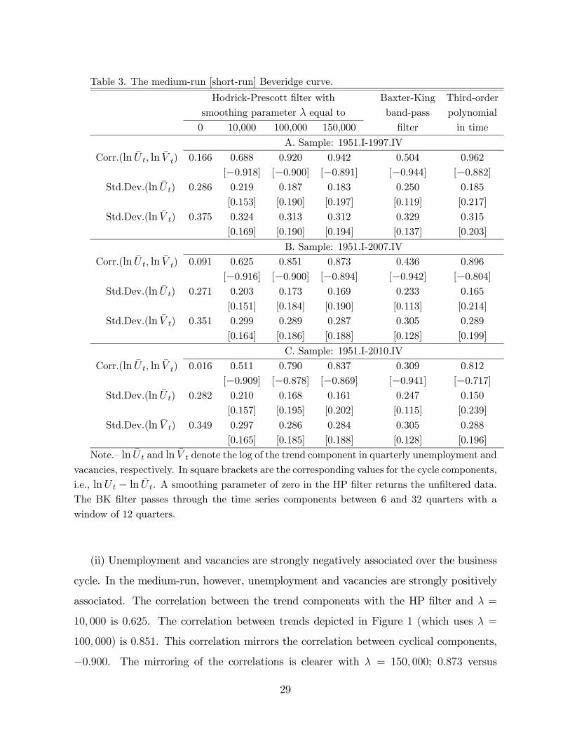
Table 3. The medium-run [short-run] Beveridge curve.

Hodrick-Prescott filter with Baxter-King Third-order

smoothing parameter equal to band-pass polynomial

0 10,000 100,000 150,000 filter in time

A. Sample: 1951.I-1997.IV

Corr.(ln ln ) 0.166 0.688 0.920 0.942 0.504 0.962

[−0.918] [−0.900] [−0.891] [−0.944] [−0.882]Std.Dev.(ln ) 0.286 0.219 0.187 0.183 0.250 0.185

[0.153] [0.190] [0.197] [0.119] [0.217]

Std.Dev.(ln ) 0.375 0.324 0.313 0.312 0.329 0.315

[0.169] [0.190] [0.194] [0.137] [0.203]

B. Sample: 1951.I-2007.IV

Corr.(ln ln ) 0.091 0.625 0.851 0.873 0.436 0.896

[−0.916] [−0.900] [−0.894] [−0.942] [−0.804]Std.Dev.(ln ) 0.271 0.203 0.173 0.169 0.233 0.165

[0.151] [0.184] [0.190] [0.113] [0.214]

Std.Dev.(ln ) 0.351 0.299 0.289 0.287 0.305 0.289

[0.164] [0.186] [0.188] [0.128] [0.199]

C. Sample: 1951.I-2010.IV

Corr.(ln ln ) 0.016 0.511 0.790 0.837 0.309 0.812

[−0.909] [−0.878] [−0.869] [−0.941] [−0.717]Std.Dev.(ln ) 0.282 0.210 0.168 0.161 0.247 0.150

[0.157] [0.195] [0.202] [0.115] [0.239]

Std.Dev.(ln ) 0.349 0.297 0.286 0.284 0.305 0.288

[0.165] [0.185] [0.188] [0.128] [0.196]

Note.— ln and ln denote the log of the trend component in quarterly unemployment and

vacancies, respectively. In square brackets are the corresponding values for the cycle components,

i.e., ln − ln . A smoothing parameter of zero in the HP filter returns the unfiltered data.

The BK filter passes through the time series components between 6 and 32 quarters with a

window of 12 quarters.

(ii) Unemployment and vacancies are strongly negatively associated over the business

cycle. In the medium-run, however, unemployment and vacancies are strongly positively

associated. The correlation between the trend components with the HP filter and =

10 000 is 0625. The correlation between trends depicted in Figure 1 (which uses =

100 000) is 0851. This correlation mirrors the correlation between cyclical components,

−0900. The mirroring of the correlations is clearer with = 150 000; 0873 versus

29

−0894. Panel A, provides an even sharper contrast of the correlations of medium-runtrends and the correlation of the cyclical components.

The main implication of (i) is that a significant fraction of the volatility of unem-

ployment and vacancies is due to fluctuations in their medium-run trends rather than

to fluctuations in their business cycle components. Consistent with (i), the focus of the

theory has been on stationary allocations and on how resource reallocations affect the

stationary values of unemployment and vacancies.

In terms of (ii), notice that during a business cycle, unemployment and vacancies

move along the Beveridge curve; see, e.g., Shimer [34]. However, the strong positive

correlation between medium-run trends shows that the Beveridge curve itself tends to

shift. Although (ii) is sensitive to the smoothing procedure, its main implication is that

the medium-run Beveridge curve is positively sloped. This finding is important because

a negatively sloped Beveridge curve has been used as evidence against the importance of

labor market imbalances or mismatch; see, e.g., Abraham and Katz ([1], pp. 513-515),

Schioppa ([33], pp. 17-19), and Petrongolo and Pissarides ([30], pp. 400).

The focus of the existing literature on unemployment and vacancies has been almost

exclusively on business cycle frequencies.20 Empirically, (ii) suggests that resource real-

locations have the greatest impact on labor markets at time scales longer than those of

a business cycle. To explain a positively sloped medium-run Beveridge curve, the the-

ory essentially posits the need to reallocate both capital and labor from declining firms.

As Proposition 4 suggests for the basic model, and as illustrated in Tables 1 and 2, the

complementarity between capital and labor implies that the stationary values of unem-

ployment and vacancies increase due to reallocations driven by changes in productivity

or by changes in demand uncertainty.

There are several difficulties with the measurement of unemployment and vacancies

(e.g., the help-wanted index). Table 3 shows that removing recent observations, which

are subject to changes in advertisement technologies, yields stronger results. Medoff [25]

20Blanchard and Diamond [7] is an important exception. They argue that half of the shifts in the

Beveridge curve are due to reallocation shocks, and the other half are “due to an unexplained deterministic

trend,” Blanchard and Diamond ([7], pp. 4-5). During the 1990s and until 2007, medium-run trends for

unemployment and vacancies declined jointly. This decline is not consistent with a deterministic trend.

30

2

3

4

5

6

7

8

9

10

11

12

Jan-74 Jan-79 Jan-84 Jan-89 Jan-94 Jan-99 Jan-04 Jan-091

2

3

4

5

6

Unem ploym ent rate [left axis ]

Cross-sectional dispers ion of unem ploym ent across 13 industries [right axis ]

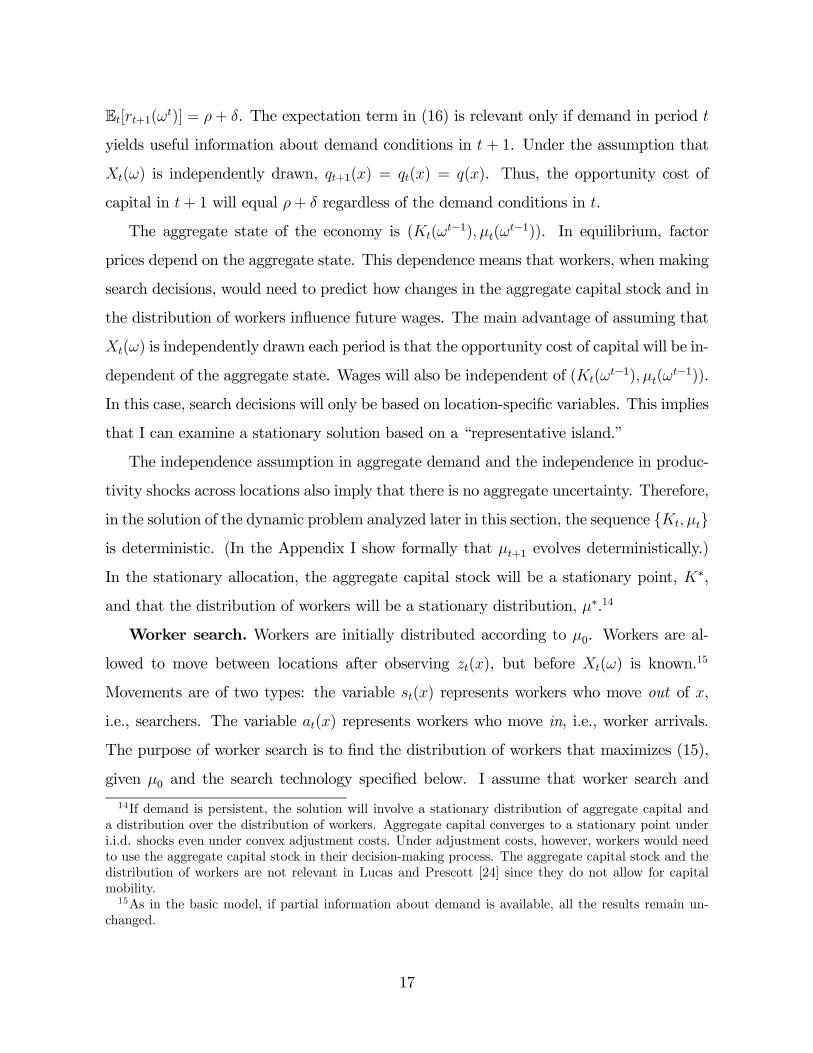
Figure 2: Unemployment and cross-sectional dispersion of unemployment.

has shown that the shifts in the U.S. Beveridge curve in the 1970s are supported by cross-

sectional evidence and by evidence based on discharges and quits. See also Abraham [2],

Blanchard and Diamond [7], Bleakley and Fuhrer [9], and Daly et al. [14] for additional

evidence on the shifts in the Beveridge curve. Further, the majority of Western European

countries have experienced multiple shifts in the Beveridge curve during the post-war

period. With the exception of Norway and Sweden, the Beveridge curve shifted to the

right by a sizable amount from the 1960s to the early 1980s; see, e.g., Nickell et al. ([28],

Figure 1). This shift is similar to that evident in Figure 1.

Labor market dispersion. The model implies that resource reallocations will not

only increase unemployment and vacancies, but also lead to higher labor market dis-

persion. In this sub-section, I examine empirically the association between means and

dispersion for unemployment and vacancies.

Figure 2 displays the unfiltered monthly unemployment rate and the standard devi-

31

ation of unemployment rates across 13 industries, .21 As the figure shows, the unem-

ployment rate and its cross-sectional dispersion are strongly positively related: periods of

high unemployment are periods of high dispersion in the cross-section of industries.

Table 4. Correlation between mean unemployment and its dispersion.

Lilien’s [23] Cross-sectional dispersion of

dispersion index unemployment

ln ln ln ln lnln 1.000 0.645 0.966 0.957 0.927

[0.534] [0.878] [0.775] [0.390]

ln 1.000 0.666 0.600 0.535

ln 1.000 0.972 0.935

ln 1.000 0.958

ln 1.000

Groups 13 13 11 50

Obs. 456 418 418 419

[420] [384] [384] [384]

Note.— () denotes Industries, () Occupations, and () States. Lilien’s ([23], 787) index of

employment dispersion uses monthly data from the “Current Employment Statistics” program

of the BLS since January, 1973 and expresses monthly growth rates relative to 12 months earlier.

The dispersion of unemployment measures the standard deviation of unemployment rates since

January, 1976. Unemployment dispersion measures use microdata from the CPS. In square

brackets are the values for samples that end before December, 2007.

The strong positive association between means and dispersion in Figure 2 is not lim-

ited to the dispersion across industries. Table 4 displays the correlations between the

unemployment rate and several measures of labor market dispersion. Given the reduced

availability of dispersion measures for vacancies, my main focus is on unemployment rates.

Table 4 uses monthly data until December 2010. The values in square brackets are based

on the sample that ends in December, 2007.

21The underlying data used for measures of dispersion are the monthly files of the Current Population

Survey (CPS), available since January, 1976. Dispersion measures are calculated based on workers char-

acteristics prior to the current unemployment spell. I would like to thank Rob Valletta and Katherine

Kuang from the Federal Reserve Bank of San Francisco for making these data available; see Daly et al.

[14] for additional information about these data.

32

The most salient feature of Table 4 is the strong positive correlation between aggre-

gate unemployment and its cross-sectional dispersion across industries, occupations, and

states. Table 4 also shows a positive correlation between all measures of unemployment

dispersion. For example, Lilien’s [23] index of employment growth dispersion is posi-

tively correlated with the aggregate unemployment rate. (Lilien’s [23], however, index

is negatively correlated with the unfiltered aggregate vacancy rate, as first documented

by Abraham and Katz [1].) The fact that multiple measures of unemployment disper-

sion are positively associated suggests that labor market dispersion typically increases

simultaneously along multiple dimensions.

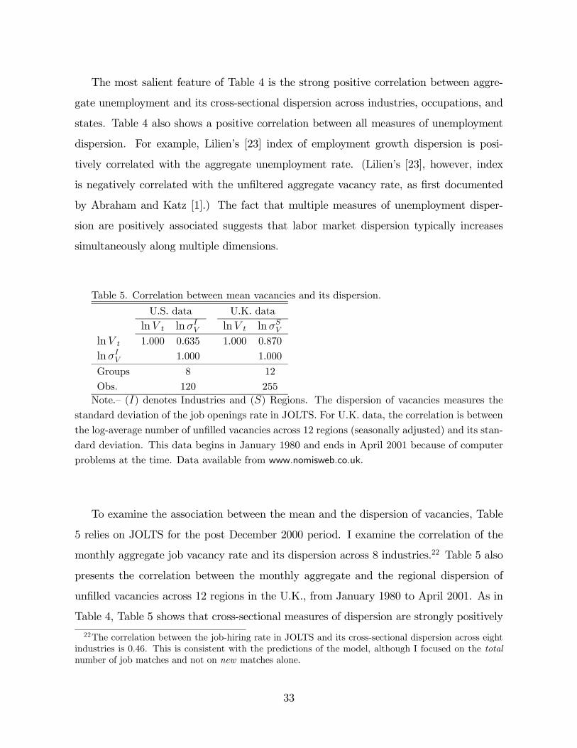
Table 5. Correlation between mean vacancies and its dispersion.

U.S. data U.K. data

ln ln ln lnln 1.000 0.635 1.000 0.870

ln 1.000 1.000

Groups 8 12

Obs. 120 255

Note.— () denotes Industries and () Regions. The dispersion of vacancies measures the

standard deviation of the job openings rate in JOLTS. For U.K. data, the correlation is between

the log-average number of unfilled vacancies across 12 regions (seasonally adjusted) and its stan-

dard deviation. This data begins in January 1980 and ends in April 2001 because of computer

problems at the time. Data available from www.nomisweb.co.uk.

To examine the association between the mean and the dispersion of vacancies, Table

5 relies on JOLTS for the post December 2000 period. I examine the correlation of the

monthly aggregate job vacancy rate and its dispersion across 8 industries.22 Table 5 also

presents the correlation between the monthly aggregate and the regional dispersion of

unfilled vacancies across 12 regions in the U.K., from January 1980 to April 2001. As in

Table 4, Table 5 shows that cross-sectional measures of dispersion are strongly positively

22The correlation between the job-hiring rate in JOLTS and its cross-sectional dispersion across eight

industries is 0.46. This is consistent with the predictions of the model, although I focused on the total

number of job matches and not on new matches alone.

33

correlated with aggregate vacancies. Moreover, in the U.S., the trend component of

vacancies, ln , is positively correlated with the trend component of ln , ln

, and

ln . (These estimates, available upon request, are not surprising given Tables 3 and 4.)

Overall, Tables 4 and 5 verify an important prediction of the model: both unemploy-

ment and vacancies covary positively with their cross-sectional dispersion. In the model,

changes in the structure of the economy are sectorally unbalanced (e.g., Proposition 4 and

Tables 1 and 2). In this fashion, the model rationalizes the positive correlation between

mean unemployment and vacancies, and their cross-sectional dispersion.23

5 Some elaborations of the model

Congestion. It is possible to incorporate congestion in the market assignment. As in

Lagos [21], assume that the technology for the basic model is Leontief, i.e., ( ) =

min[ ]. A motivation behind it is that the short-side of the market is served: if there

are () () jobs in , ()− () jobs will not “meet” workers; these jobs will remain

unused. The basic capital assignment problem is:

() ≡ max()

½Z 1

0

()min [() ()] :

Z 1

0

() ≤

¾. (24)

As in Lagos [21], assume that the market (not a social Planner) equalizes average

productivities: µ()min

∙1

()

∗()

¸−

¶∗() = 0. (25)

If () , then ∗() = 0, because these locations do not cover the cost of capital.

If () , then ()()∗() = . These assignments are directed toward markets

with higher values of ()(). Since () 1, these sub-markets will have an excess

supply of capital, i.e., ∗() (). If aggregate capital is small (in a sense made

23Changes in labor market dispersion are informative about changes in aggregate labor markets. In

an Appendix not for publication, I measure empirically the contribution of labor market dispersion to

movements along the short-run Beveridge curve, and to shifts in this curve. The analysis, based on

partial correlations, finds that the main contribution of dispersion measures is in explaining changes in

medium-run trends. Lilien’s [23] index, does not help explain the shifts in the aggregate Beveridge curve.

34

precise below), capital will be rationed creating an excess supply of workers:

Proposition 6 The market assignment (25) exhibits an excess supply of capital in sub-

markets with () , and an excess supply of workers in markets with () . If

min∈[01] () ≥ , workers are in excess supply if

Z 1

0

()().

In addition to demand uncertainty, captured by (), unemployment and vacancies in

this proposition are due to local shortages of capital and labor. In the Leontief case both

and are free parameters. Thus, an excess supply of workers has two possible causes:

either is too high or is too low, which is the only case Lagos ([21], Proposition 2)

discussed.

Unemployment in the previous market assignment is inefficient due to a coordination

problem. The optimal allocation is such that ∗() = () in () ≥ , given capital

availability; see, e.g., Akerlof [3]. In the market assignment (25), however, ∗() ()

in () ≥ . Agents do not take into account the marginal reduction in worker-job

meeting rates imposed as more capital is assigned to productive sub-markets. Thus, too

much capital is directed toward the most productive locations leaving workers in less

productive locations unemployed. In this case, redirecting capital to the least productive

locations will improve labor market conditions. Notice, however, that the excess supply

of capital and labor in Proposition 6 requires a Leontief technology. In a CES function,

( ) = [ + ]1, Proposition 6 applies if → −∞. If −∞, there will be noexcesses of workers and jobs.24

Rest unemployment. Other types of unemployment could be studied. Jovanovic

[20], Gouge and King [17], and Alvarez and Shimer [5] have examined rest unemployment,

in which workers have an “outside option” with a payoff 0. These authors consider

this modification because in its absence, search unemployment would vary positively with

improvements in productivity, as in specifications (1) and (2) in Tables 1 and 2.

24When −∞, there will be no excess supply of capital. If −∞ 0, (0 ) = 1. In this

case, the first order condition is [()(∗() ())− ] ∗() = 0. Thus, ∗() = 0 if ()1 .

Workers in these locations may be considered unemployed. This type of unemployment was studied by

Akerlof [3].

35

If workers value leisure or non-market activities such as rest, workers with potential

wages below will rest. Workers with potential wages above may still become unem-

ployed because resting and waiting are conceptually very different. The central difference

between search, rest, and waiting is the degree of separation from the labor market.

Searchers are in transition between labor markets. Individuals who rest are not in the

labor market (or marginally attached to it), so they will not work in the current period.

Workers who are waiting are in the labor market, and hence they are more likely to

find employment than the other two types of workers. The data seems to support this

prediction; see, e.g., Jones and Riddell [19].

Aggregate uncertainty. I focused on a stationary allocation without aggregate

uncertainty. In an Appendix not for publication I examine a general case that allows

the aggregate state to be uncertain. Following Miao [26], I establish the existence of

a solution in a much more general case. Uniqueness, however, cannot be established

in general. Numerical solutions, such as those described in Cooley ([13], chapter 4) for

models of heterogeneous agents, could be considered to incorporate aggregate shocks to

the quantitative analyses of the present model.

6 Conclusions

This paper constructed a general equilibrium model of mismatch. In the model, aggregate

demand is uncertain. Unemployment and vacancies arise due to the inability of market

participants to fully anticipate and respond to changes in demand. Workers with certain

qualifications or in specific locations are unemployed because there is no demand for the

commodities they produce. Workers cannot relocate or learn new skills instantaneously.

Movements to a different sub-market are possible but, as in Lucas and Prescott [24], these

movements take time and involve a period of (search) unemployment.

The model focused on the medium-run behavior of the labor market. In U.S. data,

the volatility of the medium-run components of unemployment and vacancies is as im-

portant as the volatility of business cycle components, and unemployment and vacancies

36

tend to covary positively in the medium run. These features of the data suggest changes

in the structure of the labor market that appear to shift the Beveridge curve. The the-

ory accounts for these shifts as a consequence of capital and labor reallocations. The

reallocation of capital and labor leads to a simultaneous increase in unemployment and

vacancies due to their complementarity in production. These changes are sectorally un-

balanced because demand uncertainty and productivity differ across sub-markets. Thus,

episodes of high unemployment or high vacancies are accompanied by high cross-sectional

dispersion. Mismatch increases in the sense of higher imbalances, e.g., higher dispersion in

unemployment and vacancies across labor markets, but also in the sense that the number

of unemployed workers and vacant jobs in different locations increases.

Although the model has many interesting theoretical and empirical implications, sev-

eral simplifying assumptions were made. Cyclical fluctuations in unemployment and va-

cancies appear to be as important as secular changes. The paper, however, focused entirely

on “steady state” comparisons. A natural next step would be to seek an integrated view of

the labor market. I also abstracted from risk considerations. The all-or-nothing structure

of production is a tractable assumption that yields simple predictions about higher mo-

ments of labor market outcomes not possible under more general assumptions. The model

also focused on perfectly competitive sub-markets and assumed away matching frictions

within each sub-market. The present framework, however, could be used for thinking

about labor market policies that interfere with the creation of jobs and the reallocation

of capital and labor.

References

[1] Abraham, K.G. and Katz, L.F. (1986) “Cyclical Unemployment: Sectoral Shifts or

Aggregate Disturbances?,” Journal of Political Economy, Vol. 94, 507-522.

[2] Abraham, K.G. (1987) “Help Wanted Advertising, Vacancies, and Unemployment,”

Brookings Papers on Economic Activity, Vol. 1, 207-248.

37

[3] Akerlof G. (1969) “Structural Unemployment in a Neoclassical Framework,” Journal

of Political Economy, Vol. 77, 399-407.

[4] Alvarez, F. and Veracierto, M. (1999) “Labor-Market Policies in an Equilibrium

Search Model,” NBER Macroeconomics Annual, Vol. 14, 265-304.

[5] Alvarez, F. and Shimer, R. (2011) “Search and Rest Unemployment,” Econometrica,

Vol. 79, 75-122.

[6] Bergin, J. and Bernhardt, D. (1992) “Anonymous Sequential Games with Aggregate

Uncertainty,” Journal of Mathematical Economics, Vol. 21, 543-562.

[7] Blanchard, O.J. and Diamond, P. (1989) “The Beveridge Curve,” Brookings Papers

on Economic Activity, Vol. 1, 1-76.

[8] Blanchflower, D.G. and Oswald, A.J. (1994) The Wage Curve, MIT Press.

[9] Bleakley, H. and Fuhrer, J.C. (1997) “Shifts in the Beveridge Curve, Job Matching,

and Labor Market Dynamics,” New England Economic Review, Vol. 28, 3-19.

[10] Butters, G.R. (1977) “Equilibrium Distributions of Sales and Advertising Prices,”

Review of Economic Studies, Vol. 44, 465-491.

[11] Bryant, J. (1980) “Competitive Equilibrium with Price Setting Firms and Stochastic

Demand,” International Economic Review, Vol. 21, 619-626.

[12] Carlton, D.W. (1978) “Market Behavior with Demand Uncertainty and Price Inflex-

ibility,” American Economic Review, Vol. 68, 571-587.

[13] Cooley T. (1995) Frontiers of Business Cycle Research, Princeton University

Press.

[14] Daly, M., Hobijn, B., and Valletta, R. (2011) “The Recent Evolution of the Nat-

ural Rate of Unemployment,” Working Paper 2011-05, Federal Reserve Bank of San

Francisco.

38

[15] Dana, J. (1999) “Equilibrium Price Dispersion Under Demand Uncertainty: The

Roles of Costly Capacity and Market Structure,” Rand Journal of Economics, Vol.

30, 632-660.

[16] Eden, B. (1990) “Marginal Cost Pricing When Spot Markets are Complete,” Journal

of Political Economy, Vol. 98, 1293-1306.

[17] Gouge, R. and King, I. (1997) “A Competitive Theory of Employment Dynamics,”

Review of Economic Studies, Vol. 64, 1-22.

[18] Jackman, R., Layard, R., and Savouri, S. (1991) “Mismatch: A Framework for

Thought [with comments by Sherwin Rosen],” in Schioppa, F.P. (Ed.) Mismatch

and Labour Mobility, Cambridge University Press.

[19] Jones, S.R.G. and Riddell, C. (1999) “The Measurement of Unemployment: An

Empirical Approach,” Econometrica, Vol. 67, 147-161.

[20] Jovanovic, B. (1987) “Work, Rest, and Search: Unemployment, Turnover, and the

Cycle,” Journal of Labor Economics, Vol. 5, 131-148.

[21] Lagos, R. (2000) “An Alternative Approach to Search Frictions,” Journal of Political

Economy, Vol. 108, 851-873.

[22] Landsburg, S.E. and Eden, B. (1987) “On the Competitive Resolution of Trading

Uncertainty,” Journal of Economic Theory, Vol. 47, 66-75.

[23] Lilien, D. M. (1982) “Sectoral Shifts and Cyclical Unemployment,” Journal of Polit-

ical Economy, Vol. 90, 777-793.

[24] Lucas, R.E. and Prescott, E.C. (1974) “Equilibrium Search and Unemployment,”

Journal of Economic Theory, Vol. 7, 188-209.

[25] Medoff, J.L. (1983) “U.S. Labor Markets: Imbalance, Wage Growth, and Productiv-

ity in the 1970s,” Brookings Papers on Economic Activity, Vol. 1, 87-128.

39

[26] Miao, J. (2006) “Competitive Equilibria of Economies with a Continuum of Con-

sumers and Aggregate Shocks,” Journal of Economic Theory, Vol. 128, 274-298.

[27] Mortensen, D.T. (2009) “Island Matching,” Journal of Economic Theory, Vol. 144,

2336-2353.

[28] Nickell, S. and Nunziata, L., Ochel, W., and Quintini, G. (2003) “The Beveridge

Curve, Unemployment and Wages in the OECD from the 1960s to the 1990s,” in

Aghion, P., Frydman, R., Stiglitz, J., and Woodford M. (eds.) Knowledge, In-

formation and Expectations in Modern Macroeconomics: in Honor of

Edmund S. Phelps, Princeton University Press.

[29] Peters, M. and Winters, R.A. (1983) “Market Equilibrium and the Resolution of

Uncertainty,” Canadian Journal of Economics, Vol. 16, 381-390.

[30] Petrongolo, B. and Pissarides, C. (2001) “Looking into the Black Box: A Survey of

the Matching Function,” Journal of Economic Literature, Vol. 39, 390-431.

[31] Pissarides, C. (2000) Equilibrium Unemployment Theory, Cambridge Mass.:

MIT Press.

[32] Prescott, E.C. (1975) “Efficiency of the Natural Rate,” Journal of Political Economy,

Vol. 83, 1229-1236.

[33] Schioppa, F.P. (1991) Mismatch and Labour Mobility, Cambridge University

Press.

[34] Shimer, R. (2007) “Mismatch,” American Economic Review, Vol. 97, 1074-1101.

[35] Stokey, N.L., Lucas Jr., R.E., and Prescott, E.C. (1989) Recursive Methods in

Economic Dynamics, Harvard University Press.

40

7 Appendix A

Aggregate variances. Expression (12) ignores covariance terms in the variance of

vacancies. In general,

[()] = E

"µZ 1

0

[( )− ()]

¶2#. (A1)

Upon expansion, (A1) yields

[()] = E∙Z 1

0

[( )− ()]2

+ 2

Z 1

0

Z 1

0

[( )− ()][(0 )− (

0)]0¸. (A2)

The first term in (A2) is the aggregate over individual variances in (12). The second

term depends on the covariance structure. To solve for this term, notice that under

Bernoulli random variables this covariance becomes [Pr( : ( )−()) = 1][Pr( :(

0 )− (0)) = 1]()(0). Thus,

[()] =

Z 1

0

[( )] + 2

Z 1

0

Z 1

0

(1− ())∗ ()2(1− (

0))∗ (0)20.

Since the covariance depends on quadratic terms for (1 − ()), which are likely to

be small, it is reasonable to use the approximation (12) in the text. Notice that the

approximation will be exact if the changes in demand across locations were independent.

The absence of aggregate uncertainty. In the dynamic model, I treat the ag-

gregate state ( ) as a deterministic object despite the presence of location-specific

productivity shocks. In here I show that the relevant state variables evolve deterministi-

cally.

Let the transition function for the shock () beΦ([ ] ()) ≡ Pr(0 : +1( 0) ∈[ ]|()), i.e., the probability of observing future productivity of location in the

interval [ ] given (). To be explicit about the role of idiosyncratic shocks, let (())

A1

be the labor force in location at the beginning of period . Let Ω represent the possible

states of nature. At the end of period , when searchers arrive, the mass of workers in

[ ] is

Z

+1(()). The distribution of the labor force at the beginning of +1, after

shocks are realized, is

+1([ ] 0) =

ZΩ

Z

+1(+1( 0))Φ(0 ()). (A3)

This distribution is a random measure as it depends on the location-specific shocks.

By assuming that individual shocks do not lead to aggregate uncertainty, in the sense

considered by Bergin and Bernhardt [6], I can treat the distribution of the labor force as

a deterministic state variable. For this assumption to hold, the distribution of individual

shocks across locations, for a given 0, should be the same as the distribution over states

Ω for any given location. This interpretation is in the spirit of the Law of Large Numbers

for the continuum; see, e.g., Bergin and Bernhardt [6]. In this case, +1([ ] 0) in (A3)

can be written as:

+1([ ]) =

Z 1

0

+1(())Φ([ ] ()), (A4)

which is deterministic.

Although is deterministic, it has no “nice” properties. For example, more than one

future distribution +1 may be consistent with the current distribution (i.e., +1 is

not a contraction mapping). This problem is typical of dynamic economies with frictions

and heterogeneous agents.

Proof of Proposition 1 (Uniqueness). The social planner solves

( ) ≡ max()()

Z 1

0

()()(() ())+

∙ −

Z 1

0

()

¸. (A5)

To see that there is no other feasible assignment of capital that brings higher value

note that concavity implies (() ())−(∗ () ()) ≤ (∗ () ())[()−∗ ()].

Assume that () is another feasible assignment of capital. From the first order condition

A2

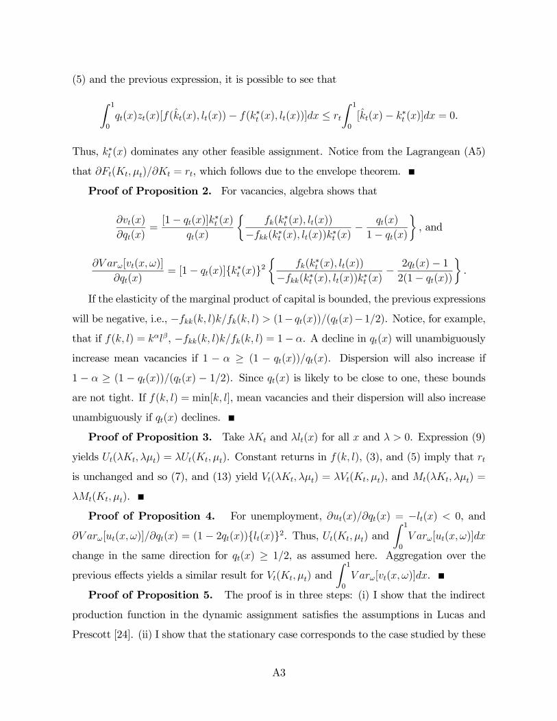
(5) and the previous expression, it is possible to see that

Z 1

0

()()[(() ())− (∗ () ())] ≤

Z 1

0

[()− ∗ ()] = 0.

Thus, ∗ () dominates any other feasible assignment. Notice from the Lagrangean (A5)

that ( ) = , which follows due to the envelope theorem.

Proof of Proposition 2. For vacancies, algebra shows that

()

()=[1− ()]

∗ ()

()

½(

∗ () ())

−(∗ () ())∗ ()− ()

1− ()

¾, and

[( )]

()= [1− ()]∗ ()2

½(

∗ () ())

−(∗ () ())∗ ()− 2()− 12(1− ())

¾.

If the elasticity of the marginal product of capital is bounded, the previous expressions

will be negative, i.e., −( )( ) (1− ())(()−12). Notice, for example,that if ( ) = , −( )( ) = 1− . A decline in () will unambiguously

increase mean vacancies if 1 − ≥ (1 − ())(). Dispersion will also increase if

1 − ≥ (1 − ())(() − 12). Since () is likely to be close to one, these boundsare not tight. If ( ) = min[ ], mean vacancies and their dispersion will also increase

unambiguously if () declines.

Proof of Proposition 3. Take and () for all and 0. Expression (9)

yields ( ) = ( ). Constant returns in ( ), (3), and (5) imply that

is unchanged and so (7), and (13) yield ( ) = ( ), and ( ) =

( ).

Proof of Proposition 4. For unemployment, ()() = −() 0, and

[( )]() = (1− 2())()2. Thus, ( ) and

Z 1

0

[( )]

change in the same direction for () ≥ 12, as assumed here. Aggregation over the

previous effects yields a similar result for ( ) and

Z 1

0

[( )].

Proof of Proposition 5. The proof is in three steps: (i) I show that the indirect

production function in the dynamic assignment satisfies the assumptions in Lucas and

Prescott [24]. (ii) I show that the stationary case corresponds to the case studied by these

A3

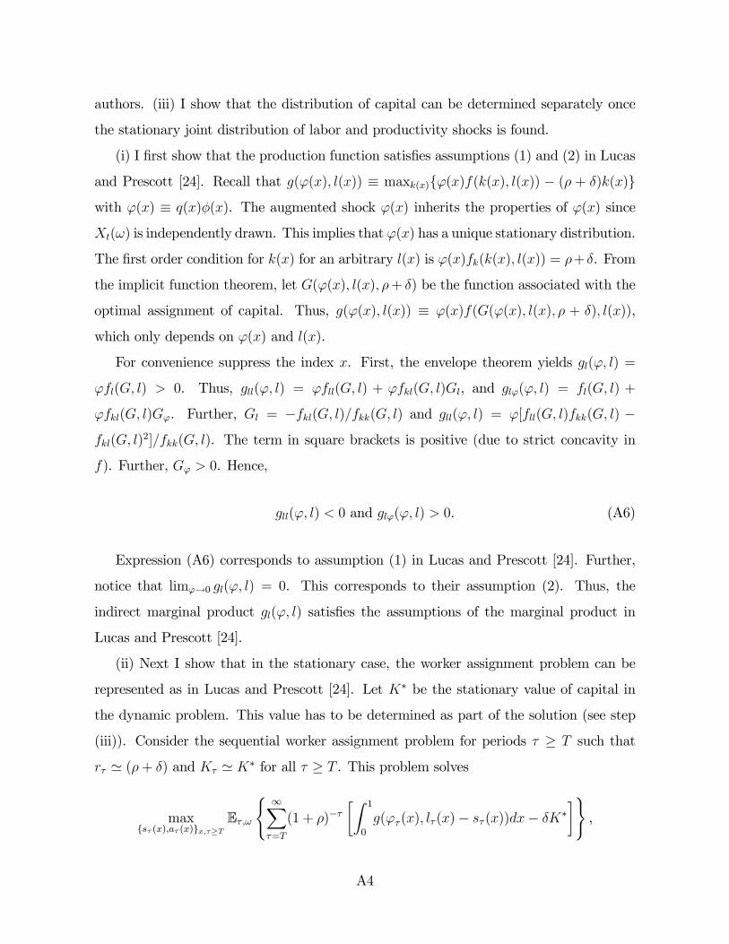
authors. (iii) I show that the distribution of capital can be determined separately once

the stationary joint distribution of labor and productivity shocks is found.

(i) I first show that the production function satisfies assumptions (1) and (2) in Lucas

and Prescott [24]. Recall that (() ()) ≡ max()()(() ()) − ( + )()with () ≡ ()(). The augmented shock () inherits the properties of () since

() is independently drawn. This implies that () has a unique stationary distribution.

The first order condition for () for an arbitrary () is ()(() ()) = + . From

the implicit function theorem, let (() () + ) be the function associated with the

optimal assignment of capital. Thus, (() ()) ≡ ()((() () + ) ()),

which only depends on () and ().

For convenience suppress the index . First, the envelope theorem yields ( ) =

( ) 0. Thus, ( ) = ( ) + ( ), and ( ) = ( ) +

( ). Further, = −( )( ) and ( ) = [( )( ) −( )

2]( ). The term in square brackets is positive (due to strict concavity in

). Further, 0. Hence,

( ) 0 and ( ) 0. (A6)

Expression (A6) corresponds to assumption (1) in Lucas and Prescott [24]. Further,

notice that lim→0 ( ) = 0. This corresponds to their assumption (2). Thus, the

indirect marginal product ( ) satisfies the assumptions of the marginal product in

Lucas and Prescott [24].

(ii) Next I show that in the stationary case, the worker assignment problem can be

represented as in Lucas and Prescott [24]. Let ∗ be the stationary value of capital in

the dynamic problem. This value has to be determined as part of the solution (see step

(iii)). Consider the sequential worker assignment problem for periods ≥ such that

' (+ ) and ' ∗ for all ≥ . This problem solves

max () ()≥

E

( ∞X=

(1 + )−∙Z 1

0

(() ()− ())− ∗¸),

A4

subject to (18) and (19). This problem is the analog of (15).

The previous problem can be studied using a “representative island” because the

Lagrange multiplier associated with the feasibility constraint (19) is independent of and

because the influence of the distribution of the labor force on has been suppressed. The

analysis of a representative island yields the same results as those in Lucas and Prescott

[24]. Their existence results and characterizations apply here.

(iii) The only aspect to be determined is the distribution of the capital assignments.

Suppose that the shocks and the labor force are distributed across locations according

to Ψ(() ()). Except for the case when the stationary allocation involves no worker

search, the process (() ()) has a unique stationary distribution Ψ∗; see Lucas and

Prescott ([24], Proposition 3) and Stokey, Lucas, and Prescott ([35], section 13.8).

Let ∗(() ()) be the optimal search decision given a state (() ()). Recall

that (() () + ) is the optimal capital assignment given () and (), and an

opportunity cost + . Then,

∗ =Z 1

0

(() ()− ∗(() ()) + )Ψ∗(),

which uniquely determines the aggregate capital stock, ∗.

Proof of Proposition 6. From the market assignment rule (25) it follows that

workers in locations () will be in excess supply. These workers do not cover the

opportunity cost of capital. In all other locations, () ≥ , (25) implies that ∗() (),

and so capital will be in excess supply. The total capital assigned is

Z 1

−1()∗() =

1

Z 1

−1()()(). (A7)

If min∈[01] () ≥ , then −1() → 0. If the right-hand-side of (A7) is larger than ,

capital will be rationed.

A5

8 Appendix B: Additional Results [NOT FOR PUB-

LICATION]

Measuring the importance of reallocational shocks. It is not possible to identify

the causes of changes in labor market dispersion as being a rise in demand uncertainty or

other (reallocational) shocks to the supply-side of the economy. Thus, the main objective

of the following exercise is not to causally explain unemployment movements, but rather

to see if the factors that influence labor market dispersion are quantitatively important

for understanding aggregate unemployment and vacancies.

For that purpose, consider a reduced-form Beveridge curve:

ln = ln + ln + , (B1)

where is the slope of the short-run Beveridge curve and ln is the medium-run com-

ponent, which must be estimated jointly with . I consider a third-order polynomial in

time represented by ln = 1 + 22 + 3

3. This specification provides a simple but

flexible method to estimate medium-run trends.25

Consider next an alternative reduced-form Beveridge curve:

ln = 0 ln + ln 0 + ln

+ 0, (B2)

where the dispersion of unemployment, ln , has been controlled for. Thus, (B2) es-

timates the short-run correlation between unemployment and vacancies as well as the

medium-run trend of unemployment after removing the influence of variables that affect

microeconomic dispersion. For example, if the variables that affect microeconomic dis-

persion bear no relationship with the variables that influence aggregate labor markets,

then 0 should be equal to . However, if aggregate unemployment, vacancies, and mi-

25Alternative specifications such as a linear trend are less flexible, but available upon request. (The

Hodrick-Prescott trend cannot be estimated jointly with .) Notice that (B1) examines the Beveridge

curve from the unemployment side. I examined similar estimates using vacancies as the dependent

variable and controlling for the dispersion of vacancies, ln . The sample in these estimates is limited,as JOLTS began in December, 2000. During that period, there were no mayor recessions.

B1

croeconomic labor market dispersion are jointly determined, then |0| || because partof the variation in vacancies and the medium-run trend will be captured by .

Table B1. Reduced-form Beveridge curve and the contribution of labor market dispersion.

Dependent variable: ln

A. End of sample, December, 2007.

(1) (2) (3) (4) (5) (6) (7) (8) (9) (10)

ln −0.37 −0.76 0.10 −0.28 −0.16 −0.47 −0.40 −0.62 −0.16 −0.76(0.04) (0.01) (0.01) (0.03) (0.01) (0.02) (0.01) (0.01) (0.04) (0.01)

ln |=1 0.86 0.24 0.31 0.46 0.86

0.00 0.00 0.00 0.00 0.00

R2 0.12 0.92 0.86 0.95 0.90 0.94 0.89 0.94 0.31 0.92

B. End of sample, December, 2010.

ln −0.46 −0.79 0.14 −0.24 −0.15 −0.40 −0.36 −0.59 −0.24 −0.78(0.03) (0.01) (0.01) (0.03) (0.01) (0.02) (0.01) (0.01) (0.04) (0.01)

ln |=1 1.02 0.22 0.30 0.48 1.01

0.00 0.00 0.00 0.00 0.00

R2 0.21 0.89 0.87 0.95 0.91 0.94 0.90 0.94 0.36 0.89

ln X X

ln X X

ln X X

ln X X

Note.— Robust standard errors in parentheses. ln |=1= 1+2+ 3. In curly brackets is the

p-value of an F-test on the significance of 123. All samples begin in January, 1976.

The logic of partial correlations and common dependence implies that ( − 0) es-

timates the contribution of variables that influence microeconomic dispersion to the move-

ments along the short-run Beveridge curve, whereas the ratio (ln |=1−ln 0|=1) ln |=1

estimates such contribution to the medium-run component. Table B1 presents the esti-

mates of (B1) and (B2). I report the value of the point estimates for the medium-run

trend at = 1, e.g., ln |=1. Their significance is assessed with a joint F-test whosep-values are reported in curly brackets. Despite slight differences in the estimates, the

conclusions that arise prior to the 2007-2009 recession are robust.

B2

Specification (1) yields a point estimate for of −0.37 and an R2 of 0.12. Specification(2) yields = −0.76 and the R2 is 0.92. These estimates show that vacancies accountonly for a small proportion of the variability of unemployment (in the R2 sense), and that

the correlation between unemployment and vacancies is stronger in the short run than in

the medium run. The most useful contrast in Table A1 is between (2) and specifications

(4), (6), and (8). Comparing (2) and (4) shows that factors affecting unemployment

dispersion across industries contribute 63 percent (= 1 − 028076) to the movementsalong the Beveridge curve and 72 percent (= 1 − 024086) to the medium-run trends.The point estimates in (6) yield lower contributions to movements along the curve, 47

percent, and to changes in the trend, 63 percent. The same contributions in (8) are 20

and 40 percent. The contribution of Lillien’s [23] index of dispersion in (10) is zero.

Overall, the cross-sectional dispersion of unemployment helps explain about half of

the movements along the short-run Beveridge curve and about 60 percent of the medium-

run changes in aggregate unemployment. Thus, Table B1 suggests that the factors that

influence microeconomic dispersion are likely to play a central role in the aggregate labor

market.

A competitive market representation of the dynamic assignment. Here I

sketch the equivalence between a competitive market allocation and the social Planner

allocation studied in the text. Prescott and Rios-Rull [3] have extended Arrow-Debreu

classical competitive analysis to economies with “islands” such as the one studied here.

The equivalence just mentioned is perhaps not surprising because worker search is

appropriately priced by . In a competitive market, which can be defined along the same

lines of the basic model, the representative household takes prices () asgiven and maximizes the present discounted value of expected aggregate consumption

with respect to () () +1(), subject to:

() ++1(

) ≤ (1 + (−1)− )(

−1) +Z 1

0

() [()− ()] +Π(),

(17) and (18) for all ≥ 0. Firms also take prices as given. Profits are a residual and

B3

given by Π(). Static capital assignments are analogous to the ones studied in the basic

model. Finally, market clearing in each period takes place as before. In addition, the total

number of searchers must equal the total number of arrivals, i.e., (19). The equivalence

between a competitive market and the (constrained) social Planner assignment can be

established along familiar lines: the Euler equations, static optimality conditions, and

feasibility conditions are the same in both approaches.

Details on the equivalence to Lucas-Prescott. Consider the dynamic assignment

problem for periods ≥ such that ' ( + ) and ' ∗ for all ≥ . This

problem solves

max () ()≥

E

( ∞X=

(1 + )−∙Z 1

0

(() ()− ())− ∗¸),

subject to (18) and (19).

To see the equivalence suppress the index . The functional equation for this problem

is: W( ) = max( − ) + (1 + )−1E[W(0 0)]], subject to (18) and (19).The first order conditions are: − ( − ∗) − (1 + )−1E[W(

0 0)]∗ = 0, (1 +)−1E[W(

0 0)] − ∗ = 0. They are analogous to cases (i)-(iii) studied in the text.

The envelope condition is W( ) = ( − ∗) + (1 + )−1E[W(0 0)]. Associated

with the previous first order and envelope conditions there is a functional equation for

W( ) which is

W( ) = max ( ) + min[ (1 + )−1E[W(0 0)]].

For instance, in case (i), W( ) = . In case (ii), W( ) = ( ) + (1 +

)−1E[W(0 0)]. In case (iii), W( ) = ( ) + . The recursive representation

above is that of Lucas and Prescott [24]. This functional equation has a unique solution

which is nondecreasing in and nonincreasing in , see, e.g., Lucas and Prescott ([24],

Proposition 1).

To obtain the stationary distribution of the labor force, let ∗+1( () ()) be the

B4

labor force at the end of the period when searchers arrive. This variable depends on the

augmented productivity shock and the initial population. Let I· represent the indica-tor function. Let Γ(·) be the transition function that describes the law of motion of thestate.26 Transitions from (() ()) are described by Γ(0() 0()|() ()) ≡ Pr( :+1( ) ≤ 0() ∗+1( () ()) ≤ 0()|() = () () = ()), which corre-sponds to Γ(0() 0()|() ()) = Φ([0 0()] ())I∗+1(() ())) ∈ [0 0()].The transition function defines an operator P on distribution functions: suppose that

the productivity shocks and the labor force are distributed across locations according

to Ψ(() ()). Then, the joint distribution of these variables in the next period

is P(Ψ(0() 0()) =Z 1

0

Γ(0() 0()|() ())Ψ(() ()). Except for the casewhen the stationary allocation involves no worker search, the process (() ()) has a

unique stationary distribution Ψ∗ which is the solution to P(Ψ∗) = Ψ∗ see, e.g., Lucas

and Prescott ([24], Proposition 3) and Stokey, Lucas, and Prescott ([35], section 13.8).

This shows that there is a unique stationary distribution of the labor force derived from

Ψ∗(() ()). That is, ∗([ ]) =Z

()Ψ∗().

An economy with aggregate productivity shocks. Here I examine the dynamic

assignment problem under aggregate productivity shocks. It is necessary to treat the

distribution of jobs as a state variable, see, e.g., Kubler and Schmedders [2] and Miao

[26]. The analysis differs from the deterministic case because uniqueness of stationary

solutions cannot be established. Thus, I study non-stationary solutions. The notation

here follows closely the main text.

Aggregate productivity shocks are defined on a countable space (ZZ). Let =

( −1) be a history in Z = Z × Z−1. The value of 0 is given. Aggregate shocks

are a Markov process with transition function, : Z × Z → [0 1]. The transition

function has the Feller property as defined by Stokey, Lucas, and Prescott ([35], chap.

12). Let P([0 1]B) be the set of probability measures on [0 1] and define S ≡ K × Z.26The transition Γ does not depend on the aggregate capital stock and the distribution of the labor

force . Otherwise, the transition of the state would have to incorporate their law of motion. Once these

(deterministic) variables are included, there is no general uniqueness result such as the one discussed here.

Existence can be established in more general cases such as in the case of aggregate productivity shocks.

This case is discussed immediately below in this Appendix.

B5

The state in this economy is the aggregate capital stock, the aggregate productivity

shock, and the distribution of the labor force across locations. The state is a pair ( )

that lies in S × P([0 1]). The capital assignment to is a function ( ) with

: [0 1]× S×P([0 1])→ R+. Similar notation defines the assignment of workers.

Given and (−1 −1), capital, consumption and aggregate production are fea-

sible if ( ) ++1(

)− (1− )(−1 −1) ≤ (

). The objective of

the problem is to maximize the present expected value of aggregate consumption subject

to the feasibility conditions in the text: (3), (17), (18), and (19).

Proposition 7 There exists a solution to the dynamic assignment problem with aggregate

productivity shocks.

Proof. The proof of existence is constructive and it describes the solution and its

properties in two steps. The first step conditions on a sequence of aggregate distribu-

tions because, unlike Lucas and Prescott [24], decisions in period depend on the

expectation of the distribution of the labor force in + 1. In the second step, I study

the consistency requirements of the assignment that make this conditioning valid. This

approach follows Bergin and Bernhardt [6] and Miao [26].

The first step has three parts: (i-a) I examine capital accumulation decisions, (i-b) I

examine search decisions, and (i-c) I derive the law of motion for the distribution of the

labor force.

(i-a) For a given and a history ∈ S, capital accumulation decisions satisfy thefollowing Euler equation:

+ =

ZS+1

+1(+1 +1)(

+1),

with : (SS)→ [0 1] as the transition function for = ( ). Capital accumulation

decisions are continuous and the transition function ( +1) has the Feller property.

Since I have conditioned the decisions on , the construction of the transition functionfor is standard, see Stokey, Lucas, and Prescott ([35], Theorem 9.13). The Feller

property follows from Stokey, Lucas, and Prescott ([35], Theorem 9.14).

B6

(i-b) Search decisions also satisfy a series of Euler equations as those in the text.

For a given and a history ∈ S, there exists a continuous worker assignment( ) (

)∈[01] that satisfies the following Euler equations:½(()

) + E0∙+1(+1(

0) +1 +1)

1 +

¸− (

)

¾(

) = 0,

and ½(

)− E0∙+1(+1(

0) +1 +1)

1 +

¸¾(

) = 0.

Expectations are given by:

E0 [(+1( 0) +1 +1)] ≡ZΩ

ZS+1

(+1( 0) +1 +1)(

+1)Φ( 0),

for an arbitrary function (+1( 0) +1 +1). These expectations are defined over

location-specific and aggregate shocks because the distribution of the labor force has been

conditioned upon. The interpretation of the previous Euler equations is similar to that

in the text.

(i-c) Let represent the sequence ( −1;0 0). Recall that is a functionfrom S × P([0 1]) to P([0 1]) and let P([0 1])S denote the set of such functions. LetP∞([0 1]) ≡ ×∞=1P([0 1])S. Notice that lies in P∞([0 1]). At the beginning of period+ 1, distribution of the labor force is:

+1([ ] ) =

ZΩ

Z

+1(+1( 0) )Φ(

0), (B3)

=

Z 1

0

+1( )Φ([ ] ),

where the second line follows by the no aggregate uncertainty condition described in

Bergin and Bernhardt [6]. Expression (B3) is deterministic conditional on a history .

This completes the derivation of the evolution of the state of the economy.

(ii) A solution of the dynamic assignment problem requires consistency between de-

cisions that conditioned on and the sequence of distributions from (B3). Since

B7

equation (B3) defines a mapping T : P∞([0 1]) → P∞([0 1]), a topological fixed point

∗ = T(∗) is a solution to the assignment problem.

The rest of the proof follows the arguments in the proof of Miao ([26], Theorem

1) and applies Brouwer-Schauder-Tychonoff Fixed-Point Theorem to T. One needs to

show that the domain of T is compact, that T maps P∞([0 1]) into itself, and that T

is continuous. Because ( ) acts as a typical aggregate production function, the

aggregate capital is uniformly bounded or there is amaximum sustainable stock of capital.

To see this, consider a policy in which consumptions are always zero. The condition that

lim→∞ ( ) + 1− 1 implies that there is a +∞ that uniformly bounds .

The space of aggregate shocks Z is also bounded and compact by assumption. This

makes bounded and compact. Because the space [0 1] is compact, P([0 1]) is also

compact, see, e.g., Aliprantis and Border ([1], Theorem 15.11). Finally, recall that is a function from P∞([0 1]). Endowed with the product (or pointwise convergence)

topology, P∞([0 1]) and the set ∞ × P∞([0 1]) are compact, see, e.g., Aliprantis andBorder ([1], Theorem 2.69).

Because feasibilty in worker search is such that searchers arrive before the end of the

period, T() lies in P∞([0 1]). That is, the mapping T returns a distribution function in

P∞([0 1]). Finally, T is continuous because the search decisions and job assignments are

continuous. This establishes the existence of a solution to this general problem.

References

[1] Aliprantis, C.D. and Border, K.C. (1999) Infinite Dimensional Analysis, Springer-

Verlag.

[2] Kubler, F. and Schmedders, K. (2002) “Recursive Equilibria in Economies with In-

complete Markets,” Macroeconomic Dynamics, Vol. 6, 284-306.

[3] Prescott, E.C. and Rios-Rull, J.-V. (1992) “Classical Competitive Analysis of

Economies with Islands,” Journal of Economic Theory, Vol. 57, 73-98.

B8