A competitive iterative procedure using a time-indexed

model for solving flexible job shop scheduling problems

Karin Thornblada,b,1, Ann-Brith Stromberga, Michael Patrikssona, TorgnyAlmgrenb

aMathematical Sciences, Chalmers University of Technology and University ofGothenburg, SE-421 96 Goteborg, Sweden

bGKN Aerospace Engine Systems, Dep. of Logistics Development, SE-461 81Trollhattan, Sweden

Abstract

We investigate the efficiency of a discretization procedure utilizing a time-

indexed mathematical optimization model for finding accurate solutions to flexible

job shop scheduling problems considering objectives comprising the makespan and

the tardiness of jobs, respectively. The time-indexed model is used to find solu-

tions to these problems by iteratively employing time steps of decreasing length.

The solutions and computation times are compared with results from a known

benchmark formulation and an alternative, slightly enhanced version of the same.

For the largest instances—considering both objectives—the proposed method finds

significantly better solutions than the other models within the same time frame,

although there is a large difference in the performance of the models depending

on which objective is considered. This implies that the evaluation of scheduling

algorithms must be performed with respect to an objective that is suitable for the

real application for which they are intended. The minimization of the makespan

is no such objective, although it is the most widely used objective in research.

We propose an objective incorporating tardiness. The iterative procedure for solv-

ing the time-indexed model outperforms the other models regarding the time to

find the best feasible solution. We conclude that our iterative procedure with the

time-indexed model is competitive with state-of-the-art mathematical optimiza-

tion models. Since the proposed procedure quickly finds solutions of good quality

to large instances, our findings imply that the new procedure is beneficially utilized

for scheduling real flexible job shops.

Keywords: Flexible job shop scheduling, Time-indexed formulation, Mixedinteger linear programming (MILP), Discretization procedure, Benchmark,Minimize makespan, Tardiness

1

1. Introduction

The job shop scheduling problem is defined as that to find the optimalsequences of a given set of jobs on a given set of machines. Each job consistsof a number of operations which must be processed in a given order; this ismodeled by so-called precedence constraints. Associated with each operationis a machine and a processing time. The flexible job shop problem (FJSP) isan extension of the job shop problem in which each operation may be sched-uled in more than one of the machines (Brucker and Knust, 2012, Chapter4).

The purpose of this article is to investigate the competitiveness of an it-erative discretization procedure utilizing a time-indexed mixed integer linearprogramming (MILP) model in finding accurate solutions to flexible job shopscheduling problems. The MILP models include both binary and continuousvariables, and all the relations between the variables in the objective andconstraints are linear; see Nemhauser and Wolsey (1988). Our iterative solu-tion procedure is compared with a benchmark model presented by Ozguvenet al. (2010), which yielded the best results in the evaluation by Demir andIsleyen (2013). In the comparison we have also included a similar alternativemodel developed during the work with this article.

2. Related Work

In Manne (1960), the problem of sequencing jobs with precedence con-straints on a single machine is studied. The jobs’ starting times are repre-sented by continuous variables, and the decision variables are defined as yjqequals 1, if job j precedes job q, and 0 otherwise. In the operations researchliterature, there are many examples of models for job shops and flexible jobshops employing this type of variables; see, e.g., Ozguven et al. (2010) andLow et al. (2006).

Email addresses: karin.thornblad@gknaerospace.com (Karin Thornblad ),anstr@chalmers.se (Ann-Brith Stromberg), mipat@chalmers.se (Michael Patriksson),torgny.almgren@gknaerospace.com (Torgny Almgren)

1Corresponding author, GKN Aerospace Engine Systems, Dep. of Logistics Develop-ment, 9510KT, SE-461 81 Trollhattan, Sweden. Tel. +46 520 29 22 66.

August 19, 2013

An alternative means to formulating a MILP model for the flexible jobshop problem is to utilize discrete time-indexed variables. The planningperiod is then divided into a number of time steps of equal length. Thedecision variables in the time-indexed model are valued 1 if the correspondingoperation is scheduled to start at the beginning of a specific time step in aspecific resource, and 0 otherwise. The resulting formulation results in verylarge models in terms of numbers of both variables and constraints, but ittypically yields better optimistic estimates of the optimal objective value(see Section 3.2) than other MILP formulations of scheduling problems; seevan den Akker et al. (2000). In Berghman (2012), a time-indexed formulationoutperformed three other MILP models for the problem of parallel machinescheduling when the objective was to minimize a total weighted sum of thecompletion times. We obtained a similar result for a special case of the FJSPin a real production cell with the objective to minimize a weighted sum ofthe completion times and the tardiness (Thornblad, 2011).

The objective that is the most often utilized for scheduling problems isthe minimization of the makespan (Jain and Meeran, 1999). Other commonobjectives are related to the jobs’ earliness/tardiness and completion times,and/or inventory holding costs associated with the jobs. Out of the 22 arti-cles listed by Demir and Isleyen (2013), which presents mathematical models(some of the models being non-linear) concerning the FJSP, 16 consideredthe objective of minimizing the makespan; only ten considered other objec-tives, whereof five involving due dates. See Section 4 for a discussion of themakespan objective and an objective including tardiness, and their respectivesuitability for real applications.

Besides MILP, there are many methods devoted to finding good feasiblesolutions to scheduling problems. Constraint programming (CP) is an exactmethod which seems to yield good results, see, e.g., Sadykov and Wolsey(2006) for an evaluation of MILP and CP models for solving a multimachineassignment scheduling problem. There are many metaheuristics proposedfor flexible job shop scheduling problems, such as simulated annealing, tabusearch, and genetic algorithms amongst others, and combinations of these;see, e.g., Wang et al. (2012), Al-Hinai and ElMekkawy (2011), and Bayka-soglu and Ozbakir (2010). In Section 6, we compare the makespan foundby our models with those found by Behnke and Geiger (2012) and Bagheriet al. (2010), who employ CP and an artificial immune algorithm (AIA),respectively.

3

3. Mathematical formulations

3.1. Indices, sets, and parameters

The notation used throughout this article is as follows:

SetsJ the set of jobs; j ∈ J := {1, . . . , n}Nj the set of operations; i ∈ Nj := {1, . . . , nj}K the set of resources; k ∈ K := {1, . . . ,m}Mij the set of resources allowed for operation i of job j (Mij ⊆ K)T the set of time steps; u ∈ T := {0, . . . , T}

Parameterspijk the processing time of operation i of job j in resource krij the release date of operation i of job j, i.e., its earliest possible

starting timeδij the shortest possible remaining time from the starting time of

operation i of job j to the completion of job j` the length of the time steps in the time-indexed modelM a big number, at least as large as the makespan of the solution

to be computed

In all test instances considered in this article, the parts to be processedare assumed to be present in the job shop at the beginning of time step 0, i.e.,the job release dates are r1j = 0. Due to the precedence relations between theoperations within a job, no operation may be scheduled before the completionof the previous operation. Therefore, and since the processing time is resourcedependent, the release dates are defined as rij := ri−1,j+mink∈Mi−1,j

{pi−1,j,k},for i = 2, . . . , nj, j ∈ J . Similarly, the shortest possible remaining time fromthe start of operation i to the completion of job j is defined as δij := δi+1,j +mink∈Mij

{pijk}, for i = nj − 1, . . . , 1, j ∈ J , and δnjj := mink∈Mnjj{pnjjk}.

3.2. Time-indexed model

The planning horizon is divided into T intervals (i.e., time steps), each oflength ` > 0. The value of the parameter T has to be large enough such thatan optimal schedule is contained within the time horizon [0, T `]. Our time-indexed model is expressed in terms of the variables xijku, which are valued 1if operation i of job j is scheduled to start processing in resource k at the startof time interval u, and 0 otherwise. Throughout the article, for any z ∈ R we

4

define (z)+ := max{z, 0}. We first consider the objective of minimizing themakespan of the schedule, represented by the variable Cmax ∈ R; in Section 4we present an alternative objective based on the total (weighted) tardiness.The model is thus to

minimize Cmax (1a)

subject to∑k∈Mij

∑u∈T

xijku = 1, i ∈ Nj, j ∈ J , (1b)

∑k∈K\Mij

∑u∈T

xijku = 0, i ∈ Nj, j ∈ J , (1c)

∑j∈J

∑i∈Nj

u∑µ=(u−pijk+1)+

xijkµ ≤ 1, k ∈ K, u ∈ T , (1d)

∑k∈Mij

u−pijk∑µ=rij

xijkµ−∑

l∈Mi+1,j

u∑ν=ri+1,j

xi+1,jlν ≥ 0, u=ri+1,j, . . . , T−δi+1,j, (1e)

i = 1, . . . , nj−1, j∈J ,∑k∈Mnjj

∑u∈T

(u+ pnjjk)xnjjku ≤ Cmax, j ∈ J , (1f)

xijku = 0, u ∈ T \ {rij, . . . , T−δij}, (1g)

k ∈Mij, i ∈ Nj, j ∈ J ,

xijku ∈ {0,1}, i ∈ Nj, j ∈ J , k ∈ K, (1h)

u ∈ T .

The constraints (1b) ensure that each operation i of job j is scheduled tobe processed exactly once in an allowed resource. The constraints (1c) setall variables corresponding to an operation to zero for the set of resourcesin which the operation is not allowed to be processed; these constraints areredundant, but they are included since we discovered that the solver (AMPL-CPLEX12 (Fourer et al., 2002; IBM Corp., 2009)) was able to parallelize thecomputations such that they run faster (w.r.t. clocktime) when these con-straints were included. The constraints (1d) ensure that at most one opera-tion at a time is scheduled in each resource. The precedence constraints (1e)make sure that no operation starts processing before the preceding operationof the same job is completed. The makespan of the schedule is determined by

5

the constraints (1f). The constraints (1g) ensure that operation i of job j isscheduled neither before its release date nor such that it (or any succeedingoperations) would not be completed by the end of the planning horizon, i.e.,at time the T`; these constraints are redundant if all the jobs are ready to beprocessed at the time 0, but their inclusion reduces the number of variablesin the model. The model (1) will henceforth be referred to as TI-Cmax.

The number of precedence constraints (1e) is in the order of the totalnumber of operations times the total number of time steps. If an instanceof the model is too large, such that the time to solve its linear programming(LP) relaxation2 is too long for practical purposes, then an alternative setof precedence constraints may be used (its number being in the order of thetotal number of operations):

∑k∈Mij

T−δij∑µ=rij

(µ+ pijk)xijkµ ≤∑

l∈Mi+1,j

T−δi+1,j∑ν=ri+1,j

νxi+1,jlν , i=1,. . .,nj−1, j ∈ J . (2)

The LP relaxation of TI-Cmax is a model with the same variables, ob-jective, and constraints, except for the integrality constraints (1h), which aresubstituted by 0 ≤ xijku ≤ 1. The optimal objective value of the LP relax-ation of a model is called its LP bound, being a lower bound on the optimalobjective value of the original model including integrality constraints. Pro-vided that the integrality constraints (1h) are fulfilled, the constraints (2)are equivalent to (1e); they do, however, not yield as tight LP bounds asdo the constraints (1e). The model (1a)–(1d), (2), (1f)–(1h) will henceforthbe referred to as TI-prec-Cmax. In Section 3.3 we present the results forone test instance regarding the differences in the LP bounds of the modelsTI-Cmax and TI-prec-Cmax.

3.3. An alternative model

We next present an alternative model that we have developed, employingthe same type of variables as the benchmark model proposed by Ozguvenet al. (2010). Our model contains fewer variables and constraints than the

2The LP relaxation of a MILP model is a model comprising the same variables, objec-tive, and constraints except for the integrality constraints which are substituted by therespective lower and upper bounds of the integer variables; see (Nemhauser and Wolsey,1988, Chapter II.3, Section 1).

6

benchmark model, since the variables representing the completion times ofoperations and jobs employed in the latter model are redundant. The vari-ables used in our alternative model are

zijk =

{1, if operation i of job j is processed on resource k,

0, otherwise,

yijpqk =

1, if operation i of job j precedes operation p of job q in

resource k,

0, otherwise,

tijk = the starting time of operation i of job j in resource k, and

Cmax = the completion time for the last job (makespan).

Our alternative model, Alt-Cmax, is then formulated as that to

minimize Cmax, (3a)

subject to∑k∈Mij

zijk = 1, i ∈ Nj, j ∈ J , (3b)

tijk −Mzijk ≤ 0, k ∈Mij, i ∈ Nj, j ∈ J , (3c)

tpqk + ppqkzpqk − tijk −Myijpqk ≤ 0, k ∈Mij ∩Mpq, i ∈ Nj, (3d)

p ∈ Nq, j, q ∈ J , j < q,

tijk + pijkzijk − tpqk −M(1− yijpqk) ≤ 0, k ∈Mij ∩Mpq, i ∈ Nj, (3e)

p ∈ Nq, j, q ∈ J , j < q,∑k∈Mij

(tijk + pijkzijk)−∑

k∈Mi+1,j

ti+1,jk ≤ 0, i = 1, . . . , nj − 1, j ∈ J , (3f)

∑k∈Mnjj

(tnjjk + pnjjkznjjk

)≤ Cmax, j ∈ J , (3g)

tijk ≥ 0, k ∈Mij, i ∈ Nj, j ∈ J , (3h)

zijk ∈ {0,1}, k ∈Mij, i ∈ Nj, j ∈ J , (3i)

yijpqk ∈ {0,1}, k ∈Mij ∩Mpq, i ∈ Nj, (3j)

p ∈ Nq, j, q ∈ J , j < q.

7

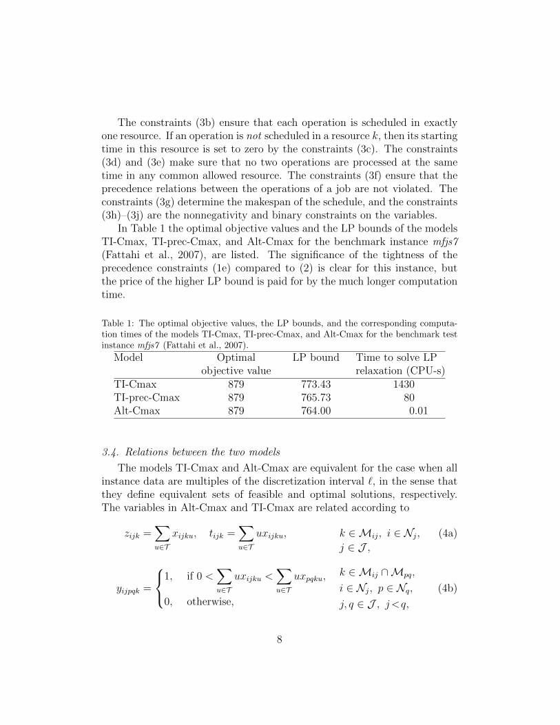
The constraints (3b) ensure that each operation is scheduled in exactlyone resource. If an operation is not scheduled in a resource k, then its startingtime in this resource is set to zero by the constraints (3c). The constraints(3d) and (3e) make sure that no two operations are processed at the sametime in any common allowed resource. The constraints (3f) ensure that theprecedence relations between the operations of a job are not violated. Theconstraints (3g) determine the makespan of the schedule, and the constraints(3h)–(3j) are the nonnegativity and binary constraints on the variables.

In Table 1 the optimal objective values and the LP bounds of the modelsTI-Cmax, TI-prec-Cmax, and Alt-Cmax for the benchmark instance mfjs7(Fattahi et al., 2007), are listed. The significance of the tightness of theprecedence constraints (1e) compared to (2) is clear for this instance, butthe price of the higher LP bound is paid for by the much longer computationtime.

Table 1: The optimal objective values, the LP bounds, and the corresponding computa-tion times of the models TI-Cmax, TI-prec-Cmax, and Alt-Cmax for the benchmark testinstance mfjs7 (Fattahi et al., 2007).

Model Optimal LP bound Time to solve LPobjective value relaxation (CPU-s)

TI-Cmax 879 773.43 1430TI-prec-Cmax 879 765.73 80Alt-Cmax 879 764.00 0.01

3.4. Relations between the two models

The models TI-Cmax and Alt-Cmax are equivalent for the case when allinstance data are multiples of the discretization interval `, in the sense thatthey define equivalent sets of feasible and optimal solutions, respectively.The variables in Alt-Cmax and TI-Cmax are related according to

zijk =∑u∈T

xijku, tijk =∑u∈T

uxijku, k ∈Mij, i ∈ Nj, (4a)

j ∈ J ,

yijpqk =

1, if 0 <∑u∈T

uxijku <∑u∈T

uxpqku,

0, otherwise,

k ∈Mij ∩Mpq,

i ∈ Nj, p ∈ Nq,j, q ∈ J , j <q,

(4b)

8

xijku =

{zijk, if u = tijk,

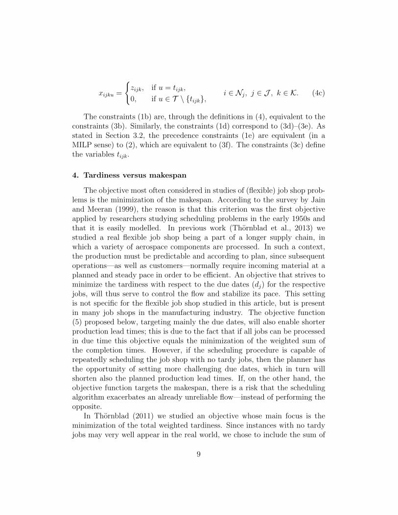
0, if u ∈ T \ {tijk},i ∈ Nj, j ∈ J , k ∈ K. (4c)

The constraints (1b) are, through the definitions in (4), equivalent to theconstraints (3b). Similarly, the constraints (1d) correspond to (3d)–(3e). Asstated in Section 3.2, the precedence constraints (1e) are equivalent (in aMILP sense) to (2), which are equivalent to (3f). The constraints (3c) definethe variables tijk.

4. Tardiness versus makespan

The objective most often considered in studies of (flexible) job shop prob-lems is the minimization of the makespan. According to the survey by Jainand Meeran (1999), the reason is that this criterion was the first objectiveapplied by researchers studying scheduling problems in the early 1950s andthat it is easily modelled. In previous work (Thornblad et al., 2013) westudied a real flexible job shop being a part of a longer supply chain, inwhich a variety of aerospace components are processed. In such a context,the production must be predictable and according to plan, since subsequentoperations—as well as customers—normally require incoming material at aplanned and steady pace in order to be efficient. An objective that strives tominimize the tardiness with respect to the due dates (dj) for the respectivejobs, will thus serve to control the flow and stabilize its pace. This settingis not specific for the flexible job shop studied in this article, but is presentin many job shops in the manufacturing industry. The objective function(5) proposed below, targeting mainly the due dates, will also enable shorterproduction lead times; this is due to the fact that if all jobs can be processedin due time this objective equals the minimization of the weighted sum ofthe completion times. However, if the scheduling procedure is capable ofrepeatedly scheduling the job shop with no tardy jobs, then the planner hasthe opportunity of setting more challenging due dates, which in turn willshorten also the planned production lead times. If, on the other hand, theobjective function targets the makespan, there is a risk that the schedulingalgorithm exacerbates an already unreliable flow—instead of performing theopposite.

In Thornblad (2011) we studied an objective whose main focus is theminimization of the total weighted tardiness. Since instances with no tardyjobs may very well appear in the real world, we chose to include the sum of

9

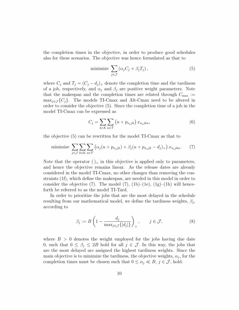
the completion times in the objective, in order to produce good schedulesalso for these scenarios. The objective was hence formulated as that to

minimize∑j∈J

(αjCj + βjTj) , (5)

where Cj and Tj = (Cj − dj)+ denote the completion time and the tardinessof a job, respectively, and αj and βj are positive weight parameters. Notethat the makespan and the completion times are related through Cmax :=maxj∈J {Cj}. The models TI-Cmax and Alt-Cmax need to be altered inorder to consider the objective (5). Since the completion time of a job in themodel TI-Cmax can be expressed as

Cj =∑k∈K

∑u∈T

(u+ pnjjk

)xnjjku, (6)

the objective (5) can be rewritten for the model TI-Cmax as that to

minimize∑j∈J

∑k∈K

∑u∈T

(αj(u+ pnjjk) + βj(u+ pnjjk − dj)+

)xnjjku. (7)

Note that the operator ( )+ in this objective is applied only to parameters,and hence the objective remains linear. As the release dates are alreadyconsidered in the model TI-Cmax, no other changes than removing the con-straints (1f), which define the makespan, are needed in this model in order toconsider the objective (7). The model (7), (1b)–(1e), (1g)–(1h) will hence-forth be referred to as the model TI-Tard.

In order to prioritize the jobs that are the most delayed in the scheduleresulting from our mathematical model, we define the tardiness weights, βj,according to

βj := B

(1− dj

maxj∈J {|dj|}

)+

, j ∈ J , (8)

where B > 0 denotes the weight employed for the jobs having due date0, such that 0 ≤ βj ≤ 2B hold for all j ∈ J . In this way, the jobs thatare the most delayed are assigned the highest tardiness weights. Since themain objective is to minimize the tardiness, the objective weights, αj, for thecompletion times must be chosen such that 0 ≤ αj � B, j ∈ J , hold.

10

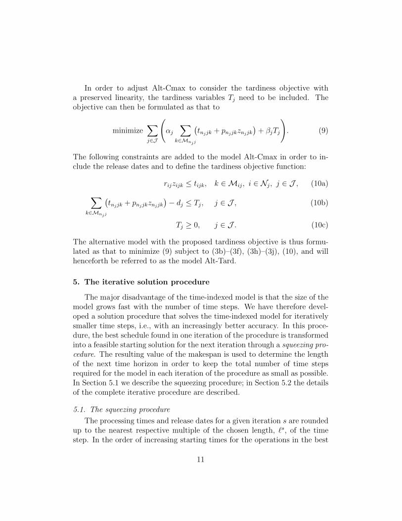
In order to adjust Alt-Cmax to consider the tardiness objective witha preserved linearity, the tardiness variables Tj need to be included. Theobjective can then be formulated as that to

minimize∑j∈J

(αj

∑k∈Mnjj

(tnjjk + pnjjkznjjk

)+ βjTj

). (9)

The following constraints are added to the model Alt-Cmax in order to in-clude the release dates and to define the tardiness objective function:

rijzijk ≤ tijk, k ∈Mij, i ∈ Nj, j ∈ J , (10a)∑k∈Mnjj

(tnjjk + pnjjkznjjk

)− dj ≤ Tj, j ∈ J , (10b)

Tj ≥ 0, j ∈ J . (10c)

The alternative model with the proposed tardiness objective is thus formu-lated as that to minimize (9) subject to (3b)–(3f), (3h)–(3j), (10), and willhenceforth be referred to as the model Alt-Tard.

5. The iterative solution procedure

The major disadvantage of the time-indexed model is that the size of themodel grows fast with the number of time steps. We have therefore devel-oped a solution procedure that solves the time-indexed model for iterativelysmaller time steps, i.e., with an increasingly better accuracy. In this proce-dure, the best schedule found in one iteration of the procedure is transformedinto a feasible starting solution for the next iteration through a squeezing pro-cedure. The resulting value of the makespan is used to determine the lengthof the next time horizon in order to keep the total number of time stepsrequired for the model in each iteration of the procedure as small as possible.In Section 5.1 we describe the squeezing procedure; in Section 5.2 the detailsof the complete iterative procedure are described.

5.1. The squeezing procedure

The processing times and release dates for a given iteration s are roundedup to the nearest respective multiple of the chosen length, `s, of the timestep. In the order of increasing starting times for the operations in the best

11

solution obtained in the previous iteration, the starting time of each operationis recalculated such that it is scheduled (on the same resource) as early aspossible, without violating any precedence or release date constraints. In theexample illustrated in Figure 1, the completion time of operation i of job jconstrains the starting time of operation p of job q, when the time steps arelarge; for the shorter time steps, the squeezing procedure schedules the startof operation p of job q at its release date, rpq.

Figure 1: The output of the time-indexed model from one iteration is squeezed into afeasible solution for the next iteration possessing shorter time steps.

Since the squeezing procedure retains the ordering of the operations oneach resource, and all precedence and release dates’ constraints are consid-ered by the squeezing procedure, the resulting schedule represents a feasiblesolution to the scheduling problem defined with the shorter time steps. Themakespan of the schedule obtained by the squeezing procedure applied to thesolution from the previous iteration is used as the time horizon, T s, for thenext iteration, for the case when the objective is to minimize the makespan.When minimizing the tardiness objective (7), the value assigned to the nexttime horizon equals the sum of the largest operation processing time and themakespan obtained by the squeezing procedure, since a smaller value of theobjective function in (7) may correspond to a larger makespan.

5.2. The iterative procedure

The iterative procedure employed for solving a time-indexed model isdescribed in Algorithm 1.

For each iteration s of the procedure, suitable values are assigned to thelength `s of the time steps and the time horizon T s. In order to determinea value for `1, the total number, V , of variables required for the smallestvalue of the time step, denoted ˜ to use in the last iteration is estimatedas V :=

(∑j∈J

∑i∈Nj

pij)(∑

j∈J nj), where pij := |Mij|−1

∑k∈Mij

pijk for

12

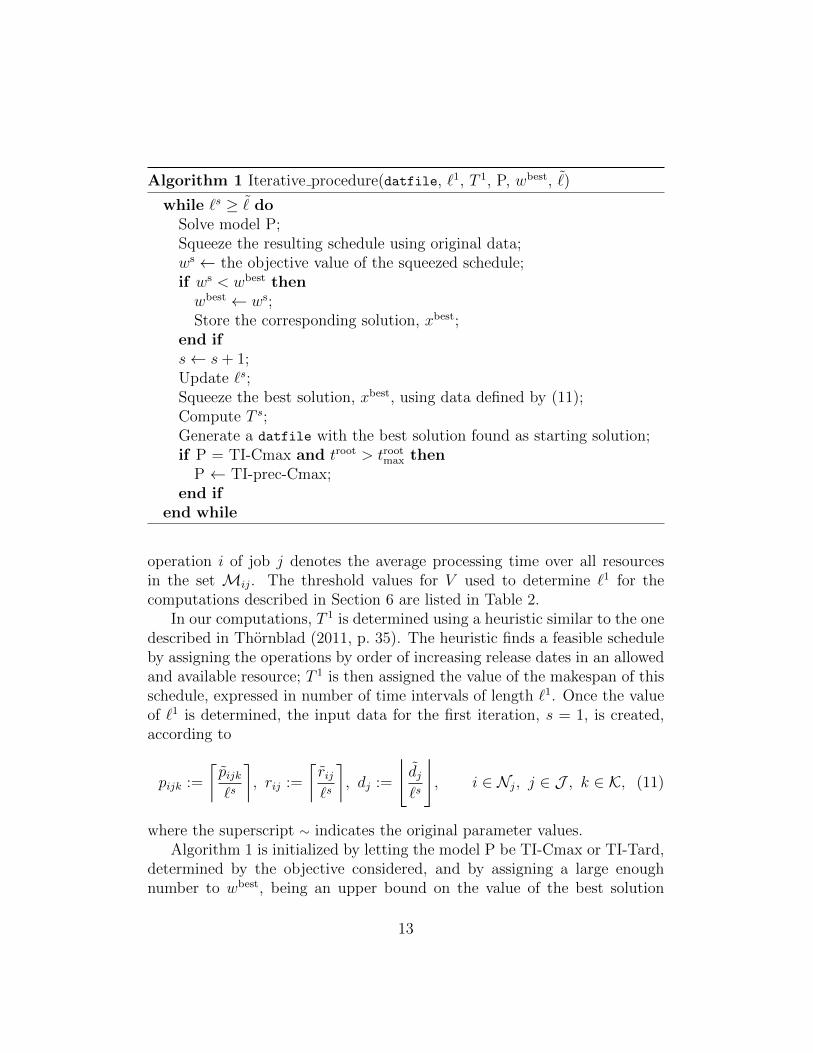
Algorithm 1 Iterative procedure(datfile, `1, T 1, P, wbest, ˜)

while `s ≥ ˜doSolve model P;Squeeze the resulting schedule using original data;ws ← the objective value of the squeezed schedule;if ws < wbest thenwbest ← ws;Store the corresponding solution, xbest;

end ifs← s+ 1;Update `s;Squeeze the best solution, xbest, using data defined by (11);Compute T s;Generate a datfile with the best solution found as starting solution;if P = TI-Cmax and troot > trootmax then

P ← TI-prec-Cmax;end if

end while

operation i of job j denotes the average processing time over all resourcesin the set Mij. The threshold values for V used to determine `1 for thecomputations described in Section 6 are listed in Table 2.

In our computations, T 1 is determined using a heuristic similar to the onedescribed in Thornblad (2011, p. 35). The heuristic finds a feasible scheduleby assigning the operations by order of increasing release dates in an allowedand available resource; T 1 is then assigned the value of the makespan of thisschedule, expressed in number of time intervals of length `1. Once the valueof `1 is determined, the input data for the first iteration, s = 1, is created,according to

pijk :=

⌈pijk`s

⌉, rij :=

⌈rij`s

⌉, dj :=

⌊dj`s

⌋, i ∈ Nj, j ∈ J , k ∈ K, (11)

where the superscript ∼ indicates the original parameter values.Algorithm 1 is initialized by letting the model P be TI-Cmax or TI-Tard,

determined by the objective considered, and by assigning a large enoughnumber to wbest, being an upper bound on the value of the best solution

13

Table 2: The threshold values of V used to determine `1 (the time step for the firstiteration). V is the estimated total number of variables required for the smallest desiredlength of the time step. The median of the processing times (in multiples of ˜) is denotedby p.

V ∈ `1

(∗1000)

(0, 10) 1[10, 50) p/8[50, 100) p/4[100, 500) p/2[500,∞) p

found so far. The input data required to solve the model P is denoteddatfile in the algorithm.

When considering the minimization of the makespan, the algorithm isterminated after either (i) the nth (with n = 3) feasible solution is found(cplex option solutionlim = n [see (IBM Corp., 2009, Chapter 7)]), or (ii) themipgap3 is less than a pre-specified number, or (iii) a pre-specified time limitis exceeded. If the computations were stopped due to the condition (i), then`s := `s−1, otherwise, `s := round(`s−1/ζ), where ζ > 1. In the computationswe employed ζ = 1.8. [Choosing ζ = 2 may result in an unfavourable datapattern in the rounding of parameters in (11).] Further, in order to reducethe total number of iterations, we set `s := ˜ = 1 when `s−1/ζ < 5. Thereason for this is that we found in the tests that the best solution is mostoften obtained for larger values of `s, and the last iteration, with `s = 1,is most often used to verify the optimality of a solution already found (orcompute a mipgap) rather than to find better feasible solutions.

The value T s of the time horizon is updated in the iterative procedure asdescribed in Section 5.1. For some of the largest instances of TI-Cmax, theCPU time, troot, required to solve the root relaxation (which is essentially theLP relaxation) exceeded the time limit. Therefore, the model TI-prec-Cmaxwas chosen instead of TI-Cmax if the value of troot exceeded a thresholdvalue, trootmax, in the previous iteration. In our computational testing, trootmax := 1

3The mipgap is defined as the relative difference between the best lower bound LB andthe best objective value z found. The definition used by CPLEX version 12 is mipgap :=|z−LB|

10−10+|z| · 100%.

14

CPU-second. For the model TI-Tard, the precedence constraints (1e) wereemployed in all iterations since they yielded smaller mipgap and shorter com-putation times.

6. Computational results

As mentioned in Section 3.3, we have chosen to compare the models bysolving the twelve largest benchmark test instances in Fattahi et al. (2007).We omitted the eight smallest instances out of the original 20, since theycan be computed in just a few seconds and are thus not that interesting forcomparison. All these test instances are available via Behnke and Geiger(2012), along with other instances for the flexible job shop problem. Thechosen instances range from n = 3, m = 3, and nj ≤ 3, for the smallestinstance sfjs9 to n = 12, m = 8, and nj ≤ 4, for the largest instance mfjs10.

The models compared are the time-indexed models TI-Cmax (TI-prec-Cmax) and TI-Tard (implemented through Algorithm 1), the alternativemodel (Alt-Cmax and Alt-Tard), and a benchmark model4 (BM-Cmax) de-veloped by Ozguven et al. (2010). The latter model is closely related to thealternative model; see Section 3.3. BM-Cmax was chosen to be our bench-mark model since it yielded the best results in the evaluation by Demir andIsleyen (2013). We also employed the benchmark model considering the tar-diness objective (9), implemented through the constraints (10a)–(10c). Thismodel is referred to as BM-Tard.

The computations were carried out using AMPL-CPLEX 12.1.0 (Foureret al., 2002; IBM Corp., 2009) on a computer with two 2.66 GHz Intel XeonX5650 processors, each with six cores (24 threads), with a total memory of48 Gbyte of RAM. The time limit for each call to the CPLEX solver fromthe iterative procedure was set to 7200 CPU-seconds. Since the iterativeprocedure calls the solver once each iteration, the total computation timemay exceed 7200 CPU-seconds.

4We implemented the benchmark model as it is formulated in Ozguven et al. (2010),except for a possible typo: In the precedence constraints regarding the operations ofthe same job, the sum over the completion times for operation i − 1 should, using ournotation, be over k ∈ Mi−1,j ; this is unclear in Ozguven et al. (2010, constraints (6), p.

1542). This mistake is also present in Demir and Isleyen (2013), where the benchmarkmodel is presented. In ibid., the constraints corresponding to (3d)–(3e) are defined forj ≤ q rather than for j < q. This is not incorrect, but the redundancy implies longercomputation times (Demir and Isleyen, 2013, constraints (2.5)-(2.6), p. 981)).

15

The squeezing procedure and the generation of input data files in eachiteration were implemented in MATLAB (2011). The total running time forthis Matlab program was around 15 seconds. Since the running time wouldonly be a fraction of a second if this code was optimized and implementedin, for example, C, the total running time of the iterative procedure wascalculated as the sum of the computation times used by CPLEX over all theiterations of Algorithm 1.

Since it is only in the last iteration (with `s = 1) that a lower bound on theoptimal objective value sought is guaranteed, and the mipgap is comparablewith that of the other models, the iterative procedure was run until the lastiteration was terminated due to either the computation time exceeding thetime limit of 7200 seconds, or that the mipgap in the last iteration (with`s = ˜ = 1) being less than 0.0005. This is due to the fact that the optimalobjective value—and the lower bound—in earlier iterations are expressed inmultiples of `s, and the lower bound can not be transformed into a lowerbound valid for the last iteration employing ˜. In order to ensure a faircomparison between the models, for each of the instances the time limitsfor solving BM-Cmax and Alt-Cmax (BM-Tard and Alt-Tard) were set tothe total CPU time needed by the iterative procedure implemented with themodel TI-Cmax (TI-Tard).

6.1. Test results for the minimization of the makespan

In Table 3, we present the results from employing the iterative procedurewith TI-Cmax are compared with the results from solving BM-Cmax andAlt-Cmax for the seven largest instances mfjs4-10. All the smaller instances,namely sfjs9-10, and mfjs1-3, were solved to optimality within 20 CPU-seconds by all the three models.

The time limit was reached before the iterative procedure with TI-Cmaxhad established optimality for the instances mfjs4 and mfjs6, although thetime to find the best feasible solution (”time to best”) is competitive withthe models BM-Cmax and Alt-Cmax;, see Figure 2. The computation timesused by the iterative procedure to verify optimality were in all cases longerthan that of the other two models. It seems, however, that the Algorithm1 employing the models TI-Cmax and TI-prec-Cmax works well for the fourlargest instances, mfjs7-10, since the best results were found by this itera-tive procedure—both the value of the shortest makespan found and the timerequired to find the corresponding feasible solution. During the computa-tional tests we found that the iterative procedure indeed found the optimal

16

Table 3: Computational results for the largest instances mfjs4-10. The best results foreach instance are written in bold and ’*’ in the mipgap column indicates that optimalityis verified. The values within parentheses denote the CPU times to compute the bestmakespan found by that model, for the cases when a shorter makespan was found byanother model for the corresponding instance.

Iterative procedure

TI-Cmax (TI-prec-Cmax) BM-Cmax Alt-Cmax

Instance CPU Time Cmax mip- CPU Time Cmax mip- CPU Time Cmax mip-

time to best gap time to best gap time to best gap

(s) (s) (%) (s) (s) (%) (s) (s) (%)

mfjs4 7213 3 554 3.2 177 12 554 * 124 23 554 *

mfjs5 82 81 514 * 11 9 514 * 11 11 514 *

mfjs6 7259 54 634 3.2 227 19 634 * 72 51 634 *

mfjs7 14091 2539 879 9.3 14401 (540) 881 9.6 14423 5220 879 8.7

mfjs8 16163 391 884 13.6 16416 (1980) 886 10.0 16527 (6620) 887 13.5

mfjs9 25880 3899 1081 23.1 26318 (7010) 1113 25.0 26154 (6760) 1120 26.1

mfjs10 33325 464 1208 21.9 33881 (6870) 1236 19.5 33600 (2700) 1264 21.8

solutions to the instances mfjs7-8, although their optimality was not verifiedwithin the time limits.

The models BM-Cmax and Alt-Cmax performed equally well, which is notsurprising since the respective reduced models, constructed by the solver inthe presolve phase, comprises the same number of variables, and since BM-Cmax contained only 5% more constraints than Alt-Cmax. TI-Cmax, onthe other hand, contained 40 times more variables and about 6 times moreconstraints than the benchmark model, in the reduced model for `s = 1.[Note that the optimal value for mfjs4 is 554, and not 564 as stated inboth Ozguven et al. (2010) and Demir and Isleyen (2013).] Both Behnkeand Geiger (2012), and Bagheri et al. (2010) found the makespan of 554 forthis instance when applying constraint programming (CP) and an artificialimmune algorithm (AIA), respectively. To our knowledge, the two latterarticles present the hitherto best results for the Fattahi test instances whenemploying these methods.

Behnke and Geiger (2012) found and verified the optimal solution forthe smaller instances sfjs9-10, and mfjs1-3. Within a time limit of 10 min-utes of computing time, they found the same solutions as TI-Cmax for theinstances mfjs4–6, mfsj8, and mfjs10. For mfjs7 and mfjs9, they found themakespans of 931 and 1070, respectively; hence CP produces equally good re-sults as TI-Cmax. Regarding the computation times, we have not been ableto compare the iterative procedure implemented with the model TI-Cmax

17

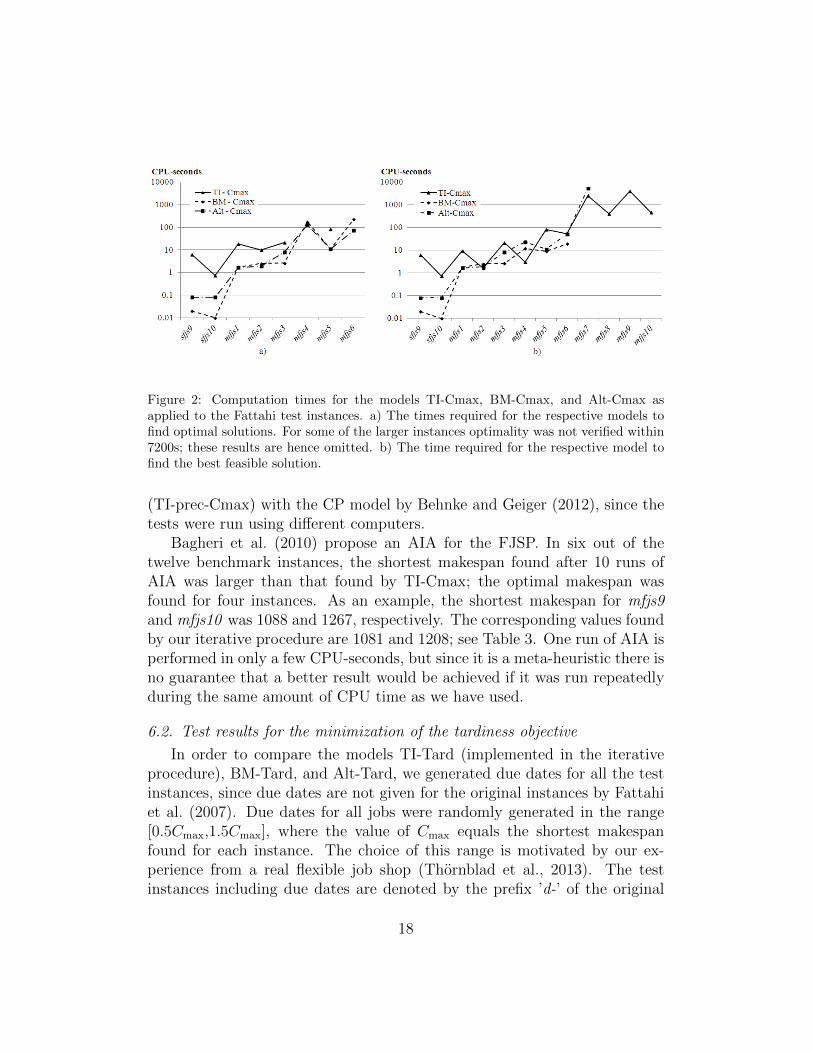
Figure 2: Computation times for the models TI-Cmax, BM-Cmax, and Alt-Cmax asapplied to the Fattahi test instances. a) The times required for the respective models tofind optimal solutions. For some of the larger instances optimality was not verified within7200s; these results are hence omitted. b) The time required for the respective model tofind the best feasible solution.

(TI-prec-Cmax) with the CP model by Behnke and Geiger (2012), since thetests were run using different computers.

Bagheri et al. (2010) propose an AIA for the FJSP. In six out of thetwelve benchmark instances, the shortest makespan found after 10 runs ofAIA was larger than that found by TI-Cmax; the optimal makespan wasfound for four instances. As an example, the shortest makespan for mfjs9and mfjs10 was 1088 and 1267, respectively. The corresponding values foundby our iterative procedure are 1081 and 1208; see Table 3. One run of AIA isperformed in only a few CPU-seconds, but since it is a meta-heuristic there isno guarantee that a better result would be achieved if it was run repeatedlyduring the same amount of CPU time as we have used.

6.2. Test results for the minimization of the tardiness objective

In order to compare the models TI-Tard (implemented in the iterativeprocedure), BM-Tard, and Alt-Tard, we generated due dates for all the testinstances, since due dates are not given for the original instances by Fattahiet al. (2007). Due dates for all jobs were randomly generated in the range[0.5Cmax,1.5Cmax], where the value of Cmax equals the shortest makespanfound for each instance. The choice of this range is motivated by our ex-perience from a real flexible job shop (Thornblad et al., 2013). The testinstances including due dates are denoted by the prefix ’d-’ of the original

18

name of each instance. The objective weights for the completion times usedin the computations are αj = 1, j ∈ J . The tardiness weights βj, j ∈ J ,are computed according to (8), with B = 10, such that 0 ≤ βj ≤ 20 holdsfor all j ∈ J . In Figure 3, the computation times required for the threemodels to solve the test instances generated are plotted. For the medium

Figure 3: a) The computation times required for solving the models TI-Tard, BM-Tard,and Alt-Tard to optimality for the Fattahi test instances including due dates. For someof the larger instances optimality was not verified within the time limit of 7200s and aretherefore not shown.b) The time required to find the best feasible solution for the models TI-Tard, BM-Tard,and Alt-Tard.

sized instances, all three models require almost the same computation times.As expected, TI-Tard is not competitive for the smallest instances, since itis solved in several steps. Only Alt-Tard reaches optimality for the instancesd-mfjs7–8.

In Table 4, the results are listed for the four largest instances. As for thecase with the makespan objective, the best objective values were found byour iterative procedure implemented with TI-Tard. It outperforms the othermodels regarding the time to find the best solution for all instances except forthe two smallest ones, see Figure 3b); the iterative procedure with TI-Tardwas on average more than 60 times faster than BM-Tard and Alt-Tard withrespect to the time to find the best solution.

When considering the tardiness objective, the reduced models constructedby the solver in the presolve phase contain on average 19% more constraintsand 14% more variables for the BM-Tard model compared with the Alt-Tardmodel. Hence the presolve phase is not able to reduce all the redundant

19

Table 4: Computational results for the largest instances d-mfjs7-10. The best results foreach instance are written in bold and ’*’ in the mipgap column indicates that optimalityis verified. The values within parentheses denote the CPU times to compute the bestmakespan found by that model, for the cases when a shorter makespan was found byanother model for the corresponding instance.

Iterative procedure

TI-Tard BM-Tard Alt-Tard

Instance CPU Time Obj mip- CPU Time Obj mip- CPU Time Obj mip-

time to best value gap time to best value gap time to best value gap

(s) (s) (%) (s) (s) (%) (s) (s) (%)

d-mfjs7 7592 14 35111.1 3.9 7593 (795) 35244.9 2.8 1894 1740 35111.1 *

d-mfjs8 7292 70 25225.3 1.4 7593 (6870) 25240.0 4.2 3801 3710 25225.3 *

d-mfjs9 15568 1142 60159.5 4.4 15569 (7200) 63175.4 24.7 15690 (7200) 60420.3 21.9

d-mfjs10 10260 236 45568.4 2.6 10261 (9600) 46532.4 21.0 10344 (6850) 47215.7 21.1

variables of the BM-Tard model, as was the case for the BM-Cmax model.On the other hand, TI-Tard contains 17 times more constraints and 77 timesmore variables than BM-Tard in the reduced problem for `s = 1. Neverthe-less, TI-Tard is competitive with the Alt-Tard and BM-Tard regarding thecomputation time to verify optimality and outperforms these models regard-ing the time to find the best solution for all instances tested, except for thetwo smallest ones; see Figure 3.

In Figure 4, the best feasible solution found by each of the models iscompared with its best lower bound, for the instances mfjs7–10 and d-mfjs7–10, respectively. For each instance, the values are divided by the objectivevalue of the best solution found (by TI-Cmax and TI-Tard, respectively). InFigure 4, we note that there is a large difference between the lower boundsfound by employing the makepan objective and those found by employingthe tardiness objective. This indicates that the performance of a model isdependent on the objective used. TI-Cmax performs equally good (or bad)regarding the lower bounds as do the models BM-Cmax and Alt-Cmax, whileTI-Tard outperforms the models BM-Tard and Alt-Tard for the instances d-mfjs9-10 by finding significantly better lower bounds.

7. Conclusions

We have demonstrated that there is a large difference in the performanceof the scheduling models depending on which objective is considered. Hence,it is important to evaluate scheduling models with respect to objectives thatare well suited for the real applications for which they are intended. Since

20

Figure 4: The values of the best feasible solutions (upper marker) and the best lowerbounds (lower marker) found. a) Values for the instances mfjs7–10 found by the modelsTI-Cmax, BM-Cmax, and Alt-Cmax, normalized by the value of the best solution found byTI-Cmax. b) Values for the instances d-mfjs7–10 found by the models TI-Tard, BM-Tard,and Alt-Tard, normalized by the value of the best solution found by TI-Tard.

most real flexible job shops are parts of longer supply chains with ongoingproduction, it must be prioritized that production should be predictable andaccording to plan. In Section 4, we argue that an objective that targets duedates will serve to control the flow and stabilize its pace, while the objectiveof minimizing the makespan risk to exacerbate a possibly already unreliableflow.

We have shown that the time-indexed model (despite its large numbersof variables and constraints), combined with the iterative algorithm pro-posed is able to find significantly better feasible solutions for the largestinstances than both the other models, considering both objectives studied.The scheduling method proposed outperforms the other models regarding thetime required to find the best feasible solution. We have also presented analternative model, similar to the benchmark model but with fewer variablesand constraints. This model is the only one that is able to solve two of thelarge instances when minimizing the tardiness objective. It seems, however,worthwhile to implement the iterative algorithm proposed for medium andlarge sized instances, since it is able to quickly find solutions of high quality.The proposed scheduling method typically finds good feasible solutions in anearly iteration, employing relatively long time steps; after squeezing, thesesolutions are, actually, often optimal or near-optimal. The verification of op-

21

timality can, however, only be made in a later iteration when all parameterdata can be expressed as multiples of the length of the time steps. Our find-ings imply that our new procedure can be beneficially utilized for schedulingreal flexible job shops.

8. Acknowledgements

A special thanks to Thomas Ericsson at the Department of MathematicalSciences, for all support regarding the computations. Furthermore, we wouldlike to gratefully acknowledge the financial support from GKN Aerospace En-gine Systems (formerly Volvo Aero), The Swedish Research Council (grantno. 621-2007-4716), NFFP (Swedish National Aeronautics Research Pro-gramme), and VINNOVA (through Chalmers Transport Area of Advance).

References

Al-Hinai, N., ElMekkawy, T. Y., 2011. An efficient hybridized genetic algo-rithm architecture for the flexible job shop scheduling problem. FlexibleServices and Manufacturing Journal 23, 64–85.

Bagheri, A., Zandieh, M., Mahdavi, I., Yazdani, M., 2010. An artificial im-mune algorithm for the flexible job-shop scheduling problem. Future Gen-eration Computer Systems 26 (4), 533–541.

Baykasoglu, A., Ozbakir, L., 2010. Analyzing the effect of dispatching rulesin the scheduling performance through grammar based flexible schedulingsystem. International Journal of Production Economics 124 (2), 269–381.

Behnke, D., Geiger, M. J., 2012. Test instances for the flexiblejob shop scheduling problem with work centers. http://www.nbn-

resolving.de/urn:nbn:de:gbv:705-opus-29827 (Accessed on August 13,2013).

Berghman, L., 2012. Machine scheduling models for warehousing dockingoperations. PhD Thesis, Katholieke Universiteit Leuven, Belgium.

Brucker, P., Knust, S., 2012. Complex Scheduling, 2nd Edition. Springer-Verlag, Berlin, Germany.

22

Demir, Y., Isleyen, S. K., 2013. Evaluation of mathematical models for flex-ible job-shop scheduling problems. Applied Mathematical Modelling 37,977–988.

Fattahi, P., Saidi Mehrabad, M., Jolai, F., 2007. Mathematical modeling andheuristic approaches to flexible job shop scheduling problems. Journal ofIntelligent Manufacturing 18 (3), 331–342.

Fourer, R., Gay, D. M., Kernighan, B. W., 2002. AMPL: A Modeling Lan-guage for Mathematical Programming, 2nd Edition. Brooks/Cole Publish-ing Company/Cengage Learning.

IBM Corp., 2009. IBM ILOG CPLEX V12.1 User’s Manual for CPLEX.

Jain, A. S., Meeran, S., 1999. Deterministic job-shop scheduling: Past,present and future. European Journal of Operational Research 113 (2),390–434.

Low, C., Yip, Y., Wu, T., 2006. Modelling and heuristics of FMS schedulingwith multiple objectives. Computers & Operations Research 33 (3), 674–694.

Manne, A. S., 1960. On the job-shop scheduling problem. Operations Re-search 8 (2), 219–223.

MATLAB, 2011. Release 2011b. The MathWorks Inc., Natick, MA, UnitedStates.

Nemhauser, G. L., Wolsey, L. A., 1988. Integer and Combinatorial Optimiza-tion. John Wiley & Sons, Inc., New York, NY, USA.

Ozguven, C., Ozbakir, L., Yavuz, Y., 2010. Mathematical models for job-shop scheduling problems with routing and process plan flexibility. AppliedMathematical Modelling 34 (2), 1539–1548.

Sadykov, R., Wolsey, L. A., 2006. Integer programming and constraint pro-gramming in solving a multimachine assignment scheduling problem withdeadlines and release dates. INFORMS Journal on Computing 18, 209–217.

Thornblad, K., Sep. 2011. On the optimization of schedules of a multitaskproduction cell. Licentiate Thesis, Chalmers University of Technology andUniversity of Gothenburg, Goteborg, Sweden.

23

Thornblad, K., Stromberg, A.-B., Patriksson, M., Almgren, T., 2013.Scheduling optimization of a real flexible job shop including fixture avail-ability and preventive maintenance. Revised for publication in EuropeanJournal of Industrial Engineering.

van den Akker, J. M., Hurkens, C. A. J., Savelsberg, M. W. P., 2000. Time-indexed formulations for machine scheduling problems: Column genera-tion. INFORMS Journal on Computing 12, 111–124.

Wang, L., Zhou, G., Xu, Y., Wang, S., Liu, M., 2012. An effective artificialbee colony algorithm for the flexible job-shop scheduling problem. TheInternational Journal of Advanced Manufacturing Technology 60, 303–315.

24