A Comparison of Sorting Algorithms

for the Connection Machine CM-2

Guy E. Blelloch, Charles E. Leiserson, Bruce M. Maggs,

C. Greg Plaxton, Stephen J. Smith, and Marco Zagha

Sorting is arguably the most studied problem in computer science, both because it is used as a substep in manyapplications and because it is a simple, combinatorial problem with many interesting and diverse solutions. Sortingis also an important benchmark for parallel supercomputers. It requires significant communication bandwidthamong processors, unlike many other supercomputer benchmarks, and the most efficient sorting algorithms com-municate data in irregular patterns.

Parallel algorithms for sorting have been studied since at least the 1960’s. An early advance in parallel sort-ing came in 1968 when Batcher discovered the elegant U(lg2 n)-depth bitonic sorting network [3]. For certain fam-ilies of fixed interconnection networks, such as the hypercube and shuffle-exchange, Batcher’s bitonic sorting tech-nique provides a parallel algorithm for sorting n numbers in U(lg2 n) time with n processors. The question of exis-tence of a o(lg2 n)-depth sorting network remained open until 1983, when Ajtai, Komlós, and Szemerédi [1] pro-vided an optimal U(lg n)-depth sorting network, but unfortunately, their construction leads to larger networks thanthose given by bitonic sort for all “practical” values of n. Leighton [15] has shown that any U(lg n)-depth familyof sorting networks can be used to sort n numbers in U(lg n) time in the bounded-degree fixed interconnection net-work domain. Not surprisingly, the optimal U(lg n)-time fixed interconnection sorting networks implied by theAKS construction are also impractical.

In 1983, Reif and Valiant proposed a more practical O(lg n)-time randomized algorithm for sorting [19],called flashsort. Many other parallel sorting algorithms have been proposed in the literature, including parallel ver-sions of radix sort and quicksort [5], a variant of quicksort called hyperquicksort [23], smoothsort [18], columnsort [15], Nassimi and Sahni’s sort [17], and parallel merge sort [6].

This paper reports the findings of a project undertaken at Thinking Machines Corporation to develop a fastsorting algorithm for the Connection Machine Supercomputer model CM-2. The primary goals of this projectwere:

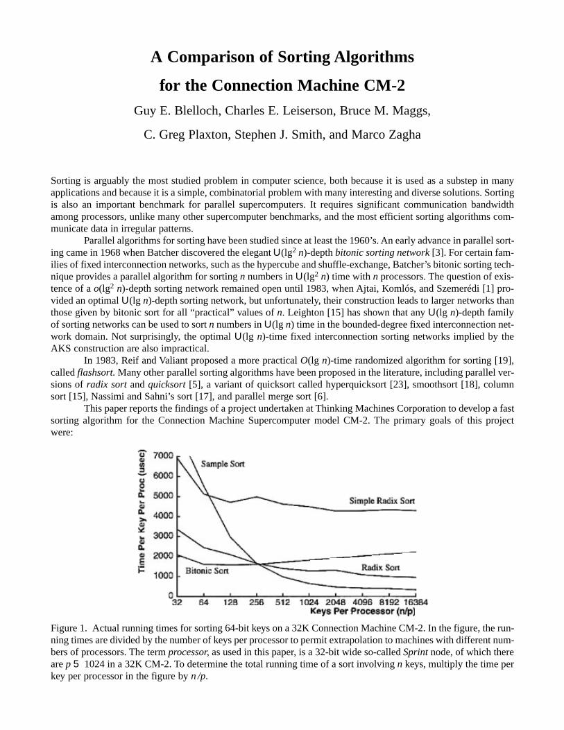
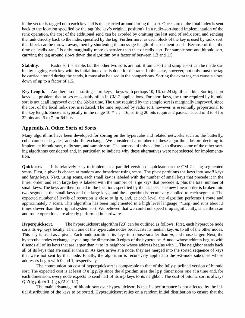
Figure 1. Actual running times for sorting 64-bit keys on a 32K Connection Machine CM-2. In the figure, the run-ning times are divided by the number of keys per processor to permit extrapolation to machines with different num-bers of processors. The term processor, as used in this paper, is a 32-bit wide so-called Sprint node, of which thereare p 5 1024 in a 32K CM-2. To determine the total running time of a sort involving n keys, multiply the time perkey per processor in the figure by n /p.

1. To implement as fast a sorting algorithm as possible for integers and floating-point numbers on the CM-2,

2. To generate a library sort for the CM-2 (here we were concerned with memory use, stability, and perfor-mance over a wide range of problem and key sizes in addition to running time), and

3. To gain insight into practical sorting algorithms in general.

Our first step towards achieving these goals was to analyze and evaluate many of the parallel sorting algorithmsthat have been proposed in the literature. After analyzing many algorithms, we selected the three most promisingalternatives for implementation: bitonic sort, radix sort, and sample sort. Figure 1 compares the running times ofthese three algorithms (two versions of radix sort are shown). As is apparent from the figure, when the number ofkeys per processor (n /p) is large, sample sort is the fastest sorting algorithm. On the other hand, radix sort per-forms reasonably well over the entire range of n/p, and it is deterministic, much simpler to code, stable, and fasterwith small keys. Although bitonic sort is the slowest of the three sorts when n/p is large, it is more space-efficientthan the other two algorithms, and represents the fastest alternative when n/p is small. Based on various pragmat-ic issues, the radix sort was selected to be used as the library sort for Fortran now available on the CM-2.

We have modeled the running times of our sorts using equations based on problem size, number of proces-sors, and a set of machine parameters (i.e. time for point-to-point communication, hypercube communication,scans, and local operations). These equations serve several purposes. First, they make it easy to analyze how muchtime is spent in various parts of the algorithms. For example one can quickly determine the ratio of computationto communication for each algorithm and see how this is affected by problem and machine size. Second, they makeit easy to generate good estimates of running times on variations of the algorithms without having to implementthem. Third, one can determine how various improvements in the architecture would improve the running times ofthe algorithms. For example, the equations make it easy to determine the effect of doubling the performance ofmessage routing. Fourth, in the case of radix sort we are able to use the equations to analytically determine the bestradix size as a function of the problem size. Finally, the equations allow anyone to make reasonable estimates ofthe running times of the algorithms on other machines. For example, the radix sort has been implemented and ana-lyzed on the Cray Y-MP [25], and the CM-5 [22], which differ significantly from the CM-2. In both cases, whenappropriate values for the machine parameters are used, our equations accurately predicted the running times.Similar equations are used by Stricker [21] to analyze the running time of bitonic sort on the iWarp, and byHightower, Prins and Reif [12] to analyze the running time of flashsort on the Maspar MP-1.

The remainder of this paper studies the implementations of bitonic sort, radix sort, and sample sort. In eachcase, it describes and analyzes the basic algorithm, as well as any enhancements and/or minor modifications thatwe introduced to optimize performance. After describing the model we use for the CM-2, we present our studiesof bitonic sort, radix sort, and sample sort, respectively. In Section 6, we compare the relative performance of thesethree sorts, not only in terms of running time, but also with respect to such criteria as stability and space. AppendixA presents a brief analysis of other algorithms that we considered for implementation. Appendix B presents a prob-abilistic analysis of the sampling procedure used in our sample sort algorithm.

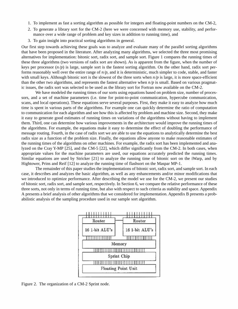
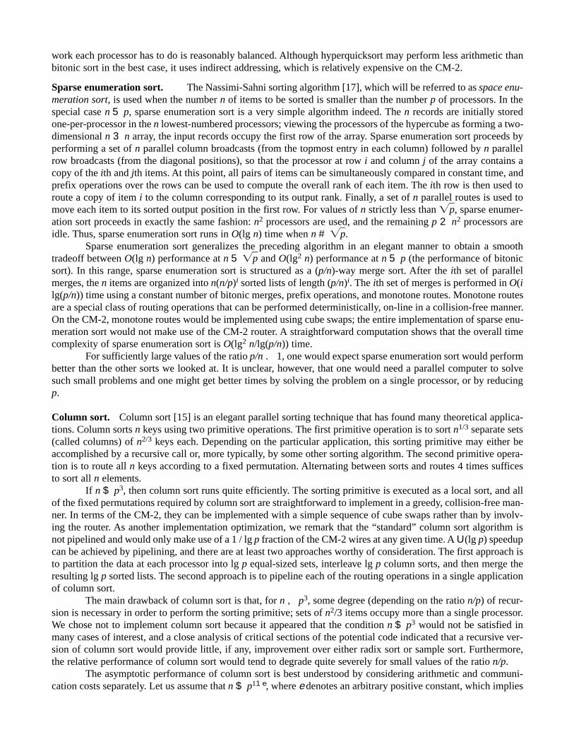
Figure 2. The organization of a CM-2 Sprint node.

The Connection MachineThis section describes the CM-2 Connection Machine and defines an abstract model of the machine which is usedto describe all of the algorithms in this paper. By describing a particular algorithm in terms of the abstract model,the analysis can be applied to other parallel machines, and approximate run-times can be derived.

The CM-2 is a single-instruction multiple-data (SIMD) computer. In its full 64K-processor configuration,it can be viewed as 2048 (211) Sprint nodes configured as an 11-dimensional hypercube with multiport capability:all dimensions of the hypercube can be used at the same time. The Sprint nodes are controlled by a front-endprocessor (typically a Sun4 or Vax). Figure 2 illustrates the organization of a Sprint node, which consists of thefollowing chips:

• Two processor chips, each containing 16 1-bit processors, a 1-bit bidirectional wire to each of up to11 neighboring nodes in the hypercube, and hardware for routing support.

• Ten DRAM chips, containing a total of between 256K bytes and 4M bytes of error-corrected mem-ory, depending on the configuration. All recent machines contain at least 1M bytes of memory pernode.

• A floating-point chip (FPU) capable of 32-bit and 64-bit floating-point arithmetic, as well as 32-bitinteger arithmetic.

• A Sprint chip that serves as an interface between the memory and the floating-point chip. The Sprintchip contains 128 32-bit registers and has the capability to convert data from the bit-serial formatused by the 1-bit processors to the 32-bit word format used by the floating-point chip.

In this paper, we view each Sprint node as a single processor, rather than considering each of the 64K 1-bit processors on a fully configured CM-2 as separate processors. This point of view makes it easier to extrapolateour results on the CM-2 to other hypercube machines, which typically have 32 or 64-bit processors. Furthermore,it is closer to the way in which we viewed the machine when implementing the sorting algorithms.

We break the primitive operations of the CM-2 into four classes:

• Arithmetic: A local arithmetic or logical operation on each processor (Sprint node). Also includedare global operations involving the front end and processors, such as broadcasting a word from thefront end to all processors.

• Cube Swap: Each processor sends and receives 11 messages, one each across the 11 dimensions ofthe hypercube. The CM-2 is capable of sending messages across all hypercube wires simultaneous-ly.

• Send: Each processor sends one message to any other processor through the routing network. In thispaper we use two types of sends: a single-destination send, and a send-to-queue. In the single-des-tination send (used in our radix-sort) messages are sent to a particular address within a particularprocessor, and no messages may have the same destination. In the send-to-queue (used in our sam-ple sort) messages are sent to a particular processor and are placed in a queue in the order they arereceived. The CM-2 also supports combining sends.

• Scan: A parallel-prefix (or suffix) computation on integers, one per processor. Scans operate on avector of input values using an associative binary operator such as integer addition. (The only oper-ator employed by our algorithms is addition.) As output, the scan returns a vector in which each posi-tion has the “sum,” according to the operator, of those input values in lesser positions. For example,a plus-scan (integer addition as the operator) of the vector

. [4 7 1 0 5 2 6 4 8 1 9 5]

yields

[0 4 11 12 12 17 19 25 29 37 38 47]

as the result of the scan.

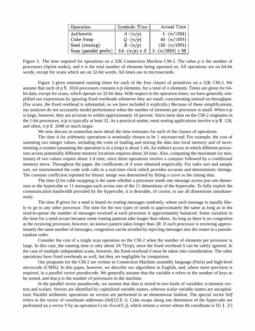
Figure 3 gives estimated running times for each of the four classes of primitives on a 32K CM-2. Weassume that each of p 5 1024 processors contains n/p elements, for a total of n elements. Times are given for 64-bit data, except for scans, which operate on 32-bit data. With respect to the operation times, we have generally sim-plified our expressions by ignoring fixed overheads whenever they are small, concentrating instead on throughput.(For scans, the fixed overhead is substantial, so we have included it explicitly.) Because of these simplifications,our analyses do not accurately model performance when the number of elements per processor is small. When n/pis large, however, they are accurate to within approximately 10 percent. Since most data on the CM-2 originates inthe 1-bit processors, n/p is typically at least 32. As a practical matter, most sorting applications involve n/p $ 128,and often, n/p 5 2048 or much larger.

We now discuss in somewhat more detail the time estimates for each of the classes of operations.The time A for arithmetic operations is nominally chosen to be 1 microsecond. For example, the cost of

summing two integer values, including the costs of loading and storing the data into local memory and of incre-menting a counter (assuming the operation is in a loop) is about 1.4A. An indirect access in which different proces-sors access potentially different memory locations requires about 3A time. Also, computing the maximum (or min-imum) of two values require about 3 A time, since these operations involve a compare followed by a conditionalmemory move. Throughout the paper, the coefficients of A were obtained empirically. For radix sort and samplesort, we instrumented the code with calls to a real-time clock which provides accurate and deterministic timings.The constant coefficient reported for bitonic merge was determined by fitting a curve to the timing data.

The time Q for cube swapping is the same whether a processor sends one message across just one dimen-sion or the hypercube or 11 messages each across one of the 11 dimensions of the hypercube. To fully exploit thecommunication bandwidth provided by the hypercube, it is desirable, of course, to use all dimensions simultane-ously.

The time R given for a send is based on routing messages randomly, where each message is equally like-ly to go to any other processor. The time for the two types of sends is approximately the same as long as in thesend-to-queue the number of messages received at each processor is approximately balanced. Some variation inthe time for a send occurs because some routing patterns take longer than others. As long as there is no congestionat the receiving processor, however, no known pattern takes longer than 2R. If each processor is receiving approx-imately the same number of messages, congestion can be avoided by injecting messages into the router in a pseudo-random order.

Consider the cost of a single scan operation on the CM-2 when the number of elements per processor islarge. In this case, the running time is only about 3A ? (n/p), since the fixed overhead S can be safely ignored. Inthe case of multiple independent scans, however, the fixed overhead S must be taken into consideration. The otheroperations have fixed overheads as well, but they are negligible by comparison.

Our programs for the CM-2 are written in Connection Machine assembly language (Paris) and high-levelmicrocode (CMIS). In this paper, however, we describe our algorithms in English, and, where more precision isrequired, in a parallel vector pseudocode. We generally assume that the variable n refers to the number of keys tobe sorted, and that p is the number of processors in the machine.

In the parallel vector pseudocode, we assume that data is stored in two kinds of variables: n-element vec-tors and scalars. Vectors are identified by capitalized variable names, whereas scalar variable names are uncapital-ized. Parallel arithmetic operations on vectors are performed in an elementwise fashion. The special vector Selfrefers to the vector of coordinate addresses (Self [i] 5 i). Cube swaps along one dimension of the hypercube areperformed on a vector V by an operation CUBE-SWAP(V, j), which returns a vector whose ith coordinate is V[i 1 2j]

Figure 3. The time required for operations on a 32K Connection Machine CM-2. The value p is the number ofprocessors (Sprint nodes), and n is the total number of elements being operated on. All operations are on 64-bitwords, except for scans which are on 32-bit words. All times are in microseconds.

if the jth bit of i (in binary) is 0, and V[i 2 2j ] if the jth bit of i is 1. Cube swaps along all dimensions simultane-ously are described in English. Routing is accomplished by the operation SEND(V, Dest), which returns the vectorwhose ith coordinate is that V[j] such that Dest[j] 5 i. Scan operations are performed by a procedure SCAN(V) thatreturns the plus-scan of the vector.

Batcher’s Bitonic SortBatcher’s bitonic sort [3] is a parallel merge sort that is based upon an efficient technique for merging so-called“bitonic” sequences. A bitonic sequence is one that increases monotonically and then decreases monotonically, orcan be circularly shifted to become so. One of the earliest sorts, bitonic sort was considered to be the most practi-cal parallel sorting algorithm for many years. The theoretical running time of the sort is U(lg2 n), where the con-stant hidden by U is small. Moreover, bitonic sort makes use of a simple fixed communication pattern that mapsdirectly to the edges of the hypercube; a general routing primitive need not be invoked when bitonic sort is imple-mented on the hypercube.

In this section, we discuss our implementation of bitonic sort. The basic algorithm runs efficiently on ahypercube architecture, but uses only one dimension of the hypercube wires at a time. The CM-2 hypercube hasmultiport capability, however, and by pipelining the algorithm, it is possible to make efficient use of all hypercubewires at once. This optimization results in a 5-fold speedup of the communication and over a 2-fold speedup in thetotal running time of the algorithm. Even with this optimization, the other two algorithms that we implementedoutperform bitonic sort when the number n/p of keys per processor is large. When n/p is small, however, bitonicsort is the fastest of the three, and uses considerably less space than the other two.

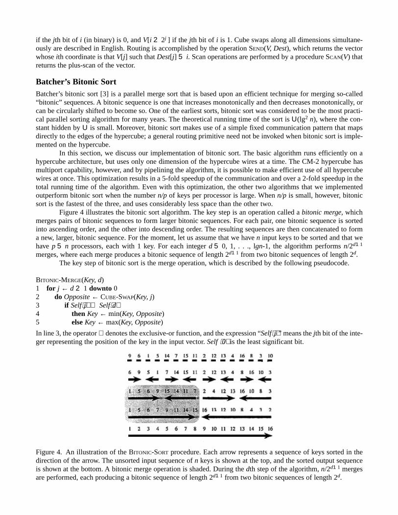
Figure 4 illustrates the bitonic sort algorithm. The key step is an operation called a bitonic merge, whichmerges pairs of bitonic sequences to form larger bitonic sequences. For each pair, one bitonic sequence is sortedinto ascending order, and the other into descending order. The resulting sequences are then concatenated to forma new, larger, bitonic sequence. For the moment, let us assume that we have n input keys to be sorted and that wehave p 5 n processors, each with 1 key. For each integer d 5 0, 1, . . ., lgn-1, the algorithm performs n/2d11

merges, where each merge produces a bitonic sequence of length 2d11 from two bitonic sequences of length 2d.The key step of bitonic sort is the merge operation, which is described by the following pseudocode.

BITONIC-MERGE(Key, d)1 for j ← d 2 1 downto 02 do Opposite ← CUBE-SWAP(Key, j)3 if Self⟨j⟩ ⊕ Self⟨d⟩4 then Key ← min(Key, Opposite)5 else Key ← max(Key, Opposite)

In line 3, the operator ⊕ denotes the exclusive-or function, and the expression “Self⟨ j⟩” means the jth bit of the inte-ger representing the position of the key in the input vector. Self ⟨0⟩ is the least significant bit.

Figure 4. An illustration of the BITONIC-SORT procedure. Each arrow represents a sequence of keys sorted in thedirection of the arrow. The unsorted input sequence of n keys is shown at the top, and the sorted output sequenceis shown at the bottom. A bitonic merge operation is shaded. During the dth step of the algorithm, n/2d11 mergesare performed, each producing a bitonic sequence of length 2d11 from two bitonic sequences of length 2d.

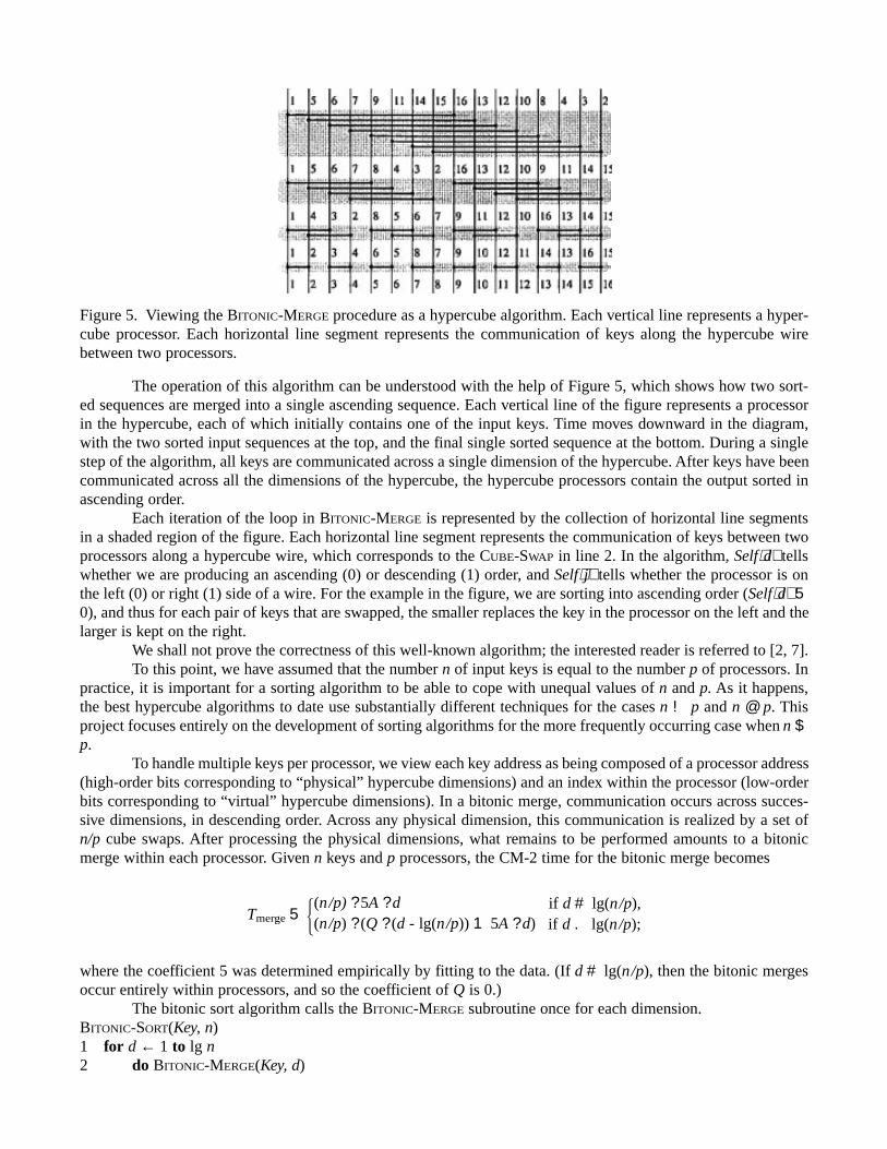
The operation of this algorithm can be understood with the help of Figure 5, which shows how two sort-ed sequences are merged into a single ascending sequence. Each vertical line of the figure represents a processorin the hypercube, each of which initially contains one of the input keys. Time moves downward in the diagram,with the two sorted input sequences at the top, and the final single sorted sequence at the bottom. During a singlestep of the algorithm, all keys are communicated across a single dimension of the hypercube. After keys have beencommunicated across all the dimensions of the hypercube, the hypercube processors contain the output sorted inascending order.

Each iteration of the loop in BITONIC-MERGE is represented by the collection of horizontal line segmentsin a shaded region of the figure. Each horizontal line segment represents the communication of keys between twoprocessors along a hypercube wire, which corresponds to the CUBE-SWAP in line 2. In the algorithm, Self⟨d⟩ tellswhether we are producing an ascending (0) or descending (1) order, and Self⟨ j⟩ tells whether the processor is onthe left (0) or right (1) side of a wire. For the example in the figure, we are sorting into ascending order (Self⟨d⟩ 50), and thus for each pair of keys that are swapped, the smaller replaces the key in the processor on the left and thelarger is kept on the right.

We shall not prove the correctness of this well-known algorithm; the interested reader is referred to [2, 7].To this point, we have assumed that the number n of input keys is equal to the number p of processors. In

practice, it is important for a sorting algorithm to be able to cope with unequal values of n and p. As it happens,the best hypercube algorithms to date use substantially different techniques for the cases n ! p and n @ p. Thisproject focuses entirely on the development of sorting algorithms for the more frequently occurring case when n $p.

To handle multiple keys per processor, we view each key address as being composed of a processor address(high-order bits corresponding to “physical” hypercube dimensions) and an index within the processor (low-orderbits corresponding to “virtual” hypercube dimensions). In a bitonic merge, communication occurs across succes-sive dimensions, in descending order. Across any physical dimension, this communication is realized by a set ofn/p cube swaps. After processing the physical dimensions, what remains to be performed amounts to a bitonicmerge within each processor. Given n keys and p processors, the CM-2 time for the bitonic merge becomes

Tmerge 5 5where the coefficient 5 was determined empirically by fitting to the data. (If d # lg(n/p), then the bitonic mergesoccur entirely within processors, and so the coefficient of Q is 0.)

The bitonic sort algorithm calls the BITONIC-MERGE subroutine once for each dimension.BITONIC-SORT(Key, n)1 for d ← 1 to lg n2 do BITONIC-MERGE(Key, d)

if d # lg(n/p),if d . lg(n/p);

(n/p) ? 5A ? d(n/p) ? (Q ? (d - lg(n/p)) 1 5A ? d)

Figure 5. Viewing the BITONIC-MERGE procedure as a hypercube algorithm. Each vertical line represents a hyper-cube processor. Each horizontal line segment represents the communication of keys along the hypercube wirebetween two processors.

The time taken by the algorithm is

5 Q ? (n/p)(lg p)(lg p 1 1)/2 1 5A ? (n/p)(lg n)(lg n 1 1)/2< 0.5Q ? (n/p) lg2 p 1 2.5A ? (n/p) lg2 n. (1)

Let us examine this formula more closely. The times in Figure 3 indicate that Q is 40 times larger than A, and lg nis at most 2 or 3 times larger than lg p for all but enormous volumes of data. Thus, the first term in formula (1),corresponding to communication time, dominates the arithmetic time for practical values of n and p.

The problem with this naive implementation is that it is a single-port algorithm: communication occursacross only one dimension of the hypercube at a time. By using all of the dimensions virtually all of the time, wecan improve the algorithm’s performance significantly. The idea is to use a multiport version of BITONIC-MERGE

that pipelines the keys across all dimensions of the hypercube. In the multiport version, a call of the form BITONIC-MERGE(Key, d) is implemented as follows. On the first step, all processors cube swap their first keys across dimen-sion d. On the second step, they cube swap their first keys across dimension d 2 1, while simultaneously cubeswapping their second keys across dimension d. Continuing the pipelining in this manner, the total number of stepsto move all the keys through d - lg(n/p) physical dimensions is n/p 1 d 2 lg(n/p) 2 1. This algorithm is essen-tially equivalent to a pipelined bitonic merge on a butterfly network.

Thus, pipelining improves the time for bitonic merging to

Tmultiport-merge 5 5By summing from d 5 1 to lg n, the time for the entire multiport bitonic sort, therefore, becomes

Tmultiport-bitonic 5 Q ? (lg p)(n/p 1 (lg p)/2 2 1/2) 1 5A ? (n/p)(lg n)(lg n 1 1)/2

< Q ? ((n/p) lg p 1 0.5 lg2 p) 1 2.5A ? (n/p) lg2 n. (2)

Let us compare this formula with the single-port result of equation (1). For n 5 O(p), the two runningtimes do not differ by more than a constant factor. For n 5 V(p log p), however, the coefficient of Q is U(log p)times smaller in the multiport case. Thus, total communication time is considerably reduced by pipelining whenn/p is large. The number of arithmetic operations is not affected by pipelining.

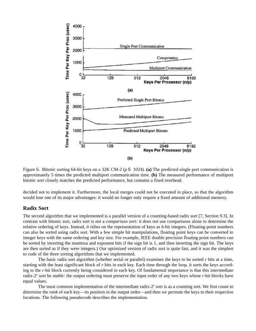
Figure 6a shows the communication and computation components of the running time for both the single-port and multiport versions of bitonic sort. These times are generated from formulas (1) and (2). The computationcomponent is equivalent for both algorithms. Figure 6b shows the predicted total time for the single-port and mul-tiport bitonic, and the measured performance of our implementation of the multiport algorithm. The differencebetween predicted and measured times for small values of n/p is mostly due to the fact that our equations ignoreconstant overhead. The difference at high n/p is due to some overhead in our implementation caused by addition-al memory moves, effectively increasing the cost Q of the cube swap. This overhead could be eliminated by animproved implementation, but the resulting algorithm would still not be competitive with sample sort for large val-ues of n/p.

Multiport bitonic sort can be further improved by using a linear-time serial merge instead of a bitonicmerge in order to execute the merges that occur entirely within a processor [4, 14]. This variation yields a runningtime of

Tmultiport-bitonic < Q ? ((n/p) lg p 1 0.5 lg2 p) 1 A ? (n/p)(2.5 lg2 p 1 10 lg n),

where the constant 10 is an estimate. This constant is large because of the indirect addressing that would berequired by the implementation. For large n/p, this formula reduces the A term relative to equation (2). Once again,this improvement would not yield an algorithm that is close to the performance of the sample sort, and thus we

if d # lg(n/p),if d . lg(n/p).

(n/p) ? 5A ? dQ ? (n/p 1 d 2 lg(n/p) 2 1) 1 5A ? (n/p)d

decided not to implement it. Furthermore, the local merges could not be executed in place, so that the algorithmwould lose one of its major advantages: it would no longer only require a fixed amount of additional memory.

Radix SortThe second algorithm that we implemented is a parallel version of a counting-based radix sort [7, Section 9.3]. Incontrast with bitonic sort, radix sort is not a comparison sort: it does not use comparisons alone to determine therelative ordering of keys. Instead, it relies on the representation of keys as b-bit integers. (Floating-point numberscan also be sorted using radix sort. With a few simple bit manipulations, floating point keys can be converted tointeger keys with the same ordering and key size. For example, IEEE double precision floating point numbers canbe sorted by inverting the mantissa and exponent bits if the sign bit is 1, and then inverting the sign bit. The keysare then sorted as if they were integers.) Our optimized version of radix sort is quite fast, and it was the simplestto code of the three sorting algorithms that we implemented.

The basic radix sort algorithm (whether serial or parallel) examines the keys to be sorted r bits at a time,starting with the least significant block of r bits in each key. Each time through the loop, it sorts the keys accord-ing to the r-bit block currently being considered in each key. Of fundamental importance is that this intermediateradix-2r sort be stable: the output ordering must preserve the input order of any two keys whose r-bit blocks haveequal values.

The most common implementation of the intermediate radix-2r sort is as a counting sort. We first count todetermine the rank of each key—its position in the output order—and then we permute the keys to their respectivelocations. The following pseudocode describes the implementation.

Figure 6. Bitonic sorting 64-bit keys on a 32K CM-2 (p 5 1024). (a) The predicted single port communication isapproximately 5 times the predicted multiport communication time. (b) The measured performance of multiportbitonic sort closely matches the predicted performance, but contains a fixed overhead.

RADIX-SORT(Key)1 for i r 0 to b 2 1 by r2 do Rank r COUNTING-RANK(r, Keyi,. . .,i 1 r - 1>)3 Key r SEND(Key, Rank)

Since the algorithm requires b/r passes, the total time for a parallel sort is:

Tradix 5 (b/r) ? (R ? (n/p) 1 Trank)

where Trank is the time taken by COUNTING-RANK.The most interesting part of radix sort is the subroutine for computing ranks called in line 2. We first con-

sider the simple algorithm underlying the original Connection Machine library sort [5], which was programmed byone of us several years ago. In the following implementation of COUNTING-RANK, the vector Block holds the r-bitvalues on which we are sorting.

SIMPLE-COUNTING-RANK(r, Block)1 offset r 02 for k r 0 to 2r 2 13 do Flag r 04 where Block 5 k do Flag r 15 Index r SCAN(Flag)6 where Flag do Rank r offset 1 Index7 offset r offset 1 SUM(Flag)8 return Rank

In this pseudocode, the where statement executes its body only in those processors for which the condition evalu-ates to TRUE.

The SIMPLE-COUNTING-RANK procedure operates as follows. Consider the ith key, and assume thatBlock[i] 5 k. The rank of the ith key is the number offsetk of keys j for which Block[j] , k, plus the number Index[i]of keys for which Block[j] 5 k and j , i. (Here, offsetk is the value of offset at the beginning of the kth iteration ofthe for loop.) The code iterates over each of the 2r possible values that can be taken on by the r-bit block on whichwe are sorting. For each value of k, the algorithm uses a scan to generate the vector Index and updates the value ofoffset to reflect the total number of keys whose Block value is less than or equal to k.

To compute the running time of SIMPLE-COUNTING-RANK, we refer to the running times of the CM-2 oper-ations in Figure 3. On the CM-2, the SUM function can be computed as a by-product of the SCAN function, and thusno additional time is required to compute it. Assuming that we have p processors and n keys, the total time is

Tsimple-rank 5 2r ? (3A ? (n/p) 1 S) 1 2r (2A)(n/p)5 A ? ((2 1 3)2r (n/p)) 1 S ? 2r, (3)

where the coefficient 2 of A in the last term of the first line of this equation was determined empirically by instru-menting the code.

The total time for this version of radix sort—call it SIMPLE-RADIX-SORT—which uses SIMPLE-COUNTING-RANK on r-bit blocks of b-bit keys, is therefore

Tsimple-radix 5 (b/r)(R ? (n/p) 1 Tsimple-rank)5 (b/r)(R ? (n/p) 1 5A ? 2r (n/p) 1 S ? 2r). (4)

(The library sort actually runs somewhat slower for small values of n/p, because of a large fixed overhead.) Noticefrom this formula that increasing r reduces the number of routings proportionally, but it increases the arithmeticand scans exponentially.

We can determine the value of r that minimizes Tsimple-radix by differentiating the right-hand side of equa-tion (4) with respect to r and setting the result equal to 0, which yields

r 5 lg 1 2 2 lg(r ln 2 2 1) .

For large n/p (i.e., n/p @ (S/5A)), the optimal value of r is

r < lg(R/5A) 2 lg(r ln 2 2 1)< 3.9.

This analysis is borne out in practice by the CM-2 library sort, which runs the fastest for large n/p when r 5 4.We now consider an improved version of parallel radix sort. The idea behind this algorithm was used by

Johnsson [14]. We shall describe the new algorithm for counting ranks in terms of the physical processors, ratherthan in terms of the keys themselves. Thus, we view the length-n input vector Block as a length-p vector, each ele-ment of which is a length-(n/p) array stored in a single processor. We also maintain a length-p vector Index, eachelement of which is a length-2r array stored in a single processor. We shall describe the operation of the algorithmafter giving the pseudocode:

COUNTING-RANK(r, Block)1 for j r 0 to 2r 2 12 do Index[j] r 03 for j r 0 to n/p4 do increment Index [Block[j]]5 offset r 06 for k r 0 to 2r 2 17 do count r SUM(Index[k])8 Index[k] r SCAN(Index[k]) 1 offset9 offset r offset 1 count

10 for j r 0 to n/p 2 111 do Rank[j] r Index[Block[j]]12 increment Index[Block[j]]13 return Rank

The basic idea of the algorithm is as follows. For all Block values k 5 0, 1,. . ., 2r 2 1, lines 1–4 determinehow many times each value k appears in each processor. Now, consider the ith processor and a particular value k.Lines 5–9 determine the final rank of the first key, if any, in processor i that has Block value k. The algorithm cal-culates this rank by computing the number offsetk of keys with Block values less than k to which it adds the num-ber of keys with Block value equal to k that are in processors 0 through i 2 1. These values are placed in the vec-tor Index[k]. Having computed the overall rank of the first key in each processor, the final phase of the algorithm(lines 10–12) computes the overall rank of every key. This algorithm requires indirect addressing, since the proces-sors must index their local arrays independently.

The total time for COUNTING-RANK is

Trank 5 A ? (2 ? 2r 1 10(n/p)) 1 S ? 2r,

where the constants 2 and 10 were determined empirically. Comparing with the result obtained for SIMPLE-COUNTING-RANK, we find that the n/p and 2r terms are now additive rather than multiplicative.

The time for RADIX-SORT is

Tradix 5 (b/r)(R ? (n/p) 1 Trank)5 (b/r)(R ? (n/p) 1 S ? 2r 1 A ? (2 ? 2r 1 10(n/p)))5 (b/r)((n/p) ? (R 1 10A) 1 2r(S 1 2A)). (5)

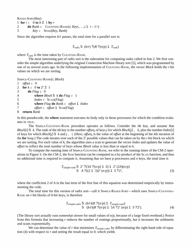
Figure 7 breaks down the running time of radix sort as a function of r for n/p 5 4096. As can be seen from the fig-ure, as r increases, the send time diminishes and the scan time grows. We can determine the value for r that mini-mizes the total time of the algorithm by differentiating the right-hand side of equation (5) with respect to r and set-ting the result equal to 0. For large numbers of keys per processor, the value for r that we obtain satisfies

(n/p)R}}(n/p)5A 1 S

r 5 lg((n/p)(R 1 10A)/(S 1 2A)) 2 lg(r ln 2 2 1) (6)< lg(n/p) 2 lg lg(n/p) 1 1.5. (7)

For n/p 5 4096, as in Figure 7, equation (7) suggests that we set r < 10, which indeed comes very close to mini-mizing the total running time. The marginally better value of r 5 11 can be obtained by solving equation (6)numerically.

Unlike the choice of r dictated by the analysis of SIMPLE-RADIX-SORT, the optimal choice of r for RADIX-SORT grows with n/p. Consequently, for large number of keys per processor, the number of passes of RADIX-SORT

is smaller than that of SIMPLE-RADIX-SORT. When we substitute our choice of r back into equation (5), we obtain

Tradix < (n/p)1 21R 1 10A 1 (S 1 2A)2. (8)

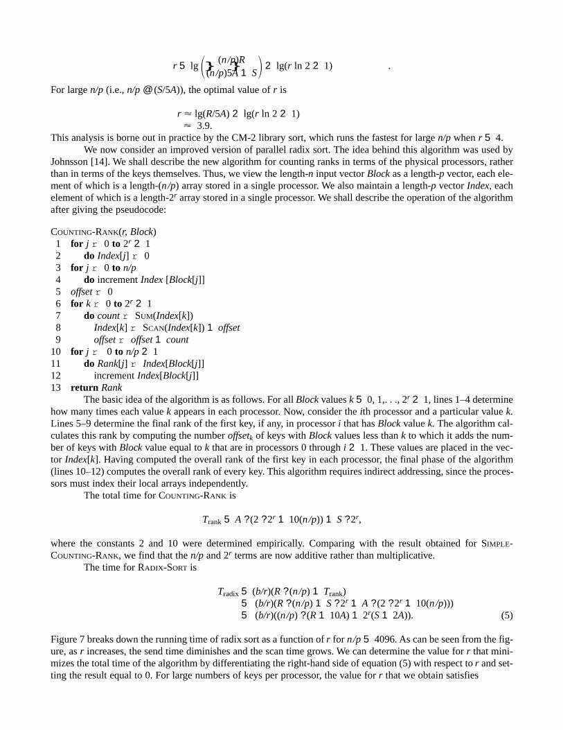
In our implementation of RADIX-SORT, the optimal values of r have been determined empirically. Figure 8 com-pares the performance predicted by equation (8) with the actual running time of our implementation.

Sample SortThe third sort that we implemented is a sample sort [10, 13, 19, 20, 24]. This sorting algorithm was the fastest forlarge sets of input keys, beating radix sort by more than a factor of 2. It also was the most complicated to imple-ment. The sort is a randomized sort: it uses a random number generator. The running time is almost independentof the input distribution of keys and, with very high probability, the algorithm runs quickly.

Assuming n input keys are to be sorted on a machine with p processors, the algorithm proceeds in threephases:1. A set of p 2 1 “splitter” keys are picked that partition the linear order of key values into p “buckets.”2. Based on their values, the keys are sent to the appropriate bucket, where the ith bucket is stored in the ith proces-

sor.3. The keys are sorted within each bucket.If necessary, a fourth phase can be added to load balance the keys, since the buckets do not typically have exactlyequal size.

3}lg(n/p)

b}}}

lg(n/p) 2 lg lg(n/p) 1

Figure 7. A breakdown of the total running time of radix sort into send time and scan time for sorting 64-bit keys(b 5 64) with n/p 5 4096. The total running time is indicated by the top curve. The two shaded areas representthe scan time and send time. As r is increased, the scan time increases and the send time decreases. (The arithmetictime is negligible.) For the parameters chosen, the optimal value of r is 11.

Sample sort gets its name from the way the p 2 1 splitters are selected in the first phase. From the n inputkeys, a sample of ps # n keys are chosen at random, where s is a parameter called the oversampling ratio. Thissample is sorted, and then the p 2 1 splitters are selected by taking those keys in the sample that have ranks s, 2s,3s, . . ., (p 2 1)s.

Some sample sort algorithms [10, 20, 24] choose an oversampling ratio of s 5 1, but this choice results ina relatively large deviation in the bucket sizes. By choosing a larger value, as suggested by Reif and Valiant [19]and by Huang and Chow [13], we can guarantee with high probability that no bucket contains many more keysthan the average. (The Reif-Valiant flashsort algorithm differs in that it uses buckets corresponding to O(lg7 p)-processor subcubes of the hypercube.)

The time for Phase 3 of the algorithm depends on the maximum number, call it L, of keys in a single buck-et. Since the average bucket size is n/p, the efficiency by which a given oversampling ratio s maintains small buck-et sizes can be measured as the ratio L/(n/p), which will be referred to as the bucket expansion. The bucket expan-sion gives the ratio of the maximum bucket size to the average bucket size. The expected value of the bucket expan-sion depends on the oversampling ratio s and on the total number n of keys, and will be denoted by b(s, n).

It is extremely unlikely that the bucket expansion will be significantly greater than its expected value. Ifthe oversampling ratio is s, then the probability that the bucket expansion is greater than some factor a . 1 is

Pr[b(s, n) . a] # ne2(121/a)2as/2. (9)

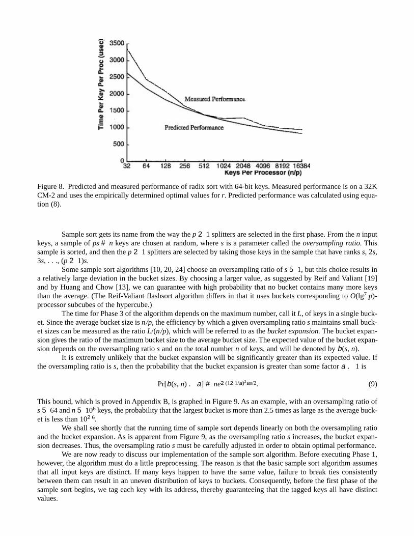
This bound, which is proved in Appendix B, is graphed in Figure 9. As an example, with an oversampling ratio ofs 5 64 and n 5 106 keys, the probability that the largest bucket is more than 2.5 times as large as the average buck-et is less than 1026.

We shall see shortly that the running time of sample sort depends linearly on both the oversampling ratioand the bucket expansion. As is apparent from Figure 9, as the oversampling ratio s increases, the bucket expan-sion decreases. Thus, the oversampling ratio s must be carefully adjusted in order to obtain optimal performance.

We are now ready to discuss our implementation of the sample sort algorithm. Before executing Phase 1,however, the algorithm must do a little preprocessing. The reason is that the basic sample sort algorithm assumesthat all input keys are distinct. If many keys happen to have the same value, failure to break ties consistentlybetween them can result in an uneven distribution of keys to buckets. Consequently, before the first phase of thesample sort begins, we tag each key with its address, thereby guaranteeing that the tagged keys all have distinctvalues.

Figure 8. Predicted and measured performance of radix sort with 64-bit keys. Measured performance is on a 32KCM-2 and uses the empirically determined optimal values for r. Predicted performance was calculated using equa-tion (8).

Phase 1: Selecting the splittersThe first phase of sample sort begins with each processor randomly selecting a set of s tagged keys from amongthose stored in its local memory. We implement this method by partitioning each processor’s n/p keys into s blocksof n/ps keys, and then we choose one key at random from each block. This selection process differs from thatwhere each processor selects s tagged keys randomly from the entire set, as is done in both the Reif-Valiant [19]and Huang-Chow [13] algorithms. All of these methods yield small bucket expansions. Since the CM-2 is a dis-tributed-memory machine, however, the local-choice method has an advantage in performance over global-choicemethods: no global communication is required to select the candidates. In our implementation, we typically picks 5 32 or s 5 64, depending on the number of keys per processor in the input.

Once the sample of tagged keys has been determined, the keys in it are sorted across the machine usingthe simple version of radix sort described in Section 4. (Since radix sort is stable, the tags need not be sorted.) Sincethe sample contains many fewer keys than does the input, this step runs significantly faster than sorting all of thekeys with radix sort. The splitters are now chosen as these tagged keys with ranks s, 2s, 3s, . . ., (p 2 1)s. The actu-al extraction of the splitters from the sample is implemented as part of Phase 2.

The dominant time required by Phase 1 is the time for sorting the candidates:

Tcandidates 5 RS(ps, p), (10)

where RS(ps, p) is the time required to radix sort ps keys on p processors. Using the radix sort from the originalCM-2 PARIS library, we have Tcandidates < 7000A ? s.

Notice that the time for Phase 1 is independent of the total number n of keys, since during the selectionprocess, a processor need not look at all of its n/p keys in order to randomly select from them. Notice also that ifwe had implemented a global-choice sampling strategy, we would have had a term containing R ? s in the expres-sion.

Phase 2: Distributing the keys to bucketsExcept for our local-choice method of picking a sample and the choice of algorithm used to sort the oversampledkeys, Phase 1 follows both the Reif-Valiant and Huang-Chow algorithms. In phase 2, however, we follow Huang-Chow more closely.

Figure 9. Bucket expansion for sampling sorting n 5 106 keys, as a function of oversampling ratio s (p 5 1024).The dashed curves are theoretical upper bounds given by inequality (9) when setting the probability of being with-in the bound to 1 2 1023 (the lower dashed curve) and 1 2 1026 (the upper dashed curve). The solid curves areexperimental values for bucket expansion. The upper solid curve shows the maximum bucket expansion found over103 trials, and the lower solid curve shows the average bucket expansion over 103 trials. In practice, oversamplingratios of s 5 32 or s 5 64 yield bucket expansions of less than 2.

Each key can determine the bucket to which it belongs by performing a binary search of the sorted arrayof splitters. We implemented this part of the phase in a straightforward fashion: the front end reads the splitters oneby one and broadcasts them to each processor. Then, each processor determines the bucket for each of its keys byperforming a binary search of the array of splitters stored separately in each processor. Once we have determinedto which bucket a key belongs, we throw away the tagging information used to make each key unique and routethe keys directly to their appropriate buckets. We allocate enough memory for the buckets to guarantee a very highprobability of accommodating the maximum bucket size. In the unlikely event of a bucket overflow, excess keysare discarded during the route and the algorithm is restarted with a new random seed.

The time required by Phase 2 can be separated into the time for the broadcast, the time for the binarysearch, and the time for the send:

Tbroadcast 5 50A ? p,Tbin-search 5 6.5A ? (n/p) lg p,

Tsend 5 R ? (n/p);

where the constants 50 and 6.5 were determined empirically by instrumenting the code.As is evident by our description and also by inspection of the formula for Tbroadcast, the reading and broad-

casting of splitters by the front end is a serial bottleneck for the algorithm. Our sample sort is really only a rea-sonable sort when n/p is large, however. In particular, the costs due to binary search outweigh the costs due to read-ing and broadcasting the splitters when 6.5(n/p) lg p . 50p, or equivalently, when n/p . (50/6.5)p/lg p. For a 64KCM-2, we have p 5 2048, and the preceding inequality holds when the number n/p of input keys per processor isat least 1432. This number is not particularly large, since each processor on the CM-2 has a full megabyte of mem-ory even when the machine is configured with only 1-megabit DRAM’s.

Phase 3: Sorting keys within processorsThe third phase sorts the keys locally within each bucket. The time taken by this phase is equal to the time takenby the processor with the most keys in its bucket. If the expected bucket expansion is b(s, n), the largest bucket hasexpected size (n/p)b(s, n).

We use a standard serial radix sort in which each pass is implemented using several passes of a countingsort (see, for example, [7, Section 9.3]). Radix sort was used, since it is significantly faster than comparison sortssuch as quicksort. The serial radix sort requires time

Tlocal-sort 5 (b/r)A ? ((1.3)2r 1 10(n/p)b(s, n)), (11)

where b is the number of bits in a key and 2r is the radix of the sort. The first term in the coefficient of A corre-sponds to the b/r (serial) scan computations on a histogram of key values, and the second term corresponds to thework needed to put the keys in their final destinations.

We can determine the value of r that minimizes Tlocal-sort by differentiating the right-hand side of equation(11) with respect to r and setting the result equal to 0. This yields r < lg(n/p) 2 1 for large n/p. With this selec-tion of r, the cost of the first term in the equation is small relative to the second term. Typically, b/r < 6, and b(s,n) < 2, which yields

Tlocal-sort < A ? 10 ? 6(n/p) ? 25 120A ? (n/p). (12)

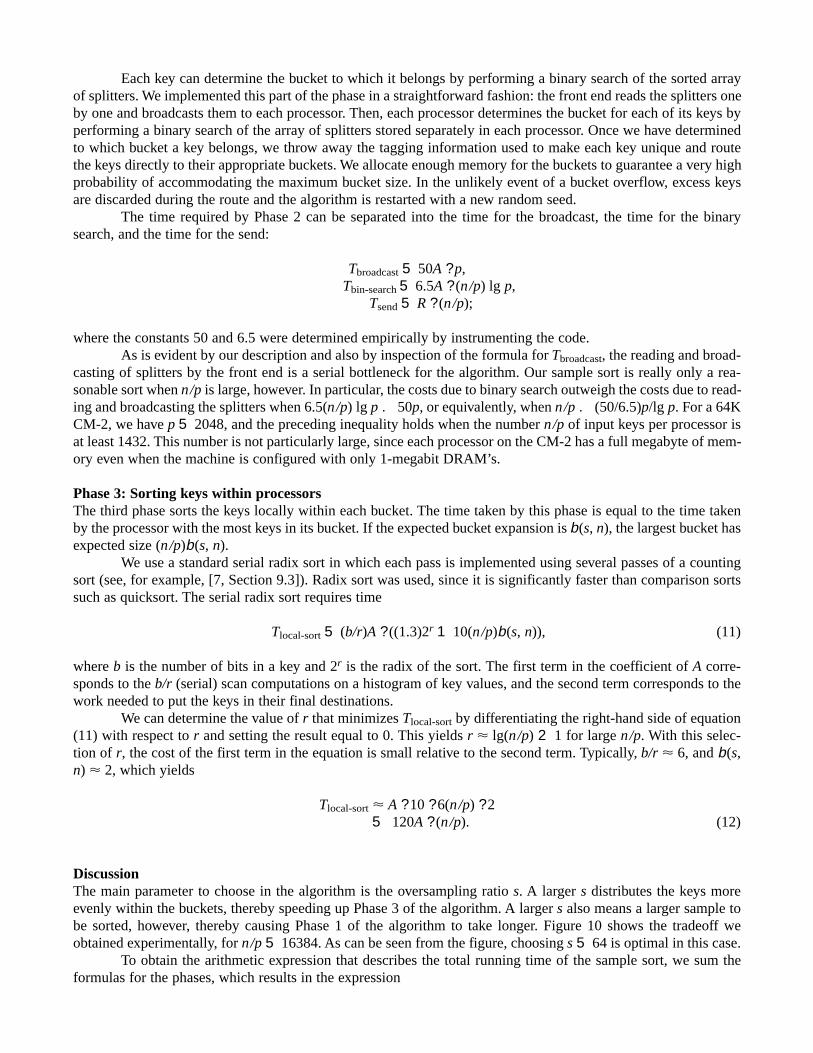
DiscussionThe main parameter to choose in the algorithm is the oversampling ratio s. A larger s distributes the keys moreevenly within the buckets, thereby speeding up Phase 3 of the algorithm. A larger s also means a larger sample tobe sorted, however, thereby causing Phase 1 of the algorithm to take longer. Figure 10 shows the tradeoff weobtained experimentally, for n/p 5 16384. As can be seen from the figure, choosing s 5 64 is optimal in this case.

To obtain the arithmetic expression that describes the total running time of the sample sort, we sum theformulas for the phases, which results in the expression

Tsample 5 Tcandidates 1 Tbroadcast 1 Tbin-search 1 Tsend 1 Tlocal-sort

< 7000A ? s 1 50A ? p 1 6.5A ? (n/p) lg p 1 R ? (n/p) 1 120A ? (n/p),

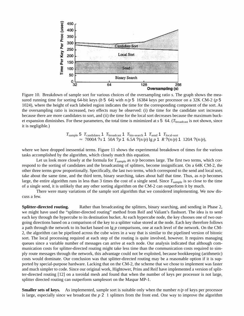
where we have dropped inessential terms. Figure 11 shows the experimental breakdown of times for the varioustasks accomplished by the algorithm, which closely match this equation.

Let us look more closely at the formula for Tsample as n/p becomes large. The first two terms, which cor-respond to the sorting of candidates and the broadcasting of splitters, become insignificant. On a 64K CM-2, theother three terms grow proportionally. Specifically, the last two terms, which correspond to the send and local sort,take about the same time, and the third term, binary searching, takes about half that time. Thus, as n/p becomeslarge, the entire algorithm runs in less than 3 times the cost of a single send. Since Tsample is so close to the timeof a single send, it is unlikely that any other sorting algorithm on the CM-2 can outperform it by much.

There were many variations of the sample sort algorithm that we considered implementing. We now dis-cuss a few.

Splitter-directed routing. Rather than broadcasting the splitters, binary searching, and sending in Phase 2,we might have used the “splitter-directed routing” method from Reif and Valiant’s flashsort. The idea is to sendeach key through the hypercube to its destination bucket. At each hypercube node, the key chooses one of two out-going directions based on a comparison of the key to a splitter value stored at the node. Each key therefore followsa path through the network to its bucket based on lg p comparisons, one at each level of the network. On the CM-2, the algorithm can be pipelined across the cube wires in a way that is similar to the pipelined version of bitonicsort. The local processing required at each step of the routing is quite involved, however. It requires managingqueues since a variable number of messages can arrive at each node. Our analysis indicated that although com-munication costs for splitter-directed routing might take less time than the communication costs required to sim-ply route messages through the network, this advantage could not be exploited, because bookkeeping (arithmetic)costs would dominate. Our conclusion was that splitter-directed routing may be a reasonable option if it is sup-ported by special-purpose hardware. Lacking that on the CM-2, the scheme that we chose to implement was fasterand much simpler to code. Since our original work, Hightower, Prins and Reif have implemented a version of split-ter-directed routing [12] on a toroidal mesh and found that when the number of keys per processor is not large,splitter directed routing can outperform samplesort on the Maspar MP-1.

Smaller sets of keys. As implemented, sample sort is suitable only when the number n/p of keys per processoris large, especially since we broadcast the p 2 1 splitters from the front end. One way to improve the algorithm

Figure 10. Breakdown of sample sort for various choices of the oversampling ratio s. The graph shows the mea-sured running time for sorting 64-bit keys (b 5 64) with n/p 5 16384 keys per processor on a 32K CM-2 (p 51024), where the height of each labeled region indicates the time for the corresponding component of the sort. Asthe oversampling ratio is increased, two effects may be observed: (i) the time for the candidate sort increasesbecause there are more candidates to sort, and (ii) the time for the local sort decreases because the maximum buck-et expansion diminishes. For these parameters, the total time is minimized at s 5 64. (Tbroadcast is not shown, sinceit is negligible.)

when each processor contains relatively few input keys would be to execute two passes of phases 1 and 2. In thefirst pass, we can generate Ïpw 2 1 splitters and assign a group of Ïpw processors to each bucket. Each key canthen be sent to a random processor within the processor group corresponding to its bucket. In the second pass, eachgroup generates Ïpw splitters which are locally broadcast within the subcubes, and then keys are sent to their finaldestinations. With this algorithm, many fewer splitters need to be distributed to each processor, but twice the num-ber of sends are required. This variation was not implemented, because we felt that it would not outperform biton-ic sort for small values of n/p.

Load balancing. When the three phases of the algorithm are complete, not all processors have the samenumber of keys. Although some applications of sorting—such as implementing a combining send or heuristic clus-tering—do not require that the processor loads be exactly balanced, many do. Load balancing can be performed byfirst scanning to determine the destination of each sorted key and then routing the keys to their final destinations.The dominant cost in load balancing is the extra send. We implemented a version of sample sort with load bal-ancing. With large numbers of keys per processor, the additional cost was only 30 percent, and the algorithm stilloutperforms the other sorts.

Key distribution. The randomized sample sort algorithm is insensitive to the distribution of keys, but unfor-tunately, the CM-2 message router is not, as mentioned earlier. In fact, for certain patterns, routing can take up totwo and a half times longer than normally expected. This difficulty can be overcome, however, by randomizing thelocation of buckets. For algorithms that require the output keys in the canonical order of processors, an extra sendis required, as well as a small amount of additional routing so that the scan for load balancing is performed in thecanonical order. This same send can also be used for load balancing.

Figure 11. A breakdown of the actual running time of sample sort, as a function of the input size n. The graphshows actual running times for 64-bit keys on a 32K CM-2 (p 5 1024). The per-key cost of broadcasting splittersdecreases as n/p increases, since the total cost of the broadcast is independent of n. The per-key cost of the candi-date sort decreases until there are 4K keys per processor; at this point, we increase the oversampling ratio from s 532 to s 5 64 in order to reduce the time for local sorting. The local sort improves slightly at higher values of n/p,because the bucket expansion decreases while the per-key times for send and binary search remain constant.

ConculsionsOur goal in this project was to develop a system sort of the Connection Machine. Because of this goal, raw speedwas not our only concern. Other issues included space, stability, portability, and simplicity. Radix sort has sever-al notable advantages with respect to these criteria. Radix sort is stable, easy to code and maintain, performs rea-sonably well over the entire range of n/p, requires less memory than sample sort, and performs well on short keys.Although the other two sorts have domains of applicability, we concluded that the radix sort was most suitable as

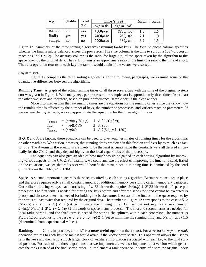
a system sort.Figure 12 compares the three sorting algorithms. In the following paragraphs, we examine some of the

quantitative differences between the algorithms.

Running Time. A graph of the actual running times of all three sorts along with the time of the original systemsort was given in Figure 1. With many keys per processor, the sample sort is approximately three times faster thanthe other two sorts and therefore, based on pure performance, sample sort is the clear winner.

More informative than the raw running times are the equations for the running times, since they show howthe running time is affected by the number of keys, the number of processors, and various machine parameters. Ifwe assume that n/p is large, we can approximate the equations for the three algorithms as

Tbitonic < (n/p)(Q ? (lg p) 1 A ? 2.5(lg2 n))Tradix < (n/p)(R ? 6 1 A ? 80)Tsample < (n/p)(R 1 A ? (5 lg p 1 120)).

If Q, R and A are known, these equations can be used to give rough estimates of running times for the algorithmson other machines. We caution, however, that running times predicted in this fashion could err by as much as a fac-tor of 2. The A terms in the equations are likely to be the least accurate since the constants were all derived empir-ically for the CM-2, and they depend highly on the local capabilities of the processors.

The equations can also give an idea of how much would be gained in each sorting algorithm by improv-ing various aspects of the CM-2. For example, we could analyze the effect of improving the time for a send. Basedon the equations, we see that radix sort would benefit the most, since its running time is dominated by the send(currently on the CM-2, R 5 130A).

Space. A second important concern is the space required by each sorting algorithm. Bitonic sort executes in placeand therefore requires only a small constant amount of additional memory for storing certain temporary variables.Our radix sort, using n keys, each consisting of w 32-bit words, requires 2w(n/p) 1 2r 32-bit words of space perprocessor. The first term is needed for storing the keys before and after the send (the send cannot be executed inplace), and the second term is needed for holding the bucket sums. Because of the first term, the space required bythe sort is at least twice that required by the original data. The number in Figure 12 corresponds to the case w 5 2(64-bits) and r 5 lg(n/p) 2 2 (set to minimize the running time). Our sample sort requires a maximum of2w(n/p)b(s, n) 1 2r 1 (w 1 1)p 32-bit words of space in any processor. The first and second terms are needed forlocal radix sorting, and the third term is needed for storing the splitters within each processor. The number inFigure 12 corresponds to the case w 5 2, r 5 lg(n/p) 2 1 (set to minimize the running time) and b(s, n) {app} 1.5(determined from experimental values).

Ranking. Often, in practice, a “rank” is a more useful operation than a sort. For a vector of keys, the rankoperation returns to each key the rank it would attain if the vector were sorted. This operation allows the user torank the keys and then send a much larger block of auxiliary information associated with each key to the final sort-ed position. For each of the three algorithms that we implemented, we also implemented a version which gener-ates the ranks instead of the final sorted order. To implement a rank operation in terms of a sort, the original index

Figure 12. Summary of the three sorting algorithms assuming 64-bit keys. The load balanced column specifieswhether the final result is balanced across the processors. The time column is the time to sort on a 1024-processormachine (32K CM-2). The memory column is the ratio, for large n/p, of the space taken by the algorithm to thespace taken by the original data. The rank column is an approximate ratio of the time of a rank to the time of a sort.The rank operation returns to each key the rank it would attain if the vector were sorted.

in the vector is tagged onto each key and is then carried around during the sort. Once sorted, the final index is sentback to the location specified by the tag (the key’s original position). In a radix-sort-based implementation of therank operation, the cost of the additional send can be avoided by omitting the last send of radix sort, and sendingthe rank directly back to the index specified by the tag. Furthermore, as each block of the key is used by radix sort,that block can be thrown away, thereby shortening the message length of subsequent sends. Because of this, thetime of “radix-rank” is only marginally more expensive than that of radix sort. For sample sort and bitonic sort,carrying the tag around slows down the algorithm by a factor of between 1.3 and 1.5.

Stability. Radix sort is stable, but the other two sorts are not. Bitonic sort and sample sort can be made sta-ble by tagging each key with its initial index, as is done for the rank. In this case, however, not only must the tagbe carried around during the sends, it must also be used in the comparisons. Sorting the extra tag can cause a slow-down of up to a factor of 1.5.

Key Length. Another issue is sorting short keys—keys with perhaps 10, 16, or 24 significant bits. Sorting shortkeys is a problem that arises reasonably often in CM-2 applications. For short keys, the time required by bitonicsort is not at all improved over the 32-bit time. The time required by the sample sort is marginally improved, sincethe cost of the local radix sort is reduced. The time required by radix sort, however, is essentially proportional tothe key length. Since r is typically in the range 10 # r , 16, sorting 20 bits requires 2 passes instead of 3 to 4 for32 bits and 5 to 7 for 64 bits.

Appendix A. Other Sorts of SortsMany algorithms have been developed for sorting on the hypercube and related networks such as the butterfly,cube-connected cycles, and shuffle-exchange. We considered a number of these algorithms before deciding toimplement bitonic sort, radix sort, and sample sort. The purpose of this section is to discuss some of the other sort-ing algorithms considered and, in particular, to indicate why these alternatives were not selected for implementa-tion.

Quicksort. It is relatively easy to implement a parallel version of quicksort on the CM-2 using segmentedscans. First, a pivot is chosen at random and broadcast using scans. The pivot partitions the keys into small keysand large keys. Next, using scans, each small key is labeled with the number of small keys that precede it in thelinear order, and each large key is labeled with the number of large keys that precede it, plus the total number ofsmall keys. The keys are then routed to the locations specified by their labels. The new linear order is broken intotwo segments, the small keys and the large keys, and the algorithm is recursively applied to each segment. Theexpected number of levels of recursion is close to lg n, and, at each level, the algorithm performs 1 route andapproximately 7 scans. This algorithm has been implemented in a high level language (*Lisp) and runs about 2times slower than the original system sort. We believed that we could not speed it up significantly, since the scanand route operations are already performed in hardware.

Hyperquicksort. The hyperquicksort algorithm [23] can be outlined as follows. First, each hypercube nodesorts its n/p keys locally. Then, one of the hypercube nodes broadcasts its median key, m, to all of the other nodes.This key is used as a pivot. Each node partitions its keys into those smaller than m, and those larger. Next, thehypercube nodes exchange keys along the dimension-0 edges of the hypercube. A node whose address begins with0 sends all of its keys that are larger than m to its neighbor whose address begins with 1. The neighbor sends backall of its keys that are smaller than m. As keys arrive at a node, they are merged into the sorted sequence of keysthat were not sent by that node. Finally, the algorithm is recursively applied to the p/2-node subcubes whoseaddresses begin with 0 and 1, respectively.

The communication cost of hyperquicksort is comparable to that of the fully-pipelined version of bitonicsort. The expected cost is at least Q n lg p/2p since the algorithm uses the lg p dimensions one at a time and, foreach dimension, every node expects to send half of its n/p keys to its neighbor. The cost of bitonic sort is alwaysQ ? (lg p)(n/p 1 (lg p)/2 2 1/2).

The main advantage of bitonic sort over hyperquicksort is that its performance is not affected by the ini-tial distribution of the keys to be sorted. Hyperquicksort relies on a random initial distribution to ensure that the

Sparse enumeration sort. The Nassimi-Sahni sorting algorithm [17], which will be referred to as space enu-meration sort, is used when the number n of items to be sorted is smaller than the number p of processors. In thespecial case n 5 p, sparse enumeration sort is a very simple algorithm indeed. The n records are initially storedone-per-processor in the n lowest-numbered processors; viewing the processors of the hypercube as forming a two-dimensional n 3 n array, the input records occupy the first row of the array. Sparse enumeration sort proceeds byperforming a set of n parallel column broadcasts (from the topmost entry in each column) followed by n parallelrow broadcasts (from the diagonal positions), so that the processor at row i and column j of the array contains acopy of the ith and jth items. At this point, all pairs of items can be simultaneously compared in constant time, andprefix operations over the rows can be used to compute the overall rank of each item. The ith row is then used toroute a copy of item i to the column corresponding to its output rank. Finally, a set of n parallel routes is used tomove each item to its sorted output position in the first row. For values of n strictly less than Ïpw, sparse enumer-ation sort proceeds in exactly the same fashion: n2 processors are used, and the remaining p 2 n2 processors areidle. Thus, sparse enumeration sort runs in O(lg n) time when n # Ïpw.

Sparse enumeration sort generalizes the preceding algorithm in an elegant manner to obtain a smoothtradeoff between O(lg n) performance at n 5 Ïpw and O(lg2 n) performance at n 5 p (the performance of bitonicsort). In this range, sparse enumeration sort is structured as a (p/n)-way merge sort. After the ith set of parallelmerges, the n items are organized into n(n/p)i sorted lists of length (p/n)i. The ith set of merges is performed in O(ilg(p/n)) time using a constant number of bitonic merges, prefix operations, and monotone routes. Monotone routesare a special class of routing operations that can be performed deterministically, on-line in a collision-free manner.On the CM-2, monotone routes would be implemented using cube swaps; the entire implementation of sparse enu-meration sort would not make use of the CM-2 router. A straightforward computation shows that the overall timecomplexity of sparse enumeration sort is O(lg2 n/lg(p/n)) time.

For sufficiently large values of the ratio p/n . 1, one would expect sparse enumeration sort would performbetter than the other sorts we looked at. It is unclear, however, that one would need a parallel computer to solvesuch small problems and one might get better times by solving the problem on a single processor, or by reducingp.

Column sort. Column sort [15] is an elegant parallel sorting technique that has found many theoretical applica-tions. Column sorts n keys using two primitive operations. The first primitive operation is to sort n1/3 separate sets(called columns) of n2/3 keys each. Depending on the particular application, this sorting primitive may either beaccomplished by a recursive call or, more typically, by some other sorting algorithm. The second primitive opera-tion is to route all n keys according to a fixed permutation. Alternating between sorts and routes 4 times sufficesto sort all n elements.

If n $ p3, then column sort runs quite efficiently. The sorting primitive is executed as a local sort, and allof the fixed permutations required by column sort are straightforward to implement in a greedy, collision-free man-ner. In terms of the CM-2, they can be implemented with a simple sequence of cube swaps rather than by involv-ing the router. As another implementation optimization, we remark that the “standard” column sort algorithm isnot pipelined and would only make use of a 1 / lg p fraction of the CM-2 wires at any given time. A U(lg p) speedupcan be achieved by pipelining, and there are at least two approaches worthy of consideration. The first approach isto partition the data at each processor into lg p equal-sized sets, interleave lg p column sorts, and then merge theresulting lg p sorted lists. The second approach is to pipeline each of the routing operations in a single applicationof column sort.

The main drawback of column sort is that, for n , p3, some degree (depending on the ratio n/p) of recur-sion is necessary in order to perform the sorting primitive; sets of n2/3 items occupy more than a single processor.We chose not to implement column sort because it appeared that the condition n $ p3 would not be satisfied inmany cases of interest, and a close analysis of critical sections of the potential code indicated that a recursive ver-sion of column sort would provide little, if any, improvement over either radix sort or sample sort. Furthermore,the relative performance of column sort would tend to degrade quite severely for small values of the ratio n/p.

The asymptotic performance of column sort is best understood by considering arithmetic and communi-cation costs separately. Let us assume that n $ p11e, where e denotes an arbitrary positive constant, which implies

work each processor has to do is reasonably balanced. Although hyperquicksort may perform less arithmetic thanbitonic sort in the best case, it uses indirect addressing, which is relatively expensive on the CM-2.

a bounded depth of recursion. Under this assumption, the total arithmetic cost of column sort is U((n/p) lg n),which is optimal for any comparison-based sort. With pipelining, the communication cost of column sort is U(n/p),which is optimal for any sorting algorithm.

To summarize, although we felt that column sort might turn out to be competitive at unusually high loads(n $ p3), its mediocre performance at high loads (p2 # n , p3), and poor performance at low to moderate loads(p # n , p2) made other alternatives more attractive. Column sort might well be a useful component of a hybridsorting scheme that automatically selects an appropriate algorithm depending upon the values of n and p.

Cubesort. Like Leighton’s column sort, the cubesort algorithm of Cypher and Sanz [9] gives a scheme forsorting n items in a number of “rounds”, where in each round the data is partitioned into n/s sets of size s (for somes, 2 # s # n), and each set is sorted. (Successive partitions of the data are determined by simple fixed permuta-tions that can be routed just as efficiently as those used by column sort.) The main advantage of cubesort over col-umn sort is that, for a wide range of values of s, cubesort requires asymptotically fewer rounds than column sort.In particular, for 2 # s # n, column sort (applied recursively) uses U((lg n/lg s)b) rounds for b 5 2/(lg 3 2 1) <3.419, whereas cubesort uses only O((25)lg* n- lg* s(lg n/lg s)2) rounds. (The cost of implementing a round is essen-tially the same in each case.) For n $ p3, cubesort can be implemented without recursion, but requires 7 rounds asopposed to 4 for column sort. For n , p3, both cubesort and column sort are applied recursively. For n sufficient-ly smaller than p3 (and p sufficiently large), the aforementioned asymptotic bounds imply that cubesort will even-tually outperform column sort. However, for practical values of n and p, if such a crossover in performance everoccurs, it appears likely to occur at a point where both cubesort and column sort have poor performance relativeto other algorithms (e.g., at low to moderate loads).

Nonadaptive smoothsort. There are several variants of the smoothsort algorithm, all of which are describedin [18]. The most practical variant, and the one of interest to us here, is the nonadaptive version of smoothsort algo-rithm. The structure of this algorithm, hereinafter referred to simply as “smoothsort,” is similar to that of columnsort. Both algorithms make progress by ensuring that under a certain partitioning of the data into subcubes, the dis-tribution of ranks of the items within each subcube is similar. The benefit of performing such a “balancing” oper-ation is that after the subcubes have been recursively sorted, all of the items can immediately be routed close totheir correct position in the final sorted order (i.e., the subcubes can be approximately merged in an oblivious fash-ion). The effectiveness of the algorithm is determined by how close (in terms of number of processors) every itemis guaranteed to come to its correct sorted position. It turns out that for both column sort as well as smoothsort, theamount of error decreases as n/p, the load per processor, is increased.

As noted in the preceding section, for n $ p3, column sort can be applied without recursion. This is due tothe fact that after merging the balanced subcubes, every item has either been routed to the correct processor i, orit has been routed to one of processors i 2 1 and i 1 1. Thus, the sort can be completed by performing local sortsfollowed by merge-and-split operations between odd and even pairs of adjacent processors. As a simple optimiza-tion, it is more efficient to sort the ith largest set of n/p items to the processor with the ith largest standard Graycode instead of processor i. This permits the merge-and-split operations to be performed between adjacent proces-sors.

The main difference between column sort and smoothsort is that the “balancing” operation performed bysmoothsort (the cost of which is related to that of column sort by a small constant factor) guarantees as asymptot-ically smaller degree of error. For this reason, smoothsort can be applied without recursion over a larger range ofvalues of n and p, namely, for n $ p2 lg p. Interestingly, the balancing operation of smoothsort is based upon a sim-ple variant of merge-and-split: the “merge-and-unshuffle” operation. Essentially, the best way to guarantee simi-larity between the distribution of ranks of the items at a given pair A and B of adjacent processors is to merge thetwo sets of items, assign the odd-ranked items in the resulting sorted list to processor A (say), and the even-rankeditems to processor B. This effect is precisely that of a merge-and-unshuffle operation. The balancing operation ofsmoothsort amounts to performing lg p sets of such merge-and-unshuffle operations, one over each of the hyper-cube dimensions. As in the case of column sort, there are at least two ways to pipeline the balancing operation inorder to take advantage of the CM-2’s ability to communicate across all of the hypercube wires at once.

At high loads (p2 # n , p3), we felt that smoothsort might turn out to be competitive with sample-sort.Like column sort, however, the performance of smoothsort degrades (relative to that of other algorithms) at low to

moderate loads (p # n , p2), which was the overriding factor in our decision not to implement smoothsort. Forunusually high loads (n $ p3), it is likely that column sort would slightly outperform smoothsort because of a smallconstant factor advantage in the running time of its balancing operation on the CM-2. It should be mentioned thatfor n $ p11e, the asymptotic performance of smoothsort is the same as that of column sort, both in terms of arith-metic as well as communication. Smoothsort outperforms column sort for smaller values of n/p, however. For adetailed analysis of the running time of smoothsort, the reader is referred to [18].

Theoretical results. This subsection summarizes several “theoretical” sorting results—algorithms with opti-mal or near-optimal asymptotic performance but which remain impractical due to large constant factors and/ornonconstant costs that are not accounted for by the model of computation. In certain instances, a significant addi-tional penalty must be paid in order to “port” the algorithm to the particular architecture provided by the CM-2.

Many algorithms have been developed for sorting on Parallel Random Access Machines (PRAMs). Thefastest comparison-based sort is Cole’s parallel merge sort [6]. This algorithm requires optimal O(lg n) time to sortn items on an n-node exclusive-read exclusive-write (EREW) PRAM. Another way to sort in O(lg n) time is toemulate the AKS sorting circuit [1]. The constants hidden by the O-notation are large, however.

If one is interested in emulating a PRAM algorithm on a fixed interconnection network such as the hyper-cube or butterfly, the cost of the emulation must be taken into account. Since emulation schemes tend to be basedon routing, and the cost of routing seems to be intimately related to that of sorting, it is perhaps unlikely that anysorting algorithm developed for the PRAM model will lead to an optimal solution in the fixed interconnection net-work model.

For the hypercube and related networks such as the butterfly, cube-connected cycles, and shuffle-exchange, there have been recent asymptotic improvements in both the deterministic and randomized settings. Adeterministic, O(lg n(lg lg n)2)-time algorithm for the case n 5 p is described in [8]. An O(lg n)-time algorithmthat admits an efficient bit-serial implementation and also improves upon the asymptotic failure probability of theReif-Valiant flashsort algorithm is presented in [16]. Unfortunately, both of these algorithms are quite impractical.The reader interested in theoretical bounds should consult the aforementioned papers for further references to pre-vious work.

Appendix B. Probabilistic Analysis of Sample SortThis appendix analyzes the sizes of the buckets created by the sample sort algorithm. Recall how buckets are cre-ated, a method we’ll call Method P. First, each of the p processors partitions its n/p keys into s groups of n/ps andselects one candidate at random from each group. Thus, there are a total of exactly ps candidates. Next, the candi-dates are sorted, and every sth candidate in the sorted order is chosen to be a splitter. The keys lying between twosuccessive splitters form a bucket. Theorem B.4 will show that it is unlikely that this method assigns many morekeys than average to any one bucket.

The proof of Theorem B.4 uses three lemmas, the first two of which are well known in the literature. Thefirst is due to Hoeffding.

Lemma B.1 Let Xi be a random variable that is equal to 1 with probability qi and to 0 with probability 1 2 qi,for i 5 1, 2, . . ., n. Let W 5 Sn

i51 Xi, which implies that E[W] 5 Sni51 qi. Let q 5 E[W]/n, and let Z be the sum of

n random variables, each equal to 1 with probability q and to 0 with probability 1 2 q. (Note that E[W] 5 E[Z] 5qn.) If k # qn 2 1 is an integer, then

Pr[W # k] # Pr[Z # k].

Our second lemma is a “Chernoff” bound due to Angluin and Valiant [11].

Lemma B.2 Consider a sequence of r Bernoulli trials, where success occurs in each trial with probability q.Let Y be the random variable denoting the total number of successes. Then for 0 # g # 1, we have

Pr[Y # grq] # e1 (12g)2rq/2.

Our third lemma shows that Method P can be analyzed in terms of another simpler method we call MethodI. In Method I, each key of the n keys independently chooses to be a candidate with probability ps/n. For thismethod, the expected number of candidates is ps. The following lemma shows that upper bounds for Method Iapply to Method P.

Lemma B.3 Let S be a set of n keys, and let T denote an arbitrary subset of S. Let YP and YI denote the num-ber of candidates chosen from T by Methods P and I, respectively. Then for any integer k # (|T|ps/n) - 1, we have

Pr[YP # k] # Pr[YI # k].

Proof: Let {Si} be the partition of keys used by Method P, that is, S 5 <psi51 Si and |Si| 5 n/ps. Define Ti 5 Si >

T, for i 5 1, 2, . . ., ps. Since |Ti| # |Si| 5 n/ps, each set Ti contributes 1 candidate with probability |Ti|ps/n, and 0candidates otherwise.

Now, define |T| 021 random variables as follows. For each nonempty Ti, define |Ti| random variables,where the first random variable is equal to 1 with probability |Ti|ps/n and 0 otherwise, and the remaining |Ti| 2 1random variables are always 0.

Call the resulting set of |T| random variables X1, . . ., X|T| (order is unimportant), and let YP be the randomvariable defined by YP 5 S

i51 T Xi. Consequently,

E[YP] 5 ^ps

i51|Ti|ps/n 5 |T|ps/n,

and thus, YP is the random variable corresponding to the number of candidates chosen from the set T by MethodP.

Define YI to be the sum of |T| ps/n-biased Bernoulli trials. Note that YI is the random variable correspond-ing to the number of candidates chosen from the set T by Method I. Hence, by substituting W 5 YP and Z 5 YI intoHoeffding’s inequality, we have

Pr[YP # k] # Pr[YI # k]

for k # E[YP] 2 1 5 E[YI] 2 1 5 (|T|ps/n) 2 1. h

With Lemmas B.1 and B.3 in hand, we are prepared to prove the bound given by inequality 9.

Theorem B.4 Let n be the number of keys in a sample sort algorithm, let p be the number of processors, and lets be the oversampling ratio. Then for any a . 1, the probability that Method P causes any bucket to contain morethan an/p keys is at most ne2(121/a)2as/2.

Proof: To prove that no bucket receives more than an/p keys, it suffices to show that the distance l from any keyto the next splitter in the sorted order is at most an/p. We begin by looking at a single key. We have I . an/p onlyif fewer than s of the next an/p keys in the sorted order are candidates. Let T denote this set of an/p keys. Let YP

denote the number of candidates in T, which are chosen according to Method P. Thus, Pr[l . an/p] # Pr[YP , s].We can obtain an upper bound on Pr[YP , s] by analyzing Method I instead of Method P, since by Lemma

B.3, any upper bound derived for Pr[YI # s] also applies to Pr[YP # s], as long as s # (|T|ps/n) 2 1. If the candi-dates are chosen according to Method I, then the number of candidates in the set T of an/p keys has a binomialdistribution, that is,

Pr[YI 5 k] 5 1 2qk(1 2 q)r2k,

where r 5 an/p is the number of independent Bernoulli trials, q 5 ps/n is the probability of success in each trial,and YI is the number of successes. The probability that fewer successes occur than expected can be bounded usingthe “Chernoff” bound

Pr[YI # grq] # e2(12g)2rq/2,

rk

which holds for 0 # g # 1. Substituting r 5 an/p, q 5 ps/n, and g 5 1/a, we have

Pr[l . an/p] # Pr[YP # s]# Pr[YI # s]# e2(121/a)2as/2.

The probability that the distance from any of the n keys to the next splitter is more than an/p is at most thesum of the individual probabilities, each of which is bounded by e1(121/a)2as/2. Since there are are n keys, the prob-ability that the distance from any key to the next splitter is greater than an/p is therefore at most ne2(121/a)2as/2,which proves the theorem.

AcknowledgmentsMany people were involved in this project, and we would like to thank all of them. We would particularly like tothank Mark Bromley, Steve Heller, Bradley Kuszmaul and Kevin Oliveau of Thinking Machines Corporation forhelping with various aspects of the CM-2, including the implementation of the send that was needed for the sam-ple sort. We would also like to thank John Mucci of Thinking Machines and Rita of Rita’s for his support and herinspiration.

References1. M. Ajtai, J. Komlos, and E. Szemeredi. Sorting in c log n parallel steps. Combinatorica, 3:1–19, 1983.2. S. G. Akl. Parallel Sorting Algorithms. Academic Press, Toronto, 1985.3. K. Batcher. Sorting networks and their applications. In Proceedings of the AFIPS Spring Joint Computing

Conference, volume 32, pages 307–314, 1968.4. G. Baudet and D. Stevenson. Optimal sorting algorithms for parallel computers. IEEE Transactions on

Computers, C-27:84–87, 1978.5. G. E. Blelloch. Vector Models for Data-Parallel Computing. The MIT Press, 1990.6. R. Cole. Parallel merge sort. SIAM Journal on Computing, pages 770–785, 1988.7. T. H. Cormen, C. E. Leiserson, and R. L. Rivest. Introduction to Algorithms. The MIT Press and McGraw-

Hill, 1990.8. R. E. Cypher and C. G. Plaxton. Deterministic sorting in nearly logarithmic time on the hypercube and relat-

ed computers. In Proceedings of the 22nd Annual ACM Symposium on Theory of Computing, pages 193–203,May 1990.

9. R. E. Cypher and J. L. C. Sanz. Cubesort: A parallel algorithm for sorting N data items with S-sorters. Journalof Algorithms, 13:211–234, 1992.

10. W. D. Frazer and A. C. McKellar. Samplesort: A sampling approach to minimal storage tree sorting. Journalof the ACM, 17(3):496–507, 1970.

11. T. Hagerup and C. Rub. A guided tour of Chernoff bounds. Information Processing Letters, 33(6):305–308,February 1990.

12. William L. Hightower, Jan F. Prins, and John H. Reif. Implementations of randomized sorting on large paral-lel machines. In Proceedings of the Symposium on Parallel Algorithms and Architectures, June 1992.

13. J. S. Huang and Y. C. Chow. Parallel sorting and data partitioning by sampling. In Proceedings of the IEEEComputer Society’s Seventh International Computer Software and Applications Conference, pages 627–631,November 1983.

14. Lennart Johnsson. Combining parallel and sequential sorting on a boolean n-cube. In Proceedings of theInternational Conference on Parallel Processing, pages 444–448, 1984.

15. F. T. Leighton. Tight bounds on the complexity of parallel sorting. IEEE Transactions on Computers, C-34(4):344–354, April 1985.

16. T. Leighton and G. Plaxton. A (fairly) simple circuit that (usually) sorts. In Proceedings of the 31st AnnualSymposium on Foundations of Computer Science, pages 264–274, October 1990.

17. D. Nassimi and S. Sahni. Parallel permutation and sorting algorithms and a new generalized connection net-work. Journal of the ACM, 29(3):642–667, July 1982.

18. C. G. Plaxton. Efficient computation on sparse interconnection networks. Technical Report STAN-CS-89-

1283, Stanford University, Department of Computer Science, September 1989.19. J. H. Reif and L. G. Valiant. A logarithmic time sort for linear size networks. Journal of the ACM, 34(1):60–76,

January 1987.20. S. R. Seidel and W. L. George. Binsorting on hypercubes with d-port communication. In Proceedings of the

Third Conference on Hypercube Concurrent Computers, pages 1455–1461, January 1988.21. Thomas M. Stricker. Supporting the hypercube programming model on mesh architectures (a fast sorter for

iWarp tori). In Proceedings of the Symposium on Parallel Algorithms and Architectures, June 1992.22. K. Thearling and S. Smith. An improved supercomputer sorting benchmark. In Proceedings Supercomputing

‘92, pages 14–19, November 1992.23. B. A. Wagar. Hyperquicksort: A fast sorting algorithm for hypercubes. In M. T. Heath, editor, Hypercube

Multiprocessors 1987 (Proceedings of the Second Conference on Hypercube Multiprocessors), pages292–299, Philadelphia, PA, 1987. SIAM.

24. Y. Won and S. Sahni. A balanced bin sort for hypercube multicomputers. Journal of Supercomputing,2:435–448, 1988.

25. Marco Zagha and Guy E. Blelloch. Radix sort for vector multiprocessors. In Proceedings Supercomputing ‘91,pages 712–721, November 1991.

This research was supported in part by Thinking Machines Corporation, and in part by the Defense AdvancedResearch Projects Agency under Contracts N00014-87-0825 and F33615-90-C-1465. CM-2, Connection Machine,CM, *Lisp, Paris, and CMIS are trademarks of Thinking Machines Corporation.