A Comparison of Qualitative and Quantitative Firm Performance

Measures

Richard Fabling, Arthur Grimes and Philip Stevens

Ministry of Economic Development

Occasional Paper 08/04

May 2008

ISBN: 978-0-478-31659-9 (PDF) ISBN: 978-0-478-31667-4 (online)

Ministry of Economic Development Occasional Paper 08/04

A Comparison of Qualitative and Quantitative Firm Performance Measures

Date: May 2008

Authors: Richard Fabling (Reserve Bank of New Zealand)

Arthur Grimes (Motu Economic & Public Policy Research)

Philip Stevens (Ministry of Economic Development)

Acknowledgements

The authors gratefully acknowledge the contributions of the members of the

Improved Business Understanding via Longitudinal Database Development (IBULDD)

project. We would like to thank Eileen Basher, Julia Gretton, Hamish Hill, Rodney

Jer, Tas Papadopoulos, Claire Powell and Steve Walshe from Statistics New

Zealand, John Forth, Lynda Sanderson, Steve Stillman, Jason Timmins and

participants at the New Zealand Association of Economists conference in

Christchurch, 2007. We acknowledge funding from the Cross-Departmental

Research Funding in making the IBULDD and hence this work possible.

Contact: Occasionalpapers@med.govt.nz

Disclaimer

Access to the data used in this study was provided by Statistics New Zealand under

conditions designed to give effect to the security and confidentiality provisions of the

Statistics Act 1975. The research was funded by the Ministry of Economic

Development and supported by Statistics New Zealand as part of the Improved

Business Understanding via Longitudinal Database Development project (IBULDD).

The results of this study are based in part on tax data supplied by Inland Revenue to

Statistics New Zealand under the Tax Administration Act. This tax data must be used

only for statistical purposes, and no individual information is provided back to Inland

Revenue for administrative or regulatory purposes. Any discussion of data limitations

or weaknesses is in the context of using the data for statistical purposes, and is not

related to the ability of the data to support Inland Revenue's core operational

requirements. Careful consideration has been given to the privacy, security and

confidentiality issues associated with using tax data in this project. In particular, in the

IBULDD dataset, individuals' tax data has been aggregated to the firm-level.

Furthermore, only people authorised by the Statistics Act 1975 are allowed to see

data about a particular firm.

The views, opinions, findings, and conclusions or recommendations expressed in this

Occasional Paper are strictly those of the author(s). They do not necessarily reflect

the views of the Ministry of Economic Development, Statistics New Zealand, or any

other agencies to which the authors are affiliated. The Ministry takes no responsibility

for any errors or omissions in, or for the correctness of, the information contained in

these occasional papers. The paper is presented not as policy, but with a view to

inform and stimulate wider debate.

Abstract

Many analyses of firm performance are based upon self-reported measures.

However, not only are these likely to be more subject to general reporting error than

alternative official sources, but also measures of relative performance may be subject

to the biases observed in the psychology literature. In this paper we consider both

absolute and relative performance, reported in the Business Operations Survey

(BOS), with alternative measures taken from administrative sources, brought

together under the Improved Business Understanding via Longitudinal Database

Development (IBULDD) project in the prototype Longitudinal Business Database

(LBD).

Our results suggest that there is much commonality in the picture we see using either

administrative (tax) or quantitative survey data, giving us some comfort that the tax

data, while not collected for statistical purposes, serves as well as a tool for

measuring firm performance. However, there are many differences also, in particular

when we consider reported profits.

JEL Classification: C80; C81; D24; L25

Keywords: Micro data; subjective data; firm performance; labour productivity

Executive Summary

Many analyses of firm performance are based upon self-reported measures.

However, not only are these likely to be more subject to general reporting error than

alternative official sources, but also measures of relative performance may be subject

to the biases observed in the psychology literature. In this paper we consider both

absolute and relative performance, reported in the Business Operations Survey

(BOS), with alternative measures taken from official sources, brought together under

the Improved Business Understanding via Longitudinal Database Development

(IBULDD) project in the prototype Longitudinal Business Database (LBD).

Our results suggest that there is much commonality in the picture we see using either

administrative (tax) or quantitative survey data, giving us some comfort that the tax

data, while not collected for statistical purposes, serves as well as a tool for

measuring firm performance. However, there are many differences also, in particular

when we consider reported profits. Specific results include:

Sales

Figures recorded for the sales of goods and services are similar in the BOS, financial

accounts (IR10) and GST-based Business Activity Indicator (BAI) data, when we

have all three figures. However, fewer firms submit IR10 returns; there is IR10 data

for only 60% of the cases where there is BAI and BOS data. Firms that do not return

IR10 forms appear to be larger than average.

Profits

It is clear from our analysis that total taxable profits from firms’ IR10 returns and

operating profits from the BOS are measuring different things. Operating profits

calculated from the BOS are four to five times total taxable profits in the IR10.

Despite the difference in the levels of profits, they are significantly correlated.

Decomposing the difference shows that firms report slightly higher amounts for

expenses in the BOS than in the IR10 (for the categories in the BOS where we can

make a direct comparison). Despite the similarities between the specific categories of

expenses, overall expenses are much higher in the IR10 returns than in the BOS.

Employment

The employment figures in the BOS are highly correlated with those obtained from

PAYE data but the former are 10-25% higher than the latter. This may in part be due

to the reporting periods for each being different – the PAYE data are based on the

average of monthly figures, whereas the BOS is a single point in time.

Productivity

Our results show that the productivity measures are significantly correlated with each

other, but the value of productivity obtained from the BOS is higher than that

obtained from the BAI. Whilst there might be contamination of sales and purchases

data in the BAI by capital sales and expenditure, it is not certain this will bias the

sales data in either direction.

Subjective measures

Subjective measures of firm performance are often the only information analysts

have at their disposal and so their correlation with more objective – but harder to

come by – measures of firm performance is of considerable interest. Respondents

tend on average to consider themselves above average. This is consistent with the

previous work on firm and individual reporting behaviour. Firms that report their

productivity is lower than their competitors have the lowest labour productivity and

those that believe they are more productive indeed appear to be more productive

than those who believe they are on a par with their competitors. We find similar

results when we consider profitability.

Because our dataset is so rich, we can consider the productivity of the firm relative to

all firms in a similar industrial classification. We examine two alternatives – defining

the group of firms in competition with the firm as all those in the 3-digit or 4-digit

ANZSIC industry in which the firm is situated. The results of these are weaker, but

there is still some correlation with firms’ perceptions

Whilst we have confirmed previous work that suggests that there is considerable

heterogeneity in how firms respond to questions where they are asked to compare

themselves to their competitors, the subjective measures do contain some

information regarding the equivalent objective measures. Both sets of measures do

tend to point in the same direction. The fact that they are different may be both a

good and bad thing. They are imperfect (but not necessarily biased) measures of

firm performance, but they may tell us something about how the firm perceives its

business environment that ‘objective’ measures do not.

Table of Contents

Abstract ...................................................................................................................... i Executive Summary ................................................................................................. ii Table of Contents .................................................................................................... iv List of Tables ............................................................................................................ v 1. Introduction ....................................................................................................... 1 2. Background ....................................................................................................... 2

2.1. Ask Me No Questions…............................................................................... 3 2.2. Measurement error and microeconometrics................................................. 4 2.3. Cognitive psychology ................................................................................... 6 2.4. Are we Better than Average, on Average? ................................................... 8 2.5. Counting what counts................................................................................... 8

3. Data..................................................................................................................... 9 4. Results ............................................................................................................. 13

4.1. Comparing Self-reported and Official Quantitative Data............................. 13 4.1.1. Sales ................................................................................................... 13 4.1.2. Profits.................................................................................................. 16 4.1.3. Employment ........................................................................................ 23 4.1.4. Productivity.......................................................................................... 29

4.2. Comparing Self-reported Subjective/Qualitative and Quantitative Data ..... 31 4.2.1. Productivity.......................................................................................... 33 4.2.2. Profitability........................................................................................... 38

4.3. Perceptions of Changes in Performance.................................................... 40 5. Conclusions..................................................................................................... 43 Appendix 1. Data Appendix ................................................................................... 47 A1.1 BOS Variables ................................................................................................ 47

Objective Data ...................................................................................................... 47 Subjective Data..................................................................................................... 49

A1.2 Business Activity Indicator (BAI) Data......................................................... 51 A1.3 IR10 Data......................................................................................................... 52 A1.4 LEED/PAYE Data............................................................................................ 53 Appendix 2. Additional Tables .............................................................................. 55 References .............................................................................................................. 59

List of Tables

Table 1 Comparing Sales from Alternative Sources ................................................. 15 Table 2 Correlations between Measures of Sales .................................................... 16 Table 3 Comparing Profits from Alternative Sources................................................ 17 Table 4 Correlations between IR10 and BOS Measures of Profits ........................... 18 Table 5 The Components of Profits .......................................................................... 20 Table 6 Comparison of PAYE-based RME and Self-reported Employment in BOS 25Table 7 Correlations between Measures of Employment ......................................... 29 Table 8 Comparison of Productivity from Administrative Data and the BOS ............ 31 Table 9 Self-reported relative Profitability and Productivity ...................................... 32 Table 10 Subjective and Objective Self-reported Measures of Productivity.............. 35 Table 11 Wald Tests of Equality ............................................................................... 35 Table 12 Regression of Labour Productivity on Subjective Measure........................ 36 Table 13 Subjective and Objective Self-reported Measures of Relative Productivity

(LBD) ....................................................................................................... 37 Table 14 Subjective and Objective Self-reported Measures of Profitability .............. 39 Table 15 Wald Tests of Equality ............................................................................... 39 Table 16 Regression of Profitability on Subjective Measure..................................... 40 Table 17 Comparing subjective & objective measures of change (BOS) ................. 42 Table 18 Comparing subjective & objective measures of change (LBD) .................. 43 Table 19 Comparing Sales from Alternative Sources for duplicates......................... 55 Table 20 Comparison of BOS 'duplicates' across years ........................................... 55 Table 21 Page 1 of IR10........................................................................................... 56 Table 22 Comparison of unedited IR10 and BOS..................................................... 56 Table 23 Correlations between Measures of Employment, whole sample ............... 57 Table 24 Comparison of unedited BOS with LEED .................................................. 58

A Comparison of Qualitative and

Quantitative Firm Performance

Measures

1. Introduction

Many analyses of firm performance are based upon self-reported measures.

However, these are likely to be subject to reporting error and/or perception biases.

Respondents are often under legal obligations to provide correct data for official

purposes, such as tax reporting. However, even when it is a compulsory requirement

to return survey questionnaires, the incentives and thus the time taken to fill them in

are lower (particularly if one member of staff does not hold all of the required

information). Because of this, one might expect self-reported measures of firm

performance to be more subject to general reporting error than alternative official

sources. In addition, self-reported measures of relative performance may be subject

to the biases observed in the psychology literature. One of these is that most people

tend to think they are above average.

In this paper we shall consider both absolute and relative performance, reported in

the Business Operations Survey (BOS), with alternative measures taken from official

sources, brought together under the Improved Business Understanding via

Longitudinal Database Development (IBULDD) project in the prototype Longitudinal

Business Database (LBD). This database provides us with a unique opportunity to

compare self-reported objective and subjective measures of performance with those

from administrative sources. This will enable not only users of the BOS itself, but

1

also other similar surveys to understand the strengths and limitations of such data

and how to interpret their results. It also allows us to consider the appropriateness of

previous analyses, as well as providing better quality research and policy advice in

the future. Another implication of such work is for the construction of surveys

themselves. If financial information can be just as well or better gleaned from

administrative sources – and there are no legal obstacles to this happening – it may

be possible to remove these questions from the surveys. This would reduce

respondent load and/or allow time for other important questions.

In the following section, we briefly consider the issues surrounding the collection of

data through survey and administrative sources. At the heart of our analysis is the

data upon which we base our comparisons. These are described in section 3. We

describe our results in section 4. Section 5 concludes.

2. Background

Business surveys form an important basis for academic and policy analysis. They

are designed to provide information on important theoretical or policy questions. As

such, they have the advantage of being directly targeted at the issue of interest.

Many analyses of firm performance are based upon self-reported measures from

such surveys (e.g. Machin and Stewart, 1990; Fabling and Grimes, 2007). However,

there are reasons to suspect self-reported measures of firm performance to be

subject to reporting error and/or perception biases.

From a statistical perspective, data issues may arise from sampling and

measurement errors. Sampling error is the statistical imprecision due to using a

random sample instead of the entire population. This is of course dependent on the

nature of both the overall population (e.g. how it is distributed) and the sample taken

(e.g. its size, whether it is stratified). Measurement error, on the other hand, results

from the failure of the recorded responses to reflect the true characteristics of the

respondents. Whereas statisticians have been considering issues of sampling errors

for many years – the classic texts of sampling theory being over half a century old

(e.g. Cochran, 1953; Deming, 1950; Hansen, Hurwitz and Madow, 1953) – the

systematic consideration of the influence of the design of the survey instrument itself

2

is considerably younger (e.g. Tanur 1992; Sudman, Bradburn and Schwarz,1996;

Tourangeau, Rips, and Rasinski, 2000)1.

2.1. Ask Me No Questions…

There are a number of reasons why the results from surveys and/or administrative

data may not represent a true picture of the quantities which they purport to capture

or in which the researcher is interested. The first of these is that respondents to

surveys do not have the same incentives as those providing data for official purposes.

For many official purposes, such as tax reporting, respondents are under legal

obligations to provide correct data. Even when the return of survey questionnaires

duly filled-in is a compulsory requirement, the incentives and thus the time taken to

fill-in surveys are generally lower.

Second, in a survey, the respondent may not hold all of the necessary information.

Thus, she is required to either discuss with (or pass the survey to) staff that do, or

estimate it herself. If the survey is filled out by more than one respondent, this may

create other difficulties. For example, the possibility arises that the reference points

for each respondent may differ. They may, for example, be referring to different time

periods. Each link makes the chain weaker. On the other hand, if the survey is

completed by the same person, it may be subject to the ‘common-rater’ problem

discussed in section 2.2 below.

Another problem with survey information is that much of it is subjective, rather than

objective. Examples of subjective information include questions on job and life

satisfaction, or assessments of the business environment. These questions may be

subject to cognitive problems (e.g. related to the ordering or framing of questions),

social desirability issues (‘what do you want me to say?’, ‘what do I want you to hear

me say?’) and/or situations in which objective answers simply do not exist or for

which people cannot make the relevant choices (Bertrand and Mullainathan, 2001).

Certainly the processes respondents go through in order to provide survey

1 According to Bradburn (2004), the meeting of the cognitive psychology and survey literatures only came about around 30 years ago. He suggests that the earliest such meeting was a seminar held in 1978 by the British Social Science Research Council and the Royal Statistical Society on problems in the collection and interpretation of recall data in social surveys (p.5).

3

information may be more complex in a cognitive sense than those required to provide

information in administrative forms (Tourangeau, et al., 2000). This is true despite

the fact that the latter may involve considerably more complex external data retrieval

and processing. A reason for this is administrative forms tend to be more tightly

defined (for legal reasons, among others) and so create less potential for error in

response.

Note that whilst administrative data such as tax data may be considered superior

because, for example, firms could be made subject to audits with penalties for

inaccurate filing, survey data may be in turn considered better than tax data because

questions are designed to collect the right conceptual variable. The data collected

for administrative purposes may not correspond to the theoretical construct, for

example tax accountants and economists may have different definitions of the term

‘profit’.

2.2. Measurement error and microeconometrics

Although much empirical work in microeconomics is dependent on survey data, the

quality of the data is not always explicitly considered. When it is, it is in the context of

the impact of measurement error on estimated models. In these cases it is often

assumed that the error is ‘classical’ – i.e. it is assumed to be uncorrelated with the

true values of itself and other variables and any errors in measuring these2.

Whilst recently there has been an increasing consideration of survey response errors,

these have tended to be in areas relating to individual responses to questions

regarding personal issues. These have been as diverse as labour market transitions

(Poterba and Summers, 1986), earnings (Bound and Krueger, 1991), consumption

(Battistin, 2003), and nursing home expenses (McFadden, Schwarz and Winter,

2004). The literature on survey responses for firm-level information, however, is

much sparser3, although Brown and Medoff (1996) does consider the reporting of

firm age and size by its workers. Work that exists investigating how managers

2 For more on the causes and effects of, and solutions to, measurement error in econometric studies, see Bound, Brown and Mathiowetz (2001). 3 Forth and McNabb (2008a,b). Forth and McNabb (2008a) discuss some previous tentative investigations in this area using the UK Workplace Employment Relations Survey, or WERS.

4

respond to surveys finds that respondents reply differently to subjective and objective

questions (Hillage et al., 2002; Mason, 2005; Forth and McNabb, 2008a,b). This has

important ramifications regarding how such measures are interpreted, in particular

whether they are equivalent. Another cause for concern that they have raised is the

‘common-rater’ problem (Forth and McNabb, 2008b). This arises from the fact that

respondents who provide information on what the researcher may feel are key

determinants of performance (e.g. management practices) are also the same person

who provides the firm performance data. This may generate a spurious correlation

between the two.

It is not entirely clear how the literature relating to measurement error, which mainly

focuses on individuals reporting personal information relating to themselves, relates

to survey data collected on firms, which relates to individuals reporting on firms. This

difference between individuals reporting on items about themselves, and individual’s

reporting on their firms (describing the qualities of firms), based on imperfect

information may be rather more like Hyslop and Imben’s (2001) ‘optimal prediction

error’ rather than the more common ‘classical measurement error’. The former

means that the measurement error is independent of the reported value rather than

of the true value, as in the classical measurement error case. Each have different

implications for estimation.

In order to use the data appropriately, the measurement error literature raises the

following questions. First, is there measurement or reporting error? Second, is it

systematically biased? If it is, with which other variables is it correlated? Note also

that non-response is also a particular source of potentially systematic error. There is

the potential for overcoming this by re-weighting, but this is not always as clear as it

might seem (Horowitz and Manski, 1998).

So what have we learned? Clearly, we want the error in measurement to be as small

as possible. Even if the error is not correlated with anything else, it will still bias

estimates towards zero (‘attenuation bias’) and reduce the statistical precision and,

hence, significance of any tests we conduct (e.g. t-tests). It will also bias the

coefficients on accurately-measured variables (Bound et al., 2001). Bias one way or

the other will cause us to incorrectly reject or accept hypotheses. Once errors are

5

correlated with other variables of interest, the difficulties multiply. In particular, the

effects of such multi-correlated measurement error can quickly become complex and

unpredictable. Relationships can appear in the data where they should not, or

disappear when they should.

If we have more than one measure of a quantity, we have the ability to understand

the problem a little more. What effects will there be? Evidence of what in the

literature is called ‘pure classical measurement error’ might include higher variance in

one of the estimates or a reduction in the correlation between the two. If there is a

bias in the data that is uncorrelated with other variables, we would expect to see a

difference in mean values, but a high degree of correlation. The indicators for the

multi-correlated error types are much more complex; even if one version of a variable

is measured with error and the other is not, they depend on the relationships

between the errors and the variables, and also those between the respective

variables.

This tells us something about the effects of measurement error, but not much about

its causes. For this we need to think about how people interpret and respond to

surveys and other methods of data collection.

2.3. Cognitive psychology

Modern cognitive psychology approaches to understanding respondents’ responses

to surveys break the process down into four or five components (which roughly

correspond to sequential stages4). For example, Tourangeau et al. (2000) delineate

between:

• Comprehension,

• retrieval,

• judgement, and

• response5.

4 Although the overall process may include feedback loops. 5 Cannell, Miller and Oksenberg (1981), on the other hand consider five components: comprehension of the question; cognitive processing; evaluation of the accuracy of the response; evaluation based on other criteria; and accurate responding.

6

Comprehension involves processes such as understanding the language of the

question itself and attendant instructions (‘syntax’), identifying the question’s focus or

the information that is sought (‘semantics’) and linking the terms used to actual

concepts (‘pragmatics’). Next the individual retrieves information (internally or

externally) and may fill in any missing details. These are then assessed and a

judgement is made as to how the information retrieved corresponds with the

respondent’s comprehension of what is required. In doing so, they may make an

estimate based on partial retrieval. Finally, there is the response, which may involve

translating the retrieved or generated information into response categories provided.

Survey design focuses on making questions as comprehensible as possible.

Cognitive testing can relatively easily uncover misunderstandings of syntax. With

skilled testers, difficulties with the semantic aspects of the question can be

uncovered. The BOS sought to minimise problems with comprehension of the

pragmatics and reduce obstacles to effective data retrieval by using classifications in

the financial questions that accorded with the much longer running Annual Enterprise

Survey. Nevertheless, it is clear that methods of data retrieval will vary across firm

types. In small firms, the general manager may also be the accountant, or they may

contract such work out to another firm. In larger firms, it may be done in separate

departments6. The ‘quality’ of a respondent’s judgement will in part depend on the

job at hand. If the terms and definitions included in the question differ from those by

which the respondent or their colleague knows them, or how they are recorded in the

books, they must exercise greater judgement. This introduces a potential for error in

response.

The consideration of incentives is economists’ bread and butter. So it comes as no

surprise to learn that it is important to consider respondents’ incentives to provide

information and to spend the time required to provide information of high quality.

This is also considered in the cognitive psychology survey literature. Krosnick’s

(1991) theory of survey satisficing, relates the decisions of respondents to

Tourangeau et al.’s (2000) four components of processing. Not all respondents are

sufficiently motivated or able to carefully execute each of the four components of

6 We consider instructions as to whom should fill out which sections of the form in Module A of the BOS in section 3 below.

7

processing as well as would be hoped. The three important factors in the decision to

satisfice rather than optimise (provide the best response they possibly can) are –

perhaps rather unsurprisingly – the complexity of the task, the respondent’s ability

and their motivation.

2.4. Are we Better than Average, on Average?

One potential bias that is likely to affect self-reported measures of relative

performance is the tendency for people to believe (or at least report) that they are

above average7. According to a survey of the psychology literature by Taylor and

Brown (1988), people have unrealistically positive views of the self. For example,

evidence suggests that managers are inclined to believe they are superior to the

average manager (Larwood and Whittaker, 1977), and entrepreneurs perceive their

own chance for success as being higher than that of their peers (Cooper, Woo and

Dunkelberg, 1988). It might be expected, therefore, that there is an upward bias to

estimates of firm performance8. Alternatively, one might expect the ability to correctly

perceive one’s business environment as part of the set of skills required by

management. Thus one would expect this misperception bias to be correlated with

management quality and hence firm performance. For more on this subject see

Fabling, Grimes and Stevens (2007).

2.5. Counting what counts

In summary, there is no ‘golden bullet’ for extracting the information required by

researchers and policy-makers from firms. Administrative data such as tax data may

be considered desirable because, for example, firms could be made subject to audits

with penalties for inaccurate filing. However, in some cases survey data may be

considered superior. This is because questionnaires can be designed to collect the

right conceptual variable. The measurement error literature considers this mainly in

the light of impact on estimated models – i.e. the size and direction of the bias and

7 Note that this may be an Anglo-Saxon trait. Comparative work between Britain and France suggests that there is no tendency for the majority of French firms to say they are above average, unlike their counterparts across the Channel (source: personal correspondence with John Forth). 8 Note, however, that the issue of overconfidence is often modelled as underestimation of the variance of signals, rather than an overestimation of mean values (De Bondt and Thaler, 1995).

8

whether this is correlated with other variables of interest. The cognitive psychology

literature explicitly considers the processes respondents undertake and their

influence on response. This will depend on the complexity of the task being asked,

as well as the ability and motivation of respondent to undertake them over a number

of dimensions.

Much of our discussion thus far has focused on the problems of subjectivity for

obtaining unbiased estimates of objective quantities. Of course the subjectivity of

such data is not always a weakness. Indeed, it can be very informative about the

perceptions of the respondent. Measures of what firms – or, rather, their employees

– observe tell us something about their behaviour that objective measures may not.

They allow us to understand firm behaviour in terms of active responses to the

environment they observe, rather than merely considering the firm as a passive part

of a system being acted upon by abstract forces. Nevertheless, subjective data

should not be confused with objective data by the user. For this purpose, it is at best

an estimate that is likely to be measured with error.

3. Data

The survey data considered in this paper relate to the Business Operations Survey

(BOS) 2005 and 2006. The BOS data are matched to data obtained from Statistics

New Zealand’s prototype Longitudinal Business Database (LBD). The LBD is built

around the Longitudinal Business Frame (LBF). To this is attached, among other

things, Goods and Services Tax (GST) returns, financial accounts (IR10) and

aggregated Pay-As-You-Earn (PAYE) returns all provided by the Inland Revenue

Department (IRD). The full prototype LBD is described in more detail in Fabling,

Grimes, Sanderson and Stevens (2008).

The BOS is an annual three part modular survey, which began in 2005. The first

module is focussed on firm characteristics and performance. The second module

alternates between biennial innovation and business use of ICT collections. The

third module is a contestable module that enables specific policy-relevant data to be

9

collected on an ad hoc basis9. The BOS is conducted using two-way stratified

sampling, with stratification on rolling-mean-employment (RME) and two-digit

industry according to the ANZSIC system10. The survey excludes firms with fewer

than six RME and firms in the following industries: M81 Government Administration,

M82 Defence, P92 Libraries, Museums and the Arts, Q95 Personal Services, Q96

Other Services, and Q97 Private Households Employing Staff. The 2005 survey was

sent to 6,979 enterprises with a total of 5,595 usable responses returned (a response

rate of 80.2% after adjusting for ceases). The 2006 survey achieved an 81.7%

response rate, a total of 6,066 responses.

It is important to note that in common with many surveys conducted by Statistics New

Zealand (SNZ) the survey is statutory and the front page of the BOS bears the

imprimatur: ‘The taking of this survey has been approved by the Minister of Statistics

and the return of this questionnaire, duly filled in and signed, is a compulsory

requirement under the Statistics Act 1975’. Because of this, the BOS has a

considerably higher response rate than comparable surveys internationally (the 2004

Workplace Employment Relations Survey achieved a response rate of 64%, for

example). The implications for data quality are uncertain. Whether this requirement

increases the quality of responses or simply brings into the sample a number of firms

who will spend less time and effort on the survey remains to be seen11. However,

according to the cognitive psychology literature discussed in the previous section, the

nature of respondent motivation is an important input into the ability of surveys to

generate good quality data.

The quantitative financial information is reported in the first part of the BOS, ‘Part i:

Financial information’. The qualitative performance is contained in the third part of

the BOS, ‘Part iii: Business performance’. According to the instructions contained in

the survey: Part i should be completed by the finance department or the accountant.

If the firm does not have an accountant on-site, then firms are instructed that Part i

9 In 2005 this was a ‘Business Practices Module’ and in 2006 an ‘Employment Practices Survey’. The 2007 module will be on international engagement and that for 2008 on business strategy and skills. 10 Note that there was some minor additional stratification conducted at the three-digit level. 11 It may be possible to gain a greater understanding of these data quality issues using information on follow-up requests made by SNZ to firms that had not yet returned their completed surveys and the reported time taken to fill out the survey (Module C, Question 38 in 2005, 29 in 2006: ‘How long did it take to complete this questionnaire?’). We leave this for future work.

10

should be completed by the General Manager. We do not have information on who

completed each section of the survey. This creates the possibility that there may be

some kind of reporting bias introduced. However, with this caveat in mind, the

instructions clearly state that the quantitative financial information should be

completed either by someone who has responsibility for finance or by a general

manager with reference to an accountant and so we feel reasonably confident that

such information is as objective as is possible in such a survey.

The BOS is something approaching best practice in such surveys internationally. It

has removed replication of surveys12 – and thus reduces respondent load and makes

sampling simpler. It is explicitly designed with a panel element, enabling more

sophisticated analysis to be undertaken allowing us to better understand issues of

causality and – as the panel element increases – dynamic issues13.

The administrative data to which we shall be comparing the BOS have three sources:

counts of employees from PAYE returns14, the Business Activity Indicator (BAI)

dataset and IR10 forms. The BAI is derived from GST data, with the main

manipulations applied being temporal and group return apportionment and limited

imputation for single missing returns. In this paper, the BAI is used for data on sales

of goods and services, and purchases. Financial accounts returns (IR10) are the

source for information on purchases, profits, opening and closing stock. We use

IR10 sales for comparative purposes, with the difference between the two alternative

administrative sources providing some context for our comparison with the BOS. We

will also be using them to examine income and expenses in greater detail than is

available in the financial module of the BOS, in order to aid our understanding of any

differences. The variables used in this paper will be discussed in more detail when

12 Prior to the BOS, surveys tended to occur on a fairly ad hoc basis – one assumes when policy-makers were considering a particular issue. Thus there was a Business Practices Survey in 2001, an Innovation Survey in 2003 and a Business Finance Survey in (2004). Elements of each of these are considered either every year as part of the Business Performance Module (Module A) or every two or more years (i.e. the Innovation Module is run every other year and the Business Practices Module was run in 2005 and is scheduled to repeat in 2009). 13 The panel element is in fact larger than it first seems as there is considerable overlap with previous surveys, such as the 2001 Business Practices Survey (Fabling, 2007a). 14 The counts of working proprietors are a little more complex, including a number of other forms. This is described in more detail in the data appendix and our discussion of the alternative measures of employment in the section 4.1.3.

11

we discuss the comparisons themselves in the following section and in the data

appendix.

In order to make appropriate comparisons, it is important to ensure that the

information relates to the same financial year. Respondents to the BOS are asked to

state ‘the balance data of the financial accounts which you will use for this

questionnaire’ (Section A, part I, Question 6 in the 2005 survey). This data is used to

match PAYE, IR10 and BAI data to the appropriate financial year. Note that some

firms report information relating to the same financial year in both surveys. Because

of this we remove some observations to enable matching to take place. If firms

report that their information relates to the same financial year when completing both

the 2005 and 2006 surveys, we use the response to the 2006 survey15. We do not

discard these observations altogether; in the appendix to this paper we compare the

sales reported in the financial section of each of the BOS surveys with that of official

sources for firms who supplied the ‘same’ data for both years (Table 19 and Table

20)16.

Given the difficulties with applying the appropriate input and output price deflators

and the fact that we only consider two, consecutive years of survey data, in what

follows we consider nominal figures only. In order to make our comparisons as

transparent as possible, we also only consider firms that are in existence for the

whole of the financial year. The nature of data collected for business start ups and

failures in the first and final years of existence respectively is an important one to

consider. These issues are important both from a data quality perspective and

because what happens to firms when they are born and die is of particular interest to

researchers and policy-makers alike. However, it is beyond the scope of this piece of

work.

15 This means that our figures are not directly comparable to the earlier version of this paper (Fabling, Grimes and Stevens, 2007), which used only 2005 data. 16 Note that in this paper we assume that the balance date is not reported with error, i.e. the accounts referred to are indeed for the year that respondents report.

12

4. Results

4.1. Comparing Self-reported and Official Quantitative Data

We begin our analysis with a comparison of financial data reported in the first section

of the BOS with that available from administrative sources. The first section of the

BOS contains information on the financial position of the firm, including operating

revenue and expenses, assets and liabilities, proportion of sales exported etc. Whilst

this data provides a useful picture of the NZ economy, there are other sources for

this information. The primary purpose of collecting this information is to provide

context for information obtained from later questions. For example: how does

exporting or innovation behaviour vary by firm size? are firms which undertake

certain business practices larger or smaller than those that do not? and are they

more profitable and or productive? This analysis can take the form of cross-

tabulations (as seen in the ‘Hot of the press’ publications produced by SNZ),

publications like Knuckey and Johnston (2001) and SNZ/MED (2005), or more

sophisticated econometric analyses (e.g. Fabling and Grimes, 2007). In order for

these analyses to be robust, they need good measures of financial information with

which to investigate the determinants and impact of variables of interest to

researchers and policy makers, like competition, R&D, employment and

management practices, use of ICT, access to finance, or exporting.

4.1.1. Sales

Our first comparison is sales of goods and services. Some work is required to

ensure consistency across the data. Respondents to the BOS were asked to supply

GST exclusive amounts when supplying financial information. Where respondents

have indicated that the figures do in fact include GST, GST exclusive figures are

computed by removing the component that is exported (and thus not liable for GST)

and multiplying the remainder by 8/9 (and then adding back exports). This only

affects a very small proportion of observations. The data in the BAI are GST

inclusive and those in the IR10 are GST exclusive17. Because of this, in what follows

we also adjust the figures taken from BAI returns18.

17 IR10s with GST inclusive amounts entered have been edited using a blanket 8/9 rule. 18 Note that whereas for BOS we exclude only exports, the figure for BAI sales excludes all GST exempt sales, such as capital income. For more details, see the data appendix and the discussion of capital data in BAI sales and purchases in Fabling et al. (2008).

13

Table 1 and Table 2 show the results of our comparison of sales across the

alternative sources19. We can see from the first set of columns in Table 1 that we are

less likely to have sales figures from IR10 returns (we only have IR10 data for around

60% of the cases for which we have BAI and BOS data)20. Moreover, firms that do

not return IR10 forms appear to be larger than average (for our sub-sample of firms

taking part in the BOS). Because of this, and analysis that suggests that BAI

purchases data are more appropriate than IR10 purchases data for constructing

productivity measures (Cox, 2007), we concentrate on BAI sales data from here on

in21.

The second set of columns provides data on sales for firms for whom we have all

sets of data. In the top half of the table this refers to all three sources. In the bottom

rows we report figures for firms with both BOS and BAI data (because of the number

of firms for whom we do not have IR10 forms). The figures in the BOS are slightly

higher than those in the IR10, but lower than those in the BAI. We can consider this

more formally, using a Wald test of the significance of the difference between the

means of the pairs of variables. The final columns report the results of our test of the

hypothesis that the IR10 and BAI figures are significantly different from the BOS. We

cannot reject the hypothesis of equality between the two alternative administrative

sources of sales data and that obtained from the 2005 BOS. When we look at the

2006 data, we can accept the hypothesis that the sales data from the IR10 are lower

than those reported in the BOS (at the 10% level), but not the BAI. When we look at

the combined years’ data, the difference between BOS and IR10 sales is significant

at the 5% level. However, these differences are relatively small, being less than 5%

of sales.

19 Note that in Table 22 in the appendix, we compare unedited IR10 and BOS sales figures. These are identified using edit flags in the BOS dataset and comparing the raw and final IR10 datasets. (Note that the unedited IR10s also include additional forms that are removed from the IR10 data used in the text because they failed edit checks.) The results using the unedited figures are almost identical. 20 Administrative data could be missing because (i) firms are not required to file a particular return; (ii) firm non-response; (iii) the firm was created or destroyed during its filing period; (iv) the firm appears to exist, but in fact does not (a GST return may have been filed when the firm was being wound down, for example). 21 We need sales and purchases from an internally consistent source for the calculation of value-added.

14

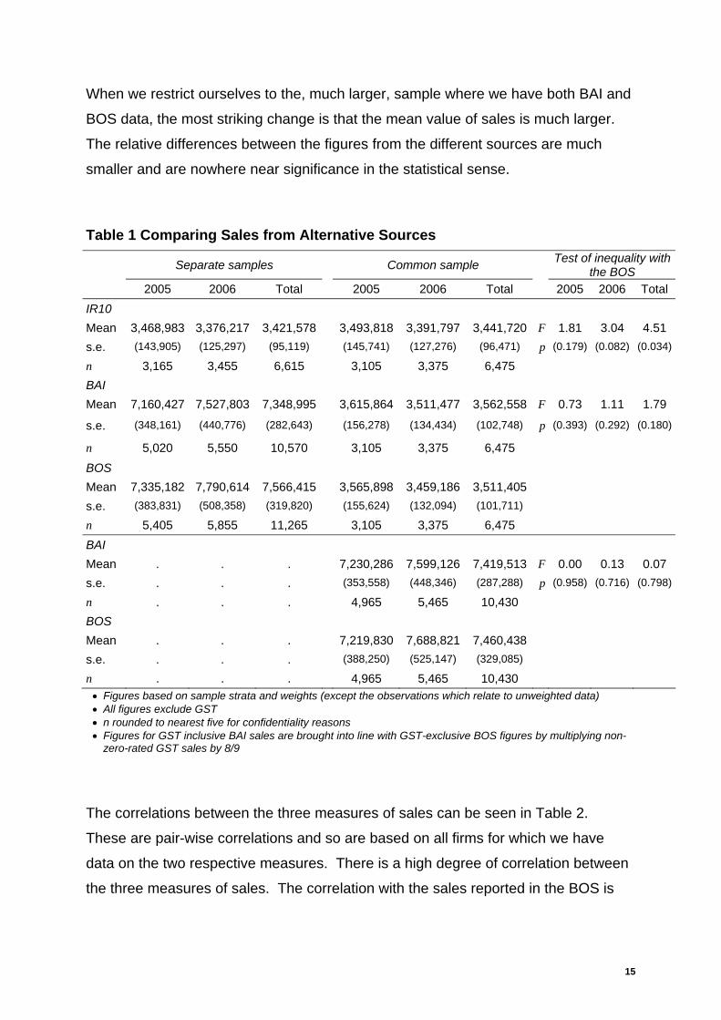
When we restrict ourselves to the, much larger, sample where we have both BAI and

BOS data, the most striking change is that the mean value of sales is much larger.

The relative differences between the figures from the different sources are much

smaller and are nowhere near significance in the statistical sense.

Table 1 Comparing Sales from Alternative Sources

Separate samples Common sample Test of inequality with the BOS

2005 2006 Total 2005 2006 Total 2005 2006 Total IR10 Mean 3,468,983 3,376,217 3,421,578 3,493,818 3,391,797 3,441,720 F 1.81 3.04 4.51 s.e. (143,905) (125,297) (95,119) (145,741) (127,276) (96,471) p (0.179) (0.082) (0.034)

n 3,165 3,455 6,615 3,105 3,375 6,475 BAI Mean 7,160,427 7,527,803 7,348,995 3,615,864 3,511,477 3,562,558 F 0.73 1.11 1.79

s.e. (348,161) (440,776) (282,643) (156,278) (134,434) (102,748) p (0.393) (0.292) (0.180)

n 5,020 5,550 10,570 3,105 3,375 6,475 BOS Mean 7,335,182 7,790,614 7,566,415 3,565,898 3,459,186 3,511,405 s.e. (383,831) (508,358) (319,820) (155,624) (132,094) (101,711) n 5,405 5,855 11,265 3,105 3,375 6,475 BAI Mean . . . 7,230,286 7,599,126 7,419,513 F 0.00 0.13 0.07 s.e. . . . (353,558) (448,346) (287,288) p (0.958) (0.716) (0.798)

n . . . 4,965 5,465 10,430 BOS Mean . . . 7,219,830 7,688,821 7,460,438 s.e. . . . (388,250) (525,147) (329,085) n . . . 4,965 5,465 10,430

• Figures based on sample strata and weights (except the observations which relate to unweighted data) • All figures exclude GST • n rounded to nearest five for confidentiality reasons • Figures for GST inclusive BAI sales are brought into line with GST-exclusive BOS figures by multiplying non-

zero-rated GST sales by 8/9

The correlations between the three measures of sales can be seen in Table 2.

These are pair-wise correlations and so are based on all firms for which we have

data on the two respective measures. There is a high degree of correlation between

the three measures of sales. The correlation with the sales reported in the BOS is

15

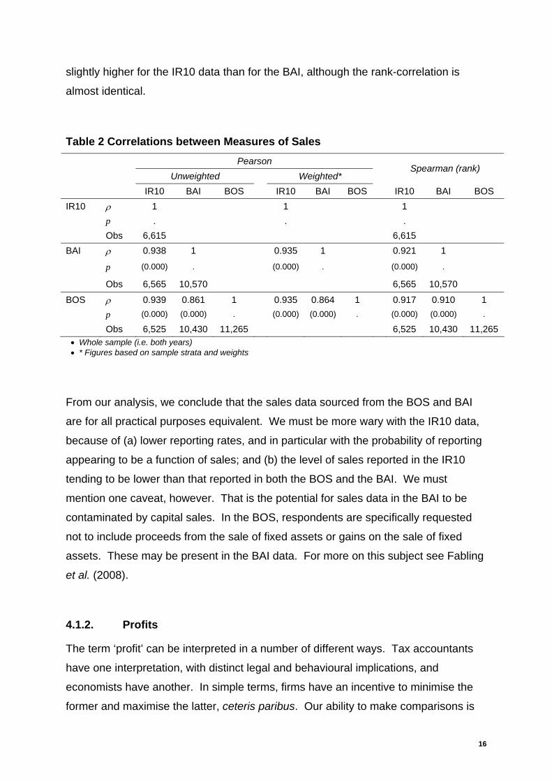
slightly higher for the IR10 data than for the BAI, although the rank-correlation is

almost identical.

Table 2 Correlations between Measures of Sales Pearson Unweighted Weighted*

Spearman (rank)

IR10 BAI BOS IR10 BAI BOS IR10 BAI BOS IR10 ρ 1 1 1 p . . . Obs 6,615 6,615 BAI ρ 0.938 1 0.935 1 0.921 1

p (0.000) . (0.000) . (0.000) .

Obs 6,565 10,570 6,565 10,570

BOS ρ 0.939 0.861 1 0.935 0.864 1 0.917 0.910 1 p (0.000) (0.000) . (0.000) (0.000) . (0.000) (0.000) .

Obs 6,525 10,430 11,265 6,525 10,430 11,265 • Whole sample (i.e. both years) • * Figures based on sample strata and weights

From our analysis, we conclude that the sales data sourced from the BOS and BAI

are for all practical purposes equivalent. We must be more wary with the IR10 data,

because of (a) lower reporting rates, and in particular with the probability of reporting

appearing to be a function of sales; and (b) the level of sales reported in the IR10

tending to be lower than that reported in both the BOS and the BAI. We must

mention one caveat, however. That is the potential for sales data in the BAI to be

contaminated by capital sales. In the BOS, respondents are specifically requested

not to include proceeds from the sale of fixed assets or gains on the sale of fixed

assets. These may be present in the BAI data. For more on this subject see Fabling

et al. (2008).

4.1.2. Profits

The term ‘profit’ can be interpreted in a number of different ways. Tax accountants

have one interpretation, with distinct legal and behavioural implications, and

economists have another. In simple terms, firms have an incentive to minimise the

former and maximise the latter, ceteris paribus. Our ability to make comparisons is

16

subject to data availability. GST-based data does not contain information to allow a

comparison with the BOS. For a comparison of administrative and survey measures

of profits, we use data from IR10 returns. One disadvantage of this is that it reduces

our sample size (because of the lower response/submission rates for iR10 returns).

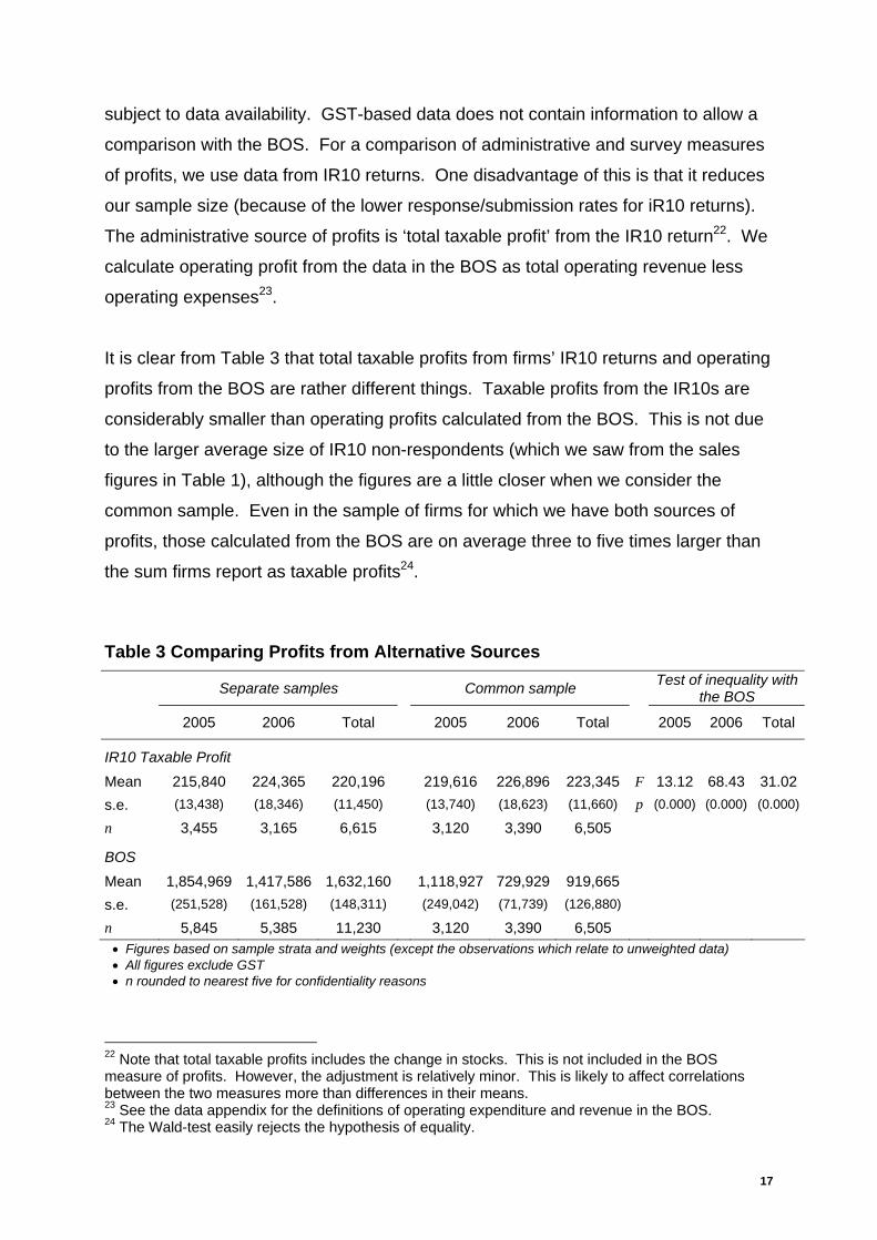
The administrative source of profits is ‘total taxable profit’ from the IR10 return22. We

calculate operating profit from the data in the BOS as total operating revenue less

operating expenses23.

It is clear from Table 3 that total taxable profits from firms’ IR10 returns and operating

profits from the BOS are rather different things. Taxable profits from the IR10s are

considerably smaller than operating profits calculated from the BOS. This is not due

to the larger average size of IR10 non-respondents (which we saw from the sales

figures in Table 1), although the figures are a little closer when we consider the

common sample. Even in the sample of firms for which we have both sources of

profits, those calculated from the BOS are on average three to five times larger than

the sum firms report as taxable profits24.

Table 3 Comparing Profits from Alternative Sources

Separate samples Common sample Test of inequality with the BOS

2005 2006 Total 2005 2006 Total

2005 2006 Total

IR10 Taxable Profit Mean 215,840 224,365 220,196 219,616 226,896 223,345 F 13.12 68.43 31.02s.e. (13,438) (18,346) (11,450) (13,740) (18,623) (11,660) p (0.000) (0.000) (0.000)

n 3,455 3,165 6,615 3,120 3,390 6,505

BOS Mean 1,854,969 1,417,586 1,632,160 1,118,927 729,929 919,665 s.e. (251,528) (161,528) (148,311) (249,042) (71,739) (126,880) n 5,845 5,385 11,230 3,120 3,390 6,505

• Figures based on sample strata and weights (except the observations which relate to unweighted data) • All figures exclude GST • n rounded to nearest five for confidentiality reasons

22 Note that total taxable profits includes the change in stocks. This is not included in the BOS measure of profits. However, the adjustment is relatively minor. This is likely to affect correlations between the two measures more than differences in their means. 23 See the data appendix for the definitions of operating expenditure and revenue in the BOS. 24 The Wald-test easily rejects the hypothesis of equality.

17

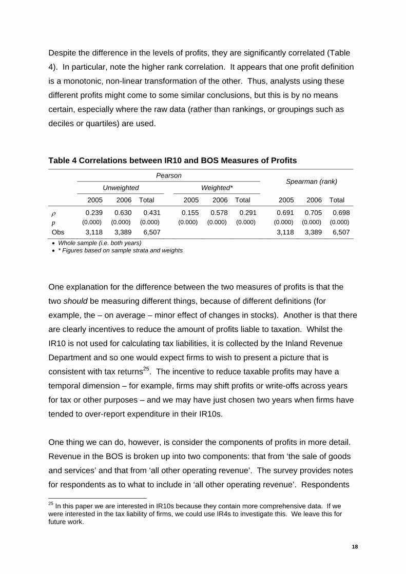
Despite the difference in the levels of profits, they are significantly correlated (Table

4). In particular, note the higher rank correlation. It appears that one profit definition

is a monotonic, non-linear transformation of the other. Thus, analysts using these

different profits might come to some similar conclusions, but this is by no means

certain, especially where the raw data (rather than rankings, or groupings such as

deciles or quartiles) are used.

Table 4 Correlations between IR10 and BOS Measures of Profits

Pearson

Unweighted Weighted* Spearman (rank)

2005 2006 Total 2005 2006 Total 2005 2006 Total

ρ 0.239 0.630 0.431 0.155 0.578 0.291 0.691 0.705 0.698p (0.000) (0.000) (0.000) (0.000) (0.000) (0.000) (0.000) (0.000) (0.000)

Obs 3,118 3,389 6,507 3,118 3,389 6,507• Whole sample (i.e. both years) • * Figures based on sample strata and weights

One explanation for the difference between the two measures of profits is that the

two should be measuring different things, because of different definitions (for

example, the – on average – minor effect of changes in stocks). Another is that there

are clearly incentives to reduce the amount of profits liable to taxation. Whilst the

IR10 is not used for calculating tax liabilities, it is collected by the Inland Revenue

Department and so one would expect firms to wish to present a picture that is

consistent with tax returns25. The incentive to reduce taxable profits may have a

temporal dimension – for example, firms may shift profits or write-offs across years

for tax or other purposes – and we may have just chosen two years when firms have

tended to over-report expenditure in their IR10s.

One thing we can do, however, is consider the components of profits in more detail.

Revenue in the BOS is broken up into two components: that from ‘the sale of goods

and services’ and that from ‘all other operating revenue’. The survey provides notes

for respondents as to what to include in ‘all other operating revenue’. Respondents 25 In this paper we are interested in IR10s because they contain more comprehensive data. If we were interested in the tax liability of firms, we could use IR4s to investigate this. We leave this for future work.

18

are asked to include: ‘renting and leasing income’, ‘government grants received for

operating purposes’, and ‘interest and dividend revenue’. They are asked to exclude:

‘proceeds from the sale of fixed assets’ and ‘gains on the sale of fixed assets’. In the

IR10 form, income includes ‘gross income from sales and/or services’, ‘interest

received’, ‘dividends’, ‘rental and lease payments’, and ‘other income’26. The

instructions in the BOS closely match the boxes in the IR10. The only exception is

that the BOS mentions ‘government grants received for operating purposes’. No

explicit mention of government grants is made in the notes on the final page of the

IR10 form. The notes for ‘other income’ ask filers to: ‘Include all other sources of

income that would be shown in the trading or the profit and loss account. This

includes, for example, subvention receipts, depreciation recovered, deferred income

assessed this year, income spread forward into this year and Rural Bank suspensory

loans forgiven’. There is also no mention of grants in the Guidelines for completing

the IR 10 document (IR10G) that IRD produces.

The top section of Table 5 shows income/revenue in the BOS and IR10, broken

down into sales and other income/revenue (for the IR10, this is the sum of the four

non-sales items). We can see that each of the three items is recorded as being

higher in the BOS than in the IR10. However, our F-tests suggest that we can accept

the hypothesis that firms report higher sales in the BOS (at the 5% level), but not

other income. In part, this latter result is due to the much higher variance in reported

‘other operating expenditure’ in the BOS. This could be taken as prima facie

evidence for greater uncertainty among BOS respondents as to what they should

include in their answer to this question. Nevertheless, other income/revenue is on

average twice as high in the BOS as it is in the IR10. This accounts for a large

proportion of the additional total income/revenue reported in the BOS. The test for

the difference in means for total revenue is just significant at the 10% level.

26 Note that the second page of the IR10 (‘balance sheet items’) includes boxes for losses and gains on disposal of fixed assets.

19

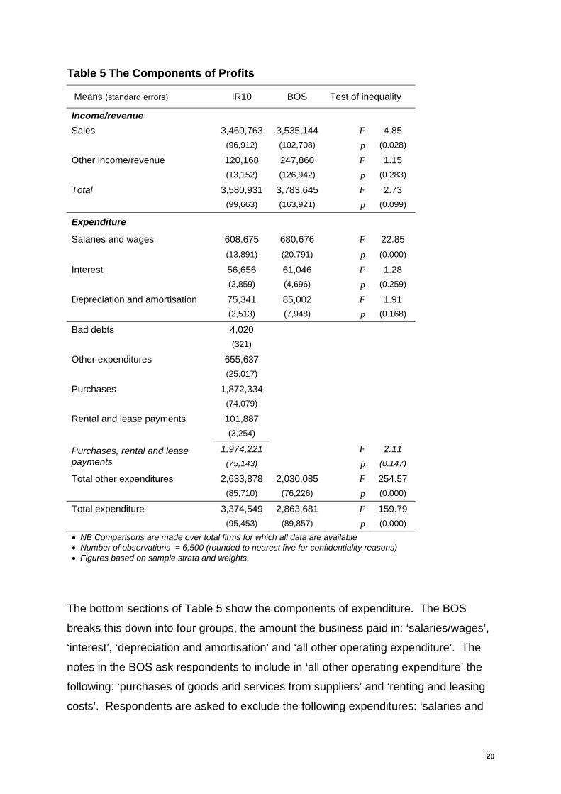
Table 5 The Components of Profits

Means (standard errors) IR10 BOS Test of inequality

Income/revenue Sales 3,460,763 3,535,144 F 4.85 (96,912) (102,708) p (0.028)

Other income/revenue 120,168 247,860 F 1.15 (13,152) (126,942) p (0.283)

Total 3,580,931 3,783,645 F 2.73 (99,663) (163,921) p (0.099)

Expenditure

Salaries and wages 608,675 680,676 F 22.85 (13,891) (20,791) p (0.000)

Interest 56,656 61,046 F 1.28 (2,859) (4,696) p (0.259)

Depreciation and amortisation 75,341 85,002 F 1.91 (2,513) (7,948) p (0.168)

Bad debts 4,020 (321) Other expenditures 655,637 (25,017) Purchases 1,872,334 (74,079) Rental and lease payments 101,887 (3,254)

1,974,221 F 2.11 Purchases, rental and lease payments (75,143) p (0.147)

Total other expenditures 2,633,878 2,030,085 F 254.57 (85,710) (76,226) p (0.000)

Total expenditure 3,374,549 2,863,681 F 159.79 (95,453) (89,857) p (0.000) • NB Comparisons are made over total firms for which all data are available • Number of observations = 6,500 (rounded to nearest five for confidentiality reasons) • Figures based on sample strata and weights

The bottom sections of Table 5 show the components of expenditure. The BOS

breaks this down into four groups, the amount the business paid in: ‘salaries/wages’,

‘interest’, ‘depreciation and amortisation’ and ‘all other operating expenditure’. The

notes in the BOS ask respondents to include in ‘all other operating expenditure’ the

following: ‘purchases of goods and services from suppliers’ and ‘renting and leasing

costs’. Respondents are asked to exclude the following expenditures: ‘salaries and

20

wages’, ‘purchase of fixed assets’, ‘interest and finance costs’, ‘depreciation or

amortisation’, and ‘losses on sales of fixed assets’. The IR10 form has sixteen

expense categories (these are detailed in the appendix, with descriptive statistics in

Table 21). It has categories that appear to exactly mirror the three specific

categories in the BOS. One slight difference is that respondents to the BOS are

asked to include employee ACC contributions in the total amount the business paid

for salaries and wages. In the IR10, respondents are asked to include ACC levies in

‘other expenses’.

For the specific categories in the BOS where we can make a direct comparison, firms

report slightly higher amounts for expenses than in the IR10. However, the only

category for which this is statistically significant is for salaries and wages. This is in

part due to the additional ACC costs included in the BOS salaries and wages.

However, this is not sufficient to explain the majority of the difference27.

Despite the similarities between the specific categories of expenses – and indeed the

tendency for firms to report slightly higher values in the BOS than in their IR10 –

overall expenses are much higher in the IR10 returns than in the BOS. As we can

see from the table, the majority of the remainder of expenses is made up of

purchases. Note that if we sum the IR10 categories corresponding to the two

examples of ‘other operational expenditure’ provided in the BOS notes – ‘purchases’

and ‘rental and leasing costs’ – the figures are much more similar than the overall

total of other expenditures. Indeed, we cannot reject the hypothesis that they are the

same in our Wald test.

This raises the question of how respondents deal with ‘other’-type categories in such

forms. One hypothesis is that they have an actual figure for the total amount. They

then remove the components they are asked to supply and put the figure for the

remainder in the ‘other’ box. We call this the ‘top down’ response. Another is that

respondents consider the total as the sum of the parts. We call this the ‘bottom up’

response. In cases where the totals are clearly defined in the eyes of the

27 ACC contributions vary across industries, but the average employer levy was around 1.2% of payroll in 2005/6 and 2006/7, and the average earners levy was 1.1% in 2005/6 and 1.2% in 2006/7. Source: Letter entitled ‘2007/08 ACC levies’ from Hon Ruth Dyson, Minister for ACC, 15 December 2006.

21

respondents, one would expect respondents to calculate the ‘other’ category using

the top down approach. If there is some ambiguity – in either the total or the other

component categories – respondents may employ the bottom up method, or a

combination of the two. In the top down case, the instructions for what to include in

the other category are surplus if what should be included in total and the other

component categories is clear. In the bottom up case, respondents rely much more

on the instructions in the questionnaire. It is possible that respondents see the

examples of ‘other operational expenditure’ as an enumeration of the contents (i.e. a

complete listing of all the items that should be included in the category). The results

of our analysis presented in Table 5 show that we can reject the hypotheses that

either the ‘total’ or the ‘other’ expense categories in the BOS and IR10 are the same

across firms. However, to reiterate the previous paragraph, we cannot reject the

hypothesis that respondents report the same value in the ‘other expenditure’

category in the BOS as they do in the IR10 categories that are specifically itemised

as examples of BOS 'other expenditure'. This is prima facie evidence for the ‘bottom

up’ approach, or what we might call an ‘enumeration effect’28.

One potential culprit that we noted above for differences between the profits is the

writing-off of bad debts. Firm might choose to write-off bad debts in good years in

order to offset them as expenses against profits. These will show up in the financial

accounts in the balance sheets as current assets until they are written-off, when they

appear on the profit and loss account as expenses. Because of the tax incentive to

write bad debts off in good years, one might expect the writing-off of bad debts to be

pro-cyclical. This may be the case, but the size of bad debts expenses is rather

small compared to the difference between total expenditures as recorded in firms’

BOS and IR1029. According to the IR10, over half (55%) of operating expenses is

made up of purchases. The next largest proportion (18%) is made up of salaries and

wages. Of the remainder, around half is made up of fourteen expense categories

28 There is support for the idea on an enumeration effect from other analyses of SNZ-run surveys. Specifically, Fabling (2007b) investigates differences in reported R&D expenditure between BOS and R&D surveys by matching unedited responses across the two surveys. He finds that R&D survey responses tend to be higher than BOS responses and that, in part, ‘[t]he R&D survey elicits higher aggregates because component expenditure is enumerated over several pages of expense categories. Thus a survey purely on R&D may “focus the mind” and aid recall of, or encourage fuller disclosure of, activities which are then counted as R&D.’ 29 It might be the case that potential debts were written off in earlier years, but we leave this for later work.

22

named in the IR10, none of which contribute more than 3%30. The other half is the

ubiquitous ‘other expenses’ category.

Our analysis suggests that the majority of the difference between total taxable profits,

as recorded in the IR10, and operating profits in the BOS is due to the much higher

amounts recorded as expenses in the IR10. The obvious explanation for this is that

there are incentives for firms to reduce their tax liability by ensuring expenses are as

high as reasonably possible and income as low. Note that the IR10 is ‘designed to

collect information for statistical purposes’ (SNZ: IR10G: IR10 Guide) and not for

calculating tax. Another potential explanation for the difference is that there are

many more expense categories listed in the IR10 than in the BOS and this may

stimulate respondents to include more expenses in the IR10 (what we have called

the ‘enumeration effect’. In the language of Tourangeau et al. (2000), this may cause

problems with comprehension, causing respondents to either retrieve the wrong

information or judge that some of the information retrieved does correspond to the

data required. When we have compared the sum of the two expenses listed in the

BOS notes as components of ‘other operating expenditure’ – purchases and rental/

lease payments – with equivalent entries in the IR10, the results are quite similar.

4.1.3. Employment

Employment raises rather different issues to the financial variables. Employees can

be full or part-time; they can be temporary or permanent; they can be employed for

the whole of the year or part of it; some staff may not be employees (e.g. working

proprietors). In this paper our administrative measure of employment is made up of

two components: employees and working proprietors. Our measure of employees is

defined as an average of twelve-monthly PAYE employee counts in the year (known

as rolling mean employment, or RME31). This takes into account some of these

complications (e.g. part-year working), but not others (e.g. variations in hours worked,

such as the difference between full-time and part-time workers). Our measure of

working proprietors also comes from the LEED, but is rather more complex. It is a

30 For a full breakdown of the revenues and expenses collected on page 1 of the IR10 return, see

in the appendix. Table 2131 Note that it is not a true rolling mean over the year, since the monthly figures are taken as of 15th of the month, rather than an average over the month.

23

count of the number of self-employed persons who are paid taxable income during

the tax year. This is based on a number of IRD forms and is calculated on a March

year-end basis. For more information on the calculation of this figure, see the data

appendix.

Employment in the BOS is broken down into full-time (working 30 hours or more per

week) and part-time working proprietors and employees. Respondents are asked to

exclude contractors from employees. In the 2006 survey respondents are also asked

to include the total headcount (FT and PT) of workers32. We calculate two measures

of employment from the BOS. Our headcount measure is simply the sum of FT and

PT workers. Our FTE measure assumes that PT workers work half the hours of FT

workers (i.e. FTE=FT+0.5PT).

The comparison of employment from the LEED and BOS employment is presented in

Table 6. Looking first at working proprietors, the BOS headcount measure is higher

than the equivalent LEED count, with the BOS FTE measure somewhere in between.

This result is fairly independent of whether we consider the separate sample or focus

on the set of firms for whom we have both figures. In general, firms tend to include

around half an extra working proprietor in their responses to the BOS that one would

expect given the LEED data. This result is statistically significant at the 0.1% level.

This may in part be due to the fact that some of the working proprietors included in

the BOS do not draw an income from the firm during the year. However, on the

contrary, it is also possible for individuals to be included in the LEED measure of

working proprietors because they receive non-wage income. One might expect

some of these to be excluded the BOS working proprietor count. Another

explanation is that some respondents to the BOS included some contractors (they

may not have realised a staff member was a contractor, or may have misread the

instructions).

32 For more on this see the discussion below and the data appendix.

24

Table 6 Comparison of PAYE-based RME and Self-reported Employment in BOS

Separate samples Common sample Test of inequality 2005 2006 Total 2005 2006 Total 2005 2006 Total LEED Working Proprietors Mean 1.419 1.389 1.404 1.419 1.389 1.404

s.e. 0.040 0.040 0.028 0.040 0.040 0.028 n 5,095 5,640 10,735 5,095 5,640 10,735 BOS Working Proprietors (Headcount) Mean 2.106 1.850 1.976 2.132 1.857 1.991 F 60.8 63.1 118.72

s.e. 0.083 0.055 0.050 0.087 0.056 0.051 p (0.000) (0.000) (0.000)

n 5,470 5,950 11,420 5,095 5,640 10,735

BOS Working Proprietors (FTE) Mean 1.878 1.689 1.782 1.919 1.700 1.807 F 31.8 31.2 60.53

s.e. 0.079 0.051 0.047 0.084 0.051 0.049 p (0.000) (0.000) (0.000)

n 5,470 5,950 11,420 5,095 5,640 10,735

LEED Employees Mean 28.04 27.91 27.97 28.04 27.91 27.975

s.e. 1.203 1.136 0.826 1.203 1.136 0.826 n 5,095 5,640 10,735 5095 5640 10735 BOS Employees (Headcount) Mean 34.31 30.68 32.47 35.14 30.63 32.824 F 2.61 33.4 5.09

s.e. 4.288 1.338 2.220 4.593 1.373 2.343 p (0.106) (0.000) (0.024)n 5,470 5,950 11,420 5,095 5,640 10,735 BOS Employees (FTE) Mean 29.49 26.31 27.88 30.32 26.3 28.258 F 0.27 20.9 0.02

s.e. 4.197 1.111 2.144 4.496 1.142 2.265 p (0.602) (0.000) (0.895)n 5,470 5,950 11,420 5,095 5,640 10,735

LEED Total Employment Mean 29.46 29.3 29.38 29.46 29.29 29.371

s.e. 1.199 1.132 0.823 1.199 1.132 0.823 n 5,095 5,640 10,735 5,095 5,640 10,735 BOS Total Employment (Headcount) Mean 36.41 32.52 34.44 37.27 32.47 34.805 F 3.16 45.8 6.38

s.e. 4.291 1.339 2.221 4.596 1.374 2.345 p (0.076) (0.000) (0.012)

n 5,470 5,950 11,420 5,095 5,640 10,735 BOS Total Employment (FTE) Mean 31.37 27.98 29.65 32.24 27.99 30.06 F 0.4 13.7 0.1

s.e. 4.199 1.112 2.145 4.499 1.143 2.267 p (0.525) (0.000) (0.748)

n 5,470 5,950 11,420 5,095 5,640 10,735 • NB ‘Test of inequality’ is with LEED figure • Figures based on sample strata and weights (except the observations which relate to unweighted data)

25

Turning to the employee numbers, we can see that there is something slightly

unusual going on in the BOS sample for 2005. The variance (and thus the standard

error of the mean33) is considerably higher for BOS employee numbers in 2005 than

for either the same question(s) in the BOS 2006 or the LEED RME counts in both

years. It should be noted that the question in the BOS changed slightly between

2005 and 2006. The changes were mainly formatting, with boxes and notes moved

slightly. One major change was that in 2006, respondents were asked to include a

total in addition to the numbers of part-time and full-time working proprietors and

employees. These changes were made in response to problems survey respondents

appeared to have with the employment questions34. Because of the higher variance

in responses to the 2005 survey, we cannot quite distinguish statistically between the

BOS headcount and the LEED RME figures (at standard statistical levels), despite

the fact that the respondents to the BOS appear to record 25% more employees than

one would expect given the LEED figure. For 2006, the standard error of the mean

of BOS employment drops to something much more akin to that for the LEED figure.

Furthermore, the mean estimate of employment also drops to something closer to the

LEED figure. Nevertheless, respondents to the BOS still report employment around

10% higher than the figure obtained from PAYE records; a difference that is highly

statistically significant. The BOS FTE measure of employment is much closer to the

LEED figure in both years, although this difference is still statistically significant in

2006.

As one would expect, given the relative numbers of working proprietors and

employees, the results for total employment are similar for those for employees. One

difference is that now the difference between the BOS headcount and LEED RME

figure for total employment is statistically significant at the 10% level (although not

the 5% level).

Why are the BOS headcount figures higher, but the FTE figures close to the LEED

RME figures? Is there a tendency to over-report temporary workers in the BOS, or is 33 Note that this equal to the standard deviation divided by the square root of the number of observations. 34 Note, however, that the main issue with the employment questions in the BOS was with the following question, an occupational breakdown of employment. Nevertheless, it is possible that respondents gone back to the question requesting total employment numbers after providing the occupational breakdown.

26

there some other explanation? There are a number of potential explanations,

relating to the individuals who are included, the time frame over which individuals are

counted and the type of employment. LEED has a very specific population: those for

whom a PAYE form is submitted. Individuals will not be included in the PAYE

records if they work without pay. Also students earning less than $20 per week, or

no more than $1,400 per year may not be included (although this depends on the

practices of their employer).

The BOS figure is a spot estimate of employment. Respondents (either from the

Human Resources department or if they do not have one, the General Manager) are

asked: ‘As at the end of the last financial year, how many staff worked for this

business?’ LEED RME is on the other hand an average of monthly spot estimates

over the whole year. There are at least two reasons why this might lead to a higher

value being reported in the BOS than in the LEED. The first is that BOS respondents

answer exactly the question they are asked, and provide a true estimate of staff

numbers at that particular point of time, but employment tends to peak at the end of

the financial year. There is some reason to expect this to be the case as most

financial years end in March and so this might include seasonal employment at the

end of summer. The second is that BOS respondents suffer a recollection bias and

do in fact report their recollection of staff (either individually or the numbers involved)

over the year and misattribute the times over which they are employed. This is

qualitatively similar to the concept of ‘telescoping’ in the survey literature. An

example of this is when respondents misreport times for which they were employed

or unemployed (Akerlof and Yellen, 1985; Mathiowetz, 1986). The result of this

consideration of total staff over a longer period (e.g. the whole year) is to

overestimate the proportion of staff that were employed at the end of the financial

year35.

The correlations between the different measures of employment are all highly

statistically significant (Table 736). The correlations between BOS and LEED

35 It would be possible for future work to consider this in more detail by comparing salaries and wages as recorded in BOS (and indeed IR10s) with that from LEED and looking at the monthly LEED data. 36 Note that the correlation coefficient for both years’ data combined and the unweighted Pearson correlation are included in the Appendix to this paper.

27

employment are little different when we consider the BOS FTE and headcounts

measures, although the difference is slightly larger in 2005 than in 2006.

There is a relatively low degree of correlation between the survey and administrative

measures of working proprietors, particularly in 2005, although the much higher rank

correlation suggests that the relationship between the two is a non-linear but fairly

monotonic transformation (i.e. it affects different parts of the distribution differently,

but has much less of an impact on their ordering within the distribution).

There is a much higher correlation between the BOS measures of employees and

total employment in both years. Once more it is much lower in 2005 than in 2006,

although the rank correlations are almost identical.

Overall these results suggest that the two sources of data are very similar in 2006,

with a tendency for the BOS figures to be slightly larger than those from LEED.

There is clearly quite a difference between the 2005 and 2006 responses. Our

reading of the results, in combination with discussions with SNZ staff, suggests that

there were problems with the responses to the employment questions in 2005.

28

Table 7 Correlations between Measures of Employment

Pearson Spearman (rank)

2005 2006 2005 2006 Observations

ρ p ρ p ρ p ρ p 2005 2006

BOS Headcount with LEED Working proprietors 0.073 (0.000) 0.166 (0.000) 0.537 (0.000) 0.525 (0.000) 5,095 5,640

Employees 0.351 (0.000) 0.938 (0.000) 0.910 (0.000) 0.911 (0.000) 5,095 5,640 Total Employment 0.351 (0.000) 0.938 (0.000) 0.917 (0.000) 0.924 (0.000) 5,095 5,640

BOS FTE with LEED Working proprietors 0.070 (0.000) 0.183 (0.000) 0.531 (0.000) 0.525 (0.000) 5,095 5,640

Employees 0.284 (0.000) 0.946 (0.000) 0.904 (0.000) 0.913 (0.000) 5,095 5,640 Total Employment 0.284 (0.000) 0.946 (0.000) 0.910 (0.000) 0.927 (0.000) 5,095 5,640

BOS Headcount with BOS FTE Working proprietors 0.995 (0.000) 0.983 (0.000) 0.980 (0.000) 0.988 (0.000) 5,470 5,950

Employees 0.995 (0.000) 0.986 (0.000) 0.985 (0.000) 0.990 (0.000) 5,470 5,950 Total Employment 0.995 (0.000) 0.986 (0.000) 0.983 (0.000) 0.989 (0.000) 5,470 5,950

4.1.4. Productivity

Productivity is an important determinant of the wealth and welfare of economies

(Prescott, 1998; Kneller and Stevens, 2002). Because of this, it is a key variable of

interest to economists and policy-makers alike. When we consider the impact of

factors such as competition, innovation or management capability on the economy,

one of the key indicators is productivity. Having good measures of productivity

therefore is extremely important.

In this paper we shall focus on the log of labour productivity37, equal to the log of

value-added minus the log of employment. We construct a measure of labour

productivity from both administrative data38 and from the BOS39. Our measure of

37 We use log productivity for comparability with other work (e.g. Fabling et al., 2008) and because of the skewed distribution of productivity 38 Using sales of goods and services minus purchases from the BAI as value added (adjusted for changes in stock from IR10s where possible), and RME from LEED. See data appendix for more details. 39 Using sales of goods and services minus total other operating expenditure from BOS as value-added and BOS total employment.

29

productivity is essentially made up of three variables - sales, purchases and

employment – each of which may be measured with error. The impact of these

individual errors on the measurement of productivity – and hence our comparison of

the two measures – is ambiguous, as it depends on the correlation between the

errors, as well as their size. Nevertheless, our expectation is that overall

measurement error will be below that of the sum of the individual components, and

hence the BOS and administrative data will be more similar.

As we can see from Table 8, the two measures are significantly correlated with each

other, but the value of productivity obtained from the BOS is statistically significantly

higher than that obtained from the BAI. One reason for the difference might be the

contamination of sales and purchases data in the BAI by capital sales and

expenditure (c.f. Fabling et al, 2008). However, it is not certain this will bias the sales

data in either direction. Indeed, on average one would expect sales and purchases

of capital goods to approximately even out40. In the BOS, respondents are

specifically requested not to include the purchase of fixed assets or losses on sales

of fixed assets. Because of this, one would expect value-added – and hence

productivity – to be higher in the BOS measure, ceteris paribus. However, our

measure of purchases in the BOS is ‘all other operating expenditure’ and so may

include other expenses (although our discussion of Table 5 suggests that many of

the other expenses are not included). Turning to the employment side of the

productivity calculation, recall from our discussion of Table 6 that our headcount

measure of employment is significantly higher in the BOS than in the LEED, which

would tend to reduce the measure of labour productivity calculated from the BOS

financials relative to that from the BAI/LEED.

40 It would be possible to use gains and losses on the sale of assets from the back page of the IR10 to gain a further insight into this issue.

30

Table 8 Comparison of Productivity from Administrative Data and the BOS

Correlations

Mean Std. Err.

Test of inequality Pearson Spearman

2005 n 9,715 BAI/LEED 10.65 (0.018) F 206.38 ρ 0.5128 0.6037 BOS 10.93 (0.021) p (0.000) p (0.000) (0.000)

2006 n 4,615 BAI/LEED 10.64 (0.026) F 114.89 ρ 0.5014 0.5990 BOS 10.93 (0.029) p (0.000) p (0.000) (0.000)

2005 & 2006 n 5,100

BAI/LEED 10.66 (0.026) F 93.74 ρ 0.5238 0.6079 BOS 10.93 (0.029) p (0.000) p (0.000) (0.000)

• Weighted and stratified (except Spearman correlations)

Whilst we might be worried that labour productivity calculated using the BOS is

significantly different from that calculated from the BAI data, we should caution that

we are seldom interested in the level of productivity per se, except to make

comparisons between firms. We are interested mainly in relative productivity, i.e. in

understanding why some firms are more productive than others. The fact that they

are significantly correlated – despite the definitional differences – and in particular the

high rank correlation suggests that any policy prescriptions based upon either

measures will not give results that are too far different from those based on the other.

However, it would be useful to understand the differences in more detail.

4.2. Comparing Self-reported Subjective/Qualitative and Quantitative Data

In this section we turn our attention to subjective measures of firm performance.

Such measures are often the only information analysts have at their disposal and so

their correlation with more objective – but harder to come by – measures of firm

performance is of considerable interest. In a manner similar to Forth and McNabb

(2008a) we compare self-reported qualitative, subjective measures of performance

with ‘objective’ measures derived from financial information reported in the BOS.

31

Table 9 Self-reported relative Profitability and Productivity Profitability Productivity Unweighted Weighted Unweighted Weighted

2005 Lower than competitors 10.7 9.7 5.0 4.1 On a par with competitors 42.9 45.3 46.2 46.5 Higher than competitors 22.6 17.6 27.0 24.4 Don’t Know 23.8 27.4 21.8 25.0

2006

Lower than competitors 11.3 12.0 4.8 4.6

On a par with competitors 45.5 47.2 47.9 48.0 Higher than competitors 21.5 16.1 27.5 23.5 Don’t Know 21.7 24.7 19.9 23.9

2005 & 2006 Lower than competitors 11.0 10.9 4.9 4.4 On a par with competitors 44.3 46.3 47.1 47.3 Higher than competitors 22.0 16.8 27.3 23.9 Don’t Know 22.7 26.0 20.8 24.5 • Table refers to the BOS Question 38: ‘How do you think this business compares to its major competitors on

each of the following? Profitability; Productivity’

The two subjective measures of performance we consider are relative profitability

and productivity. Question 38 of the BOS asks firms how they think their business

compares with its major competitors against both these metrics. Taken at face value,

Table 9 confirms our suspicion that respondents tend on average to consider

themselves above average. Almost half of the respondents in both years and for

both questions think of themselves as ‘on a par with competitors’. Around twice as

many firms reported themselves as more profitable than their competitors than less41,

and around six times as many feel they are more productive than less. This is

consistent with the results for output per head and value-added per head in the

Workplace Employment Relations Survey (WERS) reported in Forth and McNabb

(2008a), although the respondents to the WERS have five choices (‘A lot below

average’, ‘Below average’; ‘About average’; ‘Above average’; and ‘A lot above

average’). The majority of (weighted) responses (over 80%) in Forth and McNabb

41 Although once we weight the data, we find this difference shrinks, particularly in 2006.

32

are either ‘About average’ or ‘above average’ (with the split being roughly equal

between the two)42.

One explanation for this apparent upward bias is the large number of firms that

answer ‘don’t know’ to this question (Fabling and Grimes, 2007, find striking

similarities between the ‘don’t know’ group and a combined ‘low/average’ group). For

example, firms that reported that they did not know might be less profitable or

productive, and either (a) the factors that prevent them knowing are correlated with

their low competitiveness (i.e. managers who cannot see how well the firm is doing

are not good managers, which makes the firm perform less well)43 or (b) they know

the truth and cannot bring themselves to admit it in writing. We can get a better

understanding of whether the second explanation is true, by comparing the

subjective measures of profitability and productivity with objective ones. This we now

do.

4.2.1. Productivity

Considering productivity first, we can compare the subjective estimate of (relative)

productivity with a labour productivity measure from the financial information from

Part i. of the BOS. There are a number of ways in which respondents could be

answering subjective questions with respect to productivity. First, there are issues

about the appropriate denominator, i.e. whether firms are considering labour or some

type of multi-factor productivity. Second, there is the issue of the appropriate

numerator, e.g. sales or value-added. Not all respondents will have economics

degrees and so this question is open to multiple interpretations. Earlier evidence

(Forth and McNabb, 2008a) suggests that managers’ reporting of subjective

measures of profitability are closer to objective measures than they are of

productivity. Forth and McNabb suggest that this reflects greater clarity as to what is

being asked about profitability than productivity. However, as we have noted in

footnote 42 above, Forth and McNabb do not report the proportion of WERS

42 Note, however, that Forth and McNabb (2008a) do not quote the figures for the ‘no comparison possible’, ‘relevant data not available’ and ‘not answered’ groups. Forth and McNabb (2008b) do, however, for a larger group of firms (1,757 compared to around 500 in Forth and McNabb, 2008a, depending on which table one considers). These latter groups contribute around 11.5% of the total (larger) sample. For more on Forth and McNabb’s (2008a,b) results, see the discussion below. 43 See an earlier version of this paper (Fabling, Grimes and Stevens, 2007) for more on this subject.

33

respondents that are in the ‘no comparison possible’, ‘relevant data not available’ and

‘not answered’ groups. Forth and McNabb (2008b) do for productivity and 4.6% of

respondents state that no comparison is possible, 2.5% say that the relevant data are

not available and 4.5% did not answer (weighted figures). In the case of the BOS

more firms respond that they do not know their profitability than report they do not

know their relative productivity. It is interesting to note that more respondents report

that they do not know their relative productivity in the BOS than do in the WERS.

This may be because the WERS does not contain financial questions requiring the

respondent to either have access to the firm’s accounts or some knowledge of them,

as the BOS does. It may, therefore, be clearer to WERS respondents that such a

question is an estimate than it is for BOS respondents that have just filled in several

pages of information on income, expenditure, assets, liabilities and employment.

The mean values of labour productivity for each group, their standard errors and 95%

confidence intervals are presented in Table 10. Those who report their productivity is

lower than their competitors clearly have the lowest labour productivity, although the

difference is larger in 2005 than 2006. Those who believe they are more productive

than their competitors indeed appear to be more productive than those who believe

they are on a par with their competitors. Firms who report that they do not know how

their labour productivity compares with their competitors tend to be around or just

below the ‘on a par with’ group.

We can make this comparison more rigorous by performing Wald tests of the equality

of these estimates. As we can see from Table 11, we can accept the hypothesis that

the means of productivity of the three groups are different. We cannot distinguish the

productivity of firms in the ‘don’t know ‘ category from the ‘lower than’ or ‘on a par

with competitors’ groups, but we can from the ‘higher than competitors’ group.

34

Table 10 Subjective and Objective Self-reported Measures of Productivity Labour productivity, ln(VA)-ln(RME)

Mean Linearised Std. Error [95% conf. interval]

2005 Lower than competitors 10.57 (0.092) 10.39 10.75 On a par with competitors 10.95 (0.043) 10.87 11.04 Higher than competitors 11.04 (0.058) 10.93 11.15 Don’t Know 10.82 (0.057) 10.71 10.93

2006

Lower than competitors 10.84 (0.107) 10.63 11.05

On a par with competitors 10.87 (0.045) 10.79 10.96 Higher than competitors 11.09 (0.063) 10.96 11.21 Don’t Know 10.87 (0.044) 10.78 10.95

2005 & 2006 Lower than competitors 10.72 (0.075) 10.57 10.86 On a par with competitors 10.91 (0.031) 10.85 10.97 Higher than competitors 11.06 (0.043) 10.98 11.15 Don’t Know 10.84 (0.036) 10.77 10.91 • Table shows values of the log of labour productivity by subjective relative probability • Weighted and stratified

Table 11 Wald Tests of Equality

On a par with competitors

Higher than competitors

Don’t know (4)

F 5.70 16.04 2.28 Lower than competitors (1) p (0.017) (0.000) (0.131)

F 8.23 2.06 On a par with competitors (2) p (0.004) (0.151)

F 15.57 Higher than competitors (3) p (0.000)

Joint Wald tests 1=2=3 1=2=3=4

F 8.98 7.64 p (0.000) (0.000)

• Top section of table reports two-way Wald F-Test of inequality of means of productivity between groups along with probability that the difference is not significantly different from zero

• Bottom section joint test that three categories of relative productivity are equal and that these are jointly equal to the ‘don’t know’ category, respectively

• Weighted and stratified

35

This result is confirmed when we perform an OLS regression of labour productivity on

dummy variables representing the subjective relative productivity groups and the

‘don’t know’ category (with ‘On a par with competitors’ as the baseline group) (Table

12). The significant, negative coefficient on ‘lower’ confirms that firms that report

their productivity is lower than competitors indeed tend to have lower productivity

than firms that think they are just as (or more) productive than their competitors.

Likewise, firms that believe that they are more productive than their competitors

indeed tend to be so. Our results therefore support the thesis that the subjective

data have some predictive power and correlate with objective measures.

Table 12 Regression of Labour Productivity on Subjective Measure Observations 10,980 F 7.64 Population 68,793 p 0 Design d.f. 10,980 R2 0.008 Coef. s.e. t P>t Constant 10.912 0.031 348.07 0.000 Lower -0.195 0.082 -2.39 0.017 Higher 0.152 0.053 2.87 0.004 Don’t know -0.069 0.048 -1.44 0.151

• Table reports results of a linear regression where the dependent variable is the log of labour productivity. Independent variables are dummy variables representing the subjective relative productivity groups and the ‘don’t know category’ (with ‘On a par with competitors’ as the baseline group).

• Observations rounded to the nearest five for confidentiality reasons • Weighted and rounded

One of the great strengths of the LBD is its breadth. Because we have data from the

majority of economically significant firms in New Zealand, we can consider a more

interesting alternative measure of relative productivity – the productivity of the firm

relative to all off its actual competitors. The key question is how we define

competitors. This is no simple matter.

There are a number of reasons why one would suspect that it is difficult to define the

market within which firms operate and hence identify its competitors. Firms may

operate in more than one product market. They may compete locally, nationally or

internationally. It may be the case that some ANZSIC codes do not necessarily

correspond to definitions of a ‘market’ and this may vary not only by product type, but

36

also by firm. Previous work suggests that there is considerable heterogeneity in how

firms respond to questions where they are asked to compare themselves to their

competitors (e.g. Mason, 2005). Part of this is due to the nature of the products or

services firms are offering, part is due to the fact that firms often only compare

themselves to firms with which they fell they can compete. Firms producing a much

higher or lower quality product are frequently considered to be in a different market,

despite the fact that the ANZSIC classification of their operation is the same.

Notwithstanding these caveats, however, it is possible to consider firms with similar

industrial classifications. We examine two alternatives – defining the group of firms

in competition with the firm as all those in the 3-digit or 4-digit ANZSIC industry in

which the firm is situated. We calculate these measures in two ways. In the

‘unweighted’ calculation, we compare the firm’s productivity relative to the simple

mean of all firms in the 3- or 4-digit industry. In the ‘weighted’ version, we compare it

to the mean of all firms in the relevant industry, weighted by sales.

Table 13 Subjective and Objective Self-reported Measures of Relative Productivity (LBD)

Unweighted Weighted 3-digit 4-digit 3-digit 4-digit

Constant 0.367*** 0.346*** 10.599*** 10.577***

(0.019) (0.019) (0.023) (0.023) -0.080 -0.095 -0.089 -0.105 Lower than

competitors (0.084) (0.084) (0.095) (0.094) 0.153*** 0.132*** 0.200*** 0.197***Higher than

competitors (0.039) (0.038) (0.045) (0.045) -0.025 -0.023 -0.057 -0.059 Don’t Know (0.042) (0.041) (0.045) (0.045)

Observations 10,010 10,010 10,010 10,010 R2 0.008 0.007 0.012 0.012 F 6.385 5.302 9.098 9.142 p 0.563 0.474 0.334 0.273

• Standard errors in parentheses • * significant at 10%; ** significant at 5%; *** significant at 1% • Note that all results are weighted and stratified, ‘Unweighted’ and ‘Weighted’ column headers relate to method

of calculating industry average productivity

The results of this exercise are presented in Table 13. The first thing to note is the

consistency of results across the specifications. The coefficient on the ‘lower than’

variable is of the expected sign (negative), but is statistically insignificant across all

37

specifications. The coefficient on the ‘higher than’ variable is also the expected sign

(positive) and is statistically significant. The coefficient on the ‘don’t know’ variable is

even less significant that that on the ‘lower than’ variable. These results are similar

whether we use the 3- or 4-digit industry measure. The coefficient on the ‘higher

than’ category is higher when we use the weighted calculation.

4.2.2. Profitability

The picture is similar when we consider profitability (Table 14 to Table 16), where

profitability is defined as profits divided by sales44. Profitability certainly rises over

the groups of firms in each of the self-reported profitability groups. The picture is

consistent across years. Those in the ‘lower than competitors’ group have a

profitability that is around zero and even have slightly negative profitability on

average in 2005. This difference between groups is statistically significant and at

standard levels of significance (Table 15). The ‘don’t know’ group appears to be

equivalent to (or slightly lower than) the ‘average’ firm. The mean value of

profitability is statistically indistinguishable from the ‘on a par group’, even at the 10%

level. It is distinguishable from the ‘higher than’ group at the 1% level, but only at a

lower (7%) level from the ‘lower than’ group. These results again hold when we take

a multiple regression approach (Table 16)45.

44 Note that we exclude some extreme values from the figures presented in to Table 16. In particular, there is one very large negative value (i.e. an extremely large loss relative to sales).

Table 14

45 Because of the large differences in profits noted above between measures obtained from the BOS and IR10, we cannot produce the analogue to for profitability. Table 13

38

Table 14 Subjective and Objective Self-reported Measures of Profitability Profitability

Mean Linearised Std. Error [95% conf. interval]

2005 Lower than competitors -0.021 (0.070) -0.157 0.116 On a par with competitors 0.192 (0.026) 0.142 0.243 Higher than competitors 0.225 (0.028) 0.170 0.280 Don’t Know 0.132 (0.045) 0.043 0.221

2006 Lower than competitors 0.025 (0.044) -0.062 0.112

On a par with competitors 0.147 (0.025) 0.098 0.197 Higher than competitors 0.223 (0.019) 0.185 0.261 Don’t Know 0.076 (0.061) -0.044 0.197

2005 & 2006 Lower than competitors 0.005 (0.039) -0.072 0.082 On a par with competitors 0.169 (0.018) 0.134 0.204 Higher than competitors 0.224 (0.017) 0.190 0.258 Don’t Know 0.105 (0.038) 0.030 0.179 • Table shows values of profitability by subjective relative profitability • Weighted and stratified

Table 15 Wald Tests of Equality

On a par with competitors

Higher than competitors

Don’t know (4)

F 14.37 26.04 3.33 Lower than competitors (1) p (0.000) (0.000) (0.068)

F 4.88 2.34 On a par with competitors (2) p (0.027) (0.126)

F 8.20 Higher than competitors (3) p (0.004)

Join Wald tests 1=2=3 1=2=3=4 F 13.37 10.12 p (0.000) (0.000)

• Top section of table reports two-way Wald F-Test of inequality of means of productivity between groups along with probability that the difference is not significantly different from zero.

• Bottom section reports joint test that three categories of relative productivity are equal and that these are jointly equal to the ‘don’t know’ category, respectively.

• Whole sample (i.e. both years)

39

Table 16 Regression of Profitability on Subjective Measure Observations 10,995 F 10.12 Population 68,793 p 0 Design d.f. 10,995 R2 0.0023 Coef. s.e. t P>t Constant 0.169 0.018 9.36 0.000 Lower -0.164 0.043 -3.79 0.000 Higher 0.055 0.025 2.21 0.027 Don’t know -0.064 0.042 -1.53 0.126

• Table reports results of a linear regression where the dependent variable is profitability. Independent variables are dummy variables representing the subjective relative profitability groups and the ‘don’t know’ category (with ‘On a par with competitors’ as the baseline group)

• Observations rounded to nearest for confidentiality reasons • Weighted and stratified

4.3. Perceptions of Changes in Performance

Up until now we have considered BOS responses to questions about the current

financial year. Respondents are also asked about how they believe their business

performance changed over the last financial year (with regard to their sales,

profitability, productivity or market share). In this section we consider firms’

perceptions of such changes with alternative objective measures. Using the data

from the BOS, BAI and IR10s, we can analyse the changes in these variables in

each of these groups. The relevant question in the BOS is Module A Question 39

‘Over the last financial year, did the following items decrease, stay the same or

increase for this business?’

The only variable that we shall be considering that we have not already described is

market share. We calculate two market share variables, differing only in their

definition of ‘market’. In these we define market share as the share of total (BAI)

industry sales at the 3-digit and 4-digit level (ANZSIC).

The results of our comparisons are presented in Table 17 and Table 18. Table 17

uses BOS data exclusively and considers the respondents’ responses to the

qualitative question of whether sales, profitability and productivity stayed the same or

increased over the last financial year. Because we are using financial information

from the BOS, the table only relates to the qualitative question asked in the 2006

BOS.

40

The first four columns in the table present the mean value of the change in each of

the variables, with its linearised standardised error. The means of the ‘decreased’,

‘increased’ and ‘don’t know’ categories have asterisks appended if we can accept the

hypothesis that they are different from the ‘stayed the same’ category.

Overall, whilst there is some correlation between the quantitative and qualitative

measures, the results are not uniformly strong. The mean of the change in each of

the quantitative performance variables is lower for firms who report they decreased

than those who reported that they stayed the same. However, this difference is

generally not statistically different. We can, however, accept the hypothesis that

firms that report their sales have increased have experienced higher sales growth

than the ‘stayed the same’ (and indeed the decreased) group.

The mean value of each of the (change in) objective performance variables are

insignificantly different from zero for firms who put themselves in the ‘stayed the

same’ group. The mean of the change in the variables for firms in the ‘don’t know’

category is insignificantly different from both zero and from those in the ‘stayed the

same’ category for all of the variables. This is consistent with the hypothesis that

answering ‘don’t know’ is essentially random with respect to the changes the firms

experienced themselves. Finally, we can accept the joint hypothesis that the mean

values of sales in each of the qualitative response categories are different from each

other (both excluding and including the ‘don’t know’ category).

41

Table 17 Comparing subjective & objective measures of change (BOS) Joint tests of significance

Decreased Stayed

the same

Increased Don’t know

1=2=3 1=2=3=4 -326,305 -10,209 839,594** -96,577 F 8.41 7.43

Sales (239,481) (219,647) (189,875) (92,617) p (0.000) (0.000)

-0.034 -0.091 0.073 1.166 F 1.66 1.54 Profitability

(0.025) (0.080) (0.062) (1.048) p (0.191) (0.203)

-0.045 0.020 -0.016 0.174 F 0.34 1 Productivity

(0.063) (0.050) (0.052) (0.116) p (0.714) (0.390) • Figures relate to change • Figures in parenthesis: Linearised standard error of mean in columns 1-4, p-value of Wald test in columns 5 &

6 • Asterisks relate to results of F-test of difference of means of group with ‘stayed the same’ groups, ***

significant at 1% level, ** significant at 5% level, * significant at 10% level • Weighted and stratified

Turning to the objective measure of change taken from the BAI and IR10 data, we

can add two more comparisons relating to market share (using the 3- or 4-digit

ANZSIC code as the classification of ‘market’). We can also use responses to the

subjective measure of change from both BOS 2005 and BOS 200646. The results for

the first three variables are similar, but stronger. We can once more accept the

hypothesis that the mean of the change in sales for firms who state that their sales

have increased is indeed higher than those who stated that they stayed the same (at

the 1% level). We can now also accept the hypothesis that the change in sales for

those who said they decreased is lower (significant at the 5% level). Furthermore,

we can now distinguish the change in productivity and market share of two of the

groups. The change in productivity for those who said it has increased is higher than

that for those who said it stayed the same (significant at the 1% level). We can also

say that the change in market share, defined according to 4-digit industry, for firms

that stated that their market share had fallen was indeed lower (statistically significant

at the 5% level).

46 For reasons of brevity we do not include the results for each year separately. There are few differences between the results for each year.

42

Table 18 Comparing subjective & objective measures of change (LBD) Joint tests of significance Decreased Stayed

the same Increased Don’t know

1=2=3 1=2=3=4

-150,399** 264,398 1,081,430*** 244,281 F 44.49 30.4 Sales (97,317) (119,296) (90,665) (126,154) p (0.000) (0.000)

-0.120 0.042 0.151 0.007 F 1.71 1.2 Profitability (0.083) (0.029) (1.059) (0.030) p (0.181) (0.310)

-0.074 -0.006 0.099*** -0.022 F 12.1 8.95 Productivity (0.049) (0.020) (0.016) (0.043) p (0.000) (0.000)

-0.0003 0.0001 0.0002 0.0001 F 2.95 3.45 Market share (3-digit) (0.0003) (0.0001) (0.0001) (0.0000) p (0.053) (0.016)

-0.0006** 0.0003 0.0004 0.0001 F 3.69 2.92 Market share (4-digit) (0.000) (0.000) (0.000) (0.000) p (0.011) (0.033) • Figures relate to absolute change • Figures in parenthesis – Linearised standard error of mean in columns 1-4, p-value of Wald test in columns 5

& 6. • Asterisks relate to results of F-test of difference of means of group with ‘stayed the same’ groups, ***

significant at 1% level, ** significant at 5% level, * significant at 10% level • Weighted and stratified

5. Conclusions

We have compared a number of key variables, including subjective and objective

measures of firm performance, drawn from the first two years of the Business

Operations Survey with IRD tax returns and financial accounts information. There is

much commonality in the picture we see using either administrative (tax) or

quantitative survey data, giving us some comfort that the data, while not collected for

statistical purposes, serves us well as a tool for measuring firm performance. This is

not a trivial result – survey data may be considered superior to tax data because

questions are designed to collect the right conceptual variable while, conversely, tax

data may be considered superior because, for example, firms could be made subject

to audits with penalties for inaccurate filing. The fact that we find some concordance

across our quantitative data sources suggests either that (a) these pros and cons

balance out, or that, (b) the data comes from the same source (financial accounts).

Demonstrating the usefulness of the tax data for economic research enables us to

confidently construct longitudinal performance measures for survey respondents (see

Fabling et al., 2008 for more on this subject).

43

The one exception to this is profits. Total taxable profits reported in the financial

accounts IR10 form and operating profits calculated from the BOS are clearly

measuring different things. There is a considerable difference in the levels of profits

between the two sources, although they are significantly correlated. Our suspicion is

that this is not due to cyclical write-off behaviour (although we cannot be certain

without a longer time series of data). It may in fact be due to something as simple as

the wording of the examples provided in the definition of ‘other expenditure’ in the

BOS. However, our decomposition is only indicative and we suggest that

investigation of a longer time series of IR10 data and/or additional cognitive testing

with the BOS are required before a more definitive answer can be provided.

Another exception is our counts of working proprietors. Part of this is because it is

not entirely clear precisely who should appear in such counts and that both measures

are rather incomplete. However, the impact on total employment is minimal. Whilst

there is a levels difference between the measures of employment, the measures are

highly correlated, and we suspect that the difference is due to what the different

sources measure. Whilst a single point in time measure (as in the BOS) may be

better in terms of the quality of individual responses, it may be that rolling mean

employment is a more appropriate measure of employment when analysing

annualised data. Use of either measure is likely to lead to classical measurement

error in the subsequent estimation of models (the effects of which are relatively

simple to understand) rather than impart more complex bias (although one exception

may be in making between-industry comparisons where there are differences in the

cyclicality of employment).

Despite the differences in the level of employment, measures of productivity obtained

from the BOS and a combination of BAI/IR10 and LEED are significantly correlated.

The BOS based ‘objective’ measure of productivity tallies fairly well with firms’ report

of their productivity relative to their competitors, as does the measure of relative

profitability. This is despite ambiguity that surrounds the questions such as: what do

we mean by productivity (labour or multi-factor productivity)? and who are the firm’s

competitors (does it correlate to a particular ANZSIC classification)? These

ambiguities create problems for what cognitive psychologists call the comprehension

44

of the question’s semantics (identifying a question’s focus) and pragmatics (linking

the terms used to actual concepts), as well as their ability to retrieve any information

– they may be able to find information on their own profitability and productivity

(either from financial accounts or introspection) – but from where do they obtain

reliable knowledge of their competitors47?

One implication of our results is whether financial questions are required in the BOS.

There are always calls to reduce respondent load. There are at least two reasons

for this. First, because we do not want to place an unnecessary burden on firms.

Second, because data quality may be reduced if respondents feel that filling in such

firms is an unnecessary burden. One way to reduce the burden is to reduce the

number of questions asked of firms, by removing questions on financials and

employment, and replacing the information with data from administrative sources.

There are a number of complex issues that need to be considered in addition to data

quality issues. One issue is legal. We have had access to confidentialised data

under strict guidelines in the DataLab of Statistics New Zealand. It is unlikely that

these can or will be relaxed in the future and this may restrict the individuals who are

able to access such data at the unit record level.

Not withstanding these issues, we can say something about the data quality if these

are overcome. There are a number of reasons to be cautious about replacing the

financial and employment data in the BOS with data from administrative sources. At

a general level, one should be wary of using data from a number of different sources.

Definitions and frames of reference may be crucially different. Our comparison of

sales data showed that we only have IR10 data for around 60% of the cases for

which we have BAI and BOS data and availability is a function of sales, i.e. firms that

do not return IR10 forms appear to be larger than average. Whilst sales data

sourced from the BOS and BAI are for most practical purposes equivalent, one

caveat is the potential for sales data in the BAI to be contaminated by capital sales.

Because of its stratification methodology, the Annual Enterprise Survey does have a

47 One could consider this issue by comparing the firms that undertake benchmarking using the ‘Business Practices’ Module C in BOS 2005, with those that do not – i.e. do firms that benchmark do ‘better’.

45

full coverage strata made up of large units with significant economic activity within

their industry group and has been used successfully to patch holes in BAI/IR10 data

(e.g. Maré, 2008; Fabling and Grimes, 2008).

46

Appendix 1. Data Appendix

A1.1 BOS Variables

The data we use here has been edited by SNZ to remove any coding errors, with the

exception of Table 22 and Table 24. A common edit is for financial data where there

are components and totals. If there is no total amount (e.g. ‘operating revenue’, Q10),

but all the components (e.g. ‘Sales of goods and services’, Q8; and ‘other operating

revenue’, Q9) contain data, then the total is calculated from the components. If the

total does not equal the sum of the components, then an alert is displayed and this

may be manually edited (e.g. if the figures in one number are clearly transposed, or

there is a scanning error).

We do not use SNZ-imputed values in cases of item non-response where it is

impossible to obtain them by simple edit rules (e.g. more than one expenditure

categories are missing).

Objective Data Expenditure

Salaries and Wages

The figure for salaries and wages comes from Question 13: ‘For the last financial

year, what was the total amount this business paid for salaries/wages?’ Respondents

are asked to include: ‘employee ACC contributions’, ‘severance and redundancy

payments’, ‘sick and holiday pay’, ‘directors’ fees’, ‘bonus and other performance

payments (e.g. commissions)’, and ‘other employment related expenses’. They are

asked to exclude ‘capitalised salaries/wages’. Data item A1301.

Interest

The figure for interest payments comes from Question 14: ‘For the last financial year,

what was the total amount this business paid in interest?’ Respondents are provided

with two examples: ‘interest paid to banks, affiliated companies, and interest finance

leases’ and ‘use-of-money interest to the Inland Revenue Department (IRD)’. Data

item A1401.

47

Depreciation

The figure for depreciation expenditure comes from Question 15: ‘For the last

financial year, what did this business record in the book of accounts for depreciation

and amortisation?’ Respondents are asked to include: ‘depreciation of fixed assets’,

‘depreciation on finance lease assets operated by this business’ and ‘amortisation of

intangible assets’. Data item A1501.

Purchases

The figure for purchases comes from Question 16: ‘For the last financial year, what

was the total amount this business paid for all other operating expenditure?’ Firms

are given the following examples: ‘purchases of goods and services from suppliers’

and ‘renting and leasing costs’. They are asked to not include: salaries and wages;

purchase of fixed assets; interest and finance costs; depreciation or amortisation;

losses on sales of fixed assets. Data item A1601.

Total operating expenditure

Total operating expenditure is the sum of salaries and wages (A1301), interest

(A1401), depreciation and amortisation (A1501) and ‘all other operating expenditure’

(A1601).

Revenue

Sales

The figure for firm sales comes from question 8: ‘For the last financial year, what was

the total this business received from the sale of goods and services?’ Data item

A0801.

Other operating revenue

Other operating revenue comes from Question 9 . Respondents are asked to include:

‘renting and leasing income’, ‘government grants received for operating purposes’

and ‘interest and dividend revenue’. It excludes ‘proceeds from the sale of fixed

assets’ and the ‘gains on the sale of fixed assets’. Data item A0901.

Total operating revenue

Total operating revenue is the sum of sales of goods and services (A0801) and other

operating revenue (A0901).

48

Other Variables

Employment

Employment is the sum of full-time working proprietors and employees plus one-half

of the sum of part-time working proprietors and employees, where full-time is defined

as working 30 hours or more per week. These data come from the answers to

question 30 ‘At the end of the last financial year, how many staff worked for this

business?’ respondents are asked to include ‘those temporarily absent from work

(e.g. sick, on leave, strike or temporary lay off).

In the BOS 2005, responses are recorded as data items A3001 (full-time working

proprietors), A3002 (part-time working proprietors), A3011 (full-time employees) and

A3012 (part-time employees). In 2006 the two employee responses are recorded as

data items A3003 and A3004, respectively.

In the BOS 2006, the layout of the question was changed and an additional data item

was included ‘Total of full-time and part-time working proprietors and employees, as

above’, data item A3005.

Value added

Value added is calculated as sales of goods and services (A0801) minus purchases

(other operating expenditure) (A1601).

Operating Profit

Profit is defined as operating revenue less operating expenses.

Subjective Data Relative Productivity and Profitability

Question 38. ‘Mark one oval for each item listed. How do you think this business

compares to its major competitors on each of the following?’

lower than competitors

on a par with competitors

higher than competitors

don’t know

profitability productivity Data items A3801 and A3802.

49

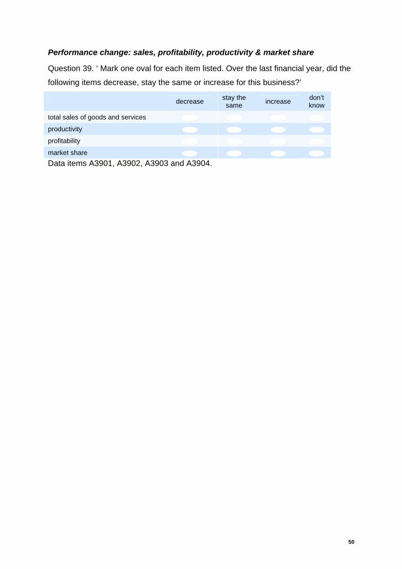
Performance change: sales, profitability, productivity & market share

Question 39. ‘ Mark one oval for each item listed. Over the last financial year, did the

following items decrease, stay the same or increase for this business?’

decrease stay the same increase don’t

know

total sales of goods and services productivity profitability market share Data items A3901, A3902, A3903 and A3904.

50

A1.2 Business Activity Indicator (BAI) Data

The Business Activity Indicator uses GST data from the Inland Revenue Department

matched to the SNZ Business Frame. The BAI data come from the Goods and

Services Tax return form, GST 101. In order to create the BAI dataset, SNZ

temporarily apportion the data down to a monthly frequency, apportion returns across

GST group members and apply limited imputation in cases where a single return

appears to be missing. As noted in Fabling et al. (2008), the GST-based sales and

purchases data is potentially contaminated by capital income and expenditure. In

particular this includes sales of second-hand assets and businesses, purchases of

land, buildings, plant, machinery and businesses. For more on this subject see

section 5.4 of Fabling et al. (2008).

Sales

The sales data in the BAI relate to ‘Total sales and income for the period (including

GST and any zero-rated supplies).’ This is adjusted to an ex-GST basis using data

on zero-rated sales as follows

( ) ZZSS IE +−=98

where SE = Sales excluding GST, SI = Sales including GST, Z = zero rated sales.

In a small number of cases zero-rated GST data is missing. This scenario arises

when GST total sales (and purchases) have been imputed. For these observations,

we assume Z equals zero in the GST adjustment process.

Purchases

The purchases data in the BAI also come from the Goods and Services Tax return

form, GST 101. They relate to ‘Total purchases and expenses (including GST) for

which tax invoicing requirements have been met’ and include an estimate for

imported goods and the use of private goods and services in taxable activity adjusted

by 8/9.

51

A1.3 IR10 Data

The IR10 data used in this paper come from page 1 of the IRD form Accounts

information IR10 form. More information on what should appear in the IR10 form can

be found in the IRD guide IR10G. Note that a table of descriptive statistics for all

items on page 1 of the IR10 is provided in Table 21 of Appendix 2.

Sales

The sales data recorded in the IR10 form relate to Box 2 ‘Gross income from sales

and/or services’ and are GST exclusive.

Other income/revenue

The ‘other income/revenue’ variable used in Table 5 is the sum of Box 7 ‘interest

received’, Box 8 ‘dividends’, Box 9 ‘rental and lease payments’ and Box 10 ‘other

income’.

Profit

The profits data recorded in the IR10 form relate to Box 29 ‘Total current year taxable

profit’. Note that this includes changes in stocks.

Other expenditures

‘Other expenditures’ in Table 5 is the sum of Box 4 ‘Purchases’ (less the change in

stocks from Box 3 ‘Opening stock’ and Box 5 ‘Closing stock’ (both of which include

work in progress)), plus Boxes 13-16, 18, 19, 21-27. For a list of the box numbers,

the names of the variables and descriptive statistics, see Table 21 of Appendix 2.

52

A1.4 LEED/PAYE Data

Our data on employment come from the Linked Employer-Employee Database. It

has two components, counts of employees and working proprietors.

Employees

Employment is measured using an average of twelve monthly PAYE employee

counts in the year. These monthly employee counts are taken as at 15th of the month.

This figure excludes working proprietors and is known as Rolling Mean Employment

(RME).

Working proprietors

The working proprietor count is the number of self-employed persons who were paid

taxable income during the tax year (at any time). In LEED, a working proprietor is

assumed to be a person who (i) operates his or her own economic enterprise or

engages independently in a profession or trade, and (ii) receives income from self-

employment from which tax is deducted.

From tax data, there are five ways that people can earn self-employment income

from a firm:

• As a sole trader working for themselves (using the IR3 individual income tax

form [this is used for individuals who earn income that is not taxed at source]);

• Paid withholding payments either by a firm they own, or as an independent

contractor (identified through the IR348 employer monthly schedule);

• Paid a PAYE tax-deducted salary by a firm they own (IR348);

• Paid a partnership income by a partnership they own (IR20 annual partnership

tax form [this reports the distribution of income earned by partnerships to their

partners] or the IR7 partnership income tax return);

• Paid a shareholder salary by a company they own (IR4S annual company tax

return [this reports the distribution of income from companies to shareholders for

work performed (known as shareholder-salaries)]).

Note that it is impossible to determine whether the self-employment income involves

labour input. For example, shareholder salaries can be paid to owner-shareholders

53

who were not actively involved in running the business. Thus there is no way of

telling what labour input was supplied, although the income figures do provide some

relevant information (a very small payment is unlikely to reflect a full-year, full-time

labour input).

54

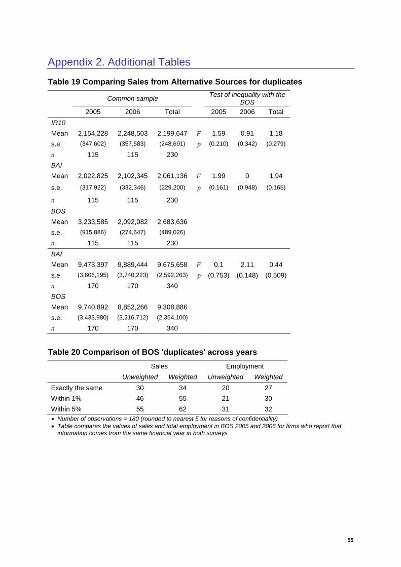
Appendix 2. Additional Tables

Table 19 Comparing Sales from Alternative Sources for duplicates

Common sample Test of inequality with the BOS

2005 2006 Total 2005 2006 Total IR10 Mean 2,154,228 2,248,503 2,199,647 F 1.59 0.91 1.18 s.e. (347,602) (357,583) (248,691) p (0.210) (0.342) (0.279)

n 115 115 230 BAI Mean 2,022,825 2,102,345 2,061,136 F 1.99 0 1.94

s.e. (317,922) (332,346) (229,200) p (0.161) (0.948) (0.165)

n 115 115 230 BOS Mean 3,233,585 2,092,082 2,683,636 s.e. (915,886) (274,647) (489,026) n 115 115 230 BAI Mean 9,473,397 9,889,444 9,675,658 F 0.1 2.11 0.44 s.e. (3,606,195) (3,740,223) (2,592,263) p (0.753) (0.148) (0.509) n 170 170 340 BOS Mean 9,740,892 8,852,266 9,308,886 s.e. (3,433,980) (3,216,712) (2,354,100) n 170 170 340

Table 20 Comparison of BOS 'duplicates' across years Sales Employment Unweighted Weighted Unweighted Weighted Exactly the same 30 34 20 27 Within 1% 46 55 21 30 Within 5% 55 62 31 32 • Number of observations = 180 (rounded to nearest 5 for reasons of confidentiality) • Table compares the values of sales and total employment in BOS 2005 and 2006 for firms who report that

information comes from the same financial year in both surveys

55

Table 21 Page 1 of IR10 Box Number Mean Std. Err. [95% Conf. Interval]

2 Sales and/or goods and services 3,460,763 (96,912) 3,270,784 3,650,7433 Opening stock* 268,903 (12,387) 244,621 293,1864 Purchases 1,872,334 (74,079) 1,727,115 2,017,5535 Closing stock* 285,776 (13,042) 260,209 311,3436 Gross profit 1,605,302 (42,077) 1,522,817 1,687,7877 Interest received 44,312 (10,665) 23,405 65,219

8 Dividends 3,480 (506) 2,489 4,472

9 Rental and lease payments 11,742 (1,219) 9,352 14,13310 Other income 60,634 (5,813) 49,238 72,029 11 Total income 1,725,470 (45,603) 1,636,074 1,814,86612 Bad debts (written off) 4,020 (321) 3,391 4,65013 Depreciation 75,341 (2,513) 70,414 80,26714 Entertainment 2,498 (96) 2,310 2,68515 Fringe benefit tax 3,447 (149) 3,156 3,73816 Insurance (exclude ACC levies) 17,687 (466) 16,773 18,60017 Interest expenses 56,656 (2,859) 51,052 62,26018 Legal expenses 3,057 (206) 2,653 3,46119 Rates 5,972 (356) 5,274 6,67020 Rental and lease payments 101,887 (3,254) 95,507 108,26721 Repairs and maintenance 31,846 (1,378) 29,145 34,54822 Research and development 2,898 (666) 1,591 4,20423 Salaries and wages 608,675 (13,891) 581,445 635,90524 Subcontractor payments 83,705 (9,687) 64,715 102,69425 Travel and accommodation 13,145 (587) 11,994 14,29626 Vehicle (excluding depreciation) 42,501 (1,915) 38,747 46,25527 Other expenses 448,882 (19,492) 410,673 487,092 28 Total expenses 1,502,215 (39,225) 1,425,321 1,579,10929 Total taxable profit 223254.8 11665.7 200386.3 246123.3• * includes work in progress

Table 22 Comparison of unedited IR10 and BOS

Correlation Mean Std. Err. Test of

inequality Spearman Pearson

IR10 3,455,969 98,749 F 3.64 ρ 0.926 0.921 BOS 3,522,878 103,864 p (0.057) p 0 0 • Whole sample (i.e. both years) • n=6,125 (rounded to nearest 5 for confidentiality reasons)

56

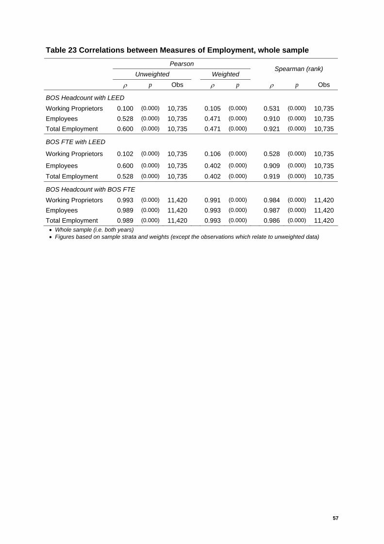
Table 23 Correlations between Measures of Employment, whole sample Pearson Unweighted Weighted

Spearman (rank)

ρ p Obs ρ p ρ p Obs

BOS Headcount with LEED Working Proprietors 0.100 (0.000) 10,735 0.105 (0.000) 0.531 (0.000) 10,735 Employees 0.528 (0.000) 10,735 0.471 (0.000) 0.910 (0.000) 10,735 Total Employment 0.600 (0.000) 10,735 0.471 (0.000) 0.921 (0.000) 10,735

BOS FTE with LEED

Working Proprietors 0.102 (0.000) 10,735 0.106 (0.000) 0.528 (0.000) 10,735

Employees 0.600 (0.000) 10,735 0.402 (0.000) 0.909 (0.000) 10,735 Total Employment 0.528 (0.000) 10,735 0.402 (0.000) 0.919 (0.000) 10,735

BOS Headcount with BOS FTE Working Proprietors 0.993 (0.000) 11,420 0.991 (0.000) 0.984 (0.000) 11,420 Employees 0.989 (0.000) 11,420 0.993 (0.000) 0.987 (0.000) 11,420 Total Employment 0.989 (0.000) 11,420 0.993 (0.000) 0.986 (0.000) 11,420

• Whole sample (i.e. both years) • Figures based on sample strata and weights (except the observations which relate to unweighted data)

57

Table 24 Comparison of unedited BOS with LEED Correlation

Mean Std. Err. Test of inequality Spearman Pearson

2005 Working proprietors n 4,995 BOS (Headcount) 2.14 0.09 F 59.54 31.67 0.072*** 0.539***

BOS (FTE) 1.93 0.09 p (0.000) (0.000) 0.07*** 0.533***

LEED 1.42 0.04 Employees n 5,015 BOS (Headcount) 35.12 4.67 F 2.52 0.26 0.345*** 0.911 BOS (FTE) 30.29 4.57 p (0.112) (0.611) 0.277*** 0.905 LEED 28.03 1.21 Total employment n 4,945 BOS (Headcount) 37.34 4.75 F 3.02 0.4 0.344*** 0.918***

BOS (FTE) 32.28 4.66 p (0.083) (0.529) 0.276*** 0.911***

LEED 29.43 1.22 2006 Working proprietors n 5,230 BOS (Headcount) 1.94 0.06 F 77.5 42.69 0.168*** 0.547***

BOS (FTE) 1.78 0.05 p (0.000) (0.000) 0.185*** 0.546***

LEED 1.39 0.04 Employees 5,410 BOS (Headcount) 29.88 1.33 F 35.1 26.69 0.948 0.91***

BOS (FTE) 25.70 1.11 p (0.000) (0.000) 0.949 0.913***

LEED 27.42 1.12 Total employment n 4,830 BOS (Headcount) 32.32 1.45 F 40.61 13.62 0.946 0.925 BOS (FTE) 28.01 1.22 p (0.000) (0.000) 0.949 0.928 LEED 29.36 1.22 Both years Working proprietors n 10,225 BOS (Headcount) 2.04 0.05 F 127.12 0 0.105*** 0.531***

BOS (FTE) 1.85 0.05 p (68.230) (0.000) 0.106*** 0.528***

LEED 1.41 0.03 Employees n 10,425 BOS (Headcount) 32.46 2.39 F 4.62 0.0316 0.454*** 0.911***

BOS (FTE) 27.96 2.32 p (0.010) (0.912) 0.383*** 0.909***

LEED 27.72 0.83 Total employment n 9,780 BOS (Headcount) 34.92 2.56 F 5.42 0.0199 0.448*** 0.922***

BOS (FTE) 30.23 2.49 p (0.120) (0.724) 0.379*** 0.919***

LEED 29.40 0.86

58

References

Akerlof, G.A., and Yellen, J.L., (1985), ‘Unemployment through the Filter of Memory’,

The Quarterly Journal of Economics, Vol. 100, No. 3, pp. 747-773.

Battistin, Erich, (2003), ‘Errors in survey reports of consumption expenditures’, IFS

Working Papers W03/07, Institute for Fiscal Studies, revised.

Bertrand, M., and Mullainathan, S., (2001), ‘Do People Mean What They Say?

Implications for Subjective Survey Data’, American Economic Review, 91.2,

pp. 67-72.

Bound, John & Brown, Charles & Mathiowetz, Nancy, (2001), ‘Measurement error in

survey data’, in: J.J. Heckman & E.E. Leamer (ed.), Handbook of

Econometrics, volume 5, chapter 59, pages 3705-3843, Elsevier.

Bound, John, and Krueger, Alan B, (1991), ‘The Extent of Measurement Error in

Longitudinal Earnings Data: Do Two Wrongs Make a Right?’, Journal of Labor

Economics, vol. 9(1), pages 1-24, January.

Bradburn, Norman M., (2004), ‘Understanding the Question-Answer Process’, Survey

Methodology, 30, Statistics Canada, pp. 5-15.

Brown, Charles and Medoff, James L., (1996), ‘Employer Characteristics and Work

Environment’, Annales d’économie et de statistique, 41, pp. 219-57.

Cannell, Charles F., Miller, Peter V., and Oksenberg, Lois, (1981), ‘Research on

interviewing techniques’, Sociological methodology, 12, pp. 389-437.

Cochran, WG (1953), Sampling Techniques, New York: John Wiley.

Cooper, A. C., Woo, C. Y., and Dunkelberg, W. C., (1988), “Entrepreneurs’ Perceived

Chances for Success”, Journal of Business Venturing, 3, pp. 97-108.

Cox, V., (2006), ‘IR10 purchases – further analysis’, mimeo, Statistics New Zealand

DeBondt, W.F.M., and Thaler, R.H., (1995), ‘Financial decision making in markets

and firms: A behavioral perspective’, in R. A. Jarrow, V. Maksimovic, and W. T.

Ziemba, (ed.): Handbooks in Operations Research and Management Science,

Volume 9, Finance, pp. 385–410 (Elsevier).

59

Deming, W. E. (1950). Some Theory of Sampling, New York, Dower Publications.

Fabling, R., (2007a), ‘Just how innovative are New Zealand firms? Quantifying &

relating organisational and marketing innovation to traditional science &

technology indicators’, Occasional Paper 07/01, Ministry of Economic

Development, New Zealand. Published as Chapter 10 of Science,

Technology and Innovation Indicators in a Changing World: Responding to

Policy Needs, OECD, Paris.

Fabling, Richard (2007b) ‘Comparison of reported R&D expenditure from BOS’06 &

R&D’06’, Statistics New Zealand mimeo

Fabling, R., and Grimes, A., (2007), ‘Practice makes profit: Business practices and

firm success’, Small Business Economics, 29.4, pp. 383-399.

Fabling, R., and Grimes, A., (2008), ‘Organisational practices and firm performance:

Analysis from a panel of New Zealand firms’, paper presented to Comparative

Analysis of Enterprise Data conference, Budapest.

Fabling, R., Grimes, A., Sanderson, L., and Stevens, P., (2008), ‘Some rise by sin,

and some by virtue fall: Firm dynamics, market structure and performance’,

MED Occasional Paper. 08/01

Fabling, R., Grimes, A., and Stevens, P., (2007), ‘Ask Me No Questions and I’ll Tell

You No Lies: Comparison of Qualitative and Quantitative Firm Performance

Measures’, Presentation to NZAE annual conference, Christchurch.

Forth, J., and McNabb, R., (2008a), ‘Workplace performance: a comparison of

subjective and objective measures in the 2004 Workplace Employment

Relations Survey’, Industrial Relations Journal, 39.2, pp. 104-23.

Forth, J., and McNabb, R., (2008b), ‘The Collection and Validation of Financial

Performance Data in a Workplace Survey, Journal of Official Statistics,

forthcoming.

Hansen, M.H., Hurwitz, W.N. and Madow, W.G. (1953). Sample survey method and

theory. John Wiley and Sons, NY, 456-464.

60

Hillage, J., Regan, J., Dickson, J. and McLoughlin, K. (2002), ‘Employers Skills

Survey 2002’, Research Report 372, London: Department for Education and

Skills.

Horowitz, Joel L., and Manski, Charles F., (1998), ‘Censoring of outcomes and

regressors due to survey nonresponse: Identification and estimation using

weights and imputations’, Journal of Econometrics, Elsevier, vol. 84(1), pages

37-58

Hyslop, Dean R and Imbens, Guido W, (2001), ‘Bias from Classical and Other Forms

of Measurement Error’, Journal of Business & Economic Statistics, 19(4), pp.

475-81

Kneller, Richard and Stevens, Philip A., (2002), ‘The Role of Efficiency as an

Explanation of International Income Differences’, Discussion Paper 205,

London: National Institute of Economic and Social Research.

Knuckey, Stephen and Johnston, Hayden, (2002), Firm Foundations 2002 - A Study

of New Zealand Business Practices and Performance, Ministry of Economic

Development.

Krosnick, J. A., (1991), ‘Response strategies for coping with the cognitive demands

of attitude measures in surveys’, Applied Cognitive Psychology, 5, pp. 213-

236.

Larwood, L., and Whittaker, W., (1977), ‘Managerial Myopia: Self-Serving Biases in

Organizational Planning’, Journal of Applied Psychology, 62, pp. 194-8.

Machin, S., and Stewart, M., (1990), ‘Unions and the financial performance of British

private sector establishments’, Journal of Applied Econometrics, 5, pp. 327-50.

Mason, G., (2005), ‘Enterprise product strategies, high value added production and

employer demand for skills: methodological issues’, mimeo, National Institute

of Economic and Social Research, London.

Mathiowetz, N. (1986). ‘The problem of omissions and telescoping error: New

evidence from a study of unemployment’, Proceedings of the Section on

Survey Research Methods, American Statistical Association.

61

Maré, David C., (forthcoming), ‘Labour productivity in Auckland firms’ Motu Working

Paper/MED Occasional Paper

Poterba, James M and Summers, Lawrence H, (1986), ‘Reporting Errors and Labor

Market Dynamics’, Econometrica, vol. 54(6), pages 1319-38, November.

Prescott, E.C., (1998), ‘Needed: A Theory of Total Factor Productivity’, International

Economic Review, 39(3), pp. 525-552.

SNZ/MED (2005), Business Finance in New Zealand 2004, Statistics New Zealand

and Ministry of Economic Development.

Sudman, Seymour; Bradburn, Norman M., and Schwarz, Norbert (1996), Thinking

about questions: the application of cognitive processes to survey methodology,

San Francisco: Jossey-Bass.

Taylor, S. E., and Brown, J. D. (1988), ‘Illusion and well-being: A social psychological

perspective on mental health’, Psychological Bulletin, II0, pp. 193-210.

Tanur, Judith M., (1992), Questions about questions: Inquiries into the cognitive

bases of surveys, New York: Russell Sage.

Tourangeau, Roger, Rips, Lance J., and Rasinski, Kenneth A., (2000), The

Psychology of Survey Response, Cambridge: Cambridge University Press.

62