a comparison of imputation methodologies in the … comparison of imputation methodologies in the ....

The author(s) shown below used Federal funds provided by the U.S. Department of Justice and prepared the following final report: Document Title: A Comparison of Imputation Methodologies in

the Offenses-Known Uniform Crime Reports Author: Joseph Robert Targonski Document No.: 235152

Date Received: July 2011 Award Number: 2004-IJ-CX-0006 This report has not been published by the U.S. Department of Justice. To provide better customer service, NCJRS has made this Federally-funded grant final report available electronically in addition to traditional paper copies.

Opinions or points of view expressed are those

of the author(s) and do not necessarily reflect the official position or policies of the U.S.

Department of Justice.

A COMPARISON OF IMPUTATION METHODOLOGIES IN THE

OFFENSES-KNOWN UNIFORM CRIME REPORTS

BY

JOSEPH ROBERT TARGONSKI

B.A., University of Colorado at Boulder, 1999

M.A. University of Illinois at Chicago, 2001

THESIS

Submitted as partial fulfillment of the degree requirements

for the degree Doctor of Philosophy in Criminology, Law and Justice

in the Graduate College of the

University of Illinois at Chicago, 2011

Chicago, Illinois

This document is a research report submitted to the U.S. Department of Justice. This report has not been published by the Department. Opinions or points of view expressed are those of the author(s) and do not necessarily reflect the official position or policies of the U.S. Department of Justice.

iii

ACKNOWLEDGEMENTS

I would like to thank that National Institute of Justice for their support of this

research though dissertation fellowship #2004-90721-IL-IJ and the Bureau of Justice

Statistics for their sponsorship of this research during the Quantitative Analysis of Crime

and Criminal Justice Data summer workshop summer workshop at the University of

Michigan.

I would also like to thank my wife, Marianne, for providing motivation and seeing

me though the more stressful times of the research and writing phases.

I am greatly indebted to my committee members Dennis Rosenbaum, Sarah

Ullman, Donald Hedeker, and Joseph Peterson for their support and feedback during all

phases of the research. Most of all, I thank my chairman Michael Maltz, for his countless

hours of mentoring, support, and dedication as my advisor.


iv

TABLE OF CONTENTS

CHAPTER PAGE

I. INTRODUCTION……………………………………………………… 1 A. Statement of the Problem…………………………………………… 1

B. Significance of Imputation…………………………….…………… . 2

C. Research Goals and Objectives……………………………………... 4

D. Chapter Overview…………………………………………………… 5

II. LITERATURE REVIEW………………………………………………. 7

A. History of the Uniform Crime Reports …………………………….. 7

B. Components of the Uniform Crime Reporting Program…………… 9

1. Offenses-Known……………………………………….............. 9

2. Age, Sex, Race and Ethnicity of Arrestees…………………….. 11

3. Supplementary Homicide Reports…………………………….. . 11

4. Law Enforcement Officers Killed or Assaulted …… …………. 11

5. Police Employment……………………………………………. 12

6. Hate Crimes……………………………………………………. 12

7. Nation Incident Based Reporting System …………………….. 13

8. Summary……………………………………………………… 13

C. Coverage of the Uniform Crime Reports ………………………… 14

D. Measurement Error in the Uniform Crime Reports ……………… 14

1. Victim Nonreporting…………………………………………… 14

2. Incomplete Coverage………………………………………….. 15

3. Imputation Issues……………………………………………… 16

4. Hierarchy Rule……………………………………………….. 16

5. Organizational Issues………………………………………… 17

6. Summary……………………………………………………… 18

E. Missing Data and Imputation……………………………………. 18

1. Types of Missing Data……………………………………….. 18

a. Missing Completely at Random…………………………… 19

b. Missing at Random………………………………………. 19

c. Missing Not at Random…………………………………… 20

2. Approaches to Handling Missing Data……………………….. 20

a. Overview………………………………………………… 20

b. Complete case……………………………………………. 21

c. Weighting………………………………………………… 22

d. Single Imputation………………………………………… 22

i. Hot Deck……………………………………………… 23

ii. Mean Substitution……………………………………… 23

iii. Historical/Longitudinal Imputation……………………. 23

iv. Cold Deck………………………………………………. 24

e. Multiple Imputation……………………………………….... 24

F. Simulation Studies……………………………………………….. 25

G. Uniform Crime Reports and Missing Data………………………. 26


v

TABLE OF CONTENTS (continued)

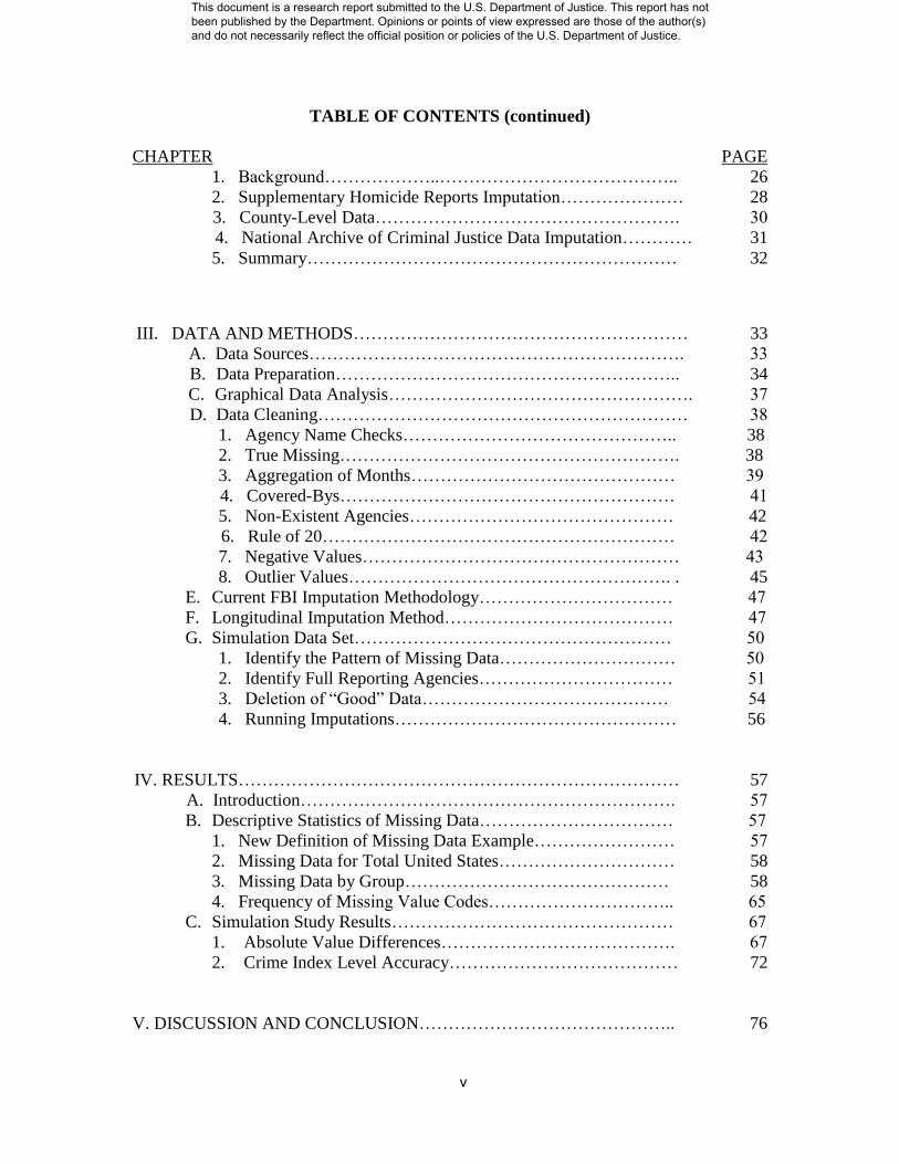
CHAPTER PAGE 1. Background………………..………………………………….. 26

2. Supplementary Homicide Reports Imputation………………… 28

3. County-Level Data……………………………………………. 30

4. National Archive of Criminal Justice Data Imputation………… 31

5. Summary……………………………………………………… 32

III. DATA AND METHODS………………………………………………… 33 A. Data Sources………………………………………………………. 33

B. Data Preparation………………………………………………….. 34

C. Graphical Data Analysis……………………………………………. 37

D. Data Cleaning……………………………………………………… 38

1. Agency Name Checks……………………………………….. 38

2. True Missing…………………………………………………. 38

3. Aggregation of Months……………………………………… 39

4. Covered-Bys………………………………………………… 41

5. Non-Existent Agencies……………………………………… 42

6. Rule of 20…………………………………………………… 42

7. Negative Values……………………………………………… 43

8. Outlier Values………………………………………………. . 45

E. Current FBI Imputation Methodology…………………………… 47

F. Longitudinal Imputation Method………………………………… 47

G. Simulation Data Set……………………………………………… 50

1. Identify the Pattern of Missing Data………………………… 50

2. Identify Full Reporting Agencies…………………………… 51

3. Deletion of “Good” Data…………………………………… 54

4. Running Imputations………………………………………… 56

IV. RESULTS………………………………………………………………… 57

A. Introduction………………………………………………………. 57

B. Descriptive Statistics of Missing Data…………………………… 57

1. New Definition of Missing Data Example…………………… 57

2. Missing Data for Total United States………………………… 58

3. Missing Data by Group……………………………………… 58

4. Frequency of Missing Value Codes………………………….. 65

C. Simulation Study Results………………………………………… 67

1. Absolute Value Differences…………………………………. 67

2. Crime Index Level Accuracy………………………………… 72

V. DISCUSSION AND CONCLUSION…………………………………….. 76


vi

TABLE OF CONTENTS (continued)

CHAPTER PAGE

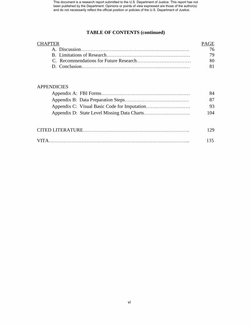
A. Discussion………………………………………………………… 76

B. Limitations of Research…………………………………………… 79

C. Recommendations for Future Research…………………………… 80

D. Conclusion………………………………………………………… 81

APPENDICIES

Appendix A: FBI Forms……………………………………………… 84

Appendix B: Data Preparation Steps………………………………… 87

Appendix C: Visual Basic Code for Imputation……………………… 93

Appendix D: State Level Missing Data Charts………………………. 104

CITED LITERATURE……………………………………………………….. 129

VITA………………………………………………………………………….. 135


vii

LIST OF TABLES

TABLE PAGE

I. MISSING DATA IN THE UNIFORM CRIME REPORTS……… 20

II. FBI GROUP TYPES……………………………………………… 26

III. VARIABLE TYPES ……………………………………………… 35

IV. MONTHLY AGGREGATION MISSING VALUE CODES……. 40

V. SUMMARY OF MISSING VALUE CODES……………………. 46

VI. FREQUENCY OF MISSING VALUE CODES, ALL ORIS,

1977-2000………………………………………………………….. 66

VII. SIMULATION RESULTS OF ABSOLUTE DIFFERENCES……. 69

VIII. SIMULATION RESULTS OF AVERAGE ABSOLUTE VALUE

DIFFERENCES BY RUN LENGTH………………………………. 70

IV. SIMULATION RESULTS OF ABSOLUTE VALUE DIFFERENCES

BY RUN LENGTH…………………………………………………... 71

X. COMPARISON OF CRIME COUNT TOTALS……………………… 73

XI. CRIME COUNT PERCENT ACCURACY TO ACTUAL……………. 74


viii

LIST OF FIGURES

FIGURE PAGE

Figure 1. FBI Algorithm for Imputation……………………………… 27

Figure 2. Variable Naming…………………………………………… 34

Figure 3. Quarterly, Semiannual and Annual Reporting Example…… 39

Figure 4. Rule of 20………………………………………………… 43

Figure 5. Negative Crime Values, 1977-2000……………………….. 44

Figure 6. Outlier 9999 Value for Crime Index, Durango, CO………. 45

Figure 7. Longitudinal Imputation Example………………………… 49

Figure 8. Missing Data Run Lengths for All ORIs………………….. 50

Figure 9. Number of ORIs that Qualify for Imputation by State……. 53

Figure 10. Percent of ORIs that Qualify for Imputation by FBI Group.. 54

Figure 11. Screenshots of Simulated Data…………………………… 55

Figure 12. Percent of Missing Data All ORIs…………………………. 58

Figure 13. Percent of Missing Data Group I…………………………… 59

Figure 14. Percent of Missing Data Group II………………………….. 60

Figure 15. Percent of Missing Data Group III…………………………. 61

Figure 16. Percent of Missing Data Group IV…………………………. 61

Figure 17. Percent of Missing Data Group V………………………….. 62

Figure 18. Percent of Missing Data Group VI…………………………. 62

Figure 19. Percent of Missing Data Group VII…………………………. 63

Figure 20. Percent of Missing Data Group VIII………………………… 64

Figure 21. Percent of Missing Data Group IV………………………….. 64

Figure 22. Comparison of Crime Count Totals………………………… 73


ix

Figure 23. Yearly Differences of Imputation Methods for Total US Base on the

average of the five iterations……………………………………… 75


x

LIST OF ABBREVIATIONS

CIUS Crime in the United States

FBI Federal Bureau of Investigation

IACP International Association of Chiefs of Police

ICPSR Inter-university Consortium for Political and Social Research

LOCF Last Observation Carried Forward

LEAA Law Enforcement Assistance Administration

LEOKA Law Enforcement Officers Killed and Assaulted

MAR Missing at Random

MCAR Missing Completely at Random

MI Multiple Imputation

MNAR Missing Not at Random

NACJD National Archive of Criminal Justice Data

NCIC National Crime Information Center

NPA National Police Association

NVSS National Vital Statistics System

NCVS National Crime Victimization Survey

NIBRS National Incident Based Reporting System

ORI Originating Agency Identifier

SAC Statistical Analysis Center

SHR Supplementary Homicide Reports

SPSS Statistical Package for Social Sciences

SSLEA Sample Survey of Law Enforcement Agencies

UCR Uniform Crime Reports


xi

VBA Visual Basic for Applications


xii

SUMMARY

One of the most widely used and important sources of crime data for

criminologists and criminal justice policy stakeholders is the Offenses-Known Uniform

Crime Reports (UCR). However, it comes with many limitations, including missing data

from non-compliant police agencies. The missing data are adjusted for by imputing data

based on a cross-sectional methodology to maintain comparable trending analysis.

The purpose of this study was to reexamine and recode missing data in the UCR

for the years 1977-2000 for all police agencies in the United States. With the newly

cleaned dataset, a clearer picture of the UCR error structure would emerge and patterns of

missing data could more accurately be described. The study found that there are more

missing data than identified by the FBI’s quality control.

The next phase of the project was to create a dataset with only full reporting

agencies for a 10 year period, which would be used to test the cross-sectional method

against a longitudinal method. This was done by creating simulation data sets that

“punched out” the real crime values, thus artificially creating missing data. Each

imputation method could then be tested by comparing the imputed value to the actual

value. The overall results showed that in most circumstances, the longitudinal method

was more accurate at estimating the missing crime data points.


1

I. INTRODUCTION

A. Statement of the Problem

Academics, researchers, police chiefs, and policy analysts make extensive use of

the FBI’s Offenses-Known Uniform Crime Report (UCR) data. While these data are

routinely used for important research and policy decisions, there are many gaps in the

data that are filled in based on an imputation methodology developed in the 1950’s when

computing and data storage capabilities were limited. Although it is the nation’s primary

source for crime data, it has many weaknesses. The weakness most researchers have

focused on is the so-called “dark figure” of crime, or crimes that are not reported to the

police (Skogan 1977). While the UCR is a census of law enforcement agencies, that does

not mean it is immune from the problem of non-compliance and missing data. This is an

issue that has become more pronounced over time as funding and resources have been

reduced for law enforcement agencies to support their UCR reporting (Maltz 1999).

Since 1958, the FBI has used an untested method to impute, or filled in the

missing data for its yearly report, Crime in the United States. This method is based on

cross-sectional data, which does not account for an agency’s past reporting history, or

issues such as seasonality and zero population jurisdictions. This dissertation will seek to

1) Identify the nature and extent of missing data in the Offenses-Known UCR, 2)

Develop methods to clean the FBI’s dataset, and 3) Test the FBI’s current imputation

methodology against an alternative longitudinal imputation method.


2

B. Significance of Imputation in the UCR

Generating the UCR takes a great deal of time and effort, not only for the FBI, but

for the over 17,000 police agencies that collect and transmit data their crime data to the

FBI1. Considering the resources used in this endeavor, it is unfortunate that so little use

is made of the data. In fact, they are used primarily to provide state, regional, and national

trends. For this purpose, the current cross-sectional method of imputation was adequate.

However, in recent years the uses of UCR data have expanded. UCR data sets are now

more accessible since they are on the internet, the UCR has been used in determining

allocation of federal funds, and researchers are using the data for smaller geographic units

(Maltz 1999).

At the county level, UCR data have been used to investigate a number of policy-

related issues (Wilkinson 1984; Petee and Kowalski 1993; Petee, Kowalski et al. 1994;

Kposowa, Breault et al. 1995). Several studies have recently examined the relationship

between “right-to-carry” laws and violent crime using county-level data (Lott and

Mustard 1997; Lott 1998; Lott 2000). Lott’s books not only opened up research into the

effect of these laws, it had the side benefit of popularizing county-level crime data in

general. When examining crime rates at the county-level, imputation becomes even more

important because those estimates are much more sensitive to missing data.

These county-level studies used either the FBI’s annual “Crime by County” data

sets or the annual county-level crime data set from the National Archive of Criminal

Justice Data (NACJD) – which is based on the FBI’s Crime by County file. Both of these

1 Some police agencies report their data first to a state-level agency


3

data sets have major flaws that are detailed in Maltz and Targonski (2002, 2003). That is,

the imputation strategies used by both the FBI and NACJD have significant deficiencies.

With the advent of the internet, UCR data are being used more extensively. The

results of any study of criminal justice policy that uses UCR data will only be as robust as

the data it uses. However, as criminal justice researchers increasingly use UCR data for

complex statistical studies, and at smaller and smaller levels of aggregation, there is a

stronger need for a more sophisticated imputation method.

As noted above, the UCR has been used for the appropriation of federal anti-

crime funding. This occurred with the with 1994 reauthorization of the Omnibus Crime

Control and Safe Streets Act of 1968. Funding to local agencies was allocated based on

the number of violent crimes in the prior three years, using the unimputed data in the

UCR. Maltz (1999) found that for the three years of data that was being used to

disseminate these funds, 19% of police agencies did not provide even a single month of

data. Such major federal policy decisions need to be made on the most accurate and

reliable data possible. When police agencies fail to report their data to the FBI,

scientifically sound imputation methods are the only way to make up for the missing

values. As the UCR becomes more important in federal policy decision-making and fund

allocation, the methods used to impute for missing data become even more critical.

The UCR is not the only criminal justice-related data source where imputation is a

major factor. Imputation has also been an important issue in studies using the National

Crime Victimization Survey (Ybarra and Lohr 2002) and the Sample Survey of Law

Enforcement Agencies (SSLEA) (Dorinski 1998). Imputation is useful in government


4

surveys because it allows for the creation of complete rectangular datasets that can easily

be analyzed by researchers (Little 1988).

Given the importance of UCR data, many police chiefs and politicians have

succumbed to manipulating the data for political gain. Examples have been documented

of data tinkering in the District of Columbia and Philadelphia where offenses were

downgraded to keep them out of the crime index (Seidman and Couzens 1974), and

Maltz (1999) documented this practice in other cities. Most often, the manipulation is

downward. Police and politicians want to show they are “doing something” about crime

and that the result of their efforts is a reduced crime index.

C. Research Goals and Objectives

The purpose of this project is to develop a more accurate and reliable method of

imputing crime data in the Uniform Crime Reports (UCR) and to provide a more

complete understanding of UCR missing data and error structure. This will be

accomplished by the following steps:

1) A thorough data cleaning of approximately 17,000 ORIs based on the

Offenses-Known UCR data from 1977 to 2000. It is based on an agency-level data set

that includes all Originating Agency Identifiers (ORIs), which are the FBI identification

codes for individual police agencies in the UCR system. This single data set includes all

the crime data on a monthly basis between 1977-2000 for each police agency. It includes

whether or not each month was reported, based upon the FBI definition of a missing data

point and the quality control parameters designated by the researchers. In addition, it

includes a host of new numerical codes for different types of missing data.


5

2) Analysis of this cleaned dataset, to provide insight to the types of data

errors and patterns of missing data in the UCR.

3) Development of a “simulation dataset” based on ORIs with complete

reporting for data ten-year period. This complete reporting file will then have some of

the real data points selectively deleted or also referred to as “punched out”. That will

allow the “real” values to be compared to the estimated values from both the current FBI

imputation method and the longitudinal method.

As with any secondary analysis, this study is limited to the quality and

completeness of the available data. The researcher did not have any involvement in the

collection or original cleaning of the data. In the case of the UCR, many studies have

examined the weakness of the data and limitations of its use. These weaknesses will be

described in greater detail in the literature review.

For the data cleaning that was done for the project, all the analysis was done on

the data as archived. Follow-up or input was not derived from the reporting agencies

through any phone calls or in-person interviews. Given the scope of the project and the

thousands of ORIs involved, such follow-up was not feasible.

D. Chapter Overview

Chapter two provides a comprehensive review of the literature. This includes the

history of the UCR system, prior research on UCR weaknesses, and an overview of

various imputation methods. Chapter three explains the methods used, including the

sources, data cleaning steps, and new missing value codes. Chapter four describes the

missing data in the UCR and the basis for the imputation dataset. Chapter five provides


6

the results of the two imputation methods based on the simulation dataset. Chapter six

includes the discussion and recommendations for future research on UCR imputation.


7

II. LITERATURE REVIEW

A. History of the UCR

The Uniform Crime Reporting (UCR) system was developed in 1929 by the

International Association of Chiefs of Police (IACP), which was originally the National

Police Association (NPA) (Maltz 1977). At that time, there was no national collection of

criminal statistics. The goal was to produce a data collection system that would have

uniform definitions for crime and allow for cross-jurisdiction comparison. A crime data

collection system would also provide a way to measure crime and would counter the

efforts of journalists who would manufacture crime waves to sell newspapers (Maltz

1977). Several different methods of crime measurement were proposed, but ultimately

the committee decided on measuring crimes recorded by the police. After consulting

local police departments, a list of seven crimes, now known as the Crime Index or Part I

crimes, were chosen. These seven crimes include murder, rape, robbery, assault,

burglary, larceny and auto theft and still function as the Crime Index today2. They were

chosen based on the fact that they were serious, prevalent and likely to be reported.

In addition to the Index Crimes, the UCR program began collecting data on lesser

offenses where are referred to as the “Part II” crimes. Part II crimes include simple

assault, fraud, vandalism, disorderly conduct and gambling3. The responsibility for

collection and publishing the data became the task for the Bureau of Investigation, later

known as the Federal Bureau of Investigation (FBI).

2 Arson was added to the UCR in 1979, which became known as the Modified Crime Index. The Standard

Crime Index is still reported without arson. The arson data was not included for this research project. 3 For a complete list and detailed description of Part II crimes, see the Uniform Crime Reporting Handbook

(FBI 1984)


8

In the first two years of 1930 and 1931, the FBI published the crime data on a

monthly basis. Over time, this was reduced to quarterly in 1932, semiannually in 1943

and finally went to annual reporting in 1958.

The UCR program did not receive a major overhaul until 1958. In the prior year, a

committee was formed to evaluate the UCR program and recommend changes (FBI

1958). In addition to only releasing data annually, the committee recommended a

number of changes to the way data were reported in the Crime Index. Negligent

manslaughter was excluded, as were larcenies under fifty dollars, statutory rapes and

simple assaults (FBI 1958). The biggest change related to this research was that the FBI

began its imputation method that is still applied today4.

Through the 1960’s and 1970’s, the burden of collecting local agency data shifted

to the states, which would serve as an intermediary between the local agencies and the

FBI’s UCR program. The rise in state-level agency reporting was directly related to

funding by the Law Enforcement Assistance Administration (LEAA), which provided

funding for states to develop Statistical Analysis Centers (SACs). Many states have the

SACs serve as the clearinghouse for state-level UCR data, but some states delegate this

task to their State Police. In 1999 there were 44 states that had state-level reporting

agencies that met the FBI’s requirements (Maltz 1999). However, of these 44 states, only

25 had state-level laws requiring their local police agencies to report their crime data

(Riedel and Regoeczi 2004).

4 This will be discussed in greater detail in Chapter four.


9

In 1985, the FBI commissioned a study called Blueprint for the Future of the

Uniform Crime Reporting Program (Poggio 1985) , which outlined long-term changes to

crime reporting in the United States. The focus of this report was shifting the system

from the summary Crime Index to an incident-based system, now called the National

Incident Based Reporting System (NIBRS). This would provide detailed victim,

offender, and weapon information at the incident level for each crime recorded by the

police. South Carolina was the first state to be NIBRS-compliant and as of 2007, 31

states are compliant, representing 6,444 police agencies (FBI 2011).

B. Components of the Uniform Crime Reporting Program

1. Offenses-Known

The primary data collection system of the UCR is the Offenses-Known data,

which collects monthly crime tabulations. They are collected on what is known as the

“Return A5” form, which is submitted monthly

6 by police agencies. This includes the

Crime Index, which encompasses murder, rape, robbery, aggravated assault, burglary,

larceny, and motor vehicle theft (and arson, see Note 1). Part II offenses, which include

lesser offenses such as gambling, liquor law violations, and prostitution are also collected

but are not included in the official crime index. Data are collected on clearances of

crimes providing an indication of the effectiveness of police investigations. The Return

A also asks for data on “unfounded crimes,” or incidents that are found to be false or

baseless.

5 For examples of the Return A and Supplementary Homicide Report forms, see Appendix A.

6 While a majority of agencies report monthly data per the FBI guidelines, some jurisdictions report

quarterly, semiannual, or annual data. This will be described in greater detail in chapter three.


10

There is also the Supplement to the Return A, which collects information on value

and type of property stolen and property recovered by the police. It also includes

breakdowns of offenses such as the location of robberies, time and location of burglaries,

and types of larceny.

An important step in tabulating the Offenses-Known data is the hierarchy rule.

For each crime incident, no matter how many offenses are committed, only the most

serious offense is to be counted on the Return A (FBI 1966; FBI 1984). The hierarchy

rule is eliminated under NIBRS, which will be discussed in greater detail later.

Once submitted to the FBI, the data undergo scrutiny for reporting accuracy. The

FBI looks for sharp rises or drops in crime trends to assess the accuracy of the data.7 If

they find problems with the data, follow-up procedures are implemented as a quality

control feature. The FBI holds training seminars for police departments on UCR

reporting and provides them with the Uniform Crime Reporting Handbook (FBI 1984)

that gives a detailed explanation of reporting procedures.

Once all the data are in, the FBI analyzes the data to assess crime trends. They

also compute a crime rate, which is the number of crimes divided by the population of a

given area. Each year, the FBI publishes Crime in the United States, which provides a

detailed breakdown of police crime data to the public. The data from the UCR are also

electronically archived for researchers to analyze.

7 However, not all of the data anomalies are caught by the FBI.


11

2. Age, Sex, Race and Ethnicity of Arrestees (ASR)

Arrest information is captured on the age, sex, race and ethnicity of offenders.

This information is also collected monthly and is divided into adults and juveniles under

the age of 18. Arrest information is collected for Part I and II crime, as well as curfew

and runaway information for juveniles.

3. Supplementary Homicide Reports (SHR)

In addition to the summary homicide counts on the Return A, additional data are

collected via the Supplementary Homicide Reports (SHR), which was added to the UCR

system in 1961. The SHR is incident- rather than summary-based. The SHR collects

additional data on each homicide, including information on the victim/offender

relationship; age, sex, and race of victim and offender (if known); weapons; circumstance

of the homicide8, and situation

9. Coverage was minimal in the early years of the system,

with data primarily coming from larger cities (Riedel 1990). The detailed information

provides a rich description of homicide, which cannot be extracted from summary data.

However, the SHR is not without its limitations. Problems have been identified with the

coding of circumstances (Loftin 1986) and with missing data (Maltz 1999; Fox 2000).

4. Law Enforcement Officers Killed and Assaulted (LEOKA)

The FBI also collects information on police officers killed or assaulted in the line

of duty. Law Enforcement Officers Killed and Assaulted (LEOKA) program collects

data on a monthly basis for such incidents, along with details on the weapons used, type

8 Examples of circumstances include rape, robbery, burglary, arson, prostitution, gambling, lover’s triangle,

argument over money, gangland killing, youth gang killing, sniper attack and unknown. 9 Situations include Single Victim/Single Offender, Single Victim/Unknown Offender/Offenders, Single

Victim/Multiple Offenders, Multiple Victims/Single Offender, Multiple Victims/Multiple Offenders,

Multiple Victims/Unknown Offender or Offenders.


12

of assignment, time of day, circumstance, as well as a text based narrative. The system

also collects information on the circumstances related to officers killed or assaulted and

arrest attempts. It includes details on assignment type, weapon used, and type of police

activity

5. Police Employment

On an annual basis, the UCR program collects data on law enforcement

employees. This provides details on number of officers, number of civilian employees,

and gender composition.

6. Hate Crime

In the 1980’s, the term “hate crime” was originally coined by Congresspersons John

Conyers, Barbara Kennelly, and Mario Biaggi in the first appearance of the bill that

would mandate federal collection of data on bias-motivated crime (Jacobs and Potter

1998). This led to increased usage of the phrase in the media to refer to crimes that were

motivated by racial/ethnic or religious prejudice. The bill passed and became known as

the Hate Crime Statistics Act of 1990.

Among the reporting states, each of their own statutes differs as to what constitutes a

hate crime. To avoid this problem, the FBI has its own criteria that are used to

standardize reporting. The FBI statute includes bias motivated crime for race, religion,

disability, sexual orientation, or ethnicity/national origin and is defined as, “A criminal

offense committed against a person or property which is motivated, in whole or in part,

by the offender’s bias against a race, religion, disability, sexual orientation, or

ethnicity/national origin; also know as a Hate Crime (FBI 1999).”


13

The incident level portion of the Hate Crime statistics reporting includes additional

information on each incident, including type of bias, victim information, number of

victims, and race and number of offenders.

7. National Incident-Based Reporting System (NIBRS)

While the summary UCR statistics provide an aggregate-level view of crimes

reported, it provided little detail on individual crime incidents. To enhance the reporting

of police crime statistics, the FBI developed the next generation of the UCR program

with the National Incident-Based Reporting System (NIBRS). It is based on the

guidelines and recommendations of the aforementioned report (Poggio 1985), it provides

incident-level crime reporting, rather than only the summary reports found on the Return

A. There are a number of other changes from the summary UCR, as described in (FBI

2000):

Updated crime definitions

Forcible rape could include male victims

Abolition of the hierarchy rule

Details on victim and offender characteristics

Data on crimes against society (drug crimes, gambling, prostitution, etc)

8. Summary

Although the FBI collects all these various data sets, the one that is used and cited

most frequently is the Crime Index, or Offenses-Known data. When journalists,

politicians, or criminologists refer to police crime data or the crime rate, they are most


14

often talking about the Part I Crime Index. As the data for the project focused on the Part

I index crime, all references to “UCR” will pertain to the Offenses-Known segment of the

UCR program.

C. Coverage of the UCR

The UCR encompasses all state and local law enforcement agencies, which

submit data on a voluntary basis. The UCR is not a sample of agencies, but attempts to

gather data from every state and local police agency. It attempts to take a census of law

enforcement agencies, but is actually a “pseudo-census” because some members of the

population are not reached (Maisel and Persell 1996). Each police agency is given an

Originating Agency Identifier (ORI) code that is assigned by the FBI. The FBI originally

began using the ORI code to identify agencies with computer terminal linked to National

Crime Information Center (NCIC).

D. Measurement Error in the UCR

1. Victim Nonreporting

One of the greatest weakness is of the UCR is that it only counts crimes that are

reported to the police (Skogan 1974; Skogan 1975; Skogan 1977; Schneider and

Wiersema 1990; Mosher, Miethe et al. 2002). Crimes that occur but are not brought to

the attention of the police are referred to as the “dark figure” of crime. Sometimes crimes

such as shoplifting may go completely undetected (Schneider and Wiersema 1990).

Moreover, many citizens that either are victimized or witness a crime fail to report

it. Many factors influence citizen reporting of crimes to the police. Thinking the police

can do very little, lack of confidence in the police, and not knowing the procedures to


15

report a crime may prevent a victim from reporting a criminal incident (Schneider and

Wiersema 1990). Other studies have found that citizens are more likely to report a crime

to the police if they had positive police interactions in previous victimizations that had

been reported (Conaway and Lohr 1994), however, police do not always have a good

track record of handling the psychological needs of victims (Rosenbaum 1987). Rape is

one of the most underreported crimes, which is due to several factors. Rape is an

emotionally disturbing crime, and victims often experience symptoms of posttraumatic

stress (Ullman and Siegel 1994). The victim may even have to convince herself that

she10

was victimized before she feels she can convince others (LaFree 1989).

Victim surveys, particularly the National Crime Victimization Survey (NCVS),

data can be used as a comparison to measure the level of unreported crime to the police.

Only 36.8% of all victimizations are reported to the police, with rates as low as 30.7% for

rape and 28.4% for larceny (Ringel 1997). While the NCVS shows a clear level

difference in the amount of crime compared to the UCR, the evidence is more mixed on

whether the two systems agree or disagree on the trend in crime. Some researchers argue

that the two systems trend similarly (O'Brien 1990; O'Brien 1991; Blumstein, Cohen et

al. 1992) while others argue they do not (Menard 1991; Menard 1992). For a complete

analysis of the UCR-NCVS trending debate, see Lynch and Addington (2007).

2. Incomplete Coverage

Federal collection of crime data has always had the problem of non-compliance

by police departments. Claims of high reporting participation in the UCR are often

10

While under many state statutes men can be victims of rape, the FBI UCR definition specifies that the

victim is a woman.


16

misleading, since an agency may be considered “participating” if it submits only one

month of data for the entire year. Given the voluntary nature of the UCR program, the

FBI does not have much leverage to get agencies to report their data.

The most comprehensive analysis regarding the extent of coverage and missing

data in the UCR is found in Maltz (1999). Maltz found that UCR coverage had decreased

over time, with less of the population being covered often due to the agencies’ problems

with conversion to NIBRS. In addition, factors such as budgetary constraints and natural

disasters impede the ability of police agencies to keep accurate records of crime11

. There

is also a wide disparity between states, with states such as Illinois submitting

unacceptable data resulting from state law defining rape in a gender-neutral way, while

the FBI defines it as forcible intercourse between a man and a woman.

3. Imputation Issues

In the case of missing data, the FBI imputes data using a cross-sectional method.

The imputation is only used for state and national estimates of crime and is not reported

for individual agencies. The National Archive of Criminal Justice Data (NACJD)

produces an imputed county-level dataset, which began with a different imputation

method, and which has been criticized for undercounting crime in many counties (Maltz

and Targonski 2002; Maltz and Targonski 2003).

4. Hierarchy Rule

11

It is yet to be determined how state and municipal budget problems will impact crime reporting. Some

cities have begun reductions in staffing for police agencies, most notably Newark, NJ, which has recently

considered eliminating over 200 police positions (Queally and Giambusso 2010)


17

The hierarchy rule provides another source of measurement error and under

coverage. Since only the most serious offense is recorded in an incident, the crime rate

will be biased downward. Related to the hierarchy rule is the “hotel rule.” If a series of

burglaries occurs in a dwelling with multiple residences, the burglary is scored as one

offense rather than multiple (FBI 1984). The hotel rule does bias burglary rates because

not all cities have the same proportion of transient or multi-family housing. For example,

resort areas would have a burglary rate biased downward as compared to an area with

primarily single-family homes.

5. Organizational Issues

Organizational issues can also influence police crime reporting (Kituse and

Cicourel 1963; McCleary, Nienstedt et al. 1982). Police are decision makers, and factors

such as complainant’s social class and attitude toward the police have been found to

influence crime reporting (Black 1970). Police turnover and organizational change can

influence rates of reported crime. One study found that burglary rates can be influenced

by changes in police management, making the crime rate more a function of

organizational goals rather than an accurate measure of crime (McCleary, Nienstedt et al.

1982). Problems can also arise at the state reporting level, with overworked clerks unable

to give the proper time for quality control (Brownstein 2000). The way crimes are

classified and scored is also subject to measurement error. Misclassification of crimes,

particular simple and aggravated assault, has been identified as an issue with UCR

reporting (Nolan, Hass et al. 2006).


18

Technological advancement can aid the process, but it can also be a hurdle. For

example, conversion to NIBRS has disrupted summary UCR reporting in Vermont, New

Hampshire, and Kansas (Maltz 1999).

6. Summary

Although the UCR is the primary source of data on crime, it does have many

weakness and limitations. While some limitations are inherent to measuring crime from

police reports, imputation is an area that researchers and the FBI have some control over.

Testing and enhancing imputation methods are an important part of criminal justice

research with UCR data that should not be overlooked.

E. MISSING DATA AND IMPUTATION

1. Types of Missing Data

Despite the best efforts of researchers, almost all datasets have missing data. The

UCR and all criminal justice data are no exception. Whether it is UCR data or another

source of crime data, criminologists too often rely on complete-case analysis as an

approach to handling missing data (Brame and Paternoster 2003). This section will seek

to summarize the different methods researchers have developed to handle missing data

and how these methods have been applied to crime data.

When assessing and analyzing missing data trends, it is important to consider the

missing data mechanisms. The underlying cause of the missing data can have an

influence on which type of imputation method is selected. The three types of missing

data, also referred to as “missingness,” are described as being missing completely at


19

random (MCAR), missing at random (MAR), and missing not at random (MNAR) (Little

and Rubin 1987; Rubin 1987).

a. Missing Completely at Random (MCAR)

Data can be classified as missing completely at random when the probability of

missing data for variable X is unrelated to itself or another other covariates in the data

set. Thus, missing data are not correlated with any of the variables in the data set. This

can be the most easily adjusted for type of missing data and is ideally suited for multiple

imputation techniques (Little and Rubin 1987). Hypothetically, even listwise deletion

would yield reliable results, because the complete cases would statistically be no different

than the missing cases. However, the criteria for MCAR are difficult to meet because

data are often correlated with other factors.

In the case of the UCR, an ORI’s data could be considered MCAR only if the data

were missing for some reason unrelated to crime, such as a natural disaster that prevented

the agency from submitting UCR reports (Maltz 2007).

b. Missing at Random (MAR)

Data are Missing at Random (MAR) when the probability of missing data on a

variable is non-random only in the bivariate case for measured variables. An example in

homicide data is where the circumstance variable could be MAR if it was related to the

victim-offender relationship, but not the circumstance itself (Wadsworth, Roberts et al.

2008).

Maltz (2007) identifies computer problems and noncompliance with UCR

standards and examples of MAR for UCR data. Computer problems with UCR reporting


20

stemmed from conversion to the National Incident Based Reporting System (NIBRS).

Some cities encountered software issues in the conversion, which left them without any

way to report via NIBRS or the summary UCR system.

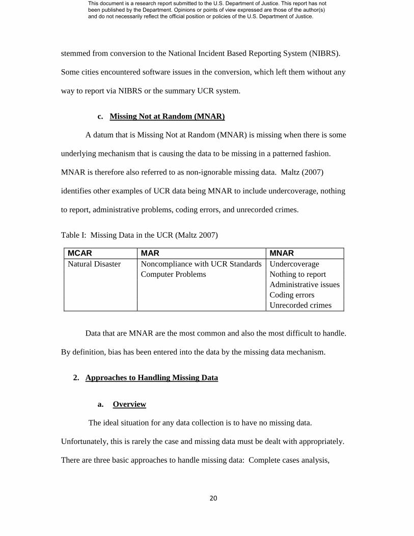
c. Missing Not at Random (MNAR)

A datum that is Missing Not at Random (MNAR) is missing when there is some

underlying mechanism that is causing the data to be missing in a patterned fashion.

MNAR is therefore also referred to as non-ignorable missing data. Maltz (2007)

identifies other examples of UCR data being MNAR to include undercoverage, nothing

to report, administrative problems, coding errors, and unrecorded crimes.

Table I: Missing Data in the UCR (Maltz 2007)

MCAR MAR MNAR

Natural Disaster Noncompliance with UCR Standards Undercoverage

Computer Problems Nothing to report

Administrative issues

Coding errors

Unrecorded crimes

Data that are MNAR are the most common and also the most difficult to handle.

By definition, bias has been entered into the data by the missing data mechanism.

2. Approaches to Handling Missing Data

a. Overview

The ideal situation for any data collection is to have no missing data.

Unfortunately, this is rarely the case and missing data must be dealt with appropriately.

There are three basic approaches to handle missing data: Complete cases analysis,


21

weighting, and imputation. Each has its own pros and cons and is most appropriate

depending on the type of data and type of missingness.

b. Complete Case Analysis

When faced with missing data, researchers face several options to adjust for the

missing cells. The first approach is to ignore the cases with missing values and only

analyze cases with no missing data, known as complete case analysis. Canned software

packages will sometimes default to this method using what is called listwise deletion.

Only cases that have every cell accounted for are kept for analysis. Of course, this

introduces a bias into the analysis if the cases with missing data are not representative of

the cases with complete data.

An example of this bias is identified by Maltz and Targonski (2002), which

critiqued the methodology of More Guns, Less Crime (Lott 1998; Lott 2000). Using an

example from Delaware County, Indiana, Maltz and Targonski show how the NACJD

imputation methodology excluded the crime estimate for the ORIs, which led to a

downward bias in the crime rate for that county. Delaware County was not an isolated

example and some states had over half of their county-level data points with population

coverage gaps of 30% or more. In addition, the states with the most missing data were

skewed toward states that had more permissive right-to-carry guns laws, which

introduces bias into evaluating the effect of those laws.

While this complete case analysis is very simple and yields only cases with

complete data reporting, there are several drawbacks. If there is only a small amount of

missing data and it is MCAR, listwise deletions may not have a severe impact on the


22

results. However, as the number of missing data increases, fewer and fewer cases will be

included for analysis. If these cases are either MAR or MNAR, more bias is introduced

into the results. In addition, this is a very unforgiving method of handling missing data.

In a large dataset with dozens of variables, listwise deletion will discard the entire case

when it is missing only one of the variables. This is particularly true for longitudinal

datasets with multiple waves of data, which increases the chances that at least one of the

waves will be missing or incomplete.

b. Weighting

Weighting procedures are typically applied to larger amounts of missing data,

such as unit nonresponse. The Supplementary Homicide Reports (SHR) use a weighting

technique for both the victim and offender files (Maltz 1999; Fox 2004). Weighting

methods work by applying a weight value to the non-missing cases to account for the

missing cases. This is preferable to complete case analysis, but should only be applied to

monotone patterns of missing data (Little and Rubin 1989).

It is important to note that the goal of imputation is to make inferences about an

aggregate population, not to estimate or predict missing data for incomplete cases

(Schafer and Graham 2002). Using the UCR as an example, the objective of imputation

should be to attain national, state, and county crime estimates, not to predict the missing

cells for incomplete reporting ORIs. Therefore, imputations at the ORI level should not

be released as representing crime for that jurisdiction.

c. Single Imputation

i. Hot Deck


23

In hot deck imputation, missing values are borrowed from a “donor” case that

most closely matches the missing case. The name traces its origins to the days of data

processing when information was stored on cards and sorted in a manner that similar

cases were clustered together. Hot deck can be performed using the “nearest neighbor”

or on a set of independent variables that attempts to most closely match cases. Hot deck

imputation is most appropriate for categorical variables or when there is substantial

missing data (Yansaneh, Wallace et al. 1998). Hot deck imputation has been used to

impute for the population census (Lillard, Smith et al. 1986) and has also been proposed

in SHR imputation (Fox 2004).

ii. Mean Substitution

Perhaps the most basic of imputation methods is mean substitution, whereby the

mean value for all reporting cases is imputed for the missing case. The advantage to this

method is that it is very simple and straightforward to implement. However, it has its

obvious drawbacks, in particular skewing the distribution to concentrate values and create

abnormal distributions. Thus, this method typically yields statistically invalid estimates

(Rubin 1996).

iii. Historical/Longitudinal Imputation

Longitudinal imputation is a method whereby in a longitudinal dataset, data from

prior responses of the same respondent (or case) is used to impute for the missing value.

This method is also referred to as historical imputation, since it uses the past reporting

history for a particular respondent. The most basic form of this method is known as Last

Observation Carried Forward (LOCF). LOCF is where the most recent historical value is


24

imputed for the missing value. For example in the UCR, if the Chicago Police

Department was missing data on assault for December 2006, the assault data for Chicago

in December 2005 would be substituted for the missing December 2006 value. This

method has been used for the Sample Survey of Law Enforcement Agencies (SSLEA)

(Dorinski 1998). The strength of this method is that a respondent’s data are imputed

from a respondent’s own data, rather than trying to infer from similar cases. The

downside is a decrease in variance, since the same datum is carried forward from wave to

wave. A method that incorporates both a longitudinal and cross-sectional imputation

methods was developed by Little and Su (1989). The strength of this method is that it

can incorporate the influence of the individual and the trend of similar cases.

iv. Cold Deck

Unlike hot deck, cold deck imputes values from a different dataset. Often, this is

a datum that was collected as part of a previous wave or similar survey. When a datum is

used from a previous wave, the method is also a variation of historical imputation, since

it derives the imputed value based on previously collected data.

d. Multiple Imputation

The methods described above can be classified as single imputation techniques,

because the resulting dataset will contain a single value for the missing data points. An

alternative method is multiple imputation (MI), which creates multiple possible values

per missing data point (Little and Rubin 1987; Rubin 1987; Rubin 1996). The number of

required iterations differs, but the more incomplete the dataset the more iterations that


25

will be required. Each iteration produces a complete dataset, ready for standard statistical

analysis.

While considered a major advancement in imputation, MI has several drawbacks.

The first problem is that it can be difficult to implement and is more complex than the

more straightforward single imputation methods. Second, by design, MI can produce

slightly different results each time it is performed. This is good for producing error

estimates, but complicates replication and can produce additional controversy among

researchers, particularly for politically sensitive data such as the UCR.

F. Simulation Studies

When assessing the accuracy and validity of various imputation methods,

statisticians can use a simulation study. This is a method where missing data are

“simulated” from a data set of observed values. The known “true” values are selectively

deleted to create the simulated missing data holes. The desired imputation technique is

then applied to the simulated missing data. The imputed values are compared to the

known values, and error ranges can be measured for the imputation method.

Simulation studies have been used to compare imputation methods for the Census

Bureau’s Survey of Income and Program Participation (SIPP) (Tremblay 1994; Williams

and Bailey 1996). Williams and Bailey (1996) compared the random carryover,

population carryover, longitudinal method, and flexible matching method. Using the

monthly deviations, they found that the Little & Su method estimated most closely to the

actual values, while the random carryover showed the least accuracy.


26

G. UCR and Missing Data

1. Background

Since 1958, the FBI has been using the same method to impute for missing data.

The method is cross-sectional, therefore, it does not take into account the agencies past

reporting behavior. Rather, it bases the imputed values on similar agencies based on

population size, type of agencies and geographic location. The FBI’s group

classifications are found in table II.

Table II: FBI Group Types

Group Number Population Range or Type

Group I Cities over 250,000

Group II Cities 100,000 to 250,000

Group III Cities 50,000 to 100,000

Group IV Cities 25,000 to 50,000

Group V Cities 10,000 to 50,000

Group VI Cities under 10,000

Group VII Cities under 2,500 and Universities

Group VIII Rural and State Police

Group IX Suburban Counties

The FBI’s imputation method has two variations, one for agencies reporting 0-2

months of data in a year, the other for agencies reporting 3-11 months in a year. If an

agency reports less than 3 months of data, any reported months are ignored and the FBI

imputes all the crime data, based on the similar agencies.

The similar agencies are ORIs located within the imputed ORI's state and in the

same FBI group, but only ORIs that have reported 12 months of data for that year. A

crime rate is calculated for the 12 month reporters and that crime rate (total crime divided


27

by total population of these agencies, equivalized to the rate per 100,000) is multiplied by

the population of the agency being imputed12

.

If between 3 and 11 months are reported, the FBI will multiply the crime data for

the reported months by 12 / (Number of Months Reported).

For example, assume an agency reports 57 index crimes for 3 months of reported data.

The FBI method would use the following formula:

57 x 12 / 3 = 228 index crimes.

As described above, the FBI’s imputation algorithm is based only on cross-

sectional data and does not take into account year-to-year variation, or seasonal variation.

In addition, it assumes that similar agencies will have comparable crime rates. This does

not take into account agency level differences or the ORI’s past reporting history.

Agencies Reporting between 0-2 Months of Data:

Crime rate of similar agencies x Population of the ORI/100,000

Agencies Reporting between 3-11 Months of Data:

Number of Crimes x 12 / (Number of Months Reported)

Figure 1. FBI Algorithm for Imputation

While the FBI’s imputation is conducted at the ORI level, the imputed data are

only reported for state level totals. The FBI will not release ORI (city) level crime counts

that incorporate imputed data. This is consistent with imputation literature that

recommends only using imputation to report aggregate totals.

12

Maltz (1999) provides as example of an agency in Alabama with missing data with a population of

150,000 (FBI Group II). If the Group II assault rate in Alabama is 620.2 per 100,000 the estimated assault

count for the missing agency would be ((620.2 * 150,000) / 100,000) = 930.3.


28

2. Supplementary Homicide Reports (SHR) Imputation

Homicide data are often cited as being less immune to the problems of

underreporting compared to the other index crimes, but the SHR does have its limitations.

Since it is incident-based rather than summary-based, there is a great deal of additional

detail collected, hence more opportunities for missing data to occur. Over the past few

decades, the amount of missing data has increased as clearance rates for homicide

declined, leaving more unknown offenders (Riedel and Regoeczi 2004). Other

researchers have found missing SHR incidents when validated against the National Vital

Statistics System (NVSS) mortality data (Van Court and Trent 2004; Loftin, McDowall

et al. 2008).

There are two levels of missing data that can occur in the SHR file. The first is

that the number of homicides reported in Return A summary data and the number in the

SHR file may not be the same. The second level of missingness is that there may be

missing pieces of data within a reported SHR incident, such as victim/offender

relationship, circumstance, weapon used, offender/victim demographics, etc.

Maltz (1999) provides a detailed description of how the homicide counts between

the Return A and SHR are synced. First, a weighting procedure is employed for both the

victim and offender file. For the victim file, there is a Total US weight (wtus) and a

state-level weight (wtst). The Total US weight is uniform across all SHR homicide

records in a given year. This weight is calculated as the total homicides reported on the

Return A by the number of victims in the SHR file. The calculation for the state-level is


29

the same, except it is the total number of homicides on the Return A for a given state

divided by the SHR total for a given state.

The offender file has slightly different weighting procedure. There is a national

weight (wtimp) that estimates the unknown offenders for a given age/race/sex by creating

a ratio victims killed by known offenders divided by unknown offenders. If for a given

age/race/sex there were 100 victims and 80 were by known offenders, the wtimp weight

would be 1.25 (100/80).

To reconcile the discrepancy in victim count between the Return A and SHR, the

offender file uses the weights wtimpus and wtimpst. For a given age/race/sex category,

wtimpus is calculated as wtimp * wtus = wtimpus. This then accounts for both unknown

offenders and missing SHR records. The wtimpst is the same calculation as the wtimpus,

but it is calculated for each state.

As with the UCR system, SHR imputation has also been scrutinized for its

weaknesses. Maltz (1999) points out that the offender weighting method operates under

the assumption that age/sex/race of known offenders will be similar to that of unknown

offenders. As an alternative, he suggests an imputation method based on circumstance of

homicide rather than victim/offender demographics, which has been incorporated by

other researchers (Flewelling 2004). A somewhat related idea is proposed by Fox (2004),

which would use a hot-deck imputation method to fill in missing offender data based on

similar cases where there is a known offender. The circumstance imputation is also not

without its limitations, as the circumstance variable itself is often missing and the coding

sometime ambiguous (Loftin 1986; Maxfield 1989). The conversion to NIBRS has not


30

remedied the problem of missing data in homicide cases and in some instances made the

problem worse (Addington 2004).

Wadsworth and Roberts (2008) go one step farther, by linking SHR data to other

police homicide datasets, including the St. Louis Homicide Project, the Homicides in

Chicago data file and police homicide records from Philadelphia and Phoenix. The

additional homicide datasets had a longer lag time for collection than the SHR, which

allowed them to have fewer missing data points for cases that had been solved after the

SHR data had been submitted to the FBI. It then allowed the researcher to compare the

missing data in the SHR files to more complete cases in the additional homicide data sets.

The found that SHR data cannot assume to be MCAR and that all of the competing

imputations for SHR were only moderately successful.

3. County-Level Data

As discussed in the introduction, the ease of access to and interpretation of the

UCR has increased its use at more disaggregated levels of data. One dataset that has

gained in popularity is county-level data. The appeal is understandable compared to state

or national level data, as it allows researchers to control for variation across a state.

While county level data has many advantages, there are additional caveats to its

use based on the method of imputation.

The FBI’s imputation method is performed at the agency level; however, the

imputed data are not published for city or county estimates. The imputed data are only

used to produce state, regional and national estimates. This is consistent with standard


31

practice for imputation, which states that imputed data should only be used to produce

aggregate results. The FBI does produce a “Crime by County” file, which includes the

crime count for each agency that submitted any data by county. For agencies that cross

into two or more counties, their crime is distributed proportionately to each county based

on its population.

4. NACJD County-Level Dataset

The main source for county-level UCR data can be found at the National Archive

of Criminal Justice Data (NACJD), which is a subdivision of the Inter-University

Consortium on Political and Social Research (ICPSR) at the University of Michigan-Ann

Arbor. NACJD creates their data set based on the FBI’s Crime by County file, which

was discussed above. However, there are slight variations in how NACJD imputes

missing data compared to the FBI’s method. Between 1977 and 1993, NACJD would

weigh the crime data for agencies reporting between 6-11 months by 12 / Number of

months reported. However, there is one key difference to the FBI for the period of 1977

to 1993. If an agency reported five or fewer months of data, the entire agency’s data

would be dropped and not figured into the county totals. This procedure assumes that the

crime rate for the non-reporting agency is the same as for the county, while also biasing

down the crime count.

From 1993 on, NACJD switched to using the same imputation procedure as the

FBI for county-level estimations. Use of the county level data should take note of this

break in series – the consequences of not doing so are described by Maltz and Targonski

(2002, 2003). Similar studies have identified the limitation of county-level due to the


32

skewed regression results from a large percentage of counties having zero homicides in a

given year, as well as data quality issues (Pridemore 2005).

5. Summary

The FBI’s cross-sectional imputation method has been adequate for state and

national estimates. Given the limited computing capabilities when the imputation

methodology was developed in the 1950’s it is understandable how it would not have

been feasible to drawn upon the longitudinal history of thousands of police agencies.

However, as UCR data are increasingly used for analysis of smaller and smaller

geographies and as modern computers become more powerful, it is necessary to test and

examine more sophisticated imputation techniques.


33

III. DATA AND METHODS

A. Data Sources

The primary data sources were the UCR files maintained by the National Archive

of Criminal Justice Data, (NACJD), part of the University of Michigan’s Inter-university

Consortium for Political and Social Research. The files were from the Return A files,

part of the FBI’s Uniform Crime Reports (UCR) (FBI 2002). The Return A files contain

the UCR data on Offenses-Known, unfounded crimes, police agency information, crimes

cleared and population. NACJD receives the raw data file from the FBI, and then

generates the appropriate syntax statements so the file can be read into either SPSS or

SAS. For this research, SPSS was the chosen software package.

However, there were some problems with the NACJD version of the 1994 data

set. Some of the variables of interest had corrupted values that were needed for this

study. This was determined after consulting with the NACJD staff, which confirmed that

the data set did contain errors. To obtain usable data for 1994, we requested and received

the data directly from the FBI.

The publicly available raw UCR data files are not in a ready-to-use format for

performing statistical analysis. The Offenses Known data sets are in a separate file for

each year, the variables do not have descriptive headings, and the datasets are subject to

coding errors and outlier values. The first step was to clean all of the files, merge them

into one master dataset, and save it in a format that can be analyzed by users with various

software packages. Below I describe in detail each step taken to create such a dataset.


34

B. Data Preparation

The first step was merging all the agency level Return A files from 1977-2000

using ORI (ORiginating Agency Identifier, i.e., police agency identifier used by the FBI)

as the key variable, to create a single longitudinal data set13

. Each ORI is supposed to be

a unique identifier; however, this is not always the case. Some have been reused (i.e., one

agency disappears and its ORI is no longer in use and, some years later, another agency

begins reporting to the FBI and is assigned the “recycled” ORI).

The raw data were stored as a text file and then imported into SPSS using a syntax

file. Variables unnecessary for imputation analysis (e.g., unfounded crime, clearances)

were eliminated from the agency-level files from 1977-2000. This reduced the size of the

data sets, making them easier to handle. All of the variables for 1977-2000 were

renamed (so they are not the SPSS defaults, v1, v2, etc.) to a user-friendly format. Each

new variable name contains an eight-character code corresponding to the variable type,

the year, and the month.

mu.97.01

variable Year Month

(mu=murder, year=1997, month=January)

Figure 2. Variable Naming

13

For a complete list of all the SPSS syntax used in this study, see Appendix B.


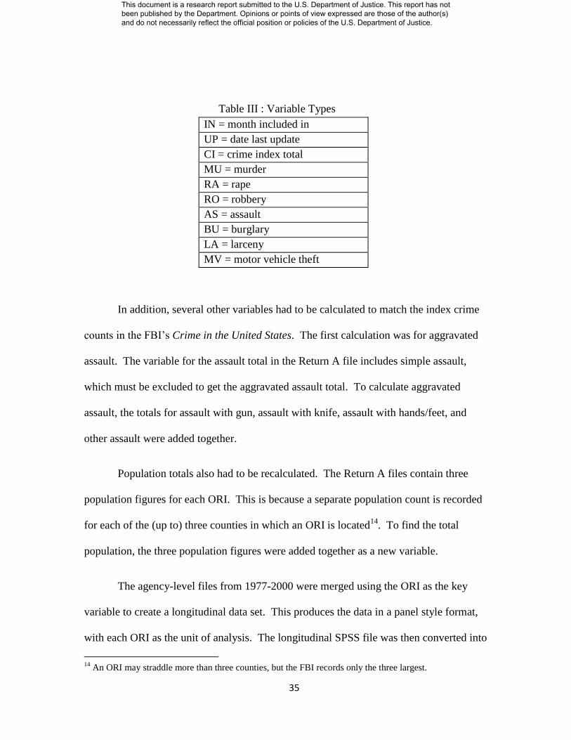
35

Table III : Variable Types

IN = month included in

UP = date last update

CI = crime index total

MU = murder

RA = rape

RO = robbery

AS = assault

BU = burglary

LA = larceny

MV = motor vehicle theft

In addition, several other variables had to be calculated to match the index crime

counts in the FBI’s Crime in the United States. The first calculation was for aggravated

assault. The variable for the assault total in the Return A file includes simple assault,

which must be excluded to get the aggravated assault total. To calculate aggravated

assault, the totals for assault with gun, assault with knife, assault with hands/feet, and

other assault were added together.

Population totals also had to be recalculated. The Return A files contain three

population figures for each ORI. This is because a separate population count is recorded

for each of the (up to) three counties in which an ORI is located14

. To find the total

population, the three population figures were added together as a new variable.

The agency-level files from 1977-2000 were merged using the ORI as the key

variable to create a longitudinal data set. This produces the data in a panel style format,

with each ORI as the unit of analysis. The longitudinal SPSS file was then converted into

14

An ORI may straddle more than three counties, but the FBI records only the three largest.


36

50 Microsoft Excel workbooks, one for each state. Each state workbook contained a total

of 18 worksheets. The first worksheet contained the identified reporting errors and a plot

of monthly crime data for each ORI. The second sheet contained the descriptive

information about an ORI including name, population count, data updated (for

identifying missing months), county, SMSA code, FBI population group, “covered by”

status15

, and reporting history. The remaining 16 worksheets contained the crime data for

each ORI. The monthly index crime required two worksheets, since Excel 2003 can only

hold 256 columns and each ORI contains 288 monthly crime data points (24 years x 12

months =288). This also includes two additional worksheets for the month-by-month

sum of the index crimes.

Exporting the data into Excel was done to facilitate the charting of data and to

allow for programming the imputation algorithms in Visual Basic for Applications

(VBA), which are included in Appendix C. As described above, a worksheet was created

to graph the ORI level crime data. This was done using a VBA macro to pull the

monthly index crime totals for the entire 1977-2000 time period. This allowed the

inspection of each of the over 17,000 ORIs individually. While this process was time-

consuming, it allowed for the human eye to detect anomalies that may go uncovered by

an algorithm. In addition, this process uncovered several patterns and types of missing

data that might have gone undetected.

15

This is explained in Section 3 below.


37

C. Graphical Data Analysis

The primary analysis tool for this project was the use of graphical methods to

analyze the UCR Offenses-Known data. Early adopters of this method have applied it to

a range of data types (Tufte 1983; Tufte 1990; Cleveland 1993; Cleveland 1994; Tufte

1997). Graphical analysis have also been used by criminologists to analyze homicide

data (Maltz 1998; Shon and Targonski 2003) and are a significant part of crime mapping

research and application.

Most researchers use graphs as means to display data, but graphs can also offer

insights and serve as an analytic tool (Maltz 1998). They become more applicable as

datasets become larger and standard statistical tests designed for samples become more

limited in their usefulness (Maltz 1998, 2009). UCR data are no exception, since it is

already quite large and will only expand with agencies converting to NIBRS.

The first step for this project will be to use graphical analysis for the data cleaning

and outlier detection. They will also be used to report the results of the data cleaning and

provide examples of data anomalies that were detected. Graphical analysis will also be

incorporated into the simulation results and to show the trends in missing data over time

by FBI group and state.

D. Data Cleaning

Despite the efforts of the FBI’s quality control mechanisms16

, data anomalies and

errors were found in the UCR files that had to be addressed before any imputation

16

For a detailed description of the FBI’s quality control mechanisms, see User Technology Associates

(1999) and Akiyama and Propheter (2005).


38

analysis was conducted. The following subsections detail the types of the anomalies and

outliers that were detected.

1. Agency Name Checks

After the files were merged, the first data-cleaning task performed was to check the

sequence of agency names over the 24-year period. This was done to ensure the ORI

code for each year refers to one and only one agency and to determine the years in which

the ORI existed.

2. True Missing

There is no stated flag code in the Return A file indicating if an ORI had

submitted valid data for a given month. However, after consulting with FBI staff, it was

determined that it was possible to identify if an agency had submitted data for a particular

month. Each month a Return A file is submitted to the FBI, the date the form was

received is recorded in the DATE LAST UPDATE field. If no Return A file was

received, the value is left blank. The Return A variable DATE LAST UPDATE can then

serve as a proxy for whether or not that month’s crime data are missing. Any month

with a missing value for DATE LAST UPDATE was recoded as a “true missing” value,

with a code of –99.

Without the DATE LAST UPDATE variable, it would not be possible to

distinguish a zero value as meaning “no crime” or “no report submitted.” As was

observed during the data cleaning, this is not a perfect indicator and there are many

exceptions. The following examples describe these exceptions and how they were

recoded.


39

3. Aggregation of Months

While crime data are supposed to be submitted on a monthly basis, not all

agencies adhere to this policy. The most common exceptions are reporting crime on a

quarterly, semiannual, or annual basis. Birmingham, AL (Figure 3) provides a good

example, because it used all three in reporting data between 1990 and 2000:

Figure 3. Quarterly, Semiannual and Annual Reporting Example

In addition, from 1994 to 1996 Birmingham reported data for all months, but the

annual total was distributed (approximately) equally to all months.

Aggregate reporting complicates accurately coding missing months, since the

system is set up for monthly reporting. For example, an annual reporter will report zero

index crimes for January through November and then have a high crime count in

December.

0

5,000

10,000

15,000

20,000

25,000

Jan

uar

y-7

7

Jan

uar

y-7

8

Jan

uar

y-7

9

Jan

uar

y-8

0

Jan

uar

y-8

1

Jan

uar

y-8

2

Jan

uar

y-8

3

Jan

uar

y-8

4

Jan

uar

y-8

5

Jan

uar

y-8

6

Jan

uar

y-8

7

Jan

uar

y-8

8

Jan

uar

y-8

9

Jan

uar

y-9

0

Jan

uar

y-9

1

Jan

uar

y-9

2

Jan

uar

y-9

3

Jan

uar

y-9

4

Jan

uar

y-9

5

Jan

uar

y-9

6

Jan

uar

y-9

7

Jan

uar

y-9

8

Jan

uar

y-9

9

Jan

uar

y-0

0

Nu

mb

er

of

Ind

ex

Cri

me

s

Quarterly, Semiannual and Annual Reporting: Birmingham, AL

Quarterly

Semiannual

Annual


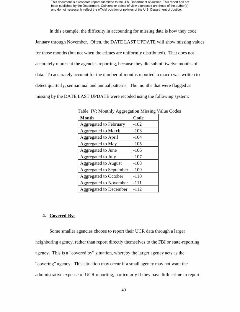
40

In this example, the difficulty in accounting for missing data is how they code

January through November. Often, the DATE LAST UPDATE will show missing values

for those months (but not when the crimes are uniformly distributed). That does not

accurately represent the agencies reporting, because they did submit twelve months of

data. To accurately account for the number of months reported, a macro was written to

detect quarterly, semiannual and annual patterns. The months that were flagged as

missing by the DATE LAST UPDATE were recoded using the following system:

Table IV: Monthly Aggregation Missing Value Codes

Month Code

Aggregated to February -102

Aggregated to March -103

Aggregated to April -104

Aggregated to May -105

Aggregated to June -106

Aggregated to July -107

Aggregated to August -108

Aggregated to September -109

Aggregated to October -110

Aggregated to November -111

Aggregated to December -112

4. Covered-Bys

Some smaller agencies choose to report their UCR data through a larger

neighboring agency, rather than report directly themselves to the FBI or state-reporting

agency. This is a “covered by” situation, whereby the larger agency acts as the

“covering” agency. This situation may occur if a small agency may not want the

administrative expense of UCR reporting, particularly if they have little crime to report.


41

If a small agency is covered by another agency, then its crime data are reported though

the larger agency. Often, the smaller agency will submit a report, but report no crime at

all, as its crime is aggregated into the covering agency. If an agency is “covered by”

another agency, then its data should not be considered missing.

The DATE LAST UPDATE may also indicate non-reporting for the covered-by

agency. For the analysis of missing data, the “covering” agency’s missing data status is

used and not the “covered-by” (smaller) agency. The missing value code of -85 was

assigned to months in which the agency was covered by another agency.

There was an issue with raw data files in 1980 and 1995, where the covered-by

variables were not in the raw ICPSR data file. To address this gap, some assumptions

were made to fill in the missing years. If an agency was covered by the same “covering”

agency in the years surrounding the missing year (1979 and 1981 for 1980; 1994 and

1996 for 1995), and the agency had no crime in the missing year, then it was assumed the

same agency was covering in the missing year. This took care of virtually every case of

missing covered-by data.

5. Non-Existent Agencies

Not every ORI existed every year between 1977 and 2000. For the years an ORI

was not in existence, a new code was needed to account for this status. Otherwise, it

would have been considered a missing value and would overstate the missing data. An

imputation algorithm might also try to impute for values in which an agency did not exist.

The missing value code of -80 was assigned to months in which the agency did not exist.


42

6. Rule of 20

As described earlier, the main method to determine a true missing data point was

based on the DATE LAST UPDATE variable. There were some cases where an ORI

submitted a Return A report for that month, but the crime count was zero. For many

small agencies with low crime, it is possible to not have any index crimes for a month.

However, there were instances of ORIs that consistently reported many index crimes, the

DATE LAST UPDATE indicated a Return A form was submitted, but the index crime

for the month was zero. Figure 4 illustrates an example for the Bay State MI Police. The

red circle shows a gap where no index crimes were reported. However, during those

months the Bay State MI Police were reporting 12 months of crime data per year

according to the DATE LAST UPDATE variable.

Figure 4. Rule of 20

0

20

40

60

80

100

120

140

160

180

200

Jan

uar

y-7

7

Jan

uar

y-7

8

Jan

uar

y-7

9

Jan

uar

y-8

0

Jan

uar

y-8

1

Jan

uar

y-8

2

Jan

uar

y-8

3

Jan

uar

y-8

4

Jan

uar

y-8

5

Jan

uar

y-8

6

Jan

uar

y-8

7

Jan

uar

y-8

8

Jan

uar

y-8

9

Jan

uar

y-9

0

Jan

uar

y-9

1

Jan

uar

y-9

2

Jan

uar

y-9

3

Jan

uar

y-9

4

Jan

uar

y-9

5

Jan

uar

y-9

6

Jan

uar

y-9

7

Jan

uar

y-9

8

Jan

uar

y-9

9

Jan

uar

y-0

0

Nu

mb

er

of

Ind

ex

Cri

me

s

Rule of 20: Bay State Police, MI


43

To account for such ORIs, a rule was established that an ORI with an average of

20 or more index crimes per month could not have zero index crimes in a month, if the

DATE LAST UPDATE flagged the Return A as being submitted. These instances were

coded as missing with a value of -90.17

7. Negative Values

During the data screening, a number of negative values for index crime counts

were discovered. The FBI does allow for adjustments for instances where in from prior

months crimes had been over-reported, such as cases that were later determined to be

false (unfounded) reports, or for reclassification (FBI 1984).

However, some of the negative values were obviously out of range and are most

likely data entry errors. In the entire dataset, 5081 negative values were found. Only 142

were lower than -3 and were reassigned to be missing values (-99). The cutoff for

determining what was a “true” negative number and a “real” negative number could not

be done with exact precision. However, the cutoff of -3 was based on logical grounds of

reporting and average crime counts. In order to have 4 unfounded crimes, it would likely

have to have an average of at least 10 crimes a month, which is a very conservative

estimate. To arrive at monthly value of -4, it would require, for example, 2 actual crimes

and 6 unfounded, which would be a very unlikely occurrence.

17

In addition to these cases, there were some instances of agencies with average crime counts that were less

than 20 showing zero crime and a date for the DATE LAST UPDATE. These were, in the researcher’s

judgment, data points that were missing.


44

Figure 5. Negative Crime Values, 1977-2000

For the purpose of screening outliers, -4 was determined as the cutoff for

legitimate values. Any values less than –4 were recoded as missing values (-99), since

they were most likely data entry errors.

8. Outlier Values

As part of the data screening process, each ORIs trend was examined graphically.

In the process, outliers were detected for the crime index. To prevent these values from

skewing the imputation results, the outlier values were recoded as –90. In a separate

Excel sheet, the old values were retained if they needed to be accessed.

A subtype of outlier values were the “999,” “9999,” and “99999” crime counts.

Below in figure 6 is an example from Durango, CO:

0

10

20

30

40

50

60

70

80

-20 -19 -18 -17 -16 -15 -14 -13 -12 -11 -10 -9 -8 -7 -6 -5 -4 -3

Fre

qu

en

cy o

f N

eg

ati

ve C

rim

e V

alu

es

Negative Crime Values, 1977-2000


45

Figure 6. Outlier 9999 Value for Crime Index, Durango, CO

In September 1993, Durango reported 9999 assault cases, which pushed the crime

index to 10,002. This was an obvious outlier value and would have caused many

problems when trying to impute for Durango including such a value in the crime index.

In situations where a single crime was responsible causing the missing crime index, a

separate code was created for each crime, -9x for the x-th index crime missing. Thus, the

totality of all codes used for individual crimes are as follows:

0

2,000

4,000

6,000

8,000

10,000

12,000Ja

nu

ary-

77

Jan

uar

y-7

8

Jan

uar

y-7

9

Jan

uar

y-8

0

Jan

uar

y-8

1

Jan

uar

y-8

2

Jan

uar

y-8

3

Jan

uar

y-8

4

Jan

uar

y-8

5

Jan

uar

y-8

6

Jan

uar

y-8

7

Jan

uar

y-8

8

Jan

uar

y-8

9

Jan

uar

y-9

0

Jan

uar

y-9

1

Jan

uar

y-9

2

Jan

uar

y-9

3

Jan

uar

y-9

4

Jan

uar

y-9

5

Jan

uar

y-9

6

Jan

uar

y-9

7

Jan

uar

y-9

8

Jan

uar

y-9

9

Jan

uar

y-0

0

Outlier 9999 Value for Crime IndexDurango, CO


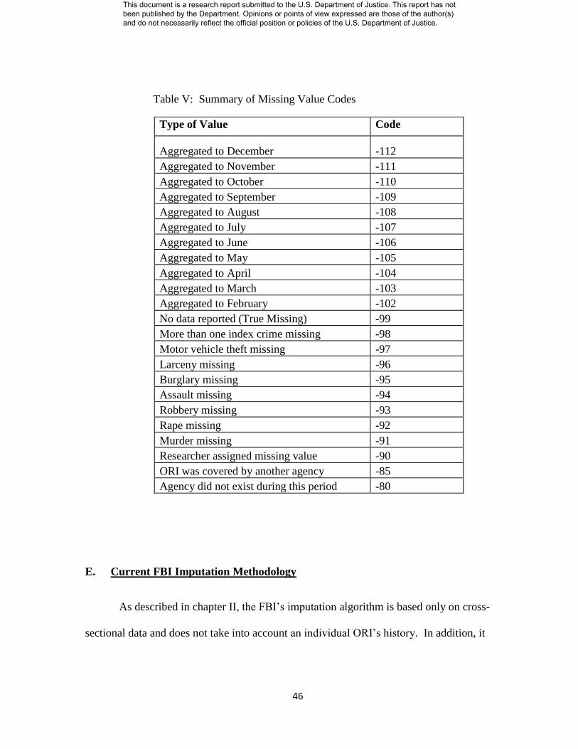
46

Table V: Summary of Missing Value Codes

Type of Value Code

Aggregated to December -112

Aggregated to November -111

Aggregated to October -110

Aggregated to September -109

Aggregated to August -108

Aggregated to July -107

Aggregated to June -106

Aggregated to May -105

Aggregated to April -104

Aggregated to March -103

Aggregated to February -102

No data reported (True Missing) -99

More than one index crime missing -98

Motor vehicle theft missing -97

Larceny missing -96

Burglary missing -95

Assault missing -94

Robbery missing -93

Rape missing -92

Murder missing -91

Researcher assigned missing value -90

ORI was covered by another agency -85

Agency did not exist during this period -80

E. Current FBI Imputation Methodology

As described in chapter II, the FBI’s imputation algorithm is based only on cross-

sectional data and does not take into account an individual ORI’s history. In addition, it


47

assumes that similar agencies will have comparable crime rates. This does not take into

account agency level or geographic differences.

F. Longitudinal Imputation Method

As an alternative, a longitudinal method was explored for imputing an agency’s

crime data. This takes into account an agency’s past reporting behavior, account for

seasonality, and allows for crime estimates at more granular levels, such as ORI and

county levels. For agencies reporting less than 3 months of data, the imputation

algorithm will take the group crime rate for that ORI in the current year divided by the

group rate in the prior year, to arrive at the change estimate. This change estimate is then

multiplied by the data reported in the prior year.

As with the FBI method, the group consists of those agencies in the same state

and same population range that provide crime reports for the full 12 months. However,

this method uses the group rates for the change estimate, rather than for the index crime

level estimate.

For an agency reporting 3-11 months of data, the longitudinal imputation formula

is based on that agency’s year-to-year increase for the months reported. That is, it

assumes that the agency has the same seasonal trajectory in both years, so it multiplies

the agency’s missing months’ data with the percent change factor from the FBI group.

If {X}t is the set of months for which agency A reported crime in year t and {Y}t

is the set of months for which it did not report crime. Then


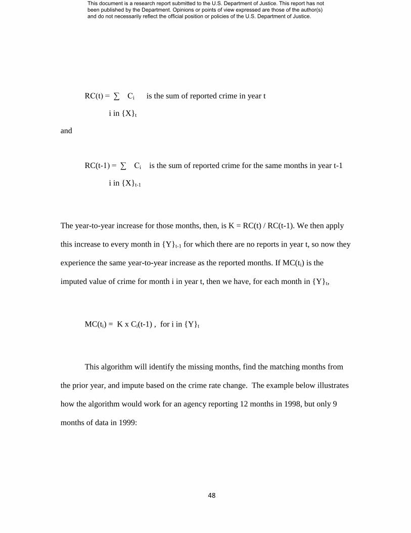
48

RC(t) = ∑ Ci is the sum of reported crime in year t

i in {X}t

and

RC(t-1) = ∑ Ci is the sum of reported crime for the same months in year t-1

i in {X}t-1

The year-to-year increase for those months, then, is K = RC(t) / RC(t-1). We then apply

this increase to every month in {Y}t-1 for which there are no reports in year t, so now they

experience the same year-to-year increase as the reported months. If MC(ti) is the

imputed value of crime for month i in year t, then we have, for each month in {Y}t,

MC(ti) = K x Ci(t-1) , for i in {Y}t

This algorithm will identify the missing months, find the matching months from

the prior year, and impute based on the crime rate change. The example below illustrates

how the algorithm would work for an agency reporting 12 months in 1998, but only 9

months of data in 1999:


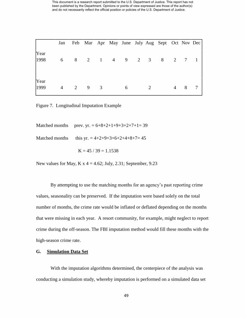
49

Jan Feb Mar Apr May June July Aug Sept Oct Nov Dec

Year

1998 6 8 2 1 4 9 2 3 8 2 7 1

Year

1999 4 2 9 3 6 2 4 8 7

Figure 7. Longitudinal Imputation Example

Matched months prev. yr. = 6+8+2+1+9+3+2+7+1= 39

Matched months this yr. = 4+2+9+3+6+2+4+8+7= 45

K = 45 / 39 = 1.1538

New values for May, K x 4 = 4.62; July, 2.31; September, 9.23

By attempting to use the matching months for an agency’s past reporting crime

values, seasonality can be preserved. If the imputation were based solely on the total

number of months, the crime rate would be inflated or deflated depending on the months

that were missing in each year. A resort community, for example, might neglect to report

crime during the off-season. The FBI imputation method would fill these months with the

high-season crime rate.

G. Simulation Data Set

With the imputation algorithms determined, the centerpiece of the analysis was

conducting a simulation study, whereby imputation is performed on a simulated data set


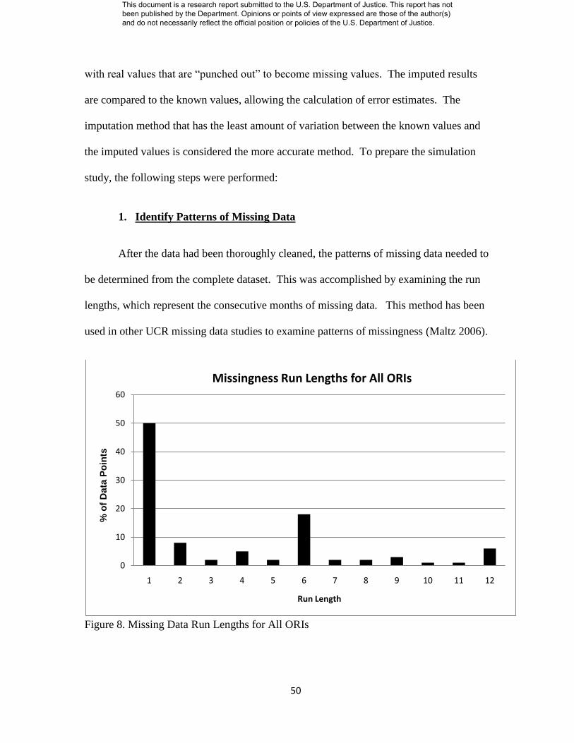
50

with real values that are “punched out” to become missing values. The imputed results

are compared to the known values, allowing the calculation of error estimates. The

imputation method that has the least amount of variation between the known values and

the imputed values is considered the more accurate method. To prepare the simulation

study, the following steps were performed:

1. Identify Patterns of Missing Data

After the data had been thoroughly cleaned, the patterns of missing data needed to

be determined from the complete dataset. This was accomplished by examining the run

lengths, which represent the consecutive months of missing data. This method has been

used in other UCR missing data studies to examine patterns of missingness (Maltz 2006).

Figure 8. Missing Data Run Lengths for All ORIs

0

10

20

30

40

50

60

1 2 3 4 5 6 7 8 9 10 11 12

% o

f D

ata

Po

ints

Run Length

Missingness Run Lengths for All ORIs


51

The results of the run length analysis reveal a skewed distribution of data points,

with 50% of the data missing for only one consecutive month. There is another increase

when we get to six months of consecutive months missing, which may be driven by

agencies reporting for half the year. Finally, 6% of the data points are missing run

lengths of 12 months, which represents the percentage of agencies that reported zero

months of data.

2. Identify Full Reporting Agencies

The next step was to identify all ORIs that had full reporting for years 1989 to

1999. The time frame was narrowed from the original dataset, to allow for more ORIs to

be included in the study. There were a total of 4,765 ORIs that met this criterion and

served as the basis for the simulation study sample. A breakdown of these ORIs by FBI

state and group can be found in figures 9 and 10. Note that Group I has the fewest such

ORIs, since there are very few ORIs in this group, which represents the most populous

cities.


52

Figure 9. Number of ORIs that Qualify for Imputation by State

0 100 200 300 400 500 600 700 800

DE

KS

NH

AK

HI

WI

IL

CO

ND

SD

ID

NV

NM

MS

GA

UT

RI

AZ

LA

WY

TN

PA

MA

OR

ME

WV

CT

MO

WA

MD

AR

OH

NC

IN

NB

VA

MN

NY

MI

OK

NJ

CA

TX

Number of ORIs that Qualify for Imputation by StateBased on Complete Reporting


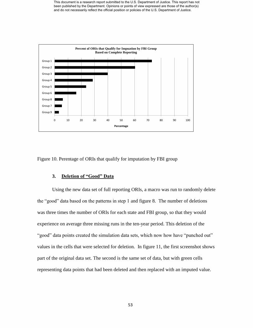
53

0 10 20 30 40 50 60 70 80 90 100

Group 9

Group 7

Group 8

Group 6

Group 5

Group 4

Group 3

Group 2

Group 1

Percentage

Percent of ORIs that Qualify for Impuation by FBI Group

Based on Complete Reporting

Figure 10. Perentage of ORIs that qualify for imputation by FBI group

3. Deletion of “Good” Data

Using the new data set of full reporting ORIs, a macro was run to randomly delete

the “good” data based on the patterns in step 1 and figure 8. The number of deletions

was three times the number of ORIs for each state and FBI group, so that they would

experience on average three missing runs in the ten-year period. This deletion of the

“good” data points created the simulation data sets, which now how have “punched out”

values in the cells that were selected for deletion. In figure 11, the first screenshot shows

part of the original data set. The second is the same set of data, but with green cells

representing data points that had been deleted and then replaced with an imputed value.


54

Figure 11. Screenshots of Simulated Data


55

The leftmost column is the ORI code and the rest of the columns represent the monthly

crime data. The variables in the first column are for each month, with “CI” standing for

“Crime Index,” followed by the two-digit year and then two-digit month.

There were a total of 60 test files created, one for all the ORIs, one for each of the

nine FBI groups, and one for each state. This was done to permit comparisons by FBI

group and state.

4. Running Imputations

Each imputation method was run and the imputed values were compared to the

actual values. Comparisons were based on the absolute difference and root mean square

difference. The analysis based on the yearly crime totals, as well as the aggregate of all

the years. The Visual Basic code used in the Excel analysis can be found in Appendix C.


56

IV. RESULTS

A. Introduction

After the data are cleaned, the next step is to analyze the patterns and levels of

missing data. This was performed by using the new missing value codes that were

applied during the data cleaning. Missing data was disaggregated and analyzed by the

total United States, FBI group, and state. The simulation data sets are then run and also

analyzed by total United States, FBI Group, and run length.

B. Descriptive Statistics of Missing Data

1. New Definition of Missingness

As part of the yearly CIUS, the FBI publishes the population coverage of the

UCR. However, for an agency to be considered “covered” for its population, the FBI

only requires that it submit one month of data. In a case where an agency only submits

one month, the FBI would have to impute for the remaining 11 months of data. This can

result in an underestimate of the missing data.

For this study, the amount of missing data is based on the new missing value codes.

Therefore, it accounts for all the data issues described in Chapter III including outlier

values, covered-by agencies, aggregated reporting, and incorrect negative values.


57

2. Missing Data for the Total United States

Figure 12. Percent of Missing Data All ORIs, 1977-2000

Between 1977 and 1987, the level of missing data held fairly consistent around

15% for the raw count and 5% of the population. In 1988, there is a spike at the national

level, which was the result of state-level problems with Florida and Kentucky. Both

states reported 100% missing data for that year, due to data quality issues (FBI 2007).

The number of missing data then began to increase through the late 1990s, with a slight

decrease in 2000.

3. Missing Data by Group

While missingness at the total US level provides insight to overall trends, it is

necessary to disaggregate to lower level geographies to get a better understanding of

0%

10%

20%

30%

40%

50%

60%

70%

80%

90%

100%

19

77

19

78

19

79

19

80

19

81

19

82

19

83

19

84

19

85

19

86

19

87

19

88

19

89

19

90

19

91

19

92

19

93

19

94

19

95

19

96

19

97

19

98

19

99

20

00

Percent of Missing Data All ORIs1977-2000

Weighted by population Unweighted


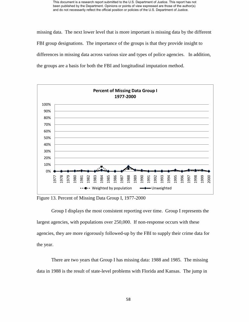
58

missing data. The next lower level that is more important is missing data by the different

FBI group designations. The importance of the groups is that they provide insight to

differences in missing data across various size and types of police agencies. In addition,

the groups are a basis for both the FBI and longitudinal imputation method.

Figure 13. Percent of Missing Data Group I, 1977-2000

Group I displays the most consistent reporting over time. Group I represents the

largest agencies, with populations over 250,000. If non-response occurs with these

agencies, they are more rigorously followed-up by the FBI to supply their crime data for

the year.

There are two years that Group I has missing data: 1988 and 1985. The missing

data in 1988 is the result of state-level problems with Florida and Kansas. The jump in

0%

10%

20%

30%

40%

50%

60%

70%

80%

90%

100%

19

77

19

78

19

79

19

80

19

81

19

82

19

83

19

84

19

85

19

86

19

87

19

88

19

89

19

90

19

91

19

92

19

93

19

94

19

95

19

96

19

97

19

98

19

99

20

00

Percent of Missing Data Group I1977-2000



59

missing data for 1984 was the result of the Chicago Police not reporting 12 months of

data.

Figure 14. Percent of Missing Data Group II, 1977-2000

0%

10%

20%

30%

40%

50%

60%

70%

80%

90%

100%

19

77

19

78

19

79

19

80

19

81

19

82

19

83

19

84

19

85

19

86

19

87

19

88

19

89

19

90

19

91

19

92

19

93

19

94

19

95

19

96

19

97

19

98

19

99

20

00

Percent of Missing Data Group II1977-2000



60

Figure 15. Percent of Missing Data Group III, 1977-2000

Figure 16. Percent of Missing Data Group IV, 1977-2000

0%

10%

20%

30%

40%

50%

60%

70%

80%

90%

100%

19

77

19

78

19

79

19

80

19

81

19

82

19

83

19

84

19

85

19

86

19

87

19

88

19

89

19

90

19

91

19

92

19

93

19

94

19

95

19

96

19

97

19

98

19

99

20

00

Percent of Missing Data Group III1977-2000


0%

10%

20%

30%

40%

50%

60%

70%

80%

90%

100%

19

77

19

78

19

79

19

80

19

81

19

82

19

83

19

84

19

85

19

86

19

87

19

88

19

89

19

90

19

91

19

92

19

93

19

94

19

95

19

96

19

97

19

98

19

99

20

00

Percent of Missing Data Group IV1977-2000



61

Figure 17. Percent of Missing Data Group V, 1977-2000

Figure 18. Percent of Missing Data Group VI, 1977-2000

0%

10%

20%

30%

40%

50%

60%

70%

80%

90%

100%

19

77

19

78

19

79

19

80

19

81

19

82

19

83

19

84

19

85

19

86

19

87

19

88

19

89

19

90

19

91

19

92

19

93

19

94

19

95

19

96

19

97

19

98

19

99

20

00

Percent of Missing Data Group V1977-2000


0%

10%

20%

30%

40%

50%

60%

70%

80%

90%

100%

19

77

19

78

19

79

19

80

19

81

19

82

19

83

19

84

19

85

19

86

19

87

19

88

19

89

19

90

19

91

19

92

19

93

19

94

19

95

19

96

19

97

19

98

19

99

20

00

Percent of Missing Data Group VI1977-2000



62

Figure 19. Percent of Missing Data Group VII, 1977-2000

Groups II through VII all show a similar pattern, with small amounts of missing data

between 1977 and 1992. The level of missing data becomes slightly higher as the group

numbers get larger, with the population of the agencies becoming smaller. From 1993

through 2000, there is an overall upward trend in missing data across groups.

0%

10%

20%

30%

40%

50%

60%

70%

80%

90%

100%

19

77

19

78

19

79

19

80

19

81

19

82

19

83

19

84

19

85

19

86

19

87

19

88

19

89

19

90

19

91

19

92

19

93

19

94

19

95

19

96

19

97

19

98

19

99

20

00

Percent of Missing Data Group VII1977-2000



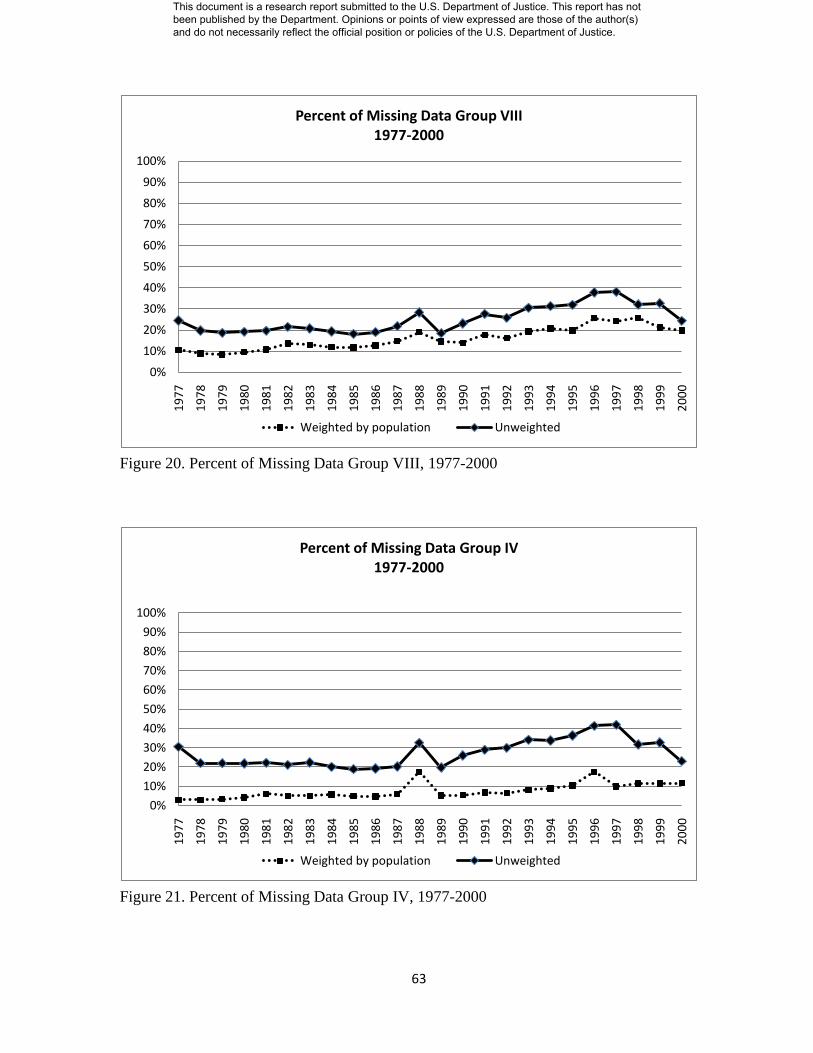
63

Figure 20. Percent of Missing Data Group VIII, 1977-2000

Figure 21. Percent of Missing Data Group IV, 1977-2000

0%

10%

20%

30%

40%

50%

60%

70%

80%

90%

100%

19

77

19

78

19

79

19

80

19

81

19

82

19

83

19

84

19

85

19

86

19

87

19

88

19

89

19

90

19

91

19

92

19

93

19

94

19

95

19

96

19

97

19

98

19

99

20

00

Percent of Missing Data Group VIII1977-2000


0%

10%

20%

30%

40%

50%

60%

70%

80%

90%

100%

19

77

19

78

19

79

19

80

19

81

19

82

19

83

19

84

19

85

19

86

19

87

19

88

19

89

19

90

19

91

19

92

19

93

19

94

19

95

19

96

19

97

19

98

19

99

20

00

Percent of Missing Data Group IV1977-2000



64

Group IV, which represents Suburban Counties, including State Police with no

population, saw the highest level of unweighted missing data of all the groups. When

weighted by population, the missing data level drops, since the agencies are some of the

smallest in terms of population coverage. For charts of the missing data for all 50 states,

please see Appendix D.

4. Frequency of Missing Value Codes

The complete dataset for 1977-2000 contains a total of 5,779,295 cells. 62.5%

represent valid data points with crime values, including true zero values. 943,982

(16.3%) were identified as missing values using the “DATE LAST UPDATE” variable

on the raw Return A file. In between is a combination of aggregated reporting, non-

existent ORIs, missing values we assigned, and individual missing crimes. Identifying

the missing values monthly Return A form using the “DATE LAST UPDATE” variable

is an all or nothing proposition. If the month had a date and was considered a valid

reporting month, there is no special FBI code to indicate missing values on the individual

crimes. Therefore, any missing values for the individual crimes were identified by the

researcher. That makes a total of 11,241 (0.19%) of the total data points that were

deemed to be missing even though they had a data reported for the “Date Updated”

variable. While this is a very small percentage, the scale to which the values were

outside the norm could severely skew an imputation algorithm or other statistical

analysis. For example, some agencies reported values such as “99999.” These likely

represent a code for a missing value, but treating them as a valid data point could

severely skew statistical results.


65

Table VI: Frequency of Missing Value Codes, All ORIs, 1977-2000

Type of Value Code Number of Data

Points

% of Total

Aggregated to December -112 76,222 1.3%

Aggregated to November -111 91 0.0%

Aggregated to October -110 23 0.0%

Aggregated to September -109 271 0.0%

Aggregated to August -108 84 0.0%

Aggregated to July -107 18 0.0%

Aggregated to June -106 545 0.0%

Aggregated to May -105 27 0.0%

Aggregated to April -104 4 0.0%

Aggregated to March -103 219 0.0%

Aggregated to February -102 3 0.0%

No data reported (True Missing) -99 943,982 16.3%

More than one index crime missing -98 9,825 0.2%

Motor vehicle theft missing -97 56 0.0%

Larceny missing -96 79 0.0%

Burglary missing -95 59 0.0%

Assault missing -94 103 0.0%

Robbery missing -93 48 0.0%

Rape missing -92 144 0.0%

Murder missing -91 1 0.0%

Researcher assigned missing value -90 926 0.0%

ORI was covered by another agency -85 421,500 7.3%

Agency did not exist during this period -80 712,056 12.3%

Negative Value -1 131 0.0%




Non-Missing Value Reported Value 3,612,862 62.5%


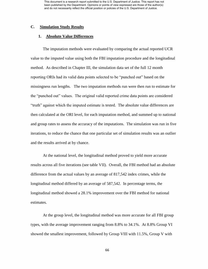
66

C. Simulation Study Results

1. Absolute Value Differences

The imputation methods were evaluated by comparing the actual reported UCR

value to the imputed value using both the FBI imputation procedure and the longitudinal

method. As described in Chapter III, the simulation data set of the full 12 month

reporting ORIs had its valid data points selected to be “punched out” based on the

missingness run lengths. The two imputation methods run were then run to estimate for

the “punched out” values. The original valid reported crime data points are considered

“truth” against which the imputed estimate is tested. The absolute value differences are

then calculated at the ORI level, for each imputation method, and summed up to national

and group rates to assess the accuracy of the imputations. The simulation was run in five

iterations, to reduce the chance that one particular set of simulation results was an outlier

and the results arrived at by chance.

At the national level, the longitudinal method proved to yield more accurate

results across all five iterations (see table VII). Overall, the FBI method had an absolute

difference from the actual values by an average of 817,542 index crimes, while the

longitudinal method differed by an average of 587,542. In percentage terms, the

longitudinal method showed a 28.1% improvement over the FBI method for national

estimates.

At the group level, the longitudinal method was more accurate for all FBI group

types, with the average improvement ranging from 8.8% to 34.1%. At 8.8% Group VI

showed the smallest improvement, followed by Group VIII with 11.5%, Group V with


67

21.7%, Group IV at 27.4%, Group III at 28.3%, Group II at 30.0%, Group IV at 30.3%,

Group VII at 33.1% and Group I at 34.1%.


68

Table VII: Simulation Results of Absolute Differences

Iteration 1 Iteration 2 Iteration 3 Iteration 4 Iteration 5

FBI Method

LNG Method FBI Method

LNG Method

FBI Method



LNG Method Average Improvement Across Simulations

Total US 877,447 640,570 807,403 607,861 809,683 556,381 786,880 571,468 806,296 561,431 28.1%

Group I 146,798 99,103 179,280 128,210 209,584 121,665 155,259 94,289 173,078 125,951 34.1%

Group II 82,062 69,651 112,177 65,914 82,702 62,512 94,072 68,088 119,626 77,089 30.0%

Group III 95,953 60,413 88,506 64,232 80,978 64,172 88,645 61,396 81,962 62,737 28.2%

Group IV 77,379 57,783 88,059 58,341 87,420 64,211 88,644 67,751 86,453 62,446 27.4%

Group V 84,256 66,397 93,762 69,792 75,462 61,418 82,434 68,792 83,193 61,575 21.7%

Group VI 60,112 55,190 64,884 56,748 62,070 57,435 59,695 55,197 61,479 56,569 8.8%

Group VII 31,148 21,558 30,229 20,706 31,950 23,334 35,560 21,676 34,239 21,925 33.1%

Group VIII 41,720 37,591 48,246 40,534 42,808 39,463 44,287 38,945 42,398 37,717 11.5%

Group IV 126,180 96,705 123,489 85,984 124,847 76,471 113,856 81,931 124,587 85,900 30.3%


69

In addition to measuring the absolute value accuracy by FBI group number, the

same analysis was conducted by the missing data run length. This allows a different drill

down of the analysis, to see how the accuracy varied by amount of missing data the

method was imputing for in the simulation data set (see tables VIII and IX below).

Table VIII: Simulation Results of Average Absolute Value Differences by Run Length

Average Across the Five Iterations

Run Length

FBI Imputation Method

Longitudinal Imputation Method

% Improvement with the Longitudinal

1 101,299 111,905 -10.5%

2 31,473 32,426 -3.0%

3 9,615 9,589 0.3%

4 30,372 27,540 9.3%

5 15,672 18,759 -19.7%

6 183,165 174,142 4.9%

7 22,813 23,507 -3.0%

8 28,051 25,664 8.5%

9 49,411 57,422 -16.2%

10 34,928 11,768 66.3%

11 35,500 11,621 67.3%

12 275,242 83,200 69.8%

Total 817,542 587,542 28.1%


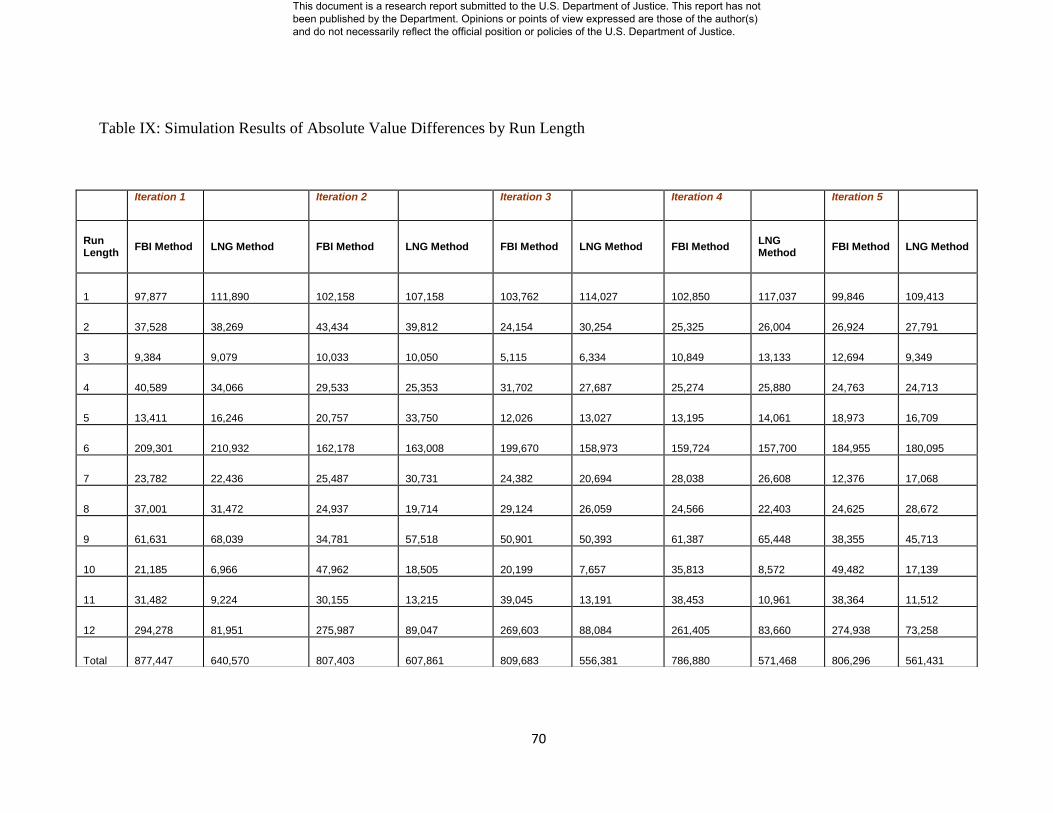
70

Table IX: Simulation Results of Absolute Value Differences by Run Length

Iteration 1 Iteration 2 Iteration 3 Iteration 4 Iteration 5

Run Length

FBI Method LNG Method FBI Method LNG Method FBI Method LNG Method FBI Method LNG Method

FBI Method LNG Method

1 97,877 111,890 102,158 107,158 103,762 114,027 102,850 117,037 99,846 109,413

2 37,528 38,269 43,434 39,812 24,154 30,254 25,325 26,004 26,924 27,791

3 9,384 9,079 10,033 10,050 5,115 6,334 10,849 13,133 12,694 9,349

4 40,589 34,066 29,533 25,353 31,702 27,687 25,274 25,880 24,763 24,713

5 13,411 16,246 20,757 33,750 12,026 13,027 13,195 14,061 18,973 16,709

6 209,301 210,932 162,178 163,008 199,670 158,973 159,724 157,700 184,955 180,095

7 23,782 22,436 25,487 30,731 24,382 20,694 28,038 26,608 12,376 17,068

8 37,001 31,472 24,937 19,714 29,124 26,059 24,566 22,403 24,625 28,672

9 61,631 68,039 34,781 57,518 50,901 50,393 61,387 65,448 38,355 45,713

10 21,185 6,966 47,962 18,505 20,199 7,657 35,813 8,572 49,482 17,139

11 31,482 9,224 30,155 13,215 39,045 13,191 38,453 10,961 38,364 11,512

12 294,278 81,951 275,987 89,047 269,603 88,084 261,405 83,660 274,938 73,258

Total 877,447 640,570 807,403 607,861 809,683 556,381 786,880 571,468 806,296 561,431


71

While the overall improvement with the longitudinal method was 28.1% versus

the FBI method, the results varied depending on the missing run length. The longer run

lengths of 10, 11, and 12 months showed significant improvement with the longitudinal

method. This should be expected, since the FBI imputation for these run lengths is not

based on the agency’s own data, but on “similar” agencies (12-month reporters in the

same state and population group).

The 10-month run length improved by 66.3%, 11 months by 67.3%, and 12

months by 69.8%. For the remaining run lengths, the results were varied. Some showed

moderate improvement, such as run length 4 (9.3%), run length 6 (4.9%), and run length

8 (8.5%). Run length 3 showed only marginal improvement with 0.3% improvement.

For run lengths 1, 2, 5, 7, and 9, the FBI method proved to be more accurate. For these

the improvement with the longitudinal method was -10.5% (run length 1), -3.0% (run

length 2), -19.7% (run length 5), -3.0% (run length 7), and -16.2% (run length 9).

2. Crime Index Level Accuracy

The absolute value differences provide a view of how accurate each method is

against the actual values, but it does not show the impact to overall crime level estimates.

To do this, the crime totals of the simulation data set were summed for all years. From

1989-1999, the 4,765 full reporting ORIs in the simulation data set had 90,025,341 total

index crimes. Across the five iterations, the FBI method estimates ranged from

89,799,028 to 89,913,536 for an average of 89,857,809. The longitudinal method

estimates ranged from 89,999,605 to 90,049,393 for an average of 90,026,838 (see table

X).


72

Table X: Comparison of Crime Count Totals

Iteration 1 Iteration 2 Iteration 3 Iteration 4 Iteration 5 Average

Actual 90,025,341 90,025,341 90,025,341 90,025,341 90,025,341 90,025,341

FBI 89,834,855 89,894,019 89,799,028 89,913,536 89,847,604 89,857,809

Lng 90,049,393 90,035,895 90,030,660 89,999,605 90,018,638 90,026,838

Figure 22. Comparison of Crime Count Totals

Across all five iterations, the FBI method consistently underestimated the level of

crime compared to the actual. The greatest underestimation was in iteration 3 with

-0.25%, followed by iteration 1 with -0.21% (see table XI). The closest estimate for the

88,500,000

88,700,000

88,900,000

89,100,000

89,300,000

89,500,000

89,700,000

89,900,000

90,100,000

90,300,000


Comparison of Crime Count TotalsTotal US

Actual FBI Method Longitudinal Method


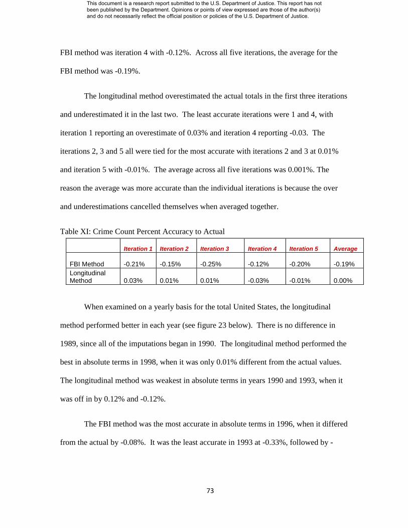
73

FBI method was iteration 4 with -0.12%. Across all five iterations, the average for the

FBI method was -0.19%.

The longitudinal method overestimated the actual totals in the first three iterations

and underestimated it in the last two. The least accurate iterations were 1 and 4, with

iteration 1 reporting an overestimate of 0.03% and iteration 4 reporting -0.03. The

iterations 2, 3 and 5 all were tied for the most accurate with iterations 2 and 3 at 0.01%

and iteration 5 with -0.01%. The average across all five iterations was 0.001%. The

reason the average was more accurate than the individual iterations is because the over

and underestimations cancelled themselves when averaged together.

Table XI: Crime Count Percent Accuracy to Actual


FBI Method -0.21% -0.15% -0.25% -0.12% -0.20% -0.19%

Longitudinal Method 0.03% 0.01% 0.01% -0.03% -0.01% 0.00%

When examined on a yearly basis for the total United States, the longitudinal

method performed better in each year (see figure 23 below). There is no difference in

1989, since all of the imputations began in 1990. The longitudinal method performed the

best in absolute terms in 1998, when it was only 0.01% different from the actual values.

The longitudinal method was weakest in absolute terms in years 1990 and 1993, when it

was off in by 0.12% and -0.12%.

The FBI method was the most accurate in absolute terms in 1996, when it differed

from the actual by -0.08%. It was the least accurate in 1993 at -0.33%, followed by -


74

0.29% in 1994, -0.27% in 1998, -0.26% in 1990, -0.23% in 1997 and 1999, -0.18% in

1991 and 1992, and -0.16% in 1995.

1989 1990 1991 1992 1993 1994 1995 1996 1997 1998 1999

FBI % Diff 0.00% -0.26% -0.18% -0.18% -0.33% -0.29% -0.16% -0.08% -0.23% -0.27% -0.23%

Longitudinal % Diff 0.00% 0.12% -0.08% 0.10% -0.12% -0.10% 0.02% 0.02% 0.09% 0.01% -0.04%

-0.40%

-0.30%

-0.20%

-0.10%

0.00%

0.10%

0.20%

0.30%

% D

iffe

re

nc

e fr

om

Ac

tua

l C

rim

e In

de

x

Figure 23. Yearly differences of imputation methods for Total US based on the average

of the five iterations


75

V. DISCUSSION AND CONCLUSION

A. Discussion

The purpose of this research was to 1) Clean the Offenses-Known UCR agency level files

and create a single longitudinal data set; 2) Analyze the type and extent of data errors to

determine patterns of missing data; and 3) Use a simulation data set of complete reporting ORIs

to determine the accuracy of the FBI cross-sectional imputation methodology against a

competing longitudinal method.

The missing data analysis found that there was an upward trend in the amount of missing

data in the UCR program beginning in the late 1980s through the ends of the 1990s. The growth

in missing data was not consistent among the different FBI population groups, with group I

showing consistent reporting over time and group II with only a slight increase in the 1990s. The

remaining groups III-IV, which constitute the smaller agencies, saw larger increases in missing

data over time. A similar pattern was present for the level of missing data, with groups I and II

having the strongest reporting, while groups III-IV reporting higher levels of missing data.

The data cleaning process revealed a number of unusual data artifacts, which required

recoding to properly analyze the missing data. Some of these artifacts were a known issue in

UCR data; others had not been documented and were ones not anticipated. The aggregation of

data into quarterly, semiannual and annual reporting had been a known issue that was quantified

as part of the analysis. However, what was more unusual were agencies that aggregated data

outside of those patterns. There were 250 data points (<.01% of the total) that reported

aggregated data in the months of February, April, May, July, August, October or November.

These don’t fit into the quarterly, semiannual, or annual reporting months patterns. It is possible


76

to see how this could happen for agencies that were reporting data late and might send two

months of data in a single monthly report.

Negative values are another known possibility in UCR data that can be legitimate values.

Police agencies can submit negative values as an accounting mechanism to adjust for unfounded

crimes. What was not expected was that some ORIs have reported negative values below -20.

While some negative values were to be expected, it seemed reasonable to set a cut off of -4 and

deem any value lower than that to be a missing value.

Outlier values were also present in the UCR crime index data. These typically were

either “999,” “9999,” or “99999.” The most likely explanation for these is that police agencies

were using these as their own missing value codes. However, the ICPSR data files do not

contain missing value codes in their codebook, so an unobservant researcher might unknowingly

plug these values into an analysis without realizing the impact it could have on the results. For

the purposes of analyzing missing data, these values were coded as missing.

The overall results confirmed the hypothesis from Maltz (1999) that a longitudinal

imputation method would be a more accurate imputation method than the FBI’s cross-sectional

method. This hypothesis was based on other criminology research that has shown “all crime is

local” (Sherman, Gottfredson et al. 1997) and that crime rates and patterns will vary substantially

across police jurisdictions. With the exception of any major changes to the jurisdiction (large

population shift, natural disaster, major crime wave, etc) the past crime reporting history of the

jurisdiction would be similar to the more recent missing year. Therefore, the hypothesis would

predict that the past crime reporting behavior would be a better predictor for missing values than

using the crime rate of agencies of similar size. For the total United States over the ten year


77

history, the average improvement across the iterations was 28.1% for the longitudinal method

compared to the FBI method. This is a significant improvement, especially considering that

there was improvement across all FBI population groups.

The results across the different missing data run lengths were more mixed, but have

important implications for understanding the value of the different imputation methods. The

missing data run lengths of 10, 11, and 12 months all showed 60%+ improvement with the

longitudinal method. Therefore, when the largest amounts of data were missing, the longitudinal

method was much more accurate. The significance of this finding is that under the FBI’s

imputation method, any ORI with 12, 11, or 10 months of missing data are completely scrapped

and the FBI imputes entirely based on the cross-sectional rate of “similar” agencies. For ORIs

with a missing run lengths between 9 and 1 months, the FBI method takes the reported crimes

multiplied by 12/N (N is the number of months for which valid monthly crime reports existed).

Therefore, when the cross-sectional imputation method is relying solely on estimates based on

“similar” jurisdictions, the estimates significantly drop off in accuracy.

Two important findings come from this observation. When partial data are used for the

estimation, as it is for the 9 to 1 month missing data run lengths, the results don’t show a

consistent pattern of improvement over the longitudinal. Second, the findings show how much

lower the accuracy is for crime estimates when only based on ORIs of similar size and

geography. There is a caveat to this finding, which is that the simulation data set used in this

analysis was designed so that there would always be some historical data from which the

longitudinal method could impute from. In reality, there are some ORIs that are chronic non-

reporters and might have very little or no history to impute from. Given the voluntary nature of

the UCR program, some agencies will place very low priority on submitting their data to the FBI


78

or state-level UCR program. Since the longitudinal method needs some history from which to

base its estimates, chronic non-reports would still require some form of cross-sectional

imputation.

For estimating crime rate totals at the national level, the FBI method on average

underestimated the crime level by 0.19%, while the longitudinal method was within <0.01%.

While neither method had a major impact on level estimates, it should be noted that these are at

the highest aggregate level. I did not break down the crime level impact at lower level

geographies, but it is possible there could be more variation. This would be especially true at the

county level, in which a single ORI could make a significant contribution to the crime level.

The data cleaning process also illustrated the importance of visually inspecting the data

using graphical methods to detect errors and anomalies. The classic approach of researchers to

data is to not inspect them graphically and treat them as a “black box” (Maltz 1998; Maltz 2009).

The justification for such an approach is often that the researchers not become biased in the

examination of the data. However, there is a risk to this approach whereby data issues can be

overlooked. For example, the “999,” “9999,” and “99999” values, as well as the unusually low

negative crime values, were identified by visual inspection of ORI plots. Without manually

assigning these to be missing values, ORIs reporting those values could have been eligible as a

complete reporting agency for the simulation data set. Therefore, researchers should be thorough

in their data cleaning and using graphical methods are one powerful tool that can be used.

B. Limitations of the Research

There are several limitations to this study that one should consider when interpreting the

results. The analysis was performed on the crime index as a whole, rather than on the individual


79

crimes. The disadvantage to such an approach is that larceny, which makes up a large

percentage of the index crime count, can have a disproportionate affect on the crime rate trend

and hence the imputation results.

Second, only one competing imputation method was tested against the FBI cross-

sectional method. While the longitudinal method was carefully chosen based on prior research

recommendations, other imputation methods might provide useful insights to the handling of

missing data.

Third, the data has become dated since the initial data cleaning and research project

began. There is always a lag time of approximately two years, since it takes the FBI and ICPSR

a significant amount of time to archive the UCR files. However, UCR reporting is an evolving

system and trends in reporting and missing data can change over time.

Fourth, the study was limited to secondary data collected by official statistical agencies

and police departments. This study is subject to all of the limitations of the UCR program

described in Chapter II and cannot be remedied with any imputation method. While every effort

was taken to exclude statistical outliers and data entry errors, the same problems with the

collection and possible measurement error still exist. The simulation data set of complete

reporting ORIs were used to represent “truth,” when these statistics are subject to various layers

of measurement error before being archived at ICPSR.

D. Recommendations for Future Research

Future research should consider disaggregating the crime index by different types of

crimes, to prevent the limitation having larceny possibly drive the total crime index trend and

influence the imputation algorithms. To achieve this, it may not even be necessary to


80

disaggregate by each individual crime, but instead to separate property crimes (larceny, burglary,

and motor vehicle theft) from violent crimes (murder, rape, aggravated assault, and robbery).

As the NIBRS programs grows, so too will the need to examine the effects of missing

data and imputation methods. Rather than simply having to determine an estimated crime count

for missing values, NIBRS will produce missing data on victim/offender characteristics, location

codes, arrestee information, and property type. Understanding the scope and causes of missing

data in NIBRS will be just as important to researchers examining crime trends as it will to police

administrators. Since it is analogous to the SHR system, a hot-deck approach might be more

appropriate for NIBRS data (Fox 2004).

Finally, future research should examine missing data outside the context of the reported

UCR data. All inferences made during the course of my research were based on examining the

reported UCR data, but more can be learned from a more in-depth examination of why certain

agencies non-report their UCR data. For example, a follow-up survey of non-reporting agencies

can yield additional insights to why an agency failed to report their data (Lynch and Jarvis 2008).

This would obviously have its challenges, since an agency that failed to report their UCR data

may also be likely to non-respond to a phone survey or in-person interview.

E. Conclusion

The handling of missing data for many social scientists and criminologists is an

afterthought, even though missing data are found in nearly every data set. The Offenses-Known

UCR data are no exception and its impact goes beyond the needs of criminological research.

UCR data have political implications for both law enforcement and politicians. Therefore, how

the missing data are handled should be examined and tested to meet the robust statistical


81

standards. The current FBI cross-sectional method was adequate and sensible when it was

developed in the pre-modern computing days of the 1950’s. However, given the changes in the

use of UCR data and modern computing technology, the imputation methods must also be

revisited.

A longitudinal method shows promise for providing more accurate estimates of crime.

Incorporating some aspects of longitudinal imputation to aggregate reporting could provide more

accurate estimates of crime level and trend. This is particularly true at the county level, given

the limitations of the NACJD imputation procedures (Maltz and Targonski 2002; Maltz and

Targonski 2003).

As discussed earlier in this chapter, the longitudinal method is limited to agencies with

some reporting history. One possible solution is to employ the longitudinal method for agencies

that meet the criteria of having sufficient history from which to base the imputed values. If an

agency is a chronic non-reporter, the cross-sectional method can still be used. However, as

suggested by Maltz (1999), chronic non-reporters should be followed up on using other possible

sources to determine how accurate the cross-sectional methods are. This could be a on a

sampled basis, possibly using its annual report to the municipal or county government.

Missing data may be viewed as a nuisance to social science research and government

reporting, but they cannot be ignored. The use of UCR data for funding appropriations, sub-

national use for county level reporting, and conversion to NIBRS only increase the importance

that should be given to how missing data are handled in the UCR system. Enhancements and

testing of the imputation methods used will help better serve researchers, policy makers, local

politicians, and police administrators with more accurate and useful crime data.


82

APPENDIX A: FBI FORMS


83


84


85

APPENDIX B: DATA PREPARATION STEPS

Conversion Steps for ICPSR 9028 SPSS Files

1. Calculate aggravated assault. Do not use the total, which includes simple assaults. Add up

assault with gun, with knife, with hands/feet, and other.

COMPUTE as.94.01 = v619+v631+v643+v655.

EXECUTE .

COMPUTE as.94.02 = v620+v632+v644+v656.

EXECUTE .

COMPUTE as.94.03 = v621+v633+v645+v657.

EXECUTE .

COMPUTE as.94.04 = v622+v634+v646+v658.

EXECUTE .

COMPUTE as.94.05 = v623+v635+v647+v659 .

EXECUTE .

COMPUTE as.94.06 = v624+v636+v648+v660.

EXECUTE .

COMPUTE as.94.07 = v625+v637+v649+v661 .

EXECUTE .

COMPUTE as.94.08 = v626+v638+v650+v662 .

EXECUTE .

COMPUTE as.94.09 = v627+v639+v651+v663 .

EXECUTE .

COMPUTE as.94.10 = v628+v640+v652+v664.

EXECUTE .

COMPUTE as.94.11 = v629+v641+v653+v665 .

EXECUTE .

COMPUTE as.94.12 = v630+v642+v654+v666.

EXECUTE .

Other crimes are as follows:

Murder: use the total without manslaughter

Rape: use rape total

Robbery: robbery total

Burglary: burglary total

Larceny: larceny total

Motor vehicle theft: MV theft total

2. Calculate the total population for the agency by adding up the first 3 populations.


86

COMPUTE pop4.94 = pop1.94+pop2.94+pop3.94.

EXECUTE .

3. Calculate the number of months reported for the year.

COMPUTE rptd.94 = (up.94.01 >0) + (up.94.02 >0) + (up.94.03 >0) +

(up.94.04 >0)+ (up.94.05 >0) + (up.94.06 >0) + (up.94.07 >0) +

(up.94.08 >0) + (up.94.09 >0) + (up.94.10 >0) + (up.94.11 >0) +

(up.94.12 >0).

EXECUTE .

4. Merge all yearly files to a single longitudinal file:

MATCH FILES /FILE=*

/FILE='C:\Longitudinal Imputation\UCR\trimmed UCR 3\1998 UCR

trimmed.sav'

/IN=in98

/BY ori_code.

VARIABLE LABELS in98

'Case source is C:\Longitudinal Imputation\UCR\trimmed UCR 3\1998 UCR

trimmed.sav'.

EXECUTE.

MATCH FILES /FILE=*


trimmed.sav'

/IN=in97

/BY ori_code.



trimmed.sav'.

EXECUTE.

MATCH FILES /FILE=*


trimmed.sav'

/IN=in96

/BY ori_code.



trimmed.sav'.

EXECUTE.

MATCH FILES /FILE=*


trimmed.sav'

/IN=in95

/BY ori_code.


87



trimmed.sav'.

EXECUTE.

MATCH FILES /FILE=*

/FILE='C:\Longitudinal Imputation\UCR\trimmed UCR 3\1994 NCOVR6.sav'

/IN=in94

/BY ori_code.


'Case source is C:\Longitudinal Imputation\UCR\trimmed UCR 3\1994

NCOVR6.sav'.

EXECUTE.

MATCH FILES /FILE=*


trimmed.sav'

/IN=in93

/BY ori_code.



trimmed.sav'.

EXECUTE.

MATCH FILES /FILE=*


trimmed.sav'

/IN=in92

/BY ori_code.



trimmed.sav'.

EXECUTE.

MATCH FILES /FILE=*


trimmed.sav'

/IN=in91

/BY ori_code.



trimmed.sav'.

EXECUTE.

MATCH FILES /FILE=*


trimmed.sav'

/IN=in90

/BY ori_code.


88



trimmed.sav'.

EXECUTE.

MATCH FILES /FILE=*


trimmed.sav'

/IN=in89

/BY ori_code.



trimmed.sav'.

EXECUTE.

MATCH FILES /FILE=*


trimmed.sav'

/IN=in88

/BY ori_code.



trimmed.sav'.

EXECUTE.

MATCH FILES /FILE=*


trimmed.sav'

/IN=in87

/BY ori_code.



trimmed.sav'.

EXECUTE.

MATCH FILES /FILE=*


trimmed.sav'

/IN=in86

/BY ori_code.



trimmed.sav'.

EXECUTE.

MATCH FILES /FILE=*


trimmed.sav'

/IN=in85


89

/BY ori_code.



trimmed.sav'.

EXECUTE.

MATCH FILES /FILE=*


trimmed.sav'

/IN=in84

/BY ori_code.



trimmed.sav'.

EXECUTE.

MATCH FILES /FILE=*


trimmed.sav'

/IN=in83

/BY ori_code.



trimmed.sav'.

EXECUTE.

MATCH FILES /FILE=*


trimmed.sav'

/IN=in82

/BY ori_code.



trimmed.sav'.

EXECUTE.

MATCH FILES /FILE=*


trimmed.sav'

/IN=in81

/BY ori_code.



trimmed.sav'.

EXECUTE.

MATCH FILES /FILE=*


trimmed.sav'


90

/IN=in80

/BY ori_code.



trimmed.sav'.

EXECUTE.

MATCH FILES /FILE=*


trimmed.sav'

/IN=in79

/BY ori_code.



trimmed.sav'.

EXECUTE.

MATCH FILES /FILE=*


trimmed.sav'

/IN=in78

/BY ori_code.



trimmed.sav'.

EXECUTE.

MATCH FILES /FILE=*


trimmed.sav'

/IN=in77

/BY ori_code.



trimmed.sav'.

EXECUTE.


91

APPENDIX C: VISUAL BASIC CODE FOR IMPUTATION

1. Determine the missing patterns and run lengths

Sub MissingnessPatterns()

Dim jLast As Long, strPath As String, shMacro As Worksheet

Dim shCr1 As Worksheet, shCr2 As Worksheet, iCol As Long

Dim iMsgLgth(0 To 288) As Long, iCr(1 To 288) As Long

Dim jRow As Long, newLgth As Long, wkState As Workbook

Dim iState As Long, strState As String

strPath = "C:\Documents and Settings\Owner\My Documents\Merge\"

Set shMacro = ActiveSheet

For iState = 2 To 51

strState = shMacro.Cells(iState, 1)

Workbooks.Open (strPath & strState & "15.xls")

Set wkState = ActiveWorkbook

For iCol = 1 To 288

iMsgLgth(iCol) = 0

Next iCol

Set shCr1 = ActiveWorkbook.Sheets("CI1")

Set shCr2 = ActiveWorkbook.Sheets("CI2")

jLast = shCr1.Cells(1, 1).End(xlDown).Row

For jRow = 2 To jLast

For iCol = 1 To 144

iCr(iCol) = shCr1.Cells(jRow, iCol + 1)

iCr(iCol + 144) = shCr2.Cells(jRow, iCol + 1)

Next iCol

newLgth = 0

For iCol = 1 To 288

If iCr(iCol) > -89 Or iCr(iCol) < -99 Then

iMsgLgth(newLgth) = iMsgLgth(newLgth) + 1

newLgth = 0

Else

newLgth = newLgth + 1

End If

Next iCol

Next jRow

shMacro.Cells(1, 2 * iState) = strState

shMacro.Cells(2, 2 * iState) = "Lengths"

shMacro.Cells(2, 2 * iState + 1) = "Number"

For jRow = 0 To 288

shMacro.Cells(jRow + 3, 2 * iState) = jRow

shMacro.Cells(jRow + 3, 2 * iState + 1) = iMsgLgth(jRow)

Next jRow

wkState.Close False

Next iState

End Sub


92

2. For each state and year, this creates the group crime rate index for each

group. A separate worksheet is created for each group.

Sub CreateGroupData()

Dim iGPop(9, 24) As Long, iGCrime(9, 24) As Long, iCrime(288) As

Long

Dim k As Long, iYrCrime As Long, nCr As Long, iGp As Long, G As

Variant

Set wkMacro = ActiveWorkbook

stPath = "C:\Documents and Settings\Owner\My Documents\Merge\"

' stPath = "C:\Documents and Settings\Michael Maltz\Local

Settings\Temp\"

For iState = 2 To 51 '9 To 9

stState = wkMacro.Sheets("States").Cells(iState, 1)

Workbooks.Open (stPath & stState & "15.xls")


For iGp = 1 To 9

For iYr = 1977 To 2000

iGPop(iGp, iYr - 1976) = 0

iGCrime(iGp, iYr - 1976) = 0

Next iYr

Next iGp

' How many lines?

jLast = wkState.Sheets("First").Cells(1, 2).End(xlDown).Row

' Put all crime data in one array


For k = 2 To 145

iCrime(k - 1) = wkState.Sheets("CI1").Cells(jRow, k)

Next k

For k = 2 To 145

iCrime(k + 143) = wkState.Sheets("CI2").Cells(jRow, k)

Next k

' Check for 12-month reporting

For iYr = 1977 To 2000

iYrCrime = 0

For iMo = 1 To 12

nCr = iCrime(12 * (iYr - 1977) + iMo)

If nCr < -4 Then Exit For

iYrCrime = iYrCrime + nCr

Next iMo

If iMo = 13 And wkState.Sheets("First").Cells(jRow, iYr -

1948) > 0 Then

' this ORI for this year reported 12 months

' Add up this ORI's crime & pop data for this year

G = wkState.Sheets("First").Cells(jRow, iYr - 1828)

iGp = Left(G, 1)

iGCrime(iGp, iYr - 1976) = iGCrime(iGp, iYr - 1976) +

iYrCrime

iGPop(iGp, iYr - 1976) = iGPop(iGp, iYr - 1976) +

wkState.Sheets("First").Cells(jRow, iYr - 1948)

End If

Next iYr


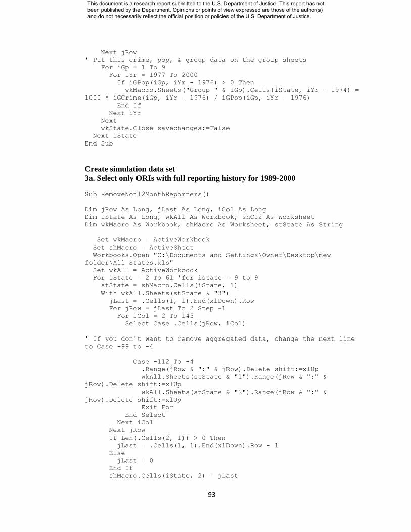
93

Next jRow

' Put this crime, pop, & group data on the group sheets

For iGp = 1 To 9

For iYr = 1977 To 2000

If iGPop(iGp, iYr - 1976) > 0 Then

wkMacro.Sheets("Group " & iGp).Cells(iState, iYr - 1974) =

1000 * iGCrime(iGp, iYr - 1976) / iGPop(iGp, iYr - 1976)

End If

Next iYr

Next

wkState.Close savechanges:=False

Next iState

End Sub

Create simulation data set

3a. Select only ORIs with full reporting history for 1989-2000

Sub RemoveNon12MonthReporters()

Dim jRow As Long, jLast As Long, iCol As Long

Dim iState As Long, wkAll As Workbook, shCI2 As Worksheet

Dim wkMacro As Workbook, shMacro As Worksheet, stState As String



Workbooks.Open "C:\Documents and Settings\Owner\Desktop\new

folder\All States.xls"

Set wkAll = ActiveWorkbook

For iState = 2 To 61 'for istate = 9 to 9

stState = shMacro.Cells(iState, 1)

With wkAll.Sheets(stState & "3")

jLast = .Cells(1, 1).End(xlDown).Row

For jRow = jLast To 2 Step -1

For iCol = 2 To 145

Select Case .Cells(jRow, iCol)

' If you don't want to remove aggregated data, change the next line

to Case -99 to -4

Case -112 To -4

.Range(jRow & ":" & jRow).Delete shift:=xlUp

wkAll.Sheets(stState & "1").Range(jRow & ":" &

jRow).Delete shift:=xlUp

wkAll.Sheets(stState & "2").Range(jRow & ":" &

jRow).Delete shift:=xlUp

Exit For

End Select

Next iCol

Next jRow

If Len(.Cells(2, 1)) > 0 Then

jLast = .Cells(1, 1).End(xlDown).Row - 1

Else

jLast = 0

End If

shMacro.Cells(iState, 2) = jLast


94

End With

Next iState

wkAll.SaveAs "C:\Documents and Settings\Owner\Desktop\new

folder\FullReportingORIs.xls"

wkAll.Close

End Sub

Private Sub GetYearAndMonths(iYr As Long, iMo1 As Long, iMo2 As

Long)

Dim xFreq(1 To 12) As Single

Dim nMos As Long, x As Single

xFreq(1) = 0.5

xFreq(2) = xFreq(1) + 0.08

xFreq(3) = xFreq(2) + 0.02

xFreq(4) = xFreq(3) + 0.05

xFreq(5) = xFreq(4) + 0.02

xFreq(6) = xFreq(5) + 0.18

xFreq(7) = xFreq(6) + 0.02

xFreq(8) = xFreq(7) + 0.02

xFreq(9) = xFreq(8) + 0.03

xFreq(10) = xFreq(9) + 0.01

xFreq(11) = xFreq(10) + 0.01

xFreq(12) = xFreq(11) + 0.06

' Seed the random number generator so you get replicable results

' Change the number to another negative number to change the results

' x = Rnd(-10)

iYr = 1990 + Int(10 * Rnd())

x = Rnd()

Select Case x

Case Is < xFreq(1)

nMos = 1

Case Is < xFreq(2)

nMos = 2

Case Is < xFreq(3)

nMos = 3

Case Is < xFreq(4)

nMos = 4

Case Is < xFreq(5)

nMos = 5

Case Is < xFreq(6)

nMos = 6

Case Is < xFreq(7)

nMos = 7

Case Is < xFreq(8)

nMos = 8

Case Is < xFreq(9)

nMos = 9

Case Is < xFreq(10)

nMos = 10

Case Is < xFreq(11)


95

nMos = 11

Case Is < xFreq(12)

nMos = 12

End Select

' What is the first month of the missing sequence?

x = Rnd()

iMo1 = 1 + Int((13 - nMos) * x)

' What is the last month?

iMo2 = iMo1 + nMos - 1

End Sub

3b. Using the new full reporter data set, select data to be deleted based on the

missingness patterns from step 1.

Sub DeleteData()

Dim stState As String, nDeletions As Long, iState As Long

Dim iDeletion As Long, wkMacro As Workbook, shMacro As Worksheet

Dim wkAll As Workbook, stORI As String, jYr As Long

Dim jMo1 As Long, jMo2 As Long

Dim jRow As Long, jLast As Long, jYrList(1 To 20000) As Long

Dim jRowList(1 To 20000) As Long, jDeletion As Long

Dim jMo1List(1 To 20000) As Long, jMo2List(1 To 20000) As Long

Dim M1 As Long, M2 As Long, iCol As Long, iCol1 As Long, iCol2 As

Long

Dim x As Single, stPath As String

Dim wkState As Workbook, iPg As Long

Dim wkGrp As Workbook, strGrp As String, st2 As String

'x = Rnd(-21509) 'iteration 1





x = Rnd(678) 'iteration 6

stPath = "C:\Users\Marianne\Desktop\new folder\"



Workbooks.Open stPath & "FullReportingORIs.xls"

Set wkAll = ActiveWorkbook

Workbooks.Open stPath & "Longitudinal-5.xls"

Set wkGrp = ActiveWorkbook

wkMacro.Activate




96

With wkAll.Sheets(stState & "3")

If .Cells(2, 1) = "" Then GoTo NextState

jLast = .Cells(1, 1).End(xlDown).Row

nDeletions = 3 * (jLast - 1)

For iDeletion = 1 To nDeletions

ReDo:

jRow = 2 + Int((jLast - 1) * Rnd())

Call GetYearAndMonths(jYr, jMo1, jMo2)

If iDeletion > 1 Then

For jDeletion = 1 To iDeletion - 1

If (jRow = jRowList(jDeletion) And jYr =

jYrList(jDeletion)) Then

M1 = jMo1List(jDeletion) - 1

M2 = jMo2List(jDeletion) + 1

If ((jMo1 - M1) * (M2 - jMo1) >= 0 Or (jMo2 -

M1) * (M2 - jMo2) >= 0) Then

GoTo ReDo

ElseIf ((jMo1 - M1) * (M1 - jMo2) >= 0 Or (jMo1

- M2) * (M2 - jMo2) >= 0) Then

GoTo ReDo

End If

End If

jRowList(iDeletion) = jRow

jYrList(iDeletion) = jYr

jMo1List(iDeletion) = jMo1


Next jDeletion

Else

jRowList(iDeletion) = jRow

jYrList(iDeletion) = jYr



End If

Next iDeletion

End With

' Now to create a new file with the undeleted and deleted data

Workbooks.Add


With wkState

.Sheets.Add after:=.Sheets(3)

.Sheets(4).Name = stState & " FBI"


.Sheets(5).Name = stState & " Longitudinal"

For iPg = 1 To 3

wkAll.Sheets(stState & iPg).Cells.Copy

.Sheets(iPg).Cells(1, 1).PasteSpecial

.Sheets(iPg).Name = stState & iPg

Next iPg

.Sheets(4).Cells(1, 1).PasteSpecial

.Sheets(5).Cells(1, 1).PasteSpecial


.Sheets(6).Name = "Deletions"

With .Sheets(6)


97

.Cells(1, 1) = "Row"

.Cells(1, 2) = "Year"

.Cells(1, 3) = "Month 1"

.Cells(1, 4) = "Month 2"

.Cells(1, 5) = "Group"

.Cells(1, 6) = "State"

.Cells(1, 7) = "Prior Rate"

.Cells(1, 8) = "Current Rate"


.Cells(iDeletion + 1, 1) = jRowList(iDeletion)

.Cells(iDeletion + 1, 2) = jYrList(iDeletion)

.Cells(iDeletion + 1, 3) = jMo1List(iDeletion)

.Cells(iDeletion + 1, 4) = jMo2List(iDeletion)

jRow = jRowList(iDeletion)

jYr = jYrList(iDeletion)

strGrp = Left(wkState.Sheets(stState &

"1").Cells(jRow, jYr - 1828), 1)

.Cells(iDeletion + 1, 5) = Left(strGrp, 1)

st2 = Left(wkState.Sheets(stState & "1").Cells(jRow,

2), 2)

.Cells(iDeletion + 1, 6) = st2

jRow = wkGrp.Sheets("Group " &

strGrp).Range("A:A").Find(st2).Row

.Cells(iDeletion + 1, 7) = wkGrp.Sheets("Group " &

strGrp).Cells(jRow, jYr - 1975)

.Cells(iDeletion + 1, 8) = wkGrp.Sheets("Group " &

strGrp).Cells(jRow, jYr - 1974)

Next iDeletion

End With


iCol1 = 12 * (jYrList(iDeletion) - 1989) +

jMo1List(iDeletion) + 1

iCol2 = 12 * (jYrList(iDeletion) - 1989) +

jMo2List(iDeletion) + 1

For iCol = iCol1 To iCol2

wkState.Sheets(4).Cells(jRowList(iDeletion), iCol) =

-99

wkState.Sheets(4).Cells(jRowList(iDeletion),

iCol).Interior.ColorIndex = 3

wkState.Sheets(5).Cells(jRowList(iDeletion), iCol) =

-99

wkState.Sheets(5).Cells(jRowList(iDeletion),

iCol).Interior.ColorIndex = 3

Next iCol

Next iDeletion

End With

wkState.SaveAs stPath & stState & " Impute"

wkState.Close

NextState:

Next iState

wkAll.Close False

wkGrp.Close False

End Sub

3c. Apply the each imputation method to the simulation data set.


98

Sub ApplyImputations()

stPath = "C:\Users\Marianne\Desktop\new folder\"



Application.ScreenUpdating = False



If shMacro.Cells(iState, 2) = 0 Then GoTo NextState

Workbooks.Open stPath & stState & " Impute.xlsx"


Set shTrue = wkState.Sheets(stState & "3")

Set shFBI = wkState.Sheets(stState & " FBI")

Set shLong = wkState.Sheets(stState & " Longitudinal")

Set shDel = wkState.Sheets("Deletions")

With shDel

nDeletions = .Cells(1, 1).End(xlDown).Row - 1

.Columns("A:H").Select

Application.CutCopyMode = False

.Range("A1:H" & nDeletions + 1).Sort Key1:=Range("A2"),

Key2:=Range("B2"), _

Key3:=Range("C2"), Header:=xlYes

.Range("1:1").Font.Bold = True

End With

' Now do imputing

iDeletion = 1

jLast = shDel.Cells(1, 1).End(xlDown).Row


kRow = shDel.Cells(jRow, 1)

For iYr = 1990 To 2000

If jRow = 17 Then

iDeletion = iDeletion

End If

nMsgMos = 0

nCrPriorYrForMsgMos = 0

nCrPriorYrForRptdMos = 0

nCrThisYr = 0

For iMo = 1 To 12

iCol = 12 * (iYr - 1989) + iMo + 1

xCr = shLong.Cells(kRow, iCol)

If xCr = -99 Then

nMsgMos = nMsgMos + 1

nCrPriorYrForMsgMos = nCrPriorYrForMsgMos +

shLong.Cells(kRow, iCol - 12)

Else

nCrThisYr = nCrThisYr + xCr

nCrPriorYrForRptdMos = nCrPriorYrForRptdMos +

shLong.Cells(kRow, iCol - 12)

End If

Next iMo

Select Case nMsgMos


99

Case 0

Case Is > 9

NextLine

NewGroupImpute

FBIGroupImpute

Case Else

NextLine

NewORIImpute

FBIORIImpute

End Select

Next iYr

Next jRow

' Now calculate the difference(s) between FBI & longitudinal imputation

With shDel

For iCol = 10 To 21

.Cells(1, iCol) = "FBI " & iCol - 9

.Cells(1, iCol + 13) = "Long " & iCol - 9

Next iCol

.Cells(1, 36) = "dYr FBI"

.Cells(1, 37) = "dYr Long"

.Cells(1, 39) = "FBI/N"

.Cells(1, 40) = "Long/N"

For iDeletion = 2 To nDeletions + 1

iCol1 = .Cells(iDeletion, 3)

iCol2 = .Cells(iDeletion, 4)

jRow = .Cells(iDeletion, 1)

jCol = 12 * (.Cells(iDeletion, 2) - 1989) + 1

dYrFBI = 0

dYrLong = 0

xDen = 0

For iCol = iCol1 To iCol2

xTrue = shTrue.Cells(jRow, jCol + iCol)

xDen = xDen + xTrue

x = shFBI.Cells(jRow, jCol + iCol) - xTrue

dYrFBI = dYrFBI + x

.Cells(iDeletion, iCol + 9) = x

x = shLong.Cells(jRow, jCol + iCol) - xTrue

dYrLong = dYrLong + x

.Cells(iDeletion, iCol + 22) = x

Next iCol

.Cells(iDeletion, 36) = dYrFBI

.Cells(iDeletion, 37) = dYrLong

.Cells(iDeletion, 39) = dYrFBI / (iCol2 - iCol1 + 1)

.Cells(iDeletion, 40) = dYrLong / (iCol2 - iCol1 + 1)

Next iDeletion

End With

wkState.Save

wkState.Close

NextState:

Next iState

End Sub


100

Private Sub NewORIImpute()

Dim xChange As Single

If nCrPriorYrForRptdMos > 0 Then

xChange = nCrThisYr / nCrPriorYrForRptdMos

Else

xChange = 1

End If

For iMo = 1 To 12

iCol = 12 * (iYr - 1989) + iMo + 1

If shLong.Cells(kRow, iCol) < -89 Then

shLong.Cells(kRow, iCol) = shLong.Cells(kRow, iCol - 12) *

xChange

shLong.Cells(kRow, iCol).Interior.ColorIndex = 4

' nLong(jRow, iCol) = shLong.Cells(jRow, iCol)

End If

Next iMo

End Sub

Private Sub FBIORIImpute()

Dim xChange As Single

xChange = nCrThisYr / (12 - nMsgMos)

For iMo = 1 To 12

iCol = 12 * (iYr - 1989) + iMo + 1

If shFBI.Cells(kRow, iCol) < -89 Then

shFBI.Cells(kRow, iCol) = xChange

shFBI.Cells(kRow, iCol).Interior.ColorIndex = 4

' nFBI(jRow, iCol) = shFBI.Cells(jRow, iCol - 143)

End If

Next iMo

End Sub

Private Sub NewGroupImpute()

Dim strGrp As String, xRatio As Single

xLastGrpRate = shDel.Cells(iDeletion, 7)

If xLastGrpRate > 0 Then

xRatio = shDel.Cells(iDeletion, 8) / xLastGrpRate

iCol = 12 * (iYr - 1989) + 1

For iMo = 1 To 12

shLong.Cells(kRow, iCol + iMo) = shLong.Cells(kRow, iCol + iMo

- 12) * xRatio

shLong.Cells(kRow, iCol + iMo).Interior.ColorIndex = 4

' nLong(jRow, iCol + iMo) = shLong.Cells(jRow, iCol + iMo)

Next iMo

Else

Exit Sub

End If

End Sub


101

Private Sub FBIGroupImpute()

Dim nPop As Long

xThisGrpRate = shDel.Cells(iDeletion, 8)

If xThisGrpRate > 0 Then

nPop = wkState.Sheets(stState & "1").Cells(kRow, iYr - 1948)

iCol = 12 * (iYr - 1989) + 1

For iMo = 1 To 12

shFBI.Cells(kRow, iCol + iMo) = xThisGrpRate * nPop / 12000

shFBI.Cells(kRow, iCol + iMo).Interior.ColorIndex = 4

' nFBI(jRow, iCol + iMo) = shFBI.Cells(jRow, iCol + iMo)

Next iMo

End If

End Sub

Private Sub NextLine()

With shDel

iDeletion = iDeletion + 1

While .Cells(iDeletion, 1) = .Cells(iDeletion - 1, 1) And

.Cells(iDeletion, 2) = .Cells(iDeletion - 1, 2)

iDeletion = iDeletion + 1

Wend

End With

End Sub


102

APPENDIX D: STATE LEVEL MISSING DATA CHARTS

0%

10%

20%

30%

40%

50%

60%

70%

80%

90%

100%

1977 1979 1981 1983 1985 1987 1989 1991 1993 1995 1997 1999

% o

f M

issi

ng

Dat

a

Alabama

Unweighted Weighted by Population

0%

10%

20%

30%

40%

50%

60%

70%

80%

90%

100%

1977 1979 1981 1983 1985 1987 1989 1991 1993 1995 1997 1999

% o

f M

issi

ng

Dat

a

Alaska



103

0%

10%

20%

30%

40%

50%

60%

70%

80%

90%

100%

1977 1979 1981 1983 1985 1987 1989 1991 1993 1995 1997 1999

% o

f M

issi

ng

Dat

aArizona


0%

10%

20%

30%

40%

50%

60%

70%

80%

90%

100%

1977 1979 1981 1983 1985 1987 1989 1991 1993 1995 1997 1999

% o

f M

issi

ng

Dat

a

Arkansas



104

0%

10%

20%

30%

40%

50%

60%

70%

80%

90%

100%

1977 1979 1981 1983 1985 1987 1989 1991 1993 1995 1997 1999

% o

f M

issi

ng

Dat

aCalifornia


0%

10%

20%

30%

40%

50%

60%

70%

80%

90%

100%

1977 1979 1981 1983 1985 1987 1989 1991 1993 1995 1997 1999

% o

f M

issi

ng

Dat

a

Colorado



105

0%

10%

20%

30%

40%

50%

60%

70%

80%

90%

100%

1977 1979 1981 1983 1985 1987 1989 1991 1993 1995 1997 1999

% o

f M

issi

ng

Dat

aConnecticut


0%

10%

20%

30%

40%

50%

60%

70%

80%

90%

100%

1977 1979 1981 1983 1985 1987 1989 1991 1993 1995 1997 1999

% o

f M

issi

ng

Dat

a

Delaware



106

0%

10%

20%

30%

40%

50%

60%

70%

80%

90%

100%

1977 1979 1981 1983 1985 1987 1989 1991 1993 1995 1997 1999

% o

f M

issi

ng

Dat

aFlorida


0%

10%

20%

30%

40%

50%

60%

70%

80%

90%

100%

1977 1979 1981 1983 1985 1987 1989 1991 1993 1995 1997 1999

% o

f M

issi

ng

Dat

a

Georgia



107

0%

10%

20%

30%

40%

50%

60%

70%

80%

90%

100%

1977 1979 1981 1983 1985 1987 1989 1991 1993 1995 1997 1999

% o

f M

issi

ng

Dat

aHawaii


0%

10%

20%

30%

40%

50%

60%

70%

80%

90%

100%

1977 1979 1981 1983 1985 1987 1989 1991 1993 1995 1997 1999

% o

f M

issi

ng

Dat

a

Idaho



108

0%

10%

20%

30%

40%

50%

60%

70%

80%

90%

100%

1977 1979 1981 1983 1985 1987 1989 1991 1993 1995 1997 1999

% o

f M

issi

ng

Dat

aIllinois


0%

10%

20%

30%

40%

50%

60%

70%

80%

90%

100%

1977 1979 1981 1983 1985 1987 1989 1991 1993 1995 1997 1999

% o

f M

issi

ng

Dat

a

Indiana



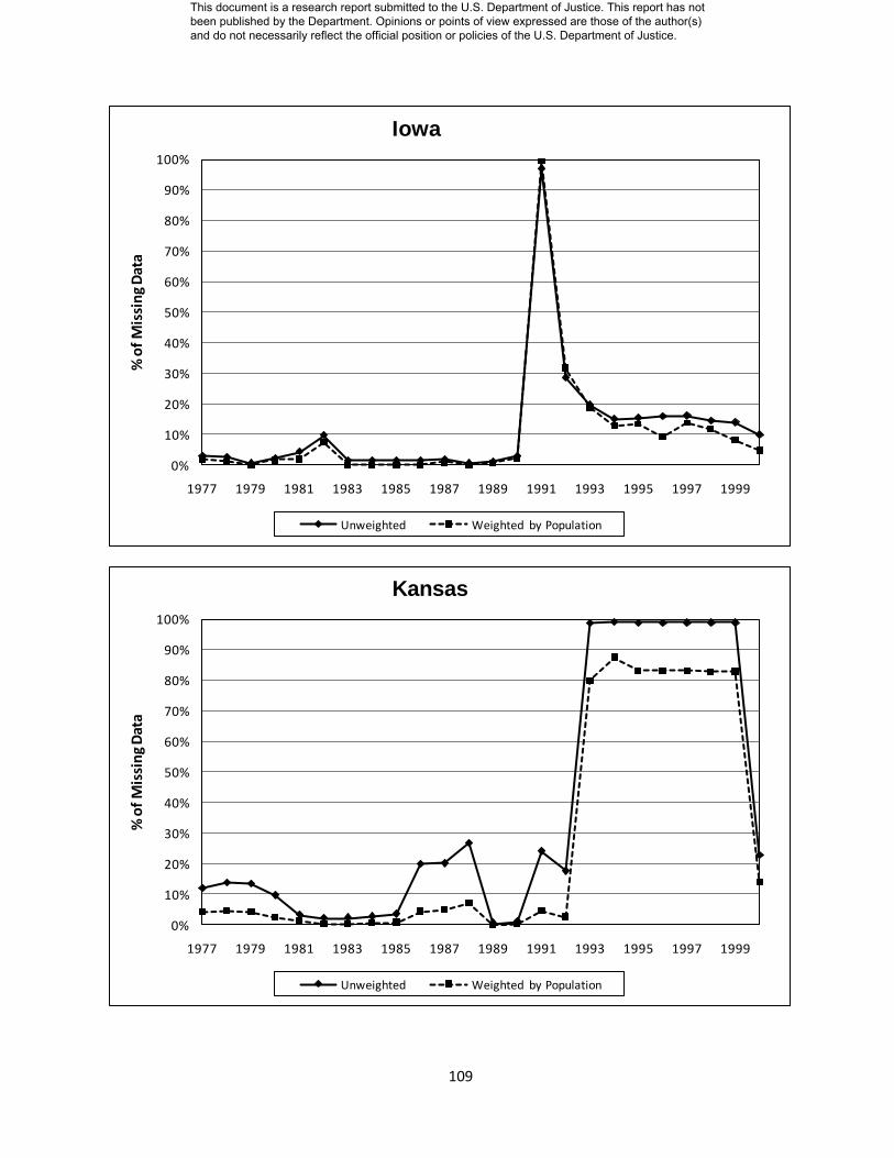
109

0%

10%

20%

30%

40%

50%

60%

70%

80%

90%

100%

1977 1979 1981 1983 1985 1987 1989 1991 1993 1995 1997 1999

% o

f M

issi

ng

Dat

aIowa


0%

10%

20%

30%

40%

50%

60%

70%

80%

90%

100%

1977 1979 1981 1983 1985 1987 1989 1991 1993 1995 1997 1999

% o

f M

issi

ng

Dat

a

Kansas



110

0%

10%

20%

30%

40%

50%

60%

70%

80%

90%

100%

1977 1979 1981 1983 1985 1987 1989 1991 1993 1995 1997 1999

% o

f M

issi

ng

Dat

aKentucky


0%

10%

20%

30%

40%

50%

60%

70%

80%

90%

100%

1977 1979 1981 1983 1985 1987 1989 1991 1993 1995 1997 1999

% o

f M

issi

ng

Dat

a

Louisiana



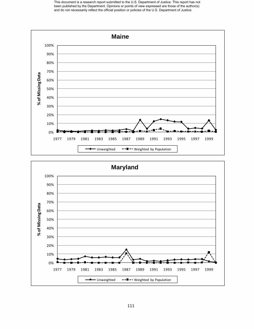
111

0%

10%

20%

30%

40%

50%

60%

70%

80%

90%

100%

1977 1979 1981 1983 1985 1987 1989 1991 1993 1995 1997 1999

% o

f M

issi

ng

Dat

aMaine


0%

10%

20%

30%

40%

50%

60%

70%

80%

90%

100%

1977 1979 1981 1983 1985 1987 1989 1991 1993 1995 1997 1999

% o

f M

issi

ng

Dat

a

Maryland



112

0%

10%

20%

30%

40%

50%

60%

70%

80%

90%

100%

1977 1979 1981 1983 1985 1987 1989 1991 1993 1995 1997 1999

% o

f M

issi

ng

Dat

aMassachusetts


0%

10%

20%

30%

40%

50%

60%

70%

80%

90%

100%

1977 1979 1981 1983 1985 1987 1989 1991 1993 1995 1997 1999

% o

f M

issi

ng

Dat

a

Michigan



113

0%

10%

20%

30%

40%

50%

60%

70%

80%

90%

100%

1977 1979 1981 1983 1985 1987 1989 1991 1993 1995 1997 1999

% o

f M

issi

ng

Dat

aMinnesota


0%

10%

20%

30%

40%

50%

60%

70%

80%

90%

100%

1977 1979 1981 1983 1985 1987 1989 1991 1993 1995 1997 1999

% o

f M

issi

ng

Dat

a

Mississippi



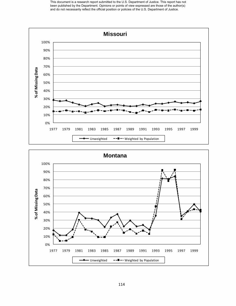
114

0%

10%

20%

30%

40%

50%

60%

70%

80%

90%

100%

1977 1979 1981 1983 1985 1987 1989 1991 1993 1995 1997 1999

% o

f M

issi

ng

Dat

aMissouri


0%

10%

20%

30%

40%

50%

60%

70%

80%

90%

100%

1977 1979 1981 1983 1985 1987 1989 1991 1993 1995 1997 1999

% o

f M

issi

ng

Dat

a

Montana



115

0%

10%

20%

30%

40%

50%

60%

70%

80%

90%

100%

1977 1979 1981 1983 1985 1987 1989 1991 1993 1995 1997 1999

% o

f M

issi

ng

Dat

aNebraska


0%

10%

20%

30%

40%

50%

60%

70%

80%

90%

100%

1977 1979 1981 1983 1985 1987 1989 1991 1993 1995 1997 1999

% o

f M

issi

ng

Dat

a

Nevada



116

0%

10%

20%

30%

40%

50%

60%

70%

80%

90%

100%

1977 1979 1981 1983 1985 1987 1989 1991 1993 1995 1997 1999

% o

f M

issi

ng

Dat

aNew Hampshire


0%

10%

20%

30%

40%

50%

60%

70%

80%

90%

100%

1977 1979 1981 1983 1985 1987 1989 1991 1993 1995 1997 1999

% o

f M

issi

ng

Dat

a

New Jersey



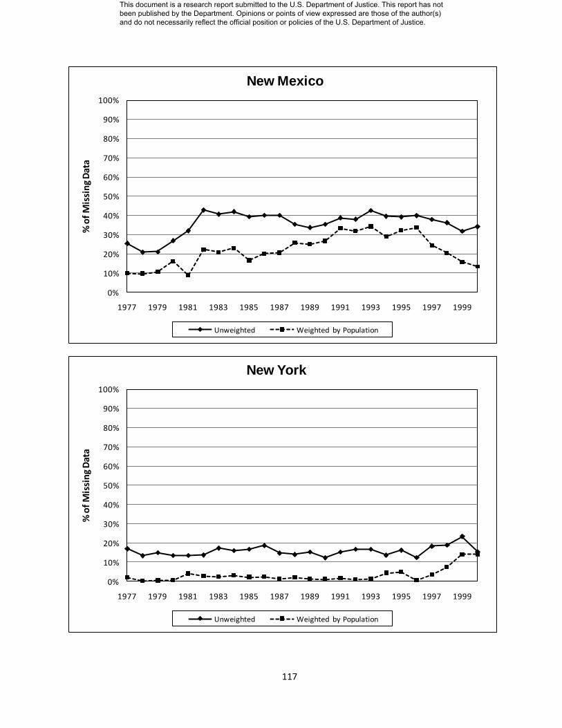
117

0%

10%

20%

30%

40%

50%

60%

70%

80%

90%

100%

1977 1979 1981 1983 1985 1987 1989 1991 1993 1995 1997 1999

% o

f M

issi

ng

Dat

aNew Mexico


0%

10%

20%

30%

40%

50%

60%

70%

80%

90%

100%

1977 1979 1981 1983 1985 1987 1989 1991 1993 1995 1997 1999

% o

f M

issi

ng

Dat

a

New York



118

0%

10%

20%

30%

40%

50%

60%

70%

80%

90%

100%

1977 1979 1981 1983 1985 1987 1989 1991 1993 1995 1997 1999

% o

f M

issi

ng

Dat

aNorth Carolina


0%

10%

20%

30%

40%

50%

60%

70%

80%

90%

100%

1977 1979 1981 1983 1985 1987 1989 1991 1993 1995 1997 1999

% o

f M

issi

ng

Dat

a

North Dakota



119

0%

10%

20%

30%

40%

50%

60%

70%

80%

90%

100%

1977 1979 1981 1983 1985 1987 1989 1991 1993 1995 1997 1999

% o

f M

issi

ng

Dat

aOhio


0%

10%

20%

30%

40%

50%

60%

70%

80%

90%

100%

1977 1979 1981 1983 1985 1987 1989 1991 1993 1995 1997 1999

% o

f M

issi

ng

Dat

a

Oklahoma



120

0%

10%

20%

30%

40%

50%

60%

70%

80%

90%

100%

1977 1979 1981 1983 1985 1987 1989 1991 1993 1995 1997 1999

% o

f M

issi

ng

Dat

aOregon


0%

10%

20%

30%

40%

50%

60%

70%

80%

90%

100%

1977 1979 1981 1983 1985 1987 1989 1991 1993 1995 1997 1999

% o

f M

issi

ng

Dat

a

Pennsylvania



121

0%

10%

20%

30%

40%

50%

60%

70%

80%

90%

100%

1977 1979 1981 1983 1985 1987 1989 1991 1993 1995 1997 1999

% o

f M

issi

ng

Dat

aRhode Island


0%

10%

20%

30%

40%

50%

60%

70%

80%

90%

100%

1977 1979 1981 1983 1985 1987 1989 1991 1993 1995 1997 1999

% o

f M

issi

ng

Dat

a

South Carolina



122

0%

10%

20%

30%

40%

50%

60%

70%

80%

90%

100%

1977 1979 1981 1983 1985 1987 1989 1991 1993 1995 1997 1999

% o

f M

issi

ng

Dat

aSouth Dakota


0%

10%

20%

30%

40%

50%

60%

70%

80%

90%

100%

1977 1979 1981 1983 1985 1987 1989 1991 1993 1995 1997 1999

% o

f M

issi

ng

Dat

a

Tennessee



123

0%

10%

20%

30%

40%

50%

60%

70%

80%

90%

100%

1977 1979 1981 1983 1985 1987 1989 1991 1993 1995 1997 1999

% o

f M

issi

ng

Dat

aTexas


0%

10%

20%

30%

40%

50%

60%

70%

80%

90%

100%

1977 1979 1981 1983 1985 1987 1989 1991 1993 1995 1997 1999

% o

f M

issi

ng

Dat

a

Utah



124

0%

10%

20%

30%

40%

50%

60%

70%

80%

90%

100%

1977 1979 1981 1983 1985 1987 1989 1991 1993 1995 1997 1999

% o

f M

issi

ng

Dat

aVermont


0%

10%

20%

30%

40%

50%

60%

70%

80%

90%

100%

1977 1979 1981 1983 1985 1987 1989 1991 1993 1995 1997 1999

% o

f M

issi

ng

Dat

a

Virginia



125

0%

10%

20%

30%

40%

50%

60%

70%

80%

90%

100%

1977 1979 1981 1983 1985 1987 1989 1991 1993 1995 1997 1999

% o

f M

issi

ng

Dat

aWashington


0%

10%

20%

30%

40%

50%

60%

70%

80%

90%

100%

1977 1979 1981 1983 1985 1987 1989 1991 1993 1995 1997 1999

% o

f M

issi

ng

Dat

a

West Virginia



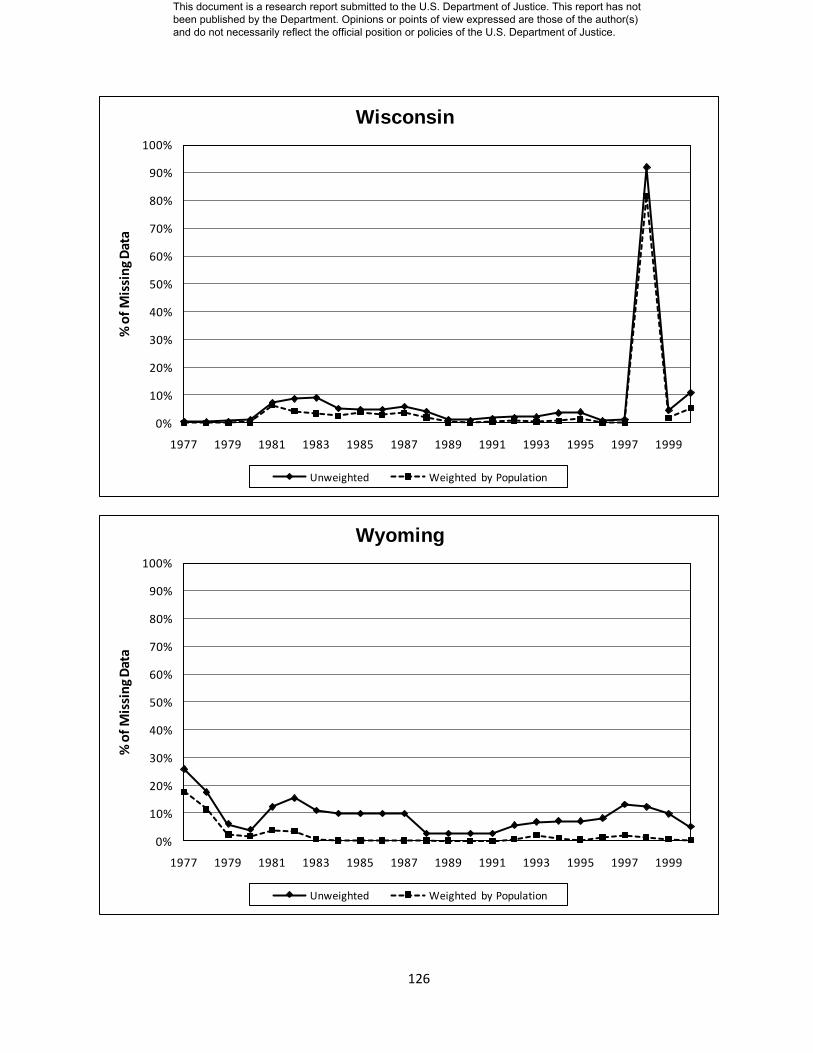
126

0%

10%

20%

30%

40%

50%

60%

70%

80%

90%

100%

1977 1979 1981 1983 1985 1987 1989 1991 1993 1995 1997 1999

% o

f M

issi

ng

Dat

aWisconsin


0%

10%

20%

30%

40%

50%

60%

70%

80%

90%

100%

1977 1979 1981 1983 1985 1987 1989 1991 1993 1995 1997 1999

% o

f M

issi

ng

Dat

a

Wyoming



127

CITED LITERATURE

Addington, L. (2004). "The Effect of NIBRS Reporting on Item Missing Data in Murder Cases."

Homicide Studies 8(3): 193-213.

Akiyama, Y. and S. K. Propheter (2005). Methods of Data Quality Contol: For Uniform Crime

Reporting Programs. Clarksburg, WV, Criminal Justice Informaiton Services Division, Federal

Bureau of Investigation.

Black, D. J. (1970). "Production of Crime Rates." American Sociological Review 35: 733-758.

Blumstein, A., J. Cohen, et al. (1992). "The UCR-NCS Relationship Revisitied: A Reply to

Menard." Criminology 30(1): 115-124.

Brame, R. and R. Paternoster (2003). "Missind Data Problems in Criminological Research: Two

Case Studies." Journal of Quantitative Criminology 19(1): 55-78.

Brownstein, H. H. (2000). "The Social Production of Crime Statistics." Justice Research and

Policy 2(2): 73-89.

Cleveland, W. S. (1993). Visualizing Data. Murray Hill, NJ, AT&T Bell Laboratories.

Cleveland, W. S. (1994). The Elements of Graphing Data. Murray Hill, NJ, AT&T Bell

Laboratories.

Conaway, M. R. and S. L. Lohr (1994). "A Longitudinal Analysis of Factors Associated with

Reporting Violence Crimes to the Police." Journal of Quantitative Criminology 10(1): 23-39.

Dorinski, S. M. (1998). "Imputation Methods in the Sample Survey of Law Enforcement

Agencies." American Statistical Association Proceedings on Survey Research: 302-307.

FBI (1966). Uniform Crime Reporting Handbook. Washington, D.C., U.S. Department of

Justice.

FBI (1984). Uniform Crime Reporting Handbook. Washington, D.C., U.S. Department of

Justice.

FBI (1999). Hate Crime Data Collection Guidelines. Washington, D.C., U.S. Department of

Justice.

FBI (2000). National Incident-Based Reporting System, Volume 1, Data Collection Guidelines.

Washington, DC, US Department of Justice.

FBI (2002). Uniform Crime Reporting Program Data [United States]: 1977-2000 [Computer

file]. ICPSR09028, Inter-university Consortium for Political and Social Research [distributor],

Ann Arbor, MI.


128

FBI (2007). Crime in the United States. Washington, DC, US Department of Justice.

FBI (2011). "NIBRS General FAQs." Retreived from http://www.fbi.gov/about-

us/cjis/ucr/frequently-asked-questions/nibrs_faqs#agencyparticipation on 4/15/2011.

Flewelling, R. L. (2004). "A Nonparametric Imputation Approach for Dealing With Missing

Variables in SHR Data." Homicide Studies 8(3): 255-266.

Fox, J. A. (2000). Demographics and U.S. Homicide. The Crime Drop in America. A. Blumstein

and J. Wallman. New York, Cambridge University Press.

Fox, J. A. (2004). "Missing Data Problems in the SHR." Homicide Studies 8(3): 214-254.

Jacobs, J. and K. Potter (1998). Hate Crimes: Criminal Law and Identity Politics. New York,

NY, Oxford University Press.

Kituse, J. L. and A. V. Cicourel (1963). "A Note on the Uses of Official Statistics." Social

Problems 11: 131-139.

Kposowa, A. J., K. D. Breault, et al. (1995). "Reassessing the structural covariates of violent and

property crimes in the USA: A county level analysis." British Journal of Sociology 46: 79-105.

LaFree, G. (1989). Rape and Criminal Justice: The Social Construction of Sexual Assault.

Belmont, CA, Wadsworth, Inc.

Lillard, L., J. P. Smith, et al. (1986). "What Do We Really Know About Wages? The Importance

of Nonreporting and Census Imputation." Journal of Political Economy 94(3): 489-506.

Little, R. J. A. (1988). "Missing-Data Adjustments in Large Surveys." Journal of Business &

Economic Statistics 6(3): 287-296.

Little, R. J. A. and D. B. Rubin (1987). Statitical Analysis of Missing Data. New York, John

Wiley & Sons.

Little, R. J. A. and D. B. Rubin (1989). "The Analysis of Social Science Data with Missing

Values." Sociological Methods and Research 18(2&3): 292-326.

Little, R. J. A. and H.-L. Su (1989). Item Nonresponse in Panel Surveys. Panel Surveys. D.

Kasprzyk, G. Duncan, G. Kalton and M. P. Singh. New York, John Wiley & Sons.

Loftin, C. (1986). "The Validity of Robbery-Murder Classifications in Baltimore." Violence and

Victims 1(3): 191-205.

Loftin, C., D. McDowall, et al. (2008). "A Comparison of SHR and Vital Statistics Homicide."

Journal of Contemporary Criminal Justice 24(1): 4-17.


http://www.fbi.gov/about-us/cjis/ucr/frequently-asked-questions/nibrs_faqs#agencyparticipation

http://www.fbi.gov/about-us/cjis/ucr/frequently-asked-questions/nibrs_faqs#agencyparticipation

129

Lott, J. R. (1998). More Guns, Less Crime. Chicago, IL, University of Chicago Press.

Lott, J. R. (2000). More Guns, Less Crime. Chicago, IL, University of Chicago Press.

Lott, J. R. and D. B. Mustard (1997). "Crime, Deterrence, and Right-to-Carry Concealed

Handguns." Journal of Legal Studies 26: 1-68.

Lynch, J. P. and L. A. Addington (2007). Understanding Crime Statistics: Revisiting the

Divergence of the NCVS and UCR. Cambridge, MA, Cambridge University Press.

Lynch, J. P. and J. P. Jarvis (2008). "Missing Data and Imputation in Uniform Crime Reports

and the Effects on National Estimates." Journal of Contemporary Criminal Justice 24(1): 69-85.

Maisel, R. and C. H. Persell (1996). How Sampling Works. Thousand Oaks, CA, Pine Forge

Press.

Maltz, M. D. (1977). "Crime Statistics: A Historical Perspective." Crime and Delinquency 23(1):

32-40.

Maltz, M. D. (1998). "Visualizing Homicide: A Research Note." Journal of Quantitative

Criminology 15(4): 397-410.

Maltz, M. D. (1998). "Which Homicides Decreased? Why?" Journal of Criminal Law and

Criminology 88(4): 1479-1486.

Maltz, M. D. (1999). Bridging Gaps in Police Crime Data. Washington D.C., Bureau of Justice

Statistics.

Maltz, M. D. (2006). Missing UCR Data and Divergence of the NCVS and UCR Trends. J. P. a.

A. Lynch, Lynn.

Maltz, M. D. (2007). Missing UCR Data and Divergence of the NCVS and UCR Trends.

Understanding Crime Statistics: Revisting the Divergence of the NCVS and UCR. J. P. Lynch

and L. A. Addington. New York, NY, Cambridge University Press: 269-298.

Maltz, M. D., Ed. (2009). Look Before You Analyze: Visualizing Data in Criminal Justice.

Handbook of Quantiative Criminology. New York, NY, Springer.

Maltz, M. D. and J. Targonski (2002). "A Note on the Use of County-Level Data." Journal of

Quantitative Criminology 18(3): 297-318.

Maltz, M. D. and J. Targonski (2003). "Measurement and Other Errors in County-Level UCR

Data: A Reply to Lott and Whitley." Journal of Quantitative Criminology 19(2): 199-206.


130

Maxfield, M. G. (1989). "Circumstances in Supplementary Homicide Reports: Variety and

Validity." Criminology 27(4): 671-695.

McCleary, R., B. C. Nienstedt, et al. (1982). "Uniform Crime Reports as Organizational

Outcomes: Three Time Series Experiments." Social Problems 29(4): 361-372.

Menard, S. (1991). "Encouraging News for Criminologists (In the Year 2050)?: A Comment on

O'Brien (1990)." Journal of Criminal Justice 19: 563-567.

Menard, S. (1992). "Residual Gains, Reliability, and the UCR-NCS Relationship: A Comment

on Blumstein, Cohen, and Rosenfeld (1991)." Criminology 30(1): 105-113.

Mosher, C. J., T. D. Miethe, et al. (2002). The Mismeasure of Crime. Thousand Oaks, CA, Sage.

Nolan, J., S. M. Hass, et al. (2006). "Establishing the "Statistical Accuracy" of Uniform Crime

Reports (UCR) in West Virginia." State of West Virginia, Division of Criminal Justice.

O'Brien, R. M. (1990). "Comparing Detrended UCR and NCS Crime Rates Over Time: 1973-

1986." Journal of Criminal Justice 18: 229-238.

O'Brien, R. M. (1991). "Detrended UCR and NCS Crime Rates: Their Utility and Meaning."

Journal of Criminal Justice 19: 569-574.

Petee, T. A. and G. S. Kowalski (1993). "Modeling Rural Violent Crime Rates: A Test of Social

Disorganization Theory." Sociological Focus 28(1): 87-89.

Petee, T. A., G. S. Kowalski, et al. (1994). "Crime, social disorganization, and social structure: A

research note on the use of interurban ecological models." American Journal of Criminal Justice

19: 117-127.

Poggio, E. C., Kennedy, Stephen D., Chaiken, Jan M., Carlson, Kenneth E. (1985). "Blueprint

for the Future of the Uniform Crime Reporting Program." US Department of Justice: FBI.

Pridemore, W. A. (2005). "A Cautionary Note on Using County-Level Crime and Homicide

Data." Homicide Studies 9(3): 256-268.

Queally, J. and D. Giambusso (2010). "More than 200 Newark police officers may face layoffs

due to $16.7M budget shortfall." Retrieved from

http://www.nj.com/news/index.ssf/2010/07/more_than_200_newark_police_of.html on

3/15/2011.

Riedel, M. (1990). Nationwide Homicide Data Sets: An Evaluation of the Uniform Crime

Reports and the National Center for Health Statistics Data. Measuring Crime: Large-Scale,

Long-Range Efforts. D. L. MacKenzie, P. J. Baunach and R. R. Roberg. Albany, NY, State

University of New York Press.


http://www.nj.com/news/index.ssf/2010/07/more_than_200_newark_police_of.html

131

Riedel, M. and W. C. Regoeczi (2004). "Missing Data In Homicide Research." Homicide Studies

8(3): 163-192.

Ringel, C. (1997). Criminal Victimization 1996. Washington, D.C., U.S. Department of Justice.

Rosenbaum, D. P. (1987). "Coping with Victimization: The Effects of Police Intervention On

Victim's Psychological Readjustment." Crime and Delinquency 33(4): 502-519.

Rubin, D. B. (1987). Multiple Imputation for Nonresponse in Surveys. New York, John Wiley &

Sons.

Rubin, D. B. (1996). "Multiple Imputation After 18+ Years." Journal of the American Statistical

Association 91(434): 473-489.

Schafer, J. L. and J. W. Graham (2002). "Missing Data: Our View of the State of the Art."

Psychological Methods 7(2): 144-177.

Schneider, V. W. and B. Wiersema (1990). Limits and Use of the Uniform Crime Reports.

Measuring Crime: Large-Scale, Long-Range Efforts. D. L. MacKenzie, P. J. Baunach and R. R.

Roberg. Albany, NY, State University of New York Press.

Seidman, D. and M. Couzens (1974). "Getting the Crime Rate Down: Political Pressure and

Crime Reporting." Law and Society Review 8: 457-493.

Sherman, L. W., D. Gottfredson, et al. (1997). Preventing Crime: What Works, What Doesn't,

What's Promosing. College Park, MD, Department of Criminology and Criminal Justice,

Univerisy of Maryland.

Shon, P. and J. Targonski (2003). "Declining Trends in U.S. Parricides, 1976-1998."

International Journal of Law and Psychiatry 387: 1-16.

Skogan, W. G. (1974). "The Validity of Official Crime Statistics: An Empirical Investigation."

Social Science Quarterly 55: 25-38.

Skogan, W. G. (1975). "Measurement Problems in Official and Survey Crime Rates." Journal of

Criminal Justice 3: 17-32.

Skogan, W. G. (1977). "Dimensions of the Dark Figure of Unreported Crime." Crime and

Delinquency 23(1): 41-50.

Tremblay, A. (1994). Longitudinal Imputation of SIPP Food Stamp Benefits. Washington, DC,

U.S. Bureau of the Census.

Tufte, E. R. (1983). The Visual Display of Quantitative Information. Cheshire, CT, Graphics

Press.


132

Tufte, E. R. (1990). Envisioning Information. Cheshire, CT, Graphics Press.

Tufte, E. R. (1997). Visual Explanations. Cheshire, CT, Graphics Press.

Ullman, S. E. and J. M. Siegel (1994). "Predictors of Exposure to Traumatic Events and

Posttraumatic Stress Sequelae." Journal of Community Psychology 22: 328-338.

User Technology Associates, I., Ed. (1999). CJIS Crime Reporting (CCR) Project: Refined

Quality Control, Imputation and Estimation Algorithms and Detailed, Tutorial Documentation of

Algorithms for Oversight Committees. Arlington, VA.

Van Court, J. and R. B. Trent (2004). "Why Didn't We Get Them All?" Homicide Studies 8(3):

311-321.

Wadsworth, T., J. M. Roberts, et al. (2008). "When Missing Data are Not Missing: A New

Approach to Evaluating Supplemental Homicide Report Imputation Strategies." Criminology

46(4): 841-870.

Wilkinson, K. P. (1984). "Rurality and Patterns of Social Disruption." Rural Sociology 49(1):

23-36.

Williams, T. R. and L. Bailey (1996). "Compensating for Missing Wave Data in the Survey of

Income and Program Participation (SIPP)." American Statistical Association Proceedings on

Survey Research: 305-310.

Yansaneh, I. S., L. S. Wallace, et al. (1998). "Imputation Methods for Large Complex Datasets:

An Application to the NEHIS." American Statistical Association Proceedings on Survey

Research: 314-319.

Ybarra, L. M. R. and S. L. Lohr (2002). "Estimates of repeat victimization using the National

Crime Victimization Survey." Journal of Quantitative Criminology 18: 1-22.


133

VITA

Joseph Robert Targonski University of Illinois at Chicago

Department of Criminology, Law and Justice

1007 West Harrison (M/C 141)

Chicago, IL 60607-7140

(312) 413-5893

E-mail: [email protected]

Research Interests: Crime measurement, UCR Data, Imputation, gun violence.

Education: Doctor of Philosophy in Criminology, Law, and Justice (Expected 8/2011)

University of Illinois at Chicago

Dissertation: “A Comparison of Imputation Methodologies in the Offenses-

Known Uniform Crime Reports”

Chair: Dr. Michael D. Maltz

Master of Arts in Criminal Justice, 5/2001

University of Illinois at Chicago

Bachelor of Arts in Sociology, 5/1999

University of Colorado at Boulder

Thesis: “Fear of Crime: Examining Gender Differences in the Context of Other

Independent Variables,”

Chair: Dr. Joanne Belknap

Cumulative GPA: 3.25/4.0

Major GPA: 3.76/4.0

Experience: Data Investigation Manager 3/2007-Present

Information Resources, Inc. Chicago, IL

Promotion Analyst, 5/2006-3/2007

NCH Marketing Services, Inc. Deerfield, IL

Data Investigation Analyst, 6/2003-5/2006

Information Resources, Inc. Chicago, IL


134

Research Assistant, 1/2000-6/2003

Dr. Michael D. Maltz, University of Illinois-Chicago

Co-Principal Investigator for NIJ Grant, “Enhancing Imputation Methodologies

for County-Level UCR Data”

Examine patterns of missing UCR data to develop longitudinal imputation

procedures

Teaching Assistant, 8/2001-12/2001

Criminal Justice 262, Statistics, University of Illinois-Chicago

Dr. Michael D. Maltz


Dr. Mindie Lazarus-Black, University of Illinois-Chicago

Entered court record data for domestic violence cases in the Caribbean

Maintained the quality of database and coordinated project efforts with principal

investigators


Center for the Prevention of Adverse Life Outcomes, Boulder, CO.

Trained and supervised approximately 15 lab staff

Developed and maintained a database for juvenile arrest records

Collected and analyzed interview data from juvenile offenders

Honors and

Activities: Recipient of the $20,000 2004 National Institute of Justice Graduate Research Fellowship

$15,000 University Fellowship, University of Illinois at Chicago, 8/2002-8/2003

Member of American Statistical Association’s Crime and Justice UCR Subcommittee,

4/2002-Present

$2,500 award from Bureau of Justice Statistics to attend ICPSR workshop, “Quantitative

Analysis of Crime and Criminal Justice,” 6/2001, University of Michigan at Ann Arbor.

“Missing Data: Statistical Analysis of Data with Incomplete Observations,” 7/2002,

ICPSR summer course, University of Michigan at Ann Arbor.

$350 Graduate Student Council Travel Award, 11/2001

$200 Graduate College Travel Award, 10/2001

$175 Graduate College Travel Award, 4/2001


135

$250 Graduate Student Council Travel Award, 11/2000

Chicago Bar Association Entertainment Committee Criminal Justice Graduate Award

Recipient, 4/2000 and 4/2002

Graduated Cum Laude, University of Colorado at Boulder

Dean’s List, Spring 1998, Fall 1998, and Spring 1999

University of Colorado at Boulder

Psi Chi, The National Honor Society in Psychology, 2/1997-Present

Alpha Kappa Delta, The National Honor Society in Sociology,

10/1998 –Present

Professional

Societies: American Society of Criminology

Academy of Criminal Justice Sciences

Justice Research and Statistics Association

Homicide Research Working Group

American Statistical Association

Publications:

Shon, Phillip C.H., Sudipto Roy, and Joseph Targonski (2007) “Female Offender

Parricides: The Asymmetrical Distribution of Homicide for Parents ad Stepparents,”

Criminology and Social Integration, 14 (2): 13-23.

Shon, Phillip and Joseph Targonski (2003). “Declining Trends in U.S. Parricides, 1976-

1998,” International Journal of Law and Psychiatry, 387: 1-16.

Maltz, Michael D. and Joseph Targonski (2003) “Measurement and Other Errors in

County-Level UCR Data: A Reply to Lott and Whitley,” Journal of Quantitative

Criminology 19(2): 199-206.

Maltz, Michael D. and Joseph Targonski (2002) “A Note on the Use of County-Level

UCR Data” Journal of Quantitative Criminology, 18(3): 297-318.

Chaiken, Marcia R., Boland, Barbara, Maltz, Michael, Martin, Susan, and Joseph

Targonski (2001). “State and Local Change and the Violence Against Women Act,” NIJ

Research Report, NCJ 191186, Washington, D.C.


136

Presentations:

“Missing in Action: Handling Agency Nonresponse in the UCR.” (with Michael Maltz).

2003 Annual Meeting of the American Society of Criminology, Denver, CO.

“Normal Beginnings: John Hinckley and Timothy McVeigh.” (with Jeffery Frost).

Presidential Panel on “Visualizing Life Course Trajectories,” 2002 Annual Meeting of

the American Society of Criminology, Chicago, IL.

“Life Course Visualization methodology,” (with Sharon Shipinski, and Marianne Ring),

2001 Annual Meeting of the Homicide Research Working Group, St. Louis, MO.

“Fear of Crime and Social Control: A Community-Level Analysis Across 100

Neighborhoods,” (with Dennis Rosenbaum), 2001 Annual Meeting of the American

Society of Criminology, Atlanta, GA.

“Dealing with Missing Data in the UCR,” (with Michael Maltz), 2001 Annual Meeting of

the Justice Research and Statistics Association, New Orleans, LA.

“Trends in U.S. Parricides, 1976-1998,” (with Phillip Shon), 2001 Annual Meeting of the

Academy of Criminal Justice Sciences, Washington, D.C.

“Imputation Issues in UCR Data,” (with Michael D. Maltz), 2000 Annual Meeting of the

American Society of Criminology, San Francisco, CA.

“Gender and Fear of Crime: Explaining the Discrepancy in Relation to Victimization

Rates,” 1999 Annual Meeting of the Midwest Sociological Society, Minneapolis, MN.

(Queally and Giambusso 2010)

(User Technology Associates 1999; FBI 2002; Akiyama and Propheter 2005)
