a comparison o methodf s of determining the …
TRANSCRIPT
A COMPARISON OF METHODS OF DETERMINING THE ALLOWABLE CUT
ON THE UNIVERSITY OF BRITISH COLUMBIA RESEARCH FOREST,
HANEY, B. C.
by
Miklos Kovats B.S.F., University of British Columbia (Sopron Division), 1958
A THESIS SUBMITTED IN PARTIAL FULFILMENT OF
THE REQUIREMENTS FOR THE DEGREE OF
MASTER OF FORESTRY
in the Department of
FORESTRY
We accept this thesis as conforming to the
required standard
THE UNIVERSITY OF BRITISH COLUMBIA
January, 1962

In present ing t h i s thes i s i n p a r t i a l f u l f i l m e n t o f
the requirements f o r an advanced degree at the Un i ve r s i t y of
B r i t i s h Columbia, I agree tha t the L i b r a r y s h a l l make i t f r e e l y
ava i l ab l e f o r reference and study. I f u r the r agree that permission
f o r extensive copying of t h i s t h e s i s f o r s cho l a r l y purposes may be
granted by the Head of my Department or by h i s representa t i ves .
It i s understood tha t copying or pub l i c a t i on of t h i s thes i s f o r
f i n a n c i a l ga in s h a l l not be alloiired without my wr i t ten permiss ion.
Department of Forestry
The Un i ve r s i t y of B r i t i s h Columbia, Vancouver 8, Canada.
Date January 30 > 1962

i i
ABSTRACT
A COMPARISON OF METHODS OF DETERMINING THE ALLOWABLE CUT ON THE
UNIVERSITY OF BRITISH COLUMBIA RESEARCH FOREST, HANEY, B. C.
Generally i t i s not adequate to calculate an allowable cut
for a property by only one formula or method. Usually i t is
preferable to u t i l i z e a l l the information available with as
many suitable formulae or methods as possible to obtain reason
able estimates of the yearly u t i l i z a t i o n rates by several
approaches.
For the University Research Forest fifteen different
formulae and methods were selected for comparison, because their
basic assumptions appeared applicable to this forest. The
methods and formulae tested were:
Methods: Area regulation, Area-volume check, Area-volume
allotment, Barnes1 and H. A. Meyer's.
Formulae: Austrian, Black H i l l s , Grosenbaugh, Hanzlik,
Hundeshagen, Kemp, W. H. Meyer, S. Petrini (compound and simple
interest) and Von Mantel.
Appropriate inventory techniques were developed in order
to collect the necessary information regarding rates of growth,
mortality and numbers of trees per acre by diameter classes.
Present and future decadal growing stocks were estimated.
Simple and compound growth rates, including and excluding

i i i
ingrowth, for a l l types were calculated separately for stands
over eighty years of age and for stands under eighty years.
The inventory was based on the areas and estimates taken from
1961 aerial photographs supplemented by both temporary and
permanent sample plots, employing primarily the principles of
the point sampling techniques as described by L. R. Grosenbaugh.
After substituting the actual data into the formulae and
various methods, allowable cut estimates for 3.1, 9.1, 11.1,
and 13.1 inches minimum diameter limits were calculated.
Allowances were made for an intermediate standard of u t i l i z a
tion and for waste, breakage and decay.
Considering the inventory and the allowable cut calcula
tions i t was found that:
1. Simple area regulation w i l l lead to undesirably large
fluctuations in allowable cut.
2. Volume formulae are useful means of determining the
yearly harvest volume, though the distribution of the cut on
the ground requires definition in terms of area as well.
3. Neither area nor volume control can be used exclusively.
Some combination and integration is usually necessary in actual
practice. In the case of the Research Forest this can be
applied most conveniently by following the area-volume computa
tion basis.
i v
TABLE OF CONTENTS
Page
INTRODUCTION 1
METHODS OF CALCULATING THE ALLOWABLE CUT 5
AREA CONTROL 5
VOLUME CONTROL 6
AREA AND VOLUME CONTROL 7
DESCRIPTION OF METHODS USED 8
AREA CONTROL METHODS 8
AREA REGULATION 8
VOLUME CONTROL METHODS 9
HANZLIK'S FORMULA 9
AUSTRIAN FORMULA 9
KEMP'S FORMULA 10
BARNES1 METHOD 12
BLACK HILLS FORMULA 12
HUNDESHAGEN'S FORMULA 13
VON MANTEL'S FORMULA 14
S. PETRINI'S COMPOUND INTEREST FORMULA 15
S. PETRINI'S SIMPLE INTEREST FORMULA 16
W. H. MEYER'S AMORTIZATION FORMULA 16
GROSENBAUGH'S SIMPLE INTEREST FORMULA 17
H. A. MEYER'S METHOD 18
Page
AREA AND VOLUME CONTROL METHODS 19
AREA-VOLUME COMPUTATION 19
AREA-VOLUME ALLOTMENT 22
NECESSARY INFORMATION 24
DATA COLLECTION AND CALCULATION METHODS 25
CLASSIFICATION 25
AGE CLASS LIMITS 25.
FOREST TYPES 25
SITE CLASSES 26
DIAMETER CLASSES 26
THE USE OF AERIAL PHOTOGRAPHS 27
PHOTO TYPING 27
PHOTOGRAPHIC HEIGHT MEASUREMENTS 27
AREA DETERMINATION 31
THE USE OF McBEE PUNCH CARDS 37
GROUND SAMPLING 41
METHOD OF CALCULATING THE NUMBER OF TREES PER ACRE
AND MORTALITY RATES 4 4
METHOD OF CALCULATING FUTURE DIAMETER GROWTH 52
STAND TABLE PROJECTIONS 56
ROTATION AGE 59
MISCELLANEOUS CALCULATIONS 5 9

v i
Page
ALLOWABLE CUT CALCULATIONS 65
AREA REGULATION 65
VOLUME CONTROL FORMULAE 70
AUSTRIAN FORMULA 70
HANZLIK'S FORMULA 71
KEMP'S FORMULA 72
BARNES' METHOD 74
BLACK HILLS FORMULA 76
HUNDESHAGEN'S FORMULA 77
H. A. MEYER'S METHOD 78
VON MANTEL'S FORMULA 81
GROSENBAUGH'S SIMPLE INTEREST FORMULA 81
W. H. MEYER'S AMORTIZATION FORMULA 83
S. PETRINI'S COMPOUND INTEREST FORMULA 83
S. PETRINI'S SIMPLE INTEREST FORMULA 84
AREA AND VOLUME CONTROL METHODS 85
AREA-VOLUME COMPUTATION 85
AREA-VOLUME ALLOTMENT 88
CONCLUSION 92
BIBLIOGRAPHY 101

v i i
LIST OF TABLES
Number Page
1. WEIGHTS OF POINTS BY ELEVATION LIMITS 33
2. COMPARISON OF AREAS AS ESTIMATED IN 1958 AND 1961 34
3. AREA SUMMARY FOR THE UNIVERSITY RESEARCH FOREST 35
4. COMPARISON OF PRODUCTIVE AREAS AS ESTIMATED IN 1958
AND 1961 36
5. SITE INDICES AND CORRESPONDING CODES 39
6. AREAS, SITE INDICES, AVERAGE AGES, GROSS CUBIC FEET
VOLUMES BY MINIMUM DIAMETER CLASSES, AND SPECIES
COMPOSITION BY AGE AND SITE CLASSES 40
7. MINIMUM AND MAXIMUM NUMBER OF DEAD TREES PER ACRE
BY SPECIES AND TYPE CLASSES 48
8. NUMBER OF TREES PER ACRE AND 10-YEAR MORTALITY RATES
BY AGE AND SITE CLASSES FOR DOUGLAS FIR 49
9. NUMBER OF TREES PER ACRE AND 10-YEAR MORTALITY RATES
BY AGE AND SITE CLASSES FOR WESTERN HEMLOCK 50
10. NUMBER OF TREES PER ACRE AND 10-YEAR MORTALITY RATES
BY AGE AND SITE CLASSES FOR WESTERN RED CEDAR 51
11. ESTIMATES OF AVERAGE AND MAXIMUM DEVIATIONS AND
STANDARD ERRORS OF ESTIMATE OF DIAMETER
GROWTH BY SPECIES, AGE AND SITE CLASSES 54

Number Page
12. PREDICTED FUTURE 10 YEARS GROWTH IN INCHES BY
DIAMETER, AGE AND SITE CLASSES, AS TAKEN FROM
GROWTH CURVES, 55
13. DATA SUMMARY FOR THE RESEARCH FOREST 58
14. MISCELLANEOUS DATA REQUIRED FOR THE ALLOWABLE CUT
CALCULATIONS 62
15. A COMPARISON OF ACTUAL AND ESTIMATED OLD GROWTH YIELDS 63
16. A COMPARISON OF SECOND GROWTH VOLUMES AS ESTIMATED IN
1959 (SMITH AND KER) AND IN 1961 64
17. EXAMPLE OF AREA REGULATION 69
18. EXAMPLE OF AREA-VOLUME COMPUTATION 87
19. EXAMPLE OF AREA-VOLUME ALLOTMENT 90
20. YEARLY ALLOWABLE CUT VOLUMES IN CUBIC FEET AS
CALCULATED BY DIFFERENT FORMULAE AND METHODS 95

ix
LIST OF FIGURES
Number
1. ACTUAL AND DESIRED AGE CLASS DISTRIBUTION IN THE
RESEARCH FOREST
2 . ACTUAL AND DESIRED CUBIC FOOT VOLUMES IN THE
RESEARCH FOREST
3 . GRAPHICAL SOLUTION OF THE PARALLAX FORMULA

X
ACKNOWLEDGEMENTS
Acknowledgement is made to the members of the University
of Br i t i s h Columbia Faculty of Forestry, and Research Forest
staff, for the advice and assistance they have given during
the different stages of my work.
In particular, I should like to express my sincere appreci
ation to Dr. J. H. G. Smith for his helpful suggestions through
out the preparation of this work, and to Dr. B. G. G r i f f i t h and
Mr. D. Munro for their careful review of the thesis.
Generous assistance was obtained from Mr. J. Csizmazia,
who helped in the compilation and sorting of the f i e l d measure
ments, using the Alwac III-E electronic computer.
A National Research Council Bursary provided the financial
support that made my studies possible.
Finally, but not last, I should pay a high tribute to the
sp i r i t and help of my wife, who cheerfully typed the f i r s t draft.

1
INTRODUCTION
The purpose of forest management, i n general, i s to supply
the economy of a country with a continuous flow of forest pro
ducts and to furnish the needs of the public for recreation,
c o n t r o l l e d water supply, f i s h and game, and protection.
The task of forest regulation within the scope of forest
management i s , i n general, to supply well-designed plans, i n
order that the demands on the forests for timber production and
other public benefits - such as s o i l preservation, flood protec
t i o n , and recreation - can be met.
To s a t i s f y these demands, the forests must be regulated i n
order to maintain the balance between forest u t i l i z a t i o n and
forest growth, thus perpetuating cuttings and revenues connected
with them. Its purpose, therefore, i s not only to regulate the
cuttings themselves but also to describe the r e f o r e s t a t i o n and
protection measures necessary to sustain continuous production.
Forest regulation must be joined by d i f f e r e n t economic
operations i n such a way that they merge the entire management
unit into a harmonized working organization.
Usually natural forests are not i n a stage where they can
assure the most favourable sustained cut r i g h t from the beginning.
The object of regulation i s to d i r e c t the management unit i n
such a way that i t w i l l reach the desired balanced p o s i t i o n with

2
the least economic loss, in the shortest time.
This idea of preserving the forest and maintaining a sus
tained annual cut i s not new. The earliest records of forest
regulation date back as far as 1122 B.C. in China, where a
Government Commission of Forests regulated the cutting of timber
and punished thieves and trespassers (Meyer, Recknagel and
Stevenson, 1952). In Europe during the feudal days, some forests
were devastated due to overgrazing, and regulations became
necessary to protect them. By the last half of the eighteenth
century s c i e n t i f i c methods were replacing the earlier methods,
giving the basis for modern allowable cut calculations.
Naturally, many of the earlier methods are s t i l l in practice,
together with the new approaches, and are often used because of
their simplicity or assumed applicability to a particular area.
However, applying only one favored formula usually i s not enough
to j u s t i f y an Important decision on which the future of a large
management unit depends. Usually i t i s better to apply several
formulae and methods for the determination of the allowable cut,
and compare the results.
The comparison of various formulae and methods, to aid
decision as to which regulation method is most suited to a
particular area, was emphasized by Greeley (1935), who evaluated
changes in plan techniques and concepts for the Snoqualmie
National Forest of the United States. Similarly, Castles (1959)
suggested "that to rely on any one method or formula for setting

3
the allowable harvest cut for a management type or working cycle
is not as sound as i t i s to make the calculation by as many for
mulae as there are sound data with which to calculate."
Naturally, allowable cut volumes, whenever possible, should
be allocated to specific stands. There must also be provision
for, and recognition of, the need for periodic revision.
F l e x i b i l i t y within reasonable limits should be the aim. In
general: "Regulatory methods should be regarded as the key
working tools of the practising forester, to be used with dis
cretion and understanding" (Davis, 1954).
Since the University Research Forest near Haney was used
as the basis for a l l comparisons in the thesis, a general visual
impression of the present distribution of age classes and volume
on the Forest should be gained from study of Figures 1 and 2.
The University Research Forest is almost unique among Coastal
British Columbia forests in i t s relatively balanced distribution
of age classes and i t s lack of an overwhelming surplus of over
mature timber.

Actual and desired age-class distribution in the U B C- Research Forest
Figure I- /VV~A
Actual age-class distribution
10 20 30 40 years and proportionate acres
Actual and desired gross cu ft volumes in the U B C Research Forest (III in +)
Figure 2
Actual volume
Desired empirical volume (FH medium sits)
10 20 30 40 50 60
Years and proportionate acres
70 80

5
METHODS OF CALCULATING THE ALLOWABLE CUT
Throughout the history of forestry, many methods have been
developed for calculating the allowable cut in various countries
for many different forest stands. The principal steps toward
forest regulation were taken in Europe, where the necessity of
planned forest management arose soon after the effect of excessive
u t i l i z a t i o n was realized. Although many allowable cut methods
have been developed, they can be grouped into three basic pro
cedures. These principal methods are usually named as:
1. Area control
2 . Volume control
3. Area-volume control, or combined methods.
1. Area control
The principle of area control i s very simple: i t means
that the volume to be harvested i s controlled by the area al l o
cated for cutting. The forest under management is divided into
a number of areas, each of which is cut according to a definite
cutting schedule.
The simplest expression of area control is in a f u l l y regu
lated even-aged forest, managed according to a clear cutting
plan. Then each year of period 1/R or 1/P of the area is clear
cut (R = rotation in years; P = period in years), assuming that
the area is of the same site quality. Where different qualities

6
of land are present, i t i s necessary f i r e s t to reduce the areas
to equal productivity, then to determine the yearly or periodic
cutting area, in order to obtain a f a i r l y even flow of products
during the rotation. In practice, of course, no forest could be
so perfectly regulated that a uniform area could be cut over each
year and precisely the same volume obtained. Considerable varia
tions in the yearly cutting areas usually must be introduced.
However, this f l e x i b i l i t y does not, and should not, lessen the
importance of the basic framework.
2. Volume control
In volume control, the determination of the cut is approached
through the volume of the growing stock and i t s increment, and can
be approximated with various mathematical formulae. In contrast
to the area method, where areas of the same productivity are cut
during each year of the rotation, the volume method intends to
secure an equal volume for each year or period. Usually with
some general information about the forest the volume control
method gives a sufficiently good guide to the forester to prevent
serious mistakes, when urgent estimation of allowable cut is
necessary (Davis, 1954).
These methods are based either on growing stock or on incre
ment, or, on both growing stock and increment, and they can be
applied to even-aged forests as well as to uneven-aged forests.
However, the volume control is "most readily and r e a l i s t i c a l l y
applied to uneven-aged stands where volume and increment

7
estimates are necessary for management planning at a l l " (Davis,
1954).
3. Area and volume control
Since neither area nor volume control provides a complete
solution to the problem of determining the allowable cut in a
forest other than one completely regulated, i t i s logical to
u t i l i z e the advantages of both methods and combine them in one
way or another. Thus many methods have been devised and there
are endless p o s s i b i l i t i e s to create new ones to meet particular
circumstances. In general, these methods are characterized by
f l e x i b i l i t y and lack the precision and neatness of volume
methods. They are d i f f i c u l t to describe in a few words, since
they are more of a procedure or a framework, rather than a
specific method. Methods of calculation w i l l be presented
later, when the actual calculation for the University Research
Forest w i l l be shown.

8
DESCRIPTION OF METHODS USED
Several methods were selected from each basic procedure
previously mentioned. The selection was made according to their
s u i t a b i l i t y to the natural even-aged stands of the Research
Forest, which may have a range of up to 20 years in ages of
dominant and codominant trees. Many methods are applicable to
both even- and uneven-aged stands and give reasonable estimates
for both cases.
Area Control Methods
Area regulation
For this method, described by H. H. Chapman (1950), i t i s
important to obtain areas and site conditions for each forest
type. If the ages of these stands are also available, then the
yearly cutting volumes can be shown. The actual areas must be
reduced to standard productivity, using the average or the most
commonly occurring condition class as a base. After the area
reduction, the yearly cutting area may be calculated as the
total reduced area divided by the rotation age.
The order of cutting should follow the logical sequence of
stands most needing removal; deteriorating mature stands, or
stands least in value, must be cut f i r s t . Younger stands may be
selected for cutting i f other important reasons suggest the
necessity of cutting, e.g. epidemics, or exceptionally good
9
markets for smaller logs.
Volume Control Methods
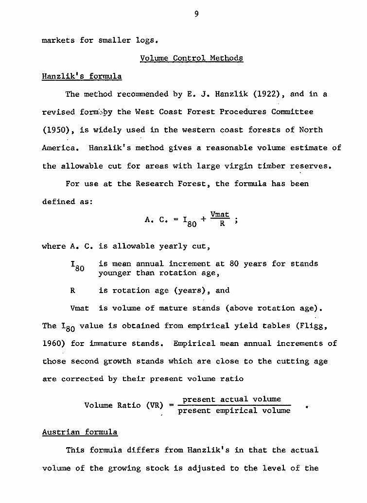
Hanzlik's formula
The method recommended by E. J. Hanzlik (1922), and in a
revised formbby the West Coast Forest Procedures Committee
(1950), i s widely used in the western coast forests of North
America. Hanzlik's method gives a reasonable volume estimate of
the allowable cut for areas with large virgin timber reserves.
For use at the Research Forest, the formula has been
defined as:
' 80 R *
where A. C. i s allowable yearly cut,
I i s mean annual increment at 80 years for stands younger than rotation age,
R is rotation age (years), and
Vmat i s volume of mature stands (above rotation age).
The IgQ value i s obtained from empirical yield tables (Fligg,
1960) for immature stands. Empirical mean annual increments of
those second growth stands which are close to the cutting age
are corrected by their present volume ratio
, , present actual volume Volume Ratio (VR) = — ~ : — =
present empirical volume
Austrian formula
This formula differs from Hanzlik's in that the actual
volume of the growing stock i s adjusted to the level of the
10
desired growing stock over the period of the rotation, whereas in
Hanzlik's formula the entire volume of old growth timber is
removed during the rotation. The increment used in the Austrian
formula is the mean annual increment of the entire stand at
present.
The formula i s : Ga - Gr A. C. = I + "
K
as presented by K. P. Davis (1954),
where A. C. i s allowable cut,
I i s mean annual increment during the conversion period,
Ga i s actual growing stock,
Gr i s desired growing stock, and
R i s rotation age in years.
In Heyer's formula, which is a modification of the Austrian,
the volume of the growing stock i s adjusted over a period which
is generally much shorter than the rotation.
Kemp1s formula
If volumes and areas by stand size classes are available,
this formula is easy to apply. It is used in properties on
which there is a surplus of timber beyond rotation age. The
objective in application i s to determine the cut that w i l l
achieve an approximately equal distribution of area by age or
tree size classes within a rotation with a minimum variation

11
from ultimate sustained yield volumes.
For a forest type the expression i s :
7A + 5A-, + 3A„ + Ao A. C. ~ (MA)
4R
(U.S. Dept. of A g r i c , 1958),
where A. C. is annual cut,
A is area of sawtimber stands,
A^ is area of poletimber stands,
A£ is area of seedling and sampling stands,
A-j i s non-stocked area,
R is rotation in years, and
MA is expected average volume per acre of stands as they are cut.
The formula simply represents the distribution of volumes
as they should be in a normal forest, i.e., in a triangular
diagram of the growing stock in a normal forest, the forest
should have:
1/16 of i t s volume in stands between 0 and 1/4 rotation age,
3/16 of i t s volume in stands between 1/4 and 1/2 " " ,
5/16 of i t s volume in stands between 1/2 and 3/4 " " ,
7/16 of i t s volume in stands between 3/4 and rotation age.
This model i t s e l f i s erroneous in that volume plots"over
age as a second or third degree curve instead of a straight line.
This error is comparatively minor, however, and applies to some
other allowable cut formulae as well" (U.S. Dept. of A g r i c , 1958).

12
Barnes' method (Barnes, 1951)
Since the annual cut i s closely related to the age at
which the stands are harvested, an estimate of the average
cutting age during the forest rotation should furnish a good
estimate of the annual cut. Therefore, in Barnes' method
the average present age must be calculated, to see whether
i t i s over or under the average age of a normal forest, with
an average cutting age equal to the rotation. For example,
in a normal forest with an average cutting age of 80 years,
the present average age should be 40 years, but i f the average
age of the forest i s more, or less, than 40 years, a discre
pancy w i l l occur, with which the average cutting age must
be corrected. The yield at this corrected average cutting
age w i l l give a reasonable estimate of the yearly cut accord
ing to the hypothesis.
Since empirical yield tables are available for Br i t i s h
Columbia, the average yield can be read directly from the
yield tables for different types. The weighted average of
these yields at the calculated rotation age then w i l l give
the allowable cut, based on Barnes' assumption.
Black H i l l s formula
This formula has been applied on the National Forests in
the Black H i l l s of South Dakota, as described by K. P. Davis

13
(1954). Two broad condition classes of merchantable timber are
recognized:
1. Mature stands, in which i t i s presumed current losses
equal increment.
2. Thrifty merchantable stands, making net increment.
The formula is as follows:
VM' (CM) + [vt + (It/2)] Ct A. C. = • -—; ;
where A. C. i s allowable cut,
VM is volume of mature stands,
CM is per cent cut in mature stands, an arbitrary figure, developed on the basis of s i l v i c u l t u r a l and related considerations,
Vt i s volume of th r i f t y merchantable stands,
It is increment of t h r i f t y merchantable stands during the cutting cycle,
Ct i s per cent cut in t h r i f t y merchantable stands (an arbitrary figure determined in the same way as for CM), and
Y i s cutting cycle in years.
Hundeshagen's formula
Hundeshagen1s assumption was that growth or yield in an
actual forest, approximately regular in distribution, bears the
same relation to i t s total growing stock as growth in a f u l l y
stocked regulated forest, as represented by normal yield tables,
bears to i t s growing stock (K. P. Davis, 1954). Expressed as a
proportion:

14
Ya = Yr . Ga = Gr '
where Ya is growth or yield in an actual forest,
Ga i s growing stock in an actual forest,
Yr is growth or yield in a f u l l y stocked forest, and
Gr is growing stock in a fu l l y stocked forest.
The f i n a l equation i s : Yr
Ya = — Ga . Gr
Yr
If the — ratio is expressed as a percentage a quick approxima
tion of the yield in the actual forest can be made by merely
multiplying this percentage by the actual growing stock. This
method, however, has many limitations regarding comparability of
data, such as standards of u t i l i z a t i o n , effect of understocking
and the l i k e , inherent to the direct application of normal yield
table data to actual stands. Although some of these factors can
be eliminated using empirical yie l d tables, the method s t i l l should
be used with caution and at best i s useful only for a rough
approx imat ion.
Von Mantel's formula
It has been observed that in an approximately f u l l y
regulated forest there i s a f a i r l y regular and often linear
increase in volume by age classes. This suggests the possibi
l i t y that the growing stock can be represented by a right
angled triangle. The area of this triangle therefore represents
the total growing stock of the forest, "Ga", having the base of

15
"R" acres, and the altitude, the yield at rotation age, "Ya",
indicating the annual cut. Thus the area of the triangle i s
given by the formula:
R(Ya) . iia =
hence the actual yield i s : 2Ga Ya - — .
The accuracy of the formula i s greatly affected by the
regularity of the forest. It is obviously inapplicable unless
there is some semblance of regularity.
Sven Petrini's (1956) compound and simple interest formulae
If the annual cut m i s to be calculated for a period of t
years, where the present wood capital i s k cu. f t . , the actual
percentage of increment i s £ per cent and the f i n a l capital of
wood is set as K cu. f t . at the end of t period; then m can be
calculated using the compound interest formula:
k(1.0p) t - K m " 0 * 0 p l.Opt - 1 •
If we assume that the capital k increases an equal annual
amount, then the actual annual percentage increment in rea l i t y
is continually diminishing during the period, which i s usual
for older stands. Thus the formula given below i s better
suited to stands with slow growth, while the equation above w i l l
more l i k e l y give a better answer for faster growing t h r i f t y stands,

16
The simple interest formula i s :
k ( l + TUTD - K m = tp
t ( l + 200 + tp)
In this formula i t i s assumed that the volume of the
fel l i n g s , when made continually each year, can be reckoned as
having been growing during half the period in question, i.e.,
t/2 years.
W. H. Meyer's amortization formula
This method, originally developed by W. H. Meyer in 1943,
has been modified and described by him in 1952. It i s almost
identical to Sven Petrini's compound interest formula, except that
Meyer includes ingrowth in his calculations, and therefore
obtains a higher allowable cut volume than Petrini.
Meyer's formula i s as follows:
v G ( i + g t ) m - v m
A. C. = gM 5 ;
where A. C. i s yearly allowable cut,
e i s compound growth rate for the merchantable stands alone excluding ingrowth,
V Q i s present volume,
V m is volume at the end of the period,
m is period for which the allowable cut is desired, and
gt is compound growth rate of the entire stand.
In comparing overall accuracy, the W. H. Meyer method can
be judged more accurate, because of his corrections regarding
17
ingrowth, than Petrini's formula.
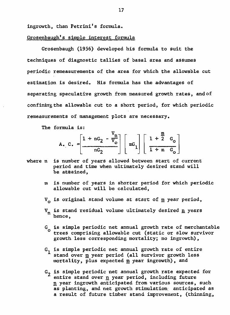
Grosenbaugh1s simple interest formula
Grosenbaugh (1956) developed his formula to suit the
techniques of diagnostic t a l l i e s of basal area and assumes
periodic remeasurements of the area for which the allowable cut
estimation i s desired. His formula has the advantages of
separating speculative growth from measured growth rates, and of
confining the allowable cut to a short period, for which periodic
remeasurements of management plots are necessary.
The formula i s :
A. C. -
Vn-1 + nG9 - w—
*• o nG 0
mG,
m 1 + 2 G,
1 + m G o J where n i s number of years allowed between start of current
period and time when ultimately desired stand w i l l be attained,
m i s number of years in shorter period for which periodic allowable cut w i l l be calculated,
V Q i s original stand volume at start of m year period,
V n i s stand residual volume ultimately desired n years hence,
G i s simple periodic net annual growth rate of merchantable trees comprising allowable cut (static or slow survivor growth less corresponding mortality; no ingrowth),
G.. i s simple periodic net annual growth rate of entire stand over m year period ( a l l survivor growth less mortality, plus expected m year ingrowth), and
G2 is simple periodic net annual growth rate expected for entire stand over n year period, including future n year ingrowth anticipated from various sources, such as planting, and net growth stimulation; anticipated as a result of future timber stand improvement, (thinning,

18
salvage, and removal of slower-growing items).
H. A. Meyer method (Meyer. Recknagel. Stevenson. 1952)
This i s a time-consuming method to apply when detailed
data are available. Originally i t was designed for all-aged
stands but i t is applicable to even-aged stands as well. The
method involves the calculation of the average number of trees
by diameter classes, average volume per tree, average volume
per acre, and decadal growth rates for the total area, including
a l l species. The number of trees per acre and volume per
acre values must be weighted by the appropriate areas to
obtain the correct average values. The decadal growth rates
are not weighted. When a l l these data are available, then a
regression equation i s calculated, using the logarithm of
the number of trees per acre in each diameter class, and de
Liocourt's quotient i s evaluated, using the equation:
-D
N = k q T
where N i s number of trees per acre,
k is constant,
D is diameter at breast height (inch), and
i i s diameter class interval (inch) (Sammi, 1961).
The k i s calculated from the equation by inserting D = 0 in the
exponent. Thus the equation becomes: N = k. Substituting this
k value together with an N and a D value calculated from the

19
regression equation, £ can be easily obtained as:
Knowing £ and the average growth rates of the diameter
classes, the per cent volume increase can be read from a table
presented by Meyer, Recknagel and Stevenson (1952, p.159).
Multiplying the per cent volume increase by the average volume
per acre values, the volume increase by diameter classes can
be obtained. By subtracting the average mortality rates from
the corresponding volume increase figures and summing up these
reduced values, a net volume increase for the total forest can
be shown in a table form, similar to Table 33 in Meyer, Recknagel
and Stevenson (1952).
Usually when determining the allowable cut, a reduced £
is used and a maximum diameter limit is set, beyond which a l l
trees are cut in a certain period of time.
Generally the £ i s compared to the £ of well-managed Swiss
forests and reduced accordingly. However, i f the present £ i s
lower than that of the Swiss forests, reduction may not become
necessary.
Area and Volume Control Methods
Area-volume computation
The formulae described above usually give only a guide con
cerning the quantity of the yearly allowable cut. The West
Coast Forest Procedure Committee (1950) recommended that a l l

20
formula methods should be followed by an area-volume check,
described in detail in the report. This check requires knowledge
of the areas, stocking, site, and species composition by age
classes. If empirical yie l d tables are used " as in this case -
stocking data are not essential.
The procedure begins with the statement of the areas, and
the statement of a t r i a l allowable cut figure obtained by one
of the methods described previously.
When different type groups are present i t i s necessary to
reduce the areas to a basic type as when area regulation is used.
The next step i s to obtain a preliminary estimate of the
duration of cut, by dividing the area of the f i r s t type or age
group by the yearly cutting area. Half of this duration age
then i s added to the age of the stand when cutting begins, thus
obtaining a preliminary estimate of the average cutting age.
For this average cutting age the corresponding yield i s read
from the empirical yield table, and multiplied by the actual
number of acres, thus obtaining the total cut in that type.
This volume then i s divided by the preliminary allowable cut
estimate, to see how many years the volume would last in that
particular type. This period usually does not coincide with
that estimated previously, using the yearly cutting area, and
therefore half of the revised duration period must be added to
the age of the stand when cutting begins, to obtain a new
revised average cutting age.

21
A new yield per acre based on the revised average cutting
age, and multiplied by the actual acres in the type, w i l l give
the actual revised yield for the whole type when cut. The
f i n a l two columns show the duration of the cut per type and
cumulative times, assuming that the indicated allowable cut
volume w i l l be cut each year.
The next age group or type naturally w i l l have an age,
when cutting begins in i t , equal to the sum of i t s present
age and the figure shown in the cumulative column.
Otherwise a l l calculations are the same for this type as
have been described for the previous type. At the end of the
calculation the f i n a l cumulative column must coincide with the
rotation age, or must be at least within 5 per cent of the rota
tion to j u s t i f y the indicated cutting rate (The Westn. For. and +
Cons. Assn., 1950). If the difference is more than - 5 per cent
of the rotation age, the process must be repeated with a higher
or lower allowable cut volume, u n t i l the calculated rotation age
is within the required l i m i t . . This figure of allowable cut i s
used only for the f i r s t decade and then the allowable cut is again
determined on a basis of data then available.
Naturally this method is highly dependent on the yields per
acre read from the empirical yield tables. This can give an
erroneous estimate 70 or 80 years hence, particularly for pre
sently immature or recently-planted areas.

22
Combined method of allotment
This method, as described by Professor Z. Fekete (1950),
intends to combine the advantages of the area regulation and the
volume regulation in such a way that the yields on nearly similar
cutting areas w i l l become close to equal.
In a forest where the distribution of the age classes is
f a i r l y even, area regulation and volume regulation give almost
the same answer. But, where the age class distribution is
irregular, the area regulation might indicate irregular yields,
while the volume regulatory methods might indicate irregular
cutting areas.
In this case the combined method of allotment may be used.
This lessens the irregularity of the yields obtained by the
area method and at the same time reduces the differences between
the periodic cutting areas.
The combined method starts out from the area regulation
with the simplification that the yields are shown only in the
f i r s t and second cycle. These yields are equalized (averaged)
and corresponding areas calculated.
The cuttings of the f i r s t cycle proceed according to this
plan. Before the beginning of the cuttings in the second cycle
another cutting plan must be prepared, equalizing the yields of
the second and third cutting cycles. A l l the other cutting
plans are prepared the same way.

23
The combined method gives a more even periodic yield than
the yields obtained by area regulation, and the differences
between the periodic cutting areas w i l l also be less than
those obtained by volume regulation.
This method reduces the disadvantages of the two methods
just mentioned and is a simpler process. Therefore i t became a
popular regulatory method in central European practice.
The area-volume method calculates with periodic cutting
volumes, giving room for some variation in the yearly cuts.
It uses volumes available for cut in the immediate future
(within two cutting cycles), and reduces the possibility of
making undetectable errors for future stand-volume conditions.

24
NECESSARY INFORMATION
For t r i a l of the widely different allowable cut calcula
tion methods, a wide variety of data was needed.
In the case of the University Research Forest, much informa
tion was available, but this was inadequate because i t was in
various units of measurement, and taken at different times.
Therefore i t was decided to undertake a small scale survey to
obtain the data in one uniform measurement of wood (cu. ft.) and
in such a way that a l l the necessary information for the formulae
and methods mentioned previously could be evaluated.
The headings of the cruise sheets had to be planned to
include necessary stand information, and classification standards.
After considering many p o s s i b i l i t i e s , i t was decided that a
combined method of photo- and ground-cruising would be employed,
using the up-to-date photographs of the Research Forest and the
point-sampling method, devised by B i t t e r l i c h in 1948 and
further developed by Grosenbaugh (1952, 1955, 1958).

25
DATA COLLECTION AND CALCULATION METHODS
Classification
Before ground sampling could begin the stratification of
forest types had to be completed to provide a good base for
the distribution of sample plots. Therefore classification
limits were set up and a l l forest types were sorted into these
classes.
The following age classes were established:
Age Classes Limits (years)
Old Growth (O.G.) 160 +
Second Growth (S.G.) 30 - 159
Young Growth (Y.G.) 1 0 - 2 9
Planted (PL.) 0 - 9
Forest types
Types were determined according to the order of predominance
in the crown closure or volume of a species depending on whether
the type was just estimated from photographs or was also visited
and sampled on the ground.
A l i s t of a l l tree species found on the University Forest was
given by the U.B.C. Forest Committee (1959). However, in this
work only Douglas f i r (Pseudotsuga menziesii var. menziesii (Mirb.)
Franco), western hemlock (Tsuga heterophylla (Raf.) Sarg.), and
western red cedar (Thuja plicata Donn) volumes were considered.

26
The present study showed that these three species comprise
approximately 98 per cent of the total volume in the Research
Forest.
To f a c i l i t a t e the later use of empirical yield tables the
same type groups were selected as they are shown in the empirical
yield tables in Zone 2 (Fligg, 1960), from which the following
types were recognized:
Douglas f i r types (Growthttype 2),
Cedar types (Growth type 5),
Hemlock types (Growth type 7).
Site classes
Similarly to the forest type classification, the chosen
site class limits were identical to those established in Fligg 1s
(1960) Empirical Yield Tables (p.11), separating good G, medium
M, poor P and low L sites for different types, and showing the
site index limits based on heights at 100 years of age.
Diameter classes
Two-inch diameter classes were chosen, because in most cases
this proves satisfactory for management purposes, and eliminates
a great deal of extra work.
It is necessary to mention that the estimates made from the
photographs or taken on the ground were measured and recorded
as accurately as possible, though later they were sorted into
the classes described above.

27
The Use of Aerial Photographs
Photo typing
The photographs used were black-and-white, semi-matte in
finish, 9 x 9 inches in size, had a representative fraction (R.F.)
of 1:15,900, and were taken in June, 1961.
The minimum area in any type was five acres. Types were
separated with a black b a l l point pen using a pocket stereoscope
on the basis of the previously stated classification standards.
Ages were not directly estimated from the photographs, but
were taken from an age map prepared from previous forest cruises
of the area.
The forest types (species composition) were directly e s t i
mated from the photographs, using existing forest cover maps as
a reference in doubtful cases.
Stand site indices were obtained from two separate estima
tions, namely: from the age estimation and photographic height
measurements.
The latter were carried out for each individual type,
measuring the height of one or two trees, representing the ave
rage maximum height of the stand (roughly average height of domi
nant and codominant trees). The site index then was taken from
the appropriate B.C. Forest Service site index curves (Fligg, 1960).
Photographic height measurements
Photographic height measurements of trees were carried out
using an Abrams height finder and the most commonly used parallax

28
formula: H dp
h = P + dp
where h i s height of the tree in feet,
H i s flying height above ground in feet,
dp i s parallax difference read from the height finder (mm),
P i s base length as measured from photographs (mm,).
To speed up measurement a combined graphical solution of '
the parallax formula was used which corrected the errors re
sulting from the tree's being on an elevation different than the
average height of the two principal points:
F i r s t , basic lines were calculated for each different P
value measured from the photographs from which the equivalent
height in feet for one mm. parallax difference could be read.
The equation of these lines was:
0.01 h p = H P + 0.01
where hp i s height in feet at elevation of average value of the principal points ( f t . ) ,
H i s flying height ( f t . ) , and
P is average length of the principal points (mm.).
The calculation was carried out only for two different
flying heights, because the equation above indicates a straight
line, for which two points are adequate.
The next step was to construct the correction lines by cal
culating the parallax differences, which occur when trees are

29
higher or lower than average elevation of the principal points.
For this purpose the equation used was:
H - h
where dp is parallax difference between the base of the tree
and the average height of the two principal points (mm.),
P i s average base length between principal points (mm.),
H i s average height of the two principal points ( f t . ) , and h i s elevation difference between the average height of
the principal points and the base of the tree (mm.).
When different values of h were substituted in the equation
a slightly curved line resulted.
These correction lines were plotted on the same graph,
showing the height corrections in feet for differences in
elevation.
To obtain a tree height the steps outlined below were
followed:
1. Calculate average base length of the stereo pair.
2. Calculate average flying height above principal points.
3. Obtain elevation of the tree base.
4. Measure parallax difference of tree.
5. Find average flying height H on the x axis of the graph.
From that point go perpendicular u n t i l the line of the
average base length is met. (From this point the
correction lines must be followed paral l e l , u n t i l the
corresponding vertical line marking the elevation of

30
Graphical solution of the parallax formula Figure 3
/ Elevation above sea level (ft) 2000 1500 1000 500
140 145 150 155 159 Flying height above ground (100 ft)

31
the tree base is hit.) At this point the correct value
of the 0.01 mm. parallax can be read from the y_ axis.
For example, P = 89.65 mm., H = 14,640 f t . , elevation
of the tree base 1,000 f t . , then the 0.01 mm. parallax
difference corresponds to 1.690 f t . on the ground.
Multiplying the value read from the y axis by the
total parallax difference read from the height finder
gives the total height of the tree (Figure 3).
Area determination
Although the total area of the Forest was known (9,774 a c ) ,
a detailed area determination was necessary for each individual
type, to furnish the base for stand-table projection, and
for the allocation of future cutting areas.
It was decided to usethe grid area-determination system
described in Spurr (1960), combined with a correction method
suitable for mountainous areas.
The calculation of the number of points necessary to give
a desired accuracy was given by Spurr (1960).
M i - P) (t2) N - E P
2 - - • ;
where N is number of points necessary,
P i s per cent of class limit of the total area,
Ep is error per cent of class limit, and
t is s t a t i s t i c a l constant.

32
Using the values of the 5 acre class limit:
P = 5 x 100 = 0.0512, 9774
Ep = 0.009, and t = 1.96,
N = = 2,351 points at sea level.
The distance in inches of these points on the photograph
when distributed evenly i s :
Rounding this distance to 0.300 inches and recalculating Ep and
N, we obtain 0.0083 per cent and 2,694 points respectively.
Since the photographs were taken over mountainous terrain,
i t was necessary to weight the areas represented by these points
by elevation. For example, because of scale differences, a point
appearing at 2,000 feet elevation w i l l represent a much smaller
area than one appearing on sea level, assuming the spacing of
these points is even.
Reduction factors were calculated using the equation:
Dp = 12
= 0.321 inches. 15,900
EL W = (1 - 15,900
where W i s weight of the plot, and
EL is elevation in feet.

33
TABLE 1
WEIGHTS OF POINTS BY ELEVATION LIMITS
Elevation Limits (ft.) Weights
0 - 200 0.9875 201 - 600 0.951 601 - 1,000 0.902
1,001 - 1,400 0.855 1,401 - 1,800 0.809 1,801 - 2,200 0.764 2,201 - 2,600 0.721
The evenly-spaced points were pricked on the photographs
and a transparent overlay was prepared showing the elevation
limits.
Counting the number of points f a l l i n g into a type multi
plied by the corresponding weight gave the number of points
which would have fallen into that type i f i t were at sea level.
The influence of sloping terrain became evident when the
fi n a l total reduced number of points was counted and compared to
the calculated number of points at sea level. A discrepancy of
-3.12 per cent of the total area resulted and had to be d i s t r i
buted proportionally to the individual types. This underestimate
is due to the steep sloping terrain on many parts of the Research
Forest, especially the so-called " P i t t Lake slope". (Corrected
areas are shown in Tables 3 and 6.)
A brief comparison of the areas shown in 1958 to the present
condition was based on the data published by the University
Forest Committee (1959).

34
TABLE 2
COMPARISON OF AREAS AS ESTIMATED IN 1958 AND IN 1961.
Difference Class 1958 (ac.) 1961 (ac.) based on 1958 (ac.)
Productive land Road Rock
9,100 80
180 313 90 11
9,282 48 30
340 57 17
- 32 - 150
182
Swamp Urban
Water 27 - 33
6 TOTAL 9,774 9,774
Considerable differences between the two area estimates are
present. The reason of these discrepancies can be explained
mainly by the actual changes in the areas (e.g. urban) and
partly by the sampling approach of the point-grid area-estimation
method. However, other facts which may cause large differences
between the two estimates must also be mentioned. In the present
method, some of the areas which were classifi e d as rock and
poor and rocky on the Abernethy and Lougheed (AV&L.) part of the
forest were classified as poor stocking and l i s t e d in the
productive land area. Also, i t should not be forgotten that
since 1958 the vegetation might have covered a large part of
these small rocky areas, therefore many of these small rock
outcrops may have appeared on the 1961 photos as productive
sites.

35
TABLE 3
AREA SUMMARY FOR THE UNIVERSITY RESEARCH FOREST
East Side West Side Total Forest (Y.G.) * (O.G.. S.G.) *
TYPE AREA (ACRES)
Stocked 3,793 5,489 9,282 Road 29 19 48 Rock 7 23 30 Water 46 294 340 Swamp 42 15 57 Urban 17 17 TOTAL 3,917 5,857 9,774
* Y.G. stands average 25j years in age; S.G. stands average 80 years, and O.G. stands are more than 300 years old.
The differences in the water and swamp classes may be due to
the season when the measurements were made. Hence, in one case,
swamps could have been classifi e d as water, while in a drier
part of the year they obviously appear as swamps, and could
have been sorted into the swamp class. Note that only 6 acres
difference appears between the sum of water and swamp classes
between the two measurements (1958 and 1961).
Another comparison of the areas in the productive class
is shown below:

36
TABLE 4
COMPARISON OF PRODUCTIVE AREAS AS ESTIMATED IN 1958 AND IN 1961
Type 1958 (ac.) 1961 (ac.) Difference from 1958 (ac.)
O.G. 916 994 + 78 S.G. and scattered O.G. 3,162 3,701 + 539 Y.G. P. 3,340 3,676 + 336 Planted and cultivated 440 558 + 118 Hardwood and scrub 1,242 353 - 889
TOTAL 9,100 9,282 About 250 acres of old growth (O.G)) were logged 1958-1961.
The largest discrepancy is in the scrub type, and is caused
by the extreme overestimation of scrubby areas in 1958, on the
P i t t Lake slope and on the A.&L. part of the Forest.
The recent estimates, however, show that no such large
acreage of scrub exists on these areas. On the P i t t Lake slope
there are mostly well growing, satisfactorily stocked stands of
low site quality, leaving just a small area for scrub and
several stands of alder and maple.
No definite evaluation has been made regarding productive
stands of the A.&L. part of the Forest, since only the areas of
the following classes were estimated by the writer:
Total area, Stocked, Road, Rock, Water, and Swamps.
Detailed area estimates of the stocked classes in the A.&L.
part of the Forest as shown by Bajzak (1960), were proportionally
distributed to the recent estimate of the stocked area.

37
The Use of McBee Punch Cards
The individual measurements of the types were recorded on
McBee punch cards for easier selection. The card was divided
into columns where the number of the type, estimated crown
closure, species composition, etc. were recorded.
The actual order of numbers and headings on a McBee card
appeared as follows:
Photo Type Crown Species Date Height His- Area S.I. S.I. number number clo- compo- of tory code
sure sition establishment
The descriptions of the items are as follows:
Photo number: Gives the number of photograph on which the type represented by a type number (second column) appears.
Crown closure: Is a number which shows the area covered by the crowns in relation to the total area, in 10 per cent units.
Species composition symbols are similar to those appearing in the empirical yield tables.
Date of establishment marks the century and decade in which the stand was regenerated. For example, a stand regenerated in 1860 w i l l have a date of establishment "86".
Height of the stand in feet appears as i t was measured on the photographs.
History: A sign indicates the cause responsible for re-establishment. Thus © designates clear cutting,
0 designates f i r e , and ^ designates selective
cutting. The combination of these signs can also appear.

38
Area of the type is shown in acres.
Site index is shown as taken from the corresponding B.C. Forest Service site index curves. For example, in a type having a species composition of FH (Douglas fir-hemlock), the site index appearing was taken from the Douglas f i r site index curve, but where HC (hemlock-cedar) or CH type was present, the site index was taken from the HC site index curve.
Site indices taken from the various site index curves
were not considered adequate for some calculations. Therefore
a site index code was established for reducing site indices to
the same level. This was done using the B.C. Forest Service
Site Index curves, which show that the limits of the site index
classes are higher by 10 feet for Douglas f i r , than for hemlock
and cedar. Thus:
The site index code for Douglas f i r types = (S.I. - 20) 0.025
The site index code for hemlock and cedar
types = (S.I. - 10) 0.025.
After the substitution of the various site indices into the
appropriate equation above, the calculated code gave the equiva
lent ranges of the site classes in the same units. Thus the site
indices regardless of species became equivalent to the codes
shown as follows:

39
TABLE 5
SITE INDICES AND CORRESPONDING CODES
Site classes S.I. Limits (ft.)
Douglas f i r Hemlock and Cedar Codes
Low 0 - 6 0 0 - 5 0 0 - 1.0
Medium Poor
Good
61 - 100 101 - 140 141 +
51 - 90 91 - 130
131 +
1.1 -2.1 -3.1 +
2.0 3.0
Example: If a medium site land bearing a Douglas f i r stand
shows a site index of 130, the same land, bearing a hemlock stand,
would show only a 120 site index. Using a code, both stands
less of species. Naturally the codes can be easily reversed to
either Douglas f i r or hemlock site index values, by rearranging
the equations above. These values were then available for use
with the empirical yield tables and for converting cover types
to the FH medium site standard. Also, using these reduced
values, the calculations of the weighted average site index for
the types and for the whole of the Forest were easily carried
out, by converting the average codes to Douglas f i r site index
values.
The summary of the average ages and site indices is shown
in Table 6.
would have a 2.75 code, indicating a medium site quality regard

TABLE 6
AREAS, SITE INDICES, AVERAGE AGES, GROSS CU. FT. VOLUMES BY MINIMUM DIAMETER CLASSES, AND SPECIES COMPOSITIONS BY AGE AND SITE CLASSES
* Class O.G.G. O.G.M. O.G.P. AREA (ac.) 159 671 164 S.I. (F) (ft.) 161 117 76 AVG. AGE (yrs.) 230 260 240
• • 3.1 2,197,062 9,200,752 1,587,028 GROSS * -5 VOLUME W . w
9.1 11.1
2,161,923 2,145,387
8,928,997 8,852,503
1,483,544 1,406,792
Q (CU.FT.) . H
55 S 13.1 2,136,006 8,694,818 1,296,092 Q
(CU.FT.) . H 55 S a
Species Composition HF CH CH
Class S.G.L. Y.G.G. Y.G.M. AREA (ac.) 43 2170 1171 S.I. (F) (ft.) 50 135 125 AVG. AGE (yrs.) 90 30 25
• / • — » 3.1 208,034 2,444,288 238,685 GROSS w* ̂ 9.1 968,666 49,861 VOLUME Q ^ 11.1 561,856 19,333 (CU. FT.) g ' g
M M 13.1 304,429 11,452
Species Composition FH HC HC
S.G.G. 805 161 70
7,430,150 6,802,250 6,206,550 5,535,180
FH
Y.G.P. 335 85 20
5,236 12,737 3,645
S.G.M._ . S.G.P. 1885 121 80
20,587,970 17,984,785 10,599,310 14,446,640
FH
PL. 558 134 5
968 83 90
6,578,528 3,554,496 2,269,960 1,466,520
HF
HW. 353 113 40
CH Abbreviations of classes are explained on pages 44 and 45.

41
Ground Sampling
It was decided that probability (point) sampling techniques
would be used for determination of the number of trees per acre,
diameter growth, and bark thickness values in different types.
Only 98 point samples were distributed to the different
strata. In addition to these, the existing permanent sample
points and temporary plots from the A.&L. part of the Research
Forest (Bajzak, 1960) were used to furnish the required data for
the stand table projection purposes.
The numbers of those types sampled were selected using a
random number table. The sample centre points were located
measuring f u l l chain lengths from a clearly distinguishable point
v i s i b l e on the photograph, f a l l i n g in or close to the type. The
bias from personal judgement was thus eliminated, and reasonable
randomness in the location of the sample points was achieved.
For the determination of trees f a l l i n g into the sample, and
tree height measurements, the Austrian-made Spiegel relascope was
used. It was found to be a very convenient, accurate and handy
instrument, although the optical distance measurement in old
growth stands was not very practical.
For checking "border trees", Stage's (1959) cruising
computer was used, which was also found convenient for the rapid
calculation of tree heights.
The role of the Spiegel relascope in the sampling was

42
simply to determine the trees which had to be measured. Then
the diameter of the selected trees was measured with a diameter
tape, and recorded to the nearest tenth of an inch. A l l trees
larger than 3.0 inches at breast height were measured.
For age, diameter growth, and bark thickness determina
tions, increment borers were used. Every fourth tree in the
plot was bored. Measurements were recorded to the nearest
hundredth of an inch, for both the increment core lengths and
bark thicknesses.
Decayed, or partly-living boles (as was common on cedars)
were not bored.
The following headings were used on the t a l l y sheet:
Type No.: B.A. Factor: Date:
Spec. D.B.H. Cond. Crown Double 10 yrs. 20 yrs. Age at Height class class bark growth growth B.H.
thickness
Species symbols used in the inventory are l i s t e d below:
Symbol Species
F Douglas f i r H Western hemlock, or hemlock C Western red cedar, or cedar Cy Yellow cedar B Abies species D Red alder PI Lodgepole pine Pw White pine

43
Under the heading of condition class (cond.class) the
following were recorded:
1 l i v i n g tree,
2 a dead tree (died within the last five years).
Trees that died before 1956 were not included in the cruising.
Four different crown classes were also distinguished as:
1 dominant,
2 codominant,
3 intermediate,
4 suppressed.
Heights (Ht.) were measured to the nearest foot.
It may be of interest to note the r e l i a b i l i t y of photo e s t i
mates and compare them with the results obtained by the ground
measurements.
Species composition estimates were correctly recorded
(f a l l i n g within the same type group) 88 per cent of the time,
while age class determinations were 91 per cent correct in compari
son with the ground checked types. Height measurements, however,
in most cases showed a great variation on the photographs as
well as on the ground. Naturally, ground estimates, in a stand
with widely variable heights, taken from an inadequate number of
samples, cannot be considered as a sufficient base for comparison.
Photo estimates of average stand heights in this situation should
provide a more reliable, but slightly conservative, source of
information for stand site index calculation purposes.

44
In this particular case, after ground checking, the measure
ments taken from the aerial photographs were corrected and used
for site index determination.
Calculations
Having finished the photo and ground sampling, the necessary
calculations for the stand table projection process had to be
carried out. The method of the stand table projection was that
described in detail by W. H. Meyer (1952). The required data
are:
Number of trees per acre,
Mortality ratios, and
Periodic diameter growth by diameter classes.
The stand table projections were carried out only for the
main species, namely, Douglas f i r , hemlock, and cedar.
Method of Calculating the Number of Trees per Acre.
and Mortality Rates
Because some of the allowable cut methods required separate
data by age, site, and condition classes, i t became necessary to
select trees by species for the following age and site classes:
Old growth, good site (O.G.G.)
Old growth, medium site (O.G.M.̂
Old growth, poor site (O.G.P.)
Second growth, good site (S.G.G.)
Second growth, medium site (S.G.M.)
Second growth, poor site (S.G.P.)

45
Second growth, low site (S.G.L.)
Planted (PL.)
Hardwood (HW.)
Although in the young growth (Y.G.) stands the data given by
Bajzak (1960) were not similar to the site classes required for
this work, his good, medium and poor stocking classes could be
f i t t e d into the present site classification. His nomenclature
has been kept, but i t should be noted that i t means stocking
classes here, and not site classes.
Young growth, good (Y.G.G.)
Young growth, medium (Y.G.M.)
Young growth, poor (Y.G.P.)
Prior to computer calculations on the Alwac III-E a l l data
for the computation of the number of trees and for further
sorting had to be transferred to numerical symbols.
Species codes F i r (1), H (2), C (3) , diameter at breast
height in inches, codes defining whether the tree was alive (1),
or had died within the last five years (2), and the horizontal
point factor (H.P.F.) which is equal to 183.346 times basal area
factor (Grosenbaugh, 1958, p.16), were typed, starting with the
species code in each line.
Simultaneously, these data were automatically punched on a
tape to make the data readable for the machine. When calculating,
the computer took in a row of data and executed the following

46
equation:
D Z
where N i s number of trees per acre,
H.P.F. is horizontal point factor, and
D is diameter at breast height.
The theoretical base of these calculations i s inherent to
the point sampling theory:
"It must be remembered that point-sampled trees are not
sampled proportionally to their frequency as plot-sampling
would do. Hence, their basal areas, volumes, frequency, etc.
should not be given the same equal weight as in plot-sampling.
Instead, before any further calculations are made, each point-
sampled tree should have i t s basal area, volume, frequency, etc.
weighted inversely as i t s probability of being sampled.
Dividing each sample-tree basal area, volume or frequency by
i t s own basal area does this." (Grosenbaugh, 1955, p.19.)
Finally, "blow up" factors or multipliers are needed to
convert point sample ratios to a per acre basis. The horizontal
point factor (H.P.F.) assumes that the denominators of the ratios
w i l l be tree diameters in square inches. (This constant i s
called basal area factor, when denominators of the ratios are
tree basal areas in square feet.)
After computer calculation of the number-of-trees-per-acre
value, the sorting of the different tree species into 2-inch
47
diameter classes was carried out. The summation of the number-
of-trees-per-acre values f a l l i n g into the same diameter class
within a type group was done by hand, as well as other calcula
tions after this point.
To obtain the f i n a l value of the number of trees in a
diameter class for an age and site class, the sum obtained this
way had to be divided by the number of point samples f a l l i n g
into that type group. In a similar way the number of trees per
acre that died within the last five years was calculated.
These latter values had to be multiplied by two, to obtain ten-
year mortality. From these two number-of-trees-per-acre values,
mortality ratios were easy to get, by dividing the number of
dead trees per acre by the number of li v i n g trees per acre.
These values appear in Tables 8, 9 and 10.
Some indication of the v a r i a b i l i t y of the mortality e s t i
mates can be given by showing the minimum and maximum estimates
of number-of-trees-per-acre mortality during the past decade,
in the various forest type classes.
For Douglas f i r , hemlock and cedar species, mortality
ranges per acre by forest type classes are presented as follows:

48
TABLE 7
MINIMUM AND MAXIMUM NUMBER OF DEAD TREES PER ACRE
BY SPECIES AND TYPE CLASSES
Type No. of dead trees per acre Number • of Minimum Maximum plots or sample
F H C F H C points
O.G.G. 0 0 0 3.87 216.51 65.19 14 O.G.M. 0 0 0 4.61 482.17 358.10 33 O.G.P. 0 0 0 0 255.52 40.63 13 *S.G.G. 2.3 3.1 6.8 28.2 87.50 62.50 5 *S.G.M. 0 2.3 0 61.50 84.10 50.00 15 *S.G.P. 2.1 50.0 2.5 30.00 87.50 17.50 3 Y.G.G. 0 0 0 0 126.88 0 100 Y.G.M. 0 0 0 0 83.86 0 96 Y.G.P. 0 0 0 0 0 0 72
* Data taken from permanent sample plots.
The values clearly indicate that hemlock has the largest
mortality range among the species considered. In the old growth
stands this mortality was concentrated on the smaller diameter
trees (approximately 0 - 1 6 inches). The mortality of the
Douglas f i r was low in a l l stands.
It must be noted that in the second growth stands, as well
as in the young growth stands, about 80 per cent of the existing
white pines died within the last five years, and the few
remaining l i v i n g trees appear to be unhealthy or dying.

49
TABLE 8
NUMBER OF TREES PER ACRE (NT) AND 10-YEAR MORTALITY RATES (MR) BY AGE AND SITE CLASSES FOR DOUGLAS FIR
D.BoH. in .
OoG.G, NT MR
OoG.M. NT MR
O.G.P. NT MR
S.G .G. S oG0 Mo S.G.P. S *G .L. Y<> G «G. Y.G.M. NT MR NT MR NT MR NT MR NT MR NT MR
0.47 895.28 7.11 7.05 6027 0.45 8o05 0.23 231045 5o24 5.00
13.16 0.56 3.18 0.17 10o35 0.11 162o14 3.09 0.79 0.01 10o22 0.06 16.03 0.04 - 2.55 1.05
11.20 0.21 3.99 0.03 4o59 - 2.01 0.26 2052 0.01 10.09 0.02 11.07 - 0.81 0.26 2o81 - 14.56 0.04 = - 0.13 5o39 0.20 5o82 - 2.08 - 0.13 1.06 - 2.51 - 1.77 - 0.13 8.35 - 1.27 0.84 - 3.96 1.29 - 0o60 lo20 2.05 - 0.22 1.37 - 0.20 1.53 0.35 0.33 0o84 - 0.13 - - 0.12
Y.G.P. NT MR
4 6 8 10 12 14 1.26 -16 18 20 1.92 0?53 22 24 0.47 26 0.41 0.48 28 0c62 0.29 30 1.16 0.28 0,51 32 IcOl 0.22 34 1.36 0.39 36 0„62 0.17 38 0.19 -40 1.94 0.41 42 0.95 44 0.40 0.28 46 0.31 0.11 48 0.18 0.05 50 0.31 0.05 52 0.15 0.04 54 0.09 -56 0.10 0.04 58 0.27 0.10 60 0.33 62 0.07 64 0.20 66 0.18 68 70 0.10 0.05 72 74 0.05 76 78 90
0.14
0.91 0.75
0.52 0.81 0.38 0.92
0.23
0.15
4.17 2.92 2.08 0.42 0.42
0.09
0.07 0.07 0.06

50
TABLE 9
NUMBER OF TREES PER ACRE (NT) AND 10-YEAR MORTALITY RATES (MR) BY AGE AND SITE CLASSES FOR WESTERN HEMLOCK
DoB .Ho OoG o G. O.G. Mo O.G S. G o G. S .G o M. S.G «P p S.GoL. Y.G.G. in. NT MR NT MR NT MR NT MR NT MR NT MR NT MR NT MR 4 6.69 1.00 64.80 0.31 172.02 0.10 0.62 61.23 0.34 196.50 0.39 63.80 0.07 6 18.29 - 26.60 0.14 17.38 - 12.32 0.20 57.45 0.13 117.25 0.22 30.10 0.14 8 3.99 - 14.54 - 13.05 - 30.06 0.30 22.24 0.04 79.04 0.07 14.27 10 5.14 - . 5.70 - 21.32 0.12 17.72 0.08 16.00 - 37.60 0.01 6.58 0.12 12 2«13 1.00 6.36 0.10 5.92 0.34 10.74 - 27.16 - 18.71 0.17 1.88 14 6.82 0.37 5.43 - 5.52 0.55 5.84 - 12.79 - 9.08 - 0.81 16 6o50 - 3.31 - 9.17 - 3o58 - 6.51 - 2.35 - 0.26 18 4o81 - 4.05 - 6o07 0.14 - - 3.21 - - - 0ol3 20 2,66 - 1.91 - 3o91 - - - 2.93 22 1.66 - 3.48 0.07 2o36 0.23 - - 0.40 24 0.24 - 3.22 - 0o92 - 0.76 - 0.71 26 0.22 - 2.27 0.07 0.82 - 1.68 - - - 0o49 28 1055 0.10 1.81 - 1.42 - 0.29 - - - 0.43 30 0.58 - 0.84 - 0o61 - 0.26 32 0.27 - 1.40 0.07 0.28 34 1.16 - 0.58 0.47 0.73 36 0.51 - 0.43 0.42 38 0.47 - 0.38 0.21 40 0.67 - 0.21 - 0.17 - - - 0.12 42 0.61 - 0.19 44 0.54 - 0.35 46 0.13 - 0.11 48 0.34 - - - 0.12
Y.G.Mo NT MR
Y»G. P. NT MR
21.85 3.03 2.46
0.02 0.06
11.67 4ol7 0.42
0.05 0.09

51
TABLE 10
NUMBER OF TREES PER ACRE (NT) AND 10-YEAR MORTALITY RATES (MR) BY AGE AND SITE CLASSES FOR WESTERN RED CEDAR
DTB?H 0 O.G. G. O.G. Mo O.G. p. S o G o G. S 0Go M. S • G. P o SoG.Lo Y 0' NT MR NT MR NT MR NT MR NT MR NT MR NT MR NT
4 14.51 - = - 110.40 0.17 146.77 0.19 241.70 - 56.40 6 5.35 - - - 5.92 - 25.33 0o28 56.59 0.09 57.29 0.31 21o90 8 - 1.00 10.11 - 20.95 - 14.71 0.21 19.26 0.02 49.50 7.11 10 1.35 - 1.31 0.27 8014 0.38 27.01 - 13.33 0.02 23.68 2.95 12 - - 2.78 - 23.87 0.17 7.90 - 7.30 - 9.33 0.94 14 1.50 - 5.50 - 10.31 - 2.33 - 3.93 - 2.51 0.40 16 1.81 - 2.65 0.31 15.15 - 3.74 - 5.72 - 1.17 0.27 18 - - 5.08 0.14 7.56 - 3.05 - 5.45 20 - - 2.79 - 11.26 - 0.57 - 1.65 - 0.89 22 1.43 0.36 2.26 - 5.26 - 0.92 - 2.07 - 0.66 24 0.23 - 2.16 - 2.46 - - - 1.05 - 0.59 26 1.53 0.13 3.55 - 2.47 - - - 0.63 28 0.18 - 4.65 - - 1.00 - - 0.52 30 0o28 0.54 2.47 - 1.25 - - - 0.78 32 0.13 - 3.31 0.03 0.28 34 0.78 - 2013 - 0.73 - - - 0.18 36 0.60 - 1.89 - 0.22 - - - 0.15 38 0.81 - 1.00 • - 0.19 - - - 0.15 40 0.67 - 1.26 - - - - - 0.12 42 0.51 - 0.85 - - - - - 0.12 44 0.28 - 0.36 - - - - - - 0.11 46 0.55 - 0.42 48 0.23 0.96 0.53 - - - - - 0.09 50 0.16 - 0.09 - - - 0.57 - 0.08 52 0.35 - 0.12 - 0.10 54 0.18 - 0.15 - - - 0.16 - 0.07 56 0o09 - 0.14 - - - - - 0.07 58 0.20 - 0.07 0o43 - - - - 0.06 60 0.18 - 0.12 62 0.07 64 0.25 66 0.12 68 0.06 - 0o02 70 -72 - - 0.02 74 -76 -78 0.04 - - - - - - - 0.03 94 - - 0.01
GoGo YoG.M. Y.GpP o MR NT MR NT MR
14.74 - 9.58 2,63 - 4.58 0.80 - 1.25 0.53 - 1.25

52
For the A.&L. part of the forest the number of trees per
acre of the good, medium and poor stocked types were taken from
Bajzak's thesis (1960). The mortality rates were based on a
mortality cruise carried out by the author during the summer of
1961. Mortality rates for the second-growth stands obtained
from point samples were not used; instead, data available from
permanent sample measurements were employed. Since permanent
sample plots covered a wide range of site classes within the
second growth type, a selection of the plots had to be carried
out, to sort these plots into the presently used site classes.
After sorting, the required mortality rates (M.R.) were obtained
from the corresponding age and site groups of the present c l a s s i
fication and substituted for the incomplete mortality estimates
of the recent cruising.
Method of Calculating Future Decadal Diameter Growth
Giving consideration to a number of assumptions, f i n a l l y the
method which assumes linear growth rate in basal area was
accepted. This growth calculation method was not previously
used because of the large number of calculations required, but
with the ALWAC III-E electronic computer, the method can be used
successfully.
The derivation of the formula used, which combines the
approaches of Stage (1960) and Spurr (1952), is presented as
follows:

53
If the following symbols are used:
present diameter at breast height outside bark,
d ^ diameter at breast height outside bark 10 years ago,
S diameter at breast height outside bark 10 years hence,
present diameter at breast height inside bark, and
d ^ diameter at breast height inside bark 10 years ago,
and assume that the basal area growth in the past 10 years w i l l
be equal to the future basal area growth, then:
2 2 2 2 D , - d , = - D : ob ob ob
2 2 2 hence 8 = 2D , - d , ; ob ob '
2 2 D 2
but d , = d., 6b ob ib —7T~
9 U i b ob
(assuming that the —s— ratio i s constant), then ib
2D2, - d 2 V - D . \ ll - ^ ob ib D2 ob ib D., ib v y i b
Finally the 10-year-diameter growth outside bark i s :
S - D , - D . \ 2-1 l i b ] - 1
Using this equation, the future 10 years' growth for each
sample tree was calculated. An attempt was made to f i t a regres
sion equation to the measured data to find future diameter growth
for any given diameter, but the equations did not show s i g n i f i
cant relationship to the present diameters, nor to the crown

54
classes.
Consequently future diameter growth values were plotted
against diameters for each species within each type group and
freehand curves were f i t t e d to them. Ten-year-growth data taken
from these curves are shown by diameter classes in Table 12.
Approximate estimates of deviations and standard error of
estimates of diameter growth are shown in Table 11. In this
table the average and the maximum deviations of the actual growth
from the curved values appear in per cent, and the estimated
standard error in inches ( i . e . , the limits within which two-
thirds of the points f e l l ) .
ESTIMATES OF AVERAGE AND MAXIMUM DEVIATIONS AND STANDARD ERRORS
OF ESTIMATE OF DIAMETER GROWTH BY SPECIES, AGE AND SITE CLASSES
TABLE 11
DEVIATION Avg;. Max. S.E.E.
In. No. of trees Species Type
F O.G.G. F O.G.M. F O.G.P. H O.G.G. H O.G.M. H O.G.P. C O.G.G. C O.G.M. C O.G.P. F S.G.G. F S.G.M. F S.G.P. H S.G.G. H S.G.M. H S.G.P. C S.G.G. C S.G.M. C S.G.P.
40 83 45 141 50 150 55 148 60 90 35 73 45 132 50 100 55 110 36 125 36 65 31 63 20 60 25 43 40 110 23 50 40 50 20 43
.60
.50
.50
.45
.40
.10
.45
.37
.65
.50
.67
.32
.45
.40
.25
.20
.80
.25
40 53 22 26 19 5 29 75 22 44 23 18 20 24 16 8 22 12

55
TABLE 12
PREDICTED FUTURE 10-YEAR DIAMETER GROWTH IN INCHES BY DIAMETER, AGE AND SITE CLASSES, AS TAKEN FROM GROWTH CURVES
TYPE O.G.G. O.G.M. O.G.P. S.G.G. S.G.M. S.G.P. Y.G.G. Y.G.M. Y.G.P. SPEC. F H C F H C F H C F H C F H C F H C F H C F H D.B.H. 10-YEAR DIAMETER GROWTH IN INCHES . ____________________________ ,— ,
m . 4 - 0.15 - - 0.20 - - 0.37 0.38 - 0.75 0.33 0.40 0.60 0.74 4.11 3.61 5.94 2.95 3.49 5.68 3.32 2.99 4.60 6 - 0.17 0.48 - 0.32 0.34 - 0.48 0.46 - 0.69 0.33 0.54 1.00 0.35 0.42 0.70 0.76 4.36 3.71 6.11 4.20 3.59 5.85 3.57 3.00 4.77 8 - 0.22 0.62 - 0.49 0.42 - 0.59 0.55 0.70 0.80 0.47 0.56 1.18 0.44 0.46 0.83 0.80 4.60 3.81 6.28 4.44 3.69 6.02 3.81 3.19 4.94 10 - 0.30 0.80 0.66 0.51 - 0.72 0.65 0.88 0.95 0.75 0.61 1.38 0.75 0.52 0.93 0.86 4.85 3.91 6.46 4.69 - 6.20 4.06 = 5.12 12 - 0.44 0.94 - 0.82 0.62 - 0.85 0.76 1.10 1.09 1.12 0.70 1.58 1.12 0.60 1.14 0.94 5.09 4.01 6.63 4.93 - - 4.30 14 0.87 0.61 1.03 - 0.97 0.75 - 0.97 0.85 1.40 1.24 1.48 0.85 1.76 1.48 0.70 1.31 1.04 5.34 4.10 6.80 5.18 16 0.95 0.86 1.06 - 1.10 0.86 - 1.04 0.91 1.75 1.34 1.85 1.15 1.90 1.75 0.81 1.42 1.18 5.58 4.20 6.98 18 1.04 1.00 1.07 - 1.17 0.96 0.28 1.05 0.96 2.05 1.37 2.15 1.58 1.99 1.91 0.95 1.46 1.34 5.83 4.30 20 1.10 1.02 1.06 0.20 1.21 1.02 0.32 0.98 0.98 2.25 1.35 2.38 1.85 2.02 1.98 1.12 1.41 1.42 6.08 22 1.15 0.99 1.05 0.21 1.23 1.05 0.37 0.90 0.96 2.38 1.29 2.50 1.95 2.00 1.95 1.23 1.30 1.37 24 1.17 0.91 1.02 0.23 1.23 1.07 0.42 0.82 0.93 2.47 1.20 2.49 li98 1.96 1.83 - 1.16 1.26 26 1.18 0.83 0.99 0.26 1.22 1.07 0.49 0.75 0.87 2.50 1.12 2.42 1.95 - 1.67 - 1.00 1.11 28 1.17 0.76 0.96 0.28 1.19 1.05 0.55 0.70 0.81 2.40 1.06 - 1.89 - 1.52 - 0.85 30 1.16 0.70 0.94 0.31 1.15 1.02 0.62 0.66 0.75 2.44 1.00 - 1.80 - 1.35 - 0.71 32 1.13 0.65 0.91 0.35 1.10 0.97 0.65 0.62 0.69 2.35 0.95 - 1.74 - 1.18 34 1.07 0.60 0.89 0.39 1.02 0.92 0.65 0.59 0.62 2.22 - - 1.68 36 1.02 0.56 0.87 0.44 0.95 0.88 0.62 0.57 0.58 2.11 - - 1.62 38 0.97 0.54 0.85 0.48 0.90 0.85 - 0.55 0.54 2.01 - - 1.58 40 0.92 0.52 0.83 0.52 0.84 0.82 - 0.54 0.50 1.92 - - 1.53 42 0.88 0.50 0.82 0.56 0.80 0.80 - 0.52 0.47 1.84 - - 1.50 44 0.84 0.50 0.80 0.59 0.75 0.77 - 0.51 0.45 1.77 - - 1.47 46 0.81 0.50 0.78 0.61 0.72 0.75 - 0.50 0.42 - - - 1.44 48 0.77 0.50 0.77 0.63 0.70 0.73 - 0.40 0.40 - 1.42 50 0.75 0.50 0.75 0.64 - 0.71 - - 0.39 - 1.39 52 0.72 - 0.74 0.65 - 0.70 - - 0.38 - 1.37 54 0.69 - 0.72 0.65 - 0.68 - - 0.38 - 1.34 56 0.67 - 0.71 0.65 - 0.67 1.32 58 0.65 - 0.70 0.65 - 0.66 60 0.63 - 0.68 0.64 - 0.65 62 0.61 - 0.67 0.63 - 0.65 64 0.60 - 0.65 0.62 - 0.64 66 0.58 - 0.64 0.60 - 0.64 68 0.57 - 0.62 0v58, - 0.63 70 0.56 - 0.61 0.56 - 0.62 72 0.55 - 0.59 0.53 - 0.62 74 0.54 - 0.58 - - 0.61 76 0.53 - 0.56 - - 0.60 78 0.55 - - 0.60 80 0.54 - - 0.59 94 0.55 96 0.54

56
The growth values of the young stands were not based on the
calculations presented above, but were evaluated from the
equations for them, taken from U.B.C. Forestry Bulletin No. 3,
Table 37. The regression equations are:
R.G. - 10.0 + 0.10 S.I. + 0.78 D.B.H., F
R.G.„ = 11.3 + 0.08 S.I. + 0.31 D.B.H., n
R.G.C = 13.4 + 0.17 S.I. + 0.55 D.B.H.;
where R.G. is radial growth of Douglas f i r in millimeters for the past five years,
S.I. i s site index in feet at hundred years of age,
D.B.H. i s present diameter at breast height in inches,
R.G. i s radial growth of western hemlock in millimeters H for the past five years, and
R.G. i s radial growth of western red cedar in millimeters ^ for the past five years.
The equations transformed to give diameter growth in inches
for the past ten years appear as follows:
D.G. = 1.57 + 0.0158 S.I. + 0.1228 D.B.H., F D.G. - 1.78 + 0.0126 S.I. + 0.0488 D.B.H., H D.G. = 2.11 + 0.0268 S.I. + 0.0866 D.B.H.;
C where D.G. i s diameter growth at breast height in inches for the
past ten years.
Stand Table Projections
Future volumes by species, age, site and condition classes
were essential for later calculations and were calculated using
the stand table projection method described in detail by W. H.
Meyer (1952).

57
Local volume tables, constructed for the Research Forest,
were used for the estimation of present and future gross cubic
foot volumes. In these tables, volumes for different species of
various maximum heights (H m^) a r e given by one inch diameters.
The following values of H were used: & max Type, H J t r max S.G.G. 180 S.G.M. 160 S.G.P. 80 S.G.L. 60
Y.G.G., Y.G.M., Y.G.P. 240
Determinations of the H classes were based on actual max
height and diameter measurements. The H/D line i s nearly
straight for the young age class. No H__„ was truly suited,
but H m a x 240 was f i n a l l y chosen. For old growth stands, having
only one local volume table, for each species, determina
tions were not necessary. Finally cumulative present and future
volumes were calculated for the 3.1, 9.1, 11.1 and 13.1-inch
minimum diameter class limits (Tables 6, 13, 14), which are
those used as the bases of Fligg's (1960) tables.

TABLE 13
DATA SUMMARY FOR THE RESEARCH FOREST
D.B.H. Limit i n . 3.1 9.1 11.1 13.1
Actual Gross Volume
Actual Net
Volume CUBIC FEET
Predicted Gross Volume
50,528,733 38,748,893 41,947,259 35,660,343 55,838,019 38,065,336 32,634,095 49,069,255 33,891,138 29,018,271 43,297,373
Growth Factor
1.331148 1.289079 1.277542
1 vr. Compound Growth %
2.90 2.57 2.48
Stocked Avg. Area acres yrs,
9,282 70
Average S.I.(F)
f t .
124
Average Species Comp.
HF
00

59
Rotation Age
The determination of the rotation for the University Research
Forest has been dealt with by D. Littleton, A. Strother,
H. Eidsvik and T. Jeanes (1957), University Research Forest
Committee (1959), B. Iverson and R. G. Richards (1959), and
R. C. Robertson and J. N. McFarlane (1960). For this reason,
in this work, calculations to determine the rotation age were
not made, but the recommended rotation age of 80 years for the
average site of the Research Forest was accepted.
Miscellaneous Calculations
In addition to the calculations mentioned above, other
information necessary for use in the various formulae and
methods were determined.
The calculations of the number of l i v i n g and dead trees per
acre were based on the "blown up" number of trees-per-acre values
of the individual trees, previously calculated and sorted by the
electronic computer. The sum of the numbers of trees-per-acre
values in each diameter class was divided by the number of point
samples taken in that age and site class, to supply the f i n a l
number of trees-per-acre values for the stand table projection.
The ratio of the number of trees per acre that died within
the last ten years and the number of l i v i n g trees per acre in a
diameter class gave the desired mortality ratios.
Further valuable information, such as actual and

60
future growing stocks, and simple and compound growth rates,
including and excluding ingrowth, were obtained by following the
stand table projection method described by W. H. Meyer (1952).
Some of the formulae (W. H. Meyer, Grosenbaugh) necessitated
the calculation of the total volumes, volume increments, simple
and compound increment rates excluding ingrowth, of stands
presently over rotation age. To obtain these data, a l l samples
representing stands over 80 years were selected by age and site
classes. After selection, using the newly-obtained number of
trees and mortality rates, stand table projections were carried
out, which supplied the raw data for the calculations of above-
mentioned information.
The transformation of gross cubic foot values to merchantable
cubic feet required the use of Brit i s h Columbia Forest Service
reduction factors which were combined to include corrections
caused by decay, waste, and breakage, and by intermediate
u t i l i z a t i o n practices. These reduction factors are shown
separately for the various species by tree and diameter classes
in the Forestry Handbook (1959). Applying these tables to the
condition of the U.B.C. Research Forest, i t was reasonable to
assume that the reduction factors given under tree class one
(trees with no vi s i b l e signs of decay) are suited to second
growth and young stands, while the reduction factors under tree
class two (trees bearing v i s i b l e signs of decay) w i l l apply
better to the condition of the older growth stands. Regarding

61
merchantable volume factors, i t was assumed that intermediate
u t i l i z a t i o n practices w i l l apply to the Research Forest.
When obtaining net volumes, these factors were multiplied
by the volumes appearing in the corresponding diameter classes
of the stand tables, and summed to the same minimum diameters
as the gross volumes. The ratio of the sum of the net cubic
foot volumes to the gross volumes at each minimum diameter limit
was used as the reduction factor. These factors are shown for
old growth and second growth stands in Table 14.
It was necessary to know the average species composition of
the age and site classes. The most convenient way to approach
this problem was to select the McBee punch cards according to
their species composition, and sum their areas. The species
composition occupying the largest area of the type was chosen as
the representative type of the age and site class and was applied
when using the empirical yield tables.
Other calculations, such as average growth and mortality
rates, average number of trees, volume ratios, desired growing
stock volumes, reduced areas, etc., are described in detail with
descriptions of the method or formula in which they were used.
The r e l i a b i l i t y of the estimated volumes was tested by a
comparison which was made between the actual mean yields har
vested and recorded during the past, and the estimated yields
obtained from the recent survey. The result of this comparison
showed a 9.72 per cent underestimate of the recently-estimated

62
TABLE 14
MISCELLANEOUS DATA REQUIRED FOR THE ALLOWABLE CUT CALCULATIONS
D.B.H. V M . V m Ga;k;V LtrniT M e r c h T o t a l
in. cu.ft. cu.ft. cu.ft. 3 d 12,984,842 37,543,891 50,528,733 9.1 12,554,464 29,392,795 41,947,259 11.1 12,404,682 25,660,654 38,065,336 13.1 12,126,916 21,764,222 33,891,138
Gd;Vn;Gr V _ mat ^ 0 I MA I MA II \ cu.ft. cu.ft. cu.ft. cu.ft. cu.ft. cu.ft. cu.ft.
24,434,865 19,475,956 16,323,557 13,924,160
23,045,882 20,331,242 18,935,319 17,613,700
679,305 592,148 537,897 472,826
599,246 543,790 484,159
12,630 12,479 12,200
6,959 6,452 5,823
13,234,343 10,365,840 8,714,018
G o
Y110 cu.ft.
Y
123 cu.ft. (1.0 p ) *
3.1 9.1 11.1 13.1
0.01010 0.00934 0.00875
0.033115 0.028908 0.027754
7,935 7,398 6,890 6,301
9,022 8,685 8,103 7,487
1.33115 1.28908 1.27754
(1+%)
1.100997 1.093447 1.0875149
% s t;o.o P
0.0097 0.0090 0.0084
0.0290 0.0257 0.0248
V ;K m cu.ft.
47,267,000 39,138,346 35,347,614 31,395,266
Yr Merch. Red. Fact.OoG.
6119 0.57852 5250 0.58122 4774 0.58064 4290 0.57947
Merch.Red. Fact.S.G. 0.61106 0.76891 0.77965 0.78125
NOTE: COLUMN HEADINGS ARE IDENTICAL TO THOSE USED IN FORMULAE AND ALL TERMS ARE DEFINED IN EXAMPLES GIVEN LATER.

63
volumes, when the volume per acre at a minimum diameter of 9.1
inches was compared to the average actual cutting volume per acre.
Naturally a discrepancy of this scale can be due to the
difference in the actual and the estimated losses caused by
waste, breakage and decay, or in minor differences in site index
or stocking. It can be r e a l i s t i c a l l y assumed that in the case of
the Research Forest the losses through breakage and waste were
smaller than those indicated by the B.C. Forest Service for an
average logging operation.
TABLE 15
A COMPARISON OF ACTUAL AND ESTIMATED OLD GROWTH YIELDS
Estimated Actual Difference D.B.H. Vol./ac. Red. Vol./ac. Vol./ac. Net
Type limit Gross fact. Net Net cu.ft. per cent in. cu.ft. cu.ft. cu.ft.
O.G.M. 9.1 13,307 0.58122 7,734 8,486 752 9.72
The actual net cubic foot volume per acre is an average, calcu
lated from the recorded board feet harvest volumes of the timber
sales 3, 12, 13, 14, 16A, 16B, 17, 19, 22, 23, 26, using a con
version factor of 0.1666. These sales were mostly in old growth
and covered about 504 acres.
In second growth stands data published by Smith and Ker
(1959) gave the bases for volume comparison. In this publication
average volumes of 87 plots covering a total of 28 acres were
given, together with the average age, site index and other data.
The comparison showed that the recently estimated weighted average

64
volumes in the second growth types were 9.6 per cent higher than
the average volumes shown by Smith and Ker. However, i t must be
noticed that the average age of the plots used by Smith and Ker
(66 years) was considerably lower than the one estimated in 1961
(80 years). On the other hand, the average site index given by
Smith and Ker was higher by 11 feet than the recent estimate.
TABLE 16
A COMPARISON OF SECOND GROWTH VOLUMES AS ESTIMATED IN 1959
(SMITH AND KER, 1959) AND IN 1961
D.B.H. Volume per acre Difference Type Limit (1959) (1961) Vol./ac. Per cent
i n . cu.ft. cu.ft. cu.ft.
S.G. 3.1 8,623 9,407 781 9.06
Total volumes of Douglas f i r , hemlock, and cedar on the
Forest might be increased by 16, 15, 14 and 12 per cent corres
ponding to 3.1, 9.1, 11.1 and 13.1 inches minimum diameter
limits, i f areas occupied by deciduous species are added. Not
more than a further 5 per cent would be in coniferous species
other than Douglas f i r , hemlock, and cedar.
65
ALLOWABLE CUT CALCULATIONS
Under this t i t l e , for each method or formula a detailed
evaluation w i l l be presented and w i l l apply to a minimum diameter
limit of 11.1 inches. The results for the other minimum diameter
classes together with the 11.1 inch class appear in Table 20.
Area Regulation
For this method, a series of calculations had to be made.
It was assumed that the present ratio of the actual volume to the
empirical volume w i l l remain the same in the S.G.G., S.G.M. and
S.G.P. stands u n t i l cutting.
The method used is described in detail below.
Before calculations could begin, the types had to be listed
in the order of preference for cutting.
The logical order was to cut the overmature stands, cutting
the best sites f i r s t , ensuring that these good sites w i l l return
f i r s t to production from the present stagnant or decadent stage.
In second growth stand, however, the reason for cutting the
better sites is different. Here the poorer sites need a longer
rotation to produce the same size of wood as a better site.could
in a shorter rotation period.
Concerning the younger age classes, i t was assumed for the
purpose of these calculations that within the next ten years the
deciduous stands w i l l be cut, and replaced by establishing a FH

66
type stand, which has a -5 year average present age.
Having decided the order of cutting, the corresponding
average ages and actual areas in acres had to be shown.
The next step was to reduce the actual areas to standard
productivity. For this purpose a FH medium type was chosen as
standard. The required reduction factor (RF) then becomes:
Volume of actual type at approximate rotation age Volume of HF medium type at approximate rotation age .
For old growth stands the present volume was substituted
into the numerator, while in the denominator the empirical
volume of HF medium type at 375 years was inserted.
For second growth stands, with the exception of second
growth low site class, the empirical yield for cutting age was
multiplied by the actual volume ratio (VR),
t m present volume VR = r . .— z ,
empirical volume
to obtain correct future volumes. The volume obtained this
way then had to be divided by the volume of the HF medium stand
to give a r e a l i s t i c reduction factor.
Knowing the reduced acre values of each condition class, the
determination of the allowable cutting area was now easily calcu
lated by summing up the reduced areas and dividing the sum by
the rotation age (131.325 reduced acres).
The duration of the cut within a type can be computed i f
the area of the type i s divided by the yearly cutting area. If
this duration of cut i s added to the present age of the next

67
type, the age when cutting begins is obtained.
The average cutting age for the second type now is given i f
half of i t s cutting duration time i s added to the age when cutting
begins. At the average cutting ages, the corresponding empirical
volumes are read from the empirical yield table and multiplied
by the present area of the type. This value w i l l be the f i n a l
yield when the type w i l l be cut. (Obviously the empirical
volumes for S.G.G., S.G.M., S.G.P. are corrected by the present
volume ratio.)
If the sum of the f i n a l yields at cutting age is divided
by the rotation the average yearly cut is readily obtained.
Detailed calculation of the method is shown in Table 17.
The calculation clearly indicates the large yearly volume
differences, i f the given cutting sequence were followed. By
this method the old growth types would be removed very quickly
(8 years) during which period large yearly harvest volumes would
appear (approximately 1,560,000 gross cu. f t . per year).
After this period the yearly cutting volume would drop
sharply, to the v i c i n i t y of 70-80,000 cu. f t . per year, with
occasional fluctuations, averaging for the whole rotation period
a figure of 847,000 cu. f t . per year.
The above calculation presupposes that the deciduous types
w i l l also be cut and regenerated within the next 10 years.
(The volumes presently standing on these types were not taken
into consideration.)

TABLE 17
EXAMPLE OF AREA REGULATION
Act. Avg, Yield Avg.T Act. Age per ac. Age Area Red. When When Tot.Exp. Yrs. to Cut Yearly
Spec. Age
Red. Area Cut Cut Yield Yrs. Cut Type Comp. Site yrs. ac. Fact. ac. yrs. cu.ft. cu.ft. Per. Cum. cu.ft. O.G.G. HF G M 159 1.118 178 M 13,493 2,145,387 1.4 1.4 1,532,419 O.G.M. CH M M 671 1.093 734 M 13,193 8,852,503 5.6 7.0 1,580,804 O.G.P. CH P M 164 0.711 117 M 8,578 1,406,792 0.9 7.9 1,563,102 S.G.G. FH G 70 805 1.751 1410 85 10,031 8,074,955 10.7 18.6 754,669 S.G.M. FH M 80 1885 1.784 3363 113 9,850 18,567,250 25.6 44.2 725,283 S.G.P. HF P 90 968 0.391 378 137 3,467 3,356,056 2.9 47.1 1,157,261 S.G.L• FH L 90 43 0.212 9 139 1,787 76,841 0.1 47.2 768,410 Y.G.G. HC M 30 2170 1.000 2170 87 5,783 12,549,110 16.5 63.7 760,552 Y.G.M. HC M 25 1171 1.000 1171 95 6,348 7,433,508 8.9 72.6 835,226 Y.G.P. CH P 20 335 0.481 161 95 3,127 11,047,545 1.2 73.8 872,954 PL. FH M 5 558 0.904 505 82 4,937 2,754,846 3.8 77.6 724,959 HW. FH M -5 353 0.878 310 74 4.300 1,517.900 2.4 80.0 632.458
TOTAL 10,506 67,782,693
TOTAL REDUCED AREA: 10,506 acres.
YEARLY CUTTING AREA - 10,506 : 80 = 131.325 reduced acres.
AVERAGE YEARLY VOLUME CUT = 67,782,693 : 80 « 847,284 cu. f t .
(continued)
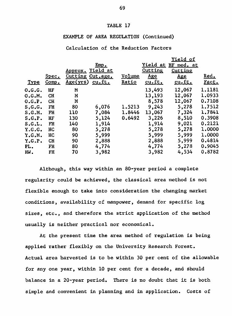
69
TABLE 17
EXAMPLE OF AREA REGULATION (Continued)
Calculation of the Reduction Factors
Yield of Emp. Yield at HF med. at
Approx. Yield at Cutting Cutting Spec. Cutting Cut.age. Volume Age Age Red.
Type Comp. Age(yrs) cu.ft. Ratio cu.ft. cu.ft. Fact. O.G.G. HF M 13,493 12,067 1.1181 O.G.M. CH M 13,193 12,067 1.0933 O.G.P. CH M 8,578 12,067 0.7108 S.G.G. FH 80 6,076 1.5213 9,243 5,278 1.7512 S.G.M. FH 110 7,084 1.8446 13,067 7,324 1.7841 S.G.P. HF 130 5,124 0.6492 3,226 8,510 0.3908 S .G .L. FH 140 1,914 1,914 9,021 0.2121 Y.G.G. HC 80 5,278 5,278 5,278 1.0000 Y.G.M. HC 90 5,999 5,999 5,999 1.0000 Y.G.P. CH 90 2,888 2,888 5,999 0.4814 PL. FH 80 4,774 4,774 5,278 0.9045 HW. FH 70 3,982 3,982 4,534 0.8782
Although, this way within an 80-year period a complete
regularity could be achieved, the classical area method i s not
flexible enough to take into consideration the changing market
conditions, av a i l a b i l i t y of manpower, demand for specific log
sizes, etc., and therefore the s t r i c t application of the method
usually is neither practical nor economical.
At the present time the area method of regulation is being
applied rather flexibly on the University Research Forest.
Actual area harvested is to be within 30 per cent of the allowable
for any one year, within 10 per cent for a decade, and should
balance in a 20-year period. There i s no doubt that i t is both
simple and convenient in planning and in application. Costs of

70
operational cruising can be reduced and records can be based on
scaled volumes and actual areas logged. The large volumes and
values of the old growth stands currently being logged can be
used to finance the high costs of road building associated with
a staggered setting pattern of logging. In addition, logging of
the large volumes in dead cedar trees k i l l e d by the f i r e of 1868,
and the snags, chunks and logs l e f t after the original logging
by the Abernethy and Lougheed company are actually considered as
salvage operations. These have been scheduled to be completed by
approximately 1970 and have not been entered directly into
either area or volume calculations presented here. It i s to be
hoped that volumes and values secured from these activities w i l l
be compensated by thinnings by 1970. Areas thinned can also be
excluded from area calculations provided there is reasonable
assurance that values of the f i n a l crop w i l l not be diminished
by thinning.
Volume Control Formulae
Austrian formula
The only assumption that had to be made for this formula
was concerned with the future or desired growing stock at the
end of the rotation. It was assumed that future plantations,
w i l l also use Douglas f i r seedlings. These plantations l i k e l y
w i l l be f i l l e d In with natural regeneration of hemlock and
cedar, to form a FH-type stand. Using the average Douglas
f i r site index value (124) for the Research Forest, the

71
empirical growing stock for a FH medium type was calculated and
inserted into the equation as the desired growing stock.
A„ _ Ga - Gr _ n n , 38.065.336 - 16.323.557 AC » I + £ - 543,790 + — 1 1 £7j— 1 1 -
815,562 gross cu. ft./year.
The increment in this case is the mean annual increment
of the total stand, obtained as total actual volume divided by
the average weighted age. Comparing this result to the average
volume value indicated by the area regulation i t appears that
the two values are very similar.
Hanzlik's formula
Data taken from Table 14 applicable to this formula are
as follows:
I - 556,615 cu. f t . 80 V _ - 18,935,319 cu. f t . mat
I i s the mean annual increment taken from the empirical yield
table at R = 80 years for each type and multiplied by the area
of the type. The values read for S.G.G., S.G.M., and S.G.P. were
corrected with the present volume ratio. Because these stands
are very close to the rotation age, i t can be assumed that they
w i l l retain the existing ratio to the empirical values for this
short period.
V"mat i s the volume of stands over 80 years of age.
The rotation used in this formula is 80 years. The
allowable cut i s :

72
18.935.319 80 774,588 gross cu. ft./year.
Although this formula i s widely used on the West Coast of
North America in the Douglas f i r type, i t has the weakness that
the mean annual increment of the presently young stands cannot
be accurately predicted for a long period of time. Also,
through improvement in silviculture and management, the mean
annual increment may be far greater than that indicated in
empirical yield tables. Therefore, for rough estimation i t
gives a satisfactory allowable cut estimate in virgin stands,
but in managed stands the answer i s usually conservative.
Kemp1s formula
The result of this formula can be greatly influenced by
the decision of the forest manager concerning the areas which
he inserts into the formula. The decision usually cannot be
made simply by considering the present age class distribution
because the actual stands may be of different sites, and pro
duce greater or lesser volumes than were presupposed by the
creation of the formula. An approximate estimation based on size
classes can substitute for the definition based on the age classes
(Kemp I, II) or a standard age and site class must be chosen and
the ages reduced accordingly. That i s , the volume of each actual
age and site class w i l l be compared to the basic age and site
class for which the corresponding age w i l l be read from the
empirical yield table.
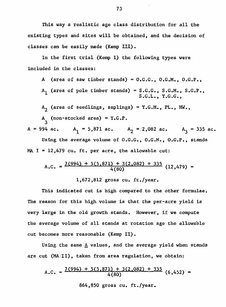
73
This way a r e a l i s t i c age class distribution for a l l the
existing types and sites w i l l be obtained, and the decision of
classes can be easily made (Kemp IX!).
In the f i r s t t r i a l (Kemp I) the following types were
included in the classes:
A (area of saw timber stands) = O.G.G., O.G.M., O.G.P.,
A^ (area of pole timber stands) = S.G.G., S.G.M., S.G.P., S.G.L., Y.G.G.,
A£ (area of seedlings, saplings) = Y.G.M., PL., HW.,
A (non-stocked area) = Y.G.P. 3
A = 994 ac. A1 - 5,871 ac. A 2 =2,082 ac. A 3 = 335 ac,
Using the average volume of O.G.G., O.G.M., O.G.P., stands
MA. I = 12,479 cu. f t . per acre, the allowable cut:
7(994) + 5(5,871) + 3(2,082) + 335 _ A.L>. - 4(80) (i-,*f/y; -
1,672,812 gross cu. ft./year.
This indicated cut i s high compared to the other formulae.
The reason for this high volume is that the per-acre yield is
very large in the old growth stands. However, i f we compute
the average volume of a l l stands at rotation age the allowable
cut becomes more reasonable (Kemp I I ) .
Using the same A values, and the average yield when stands
are cut (MA..11), taken from area regulation, we obtain:
7(994) + 5(5.871) + 3(2.082) + 335 _ A.C. - 4(80) (6,452) -
864,850 gross cu. ft./year.

74
The most logical approach for these stands may be the
third one, suggested previously.
The basic type to which a l l ages were reduced was arbi
t r a r i l y decided (HF medium). This way the selection into four
age classes with the reduced ages was more r e a l i s t i c than the
previous size selections. The new grouping,done by 20-year age
classes, i s shown below:
A ( 60+ years) O.G.G., O.G.M., O.G.P., S.G.G., S.G.M. =
2,518 reduced acres,
A^ (40-60 years) S.G.P. = 968 reduced acres,
A^ (20-40 years) = 0 reduced acres,
A ( 0-20 years) S.G.L., Y.G.G., Y.G.M., Y.G.P., PL., HW. =
4,630 reduced acres.
Here MA I was taken as the average cutting volume of old
growth stands. Introducing these values into the formula: A.C. = 7(2,518) + 5(968)^ 3(0) + 4,630 ( 1 2 > „ 9 ) .
1,056,659 gross cu. ft./year.
This cut is higher than those obtained by Hanzlik's or
the Austrian formula, but may be j u s t i f i e d for the f i r s t 10 or
20 years to eliminate the large quantities of mature volumes.
Barnes1 method
When the average age of the hardwood stands was taken as
-5 years, the average weighted age of the present stand calcu
lated from a l l the individual types gave the figure of 70 years.
Using a rotation of 80 years, the average age should have been

75
40 years, i f the stand were normal. The discrepancy is there
fore 70 - 40 = 30 years, with which the average cutting age of
the present stand w i l l have to be increased, i.e., the average
cutting age w i l l become 80 + 30 = 110 years. An estimation of
the yield at this age w i l l give the allowable cut for the present
stands.
Yields at age 110 years were read from the empirical yield
tables for each age and site class, and weighted by the area
of the class.
The f i n a l value calculated was the average weighted
yield of a l l classes at 110 years, which had to be multiplied
by the yearly reduced cutting area (A ), taken from the area
regulation method, to obtain a correct answer.
To c l a r i f y : - If l/80th of the total actual area was taken,
the average yearly cutting area would indicate a mixed, indefi
nite type, and site class. The reduced areas show an area-
equivalent of the present types and sites, as i f they a l l were
HF type, and medium site quality. In other words, the areas
were reduced to standard productivity.
The allowable cut i s :
A.C. = (Aj^ (Y 1 1 ( )) - (131.325) (6890) = 904,775 gross cu.ft./year.
An improvement of the method would be to use reduced ages
for the determination of the average present age, instead of the
actual ages. The reduced ages are obtained in a similar way

76
to that described for the Kemp III formula. These must be
weighted by the appropriate areas to obtain the correct average
reduced age for the whole area. By evaluating the new average
age we obtain 83 years, which is 13 years more than the average
age of the actual types. Hence the new estimate of the average
cutting age w i l l increase also, giving the value of 132 years.
At this age the yield of a HF medium site stand ( Y ^ ) i s 8 » 6 1 2
cu. f t . above the 11.1 inch minimum diameter, and the new
allowable cut becomes:
A.C. = (131.325) (8,612) « 1,130,971 gross cu. ft./year.
This allowable cut corresponds f a i r l y well with the one
obtained with the Kemp III formula.
Black H i l l s formula
For this formula, the following assumptions and definitions
had to be made:
1. Since in the University Research Forest there is no
marking practice at present, i t had to be assumed that a l l
volumes w i l l be taken from the presently overmature stands.
2. V was interpreted as the volume in overmature stands M
(O.G.G., O.G.M., O.G.P.) and i t was assumed that half of their
volume would be cut within the coming ten years (C^ = 0.50).
3. V became the volume of a l l other stands above minimum t
diameter limits.
4. It was assumed that l/8th of the volume of V t and half
of i t s increment during the cutting cycle would also be cut.

77
5. The period of the cutting cycle y. was taken as 10 years.
Inserting the assumed and actual values into the formula,
the allowable cut became:
10.365.840 A r = 12.404.682(0.50) 4- (25.660,654 + 2 ) 0.125
1,005,804 gross cu. ft./year,
which, in comparison with the other allowable cut estimates indi
cates a reasonable level of cut for the coming decade.
Hundeshagen's formula
On the basis of the average site and the assumed future
species composition, the desired growing stock was calculated
from the empirical yield table (Fligg, 1960), for FH medium site.
G r = 16,323,557 cu. f t . ,
whereas the actual growing stock i s
G = 38,065,336 cu. f t . a The ratio of these figures:
fa = 38,065.336 = 2.33192. G 16,323,557 r
The empirical yield at 80 years of a FH medium type stand i s :
Y = 4,774 cu. ft./acre, r The empirical yield for one year, therefore, i s 4,774 = 59.675 cu.ft,
80 Hence the actual yield per acre:
Y = (2.33192) (59.675) = 139.1573 cu. ft./year, a The total yield for the Forest, therefore, i s :
Y (total) = 9,282(139.1573) = 1,291,658 gross cu. ft./year. a The r e l i a b i l i t y of this figure - because of the inherent
78
faults of i t s assumptions - is not very high. Though, i t might
be used as an auxiliary or control for the other allowable cut
estimates.
H. A. Meyer's method
When calculating the allowable cut with this method, the
process outlined below was followed:
1. The weighted average number of trees per acre including
a l l species was calculated for each diameter class. That i s ,
the number of trees per acre of each age and site class weighted
by the actual areas they occupy.
2. The average weighted volume per acre including a l l
species was computed.
3. The average diameter growth per year including a l l
species (average of the data in Table 3) was calculated.
4. A regression equation was f i t t e d to the logarithmically-
transformed data of the average number of trees per acre calcu
lated for the whole Forest:
log N - 1.7985 - 0.05972 D.B.H.,
where N = number of trees per acre in diameter class,
D.B.H.*5 diameter at breast height in inches.
The regression equation was highly significant at the 1 per cent
level.
5. Through the substitution of the appropriate values into
the equation, given by Sammi (1960), the de Liocourt's quotient

79
was obtained (q • 1.3293).
This value was under the shown for we 11-managed Swiss
forests, and needed no reduction.
6. Knowing £ a n < i the average growth rates by diameter
classes, the per cent volume increase could be read from
Table 32 (Meyer, Recknagel and Stevenson, 1952).
7. The volume per cent read from the table multiplied by
the volume per acre value of a diameter class shows the yearly
volume increase of the class.
8. Summing up the volume increases of each diameter class
up to the desired minimum diameter limit, the yearly gross
volume increase of the stand is obtained.
9. Average yearly mortality in number of trees per acre
was calculated by diameter classes.
10. The average volume of a tree in a diameter class was obtained as average volume per acre
number of l i v i n g trees per acre*
11. The multiplication of the average volume per tree by
the number of dead trees in a diameter class gave the mortality
losses within that class.
12. The cumulative mortality losses subtracted froml-fcae
cumulative annual volume increase figures equalled the cumulative
net volume increase of the Forest in cu. f t .
13. A maximum diameter limit of 30 inches was set, beyond
which a l l trees were to be cut within a predetermined period.
14. The elimination of trees larger in diameter than 30

80
inches was set to 80 years, and also for comparative purposes
to 20 years.
15. During the elimination period, i t was assumed that a l l
the net volume increment below 30 inches in diameter, plus l/8th
(or respectively l/20th) of the volume of trees 30 inches and
larger and half of the increment of this latter class, would be
cut.
Since the necessary information for this method was calcu
lated in merchantable cubic feet, the allowable cut obtained for
the two different assumptions is also given in the same units:
A.C. = 531,585 net cu. ft./year, oO A . C 2 0 = 745,858 net cu. ft./year,
where A.C. = the yearly allowable cut, when the 80-year conversion period is used, and
A.C. = the yearly allowable cut, when the 20-year conversion period i s used.
Assuming that the cut w i l l be taken in mature stands, the
gross volumes w i l l read:
A.C. = 914,326 gross cu. ft./year, 80 A.C. 2 o = 1,282,876 gross cu. ft./year.
The possible reason for the lower estimate in the 80-year
conversion period is that the £ value might have been under
estimated as a result of the present understocked condition of
the young growth stands, or because of the use of unweighted
average growth rates.
As a f i n a l conclusion concerning the use of the method,

81
i t might be stated that, considering the long and tiresome
calculations, which are open to the risk of human error,
the effort spent in obtaining an estimation of the allowable
cut with this method is not j u s t i f i e d . Nevertheless, there
is some value in the stand table and the growth and mortality
data for their own sake as a guide to management.
Von Mantel's formula
In contrast with H. A. Meyer's somewhat complicated
method, Von Mantel's formula, often called one of "glorious
simplicity", with the substitution of only two figures, gives
the following result: . „ 2(38.065.336) 0_. _ , A.C. - — 1 rQQ
r *• = 951,633 gross cu. ft./year,
where the figure 38,065,336 means the actual growing stock in
cubic feet, and 80 i s the rotation in years.
Considering the volume distribution of the Forest (Figure
2) the allowable cut indicated by this formula should be f a i r l y
reasonable. However, because of the fast growth rate of the
young stands, and the large areas of overmature timber in need
of removal, the result might be judged somewhat conservative
for the coming decade.
Grosenbaugh's simple interest formula
The following actual and estimated values were used in
this formula:
m =10 years,
n =80 years,

82
V Q = 38,065,336 cu. f t . ,
V = 16,323,557 cu. f t . n V^, the future growing stock figure, was assumed for 80
years hence, and was read from the empirical yield table for
FH stands at medium site. G„ - 0.0093, o ' G L = 0.0289;
G was calculated from the increment values of stands o presently older than 80 years, whereas shows the growth rate
of the entire growing stock predicted for the next 10 years.
G 2 = 0.05.
This figure is an estimated value of the growth rate
expected over the 80-year period, and i s estimated to come
from the results of improved management, silviculture (thinning,
salvage, removal of slow-growing old growth stands), planting,
etc.
By substituting these figures into Grosenbaugh's formula,
the estimated allowable cut for the next decade i s :
A.C. - 38,065,336 1+80(0.05)-^;^;^ 10(0.0289) 10
1+ 2(0.00934) 1+10(0.00934) 80(0.05)
12,037,782 cu. ft./lO years, or 1,203,778 cu. ft./year.
After the f i r s t ten-year period this high indicated cut
would l i k e l y be reduced because most of the slow-growing stands
of the Research Forest w i l l be removed.

83
W. H. Meyer's amortization formula
Information needed for this formula, as applied to the
Research Forest, is li s t e d and explained below:
V D = 38,065,336 cu. f t . ,
V » 35,347,614 cu. f t . m
Assuming that 80 years hence the Research Forest w i l l have
the growing stock of a FH medium site (16,323,557 cu. f t . ) , and
in the next decade l/8th of the volume difference of the present
and desired growing stock w i l l be cut, then the future volume 10
years hence can be calculated as: The present growing stock
minus l/8th of the volume difference. I.e. ir - is n « 38.065.336 - 16.323.557 _ A 1 / . V Q = 38,065,336 - g = 35,347,614 cu. f t . ,
where n =10 years,
(l+g^* = 1.28908,
( l + g ^ = 1.0934,
-8^ - 0.009,
A.C. = 0.009 38 1065 1336(1.8908) / i35,347 1614 = ^ cu. ft./year.
Sven Petrini's interest formulae
Compound interest (I)
This formula is identical to the one which was originally
devised by W. H. Meyer in 1943, and gives a slightly lower
estimate of the allowable cut than the amortization formula
above.
Using the corresponding values of the Research Forest,

84
the following values can be substituted into the formula:
(1.0p) t = 1.28908,
k - 38,065,336 cu. f t . ,
K = 35,347,614 cu. f t . and
O.Op » 0.0257. t t Here (l.Op) , k, and K are similar to W. H. Meyer's (l+g t) ,
V and V values respectively. The only exception i s , in this o m formula, the compound interest rate of the whole stand (O.Op) is
used in the places of Meyer's g^ value, giving an allowable
cut of: A.C. - 0.0257 38,065,336a.28908)-35,347,614 _ ^ & J
year.
Since the largest ingrowth occurs in the young stands,
which at present are understocked and need to be increased
in stocking, the allowable figure given by this formula may
better f i t the actual situation than the improved W. H. Meyer's
amortization formula.
Simple interest formula (II)
Using the values of the Research Forest the following
figures were substituted into the formula:
t «= 10 years,
p = 2.8908 per cent,
k - 38,065,336 cu. f t . ,
K » 35,347,614 cu. f t . , and
tt+mn> - L28908,

85
hence, the allowable cut i s :
_ 38.065.336 (1.28908) - 35.347.614 A.C. = 10 1 + 10 (2.8908)
200 + 10 (2.8908) 1,218,306 cu. ft./year,
This figure, from the management point of view, is identical to
the one obtained by the compound interest formula, and the
fi n a l comments made previously apply to the simple interest
formula as well.
Area and Volume Control Methods
Area-volume computation
This is a method adapted for the use of empirical yield
tables, from the Reports of the West Coast Forest Procedures
Committee (1950).
The method starts out stating the types, present ages,
and actual and reduced areas, as in the area regulation, and
must be accompanied by an approximate yearly cut figure obtained
from one of the allowable cut formulae.
Then a preliminary estimate is obtained of the cutting
age and total yield for each age and site class, in a similar
way to that described in the area method. This estimate of the
total yield is divided by the preliminary allowable cut figure,
to see how long this volume w i l l last, i f this preliminary
figure were cut each year. When half of the duration period i s
added to the age when cutting starts, the sum w i l l give the
f i n a l cutting age of the age and site class in question. At
this age the yield is read from the empirical yield table

86
(for S.G.G., S.G.M., S.G.P., yields are corrected by the present
volume ratio) and multiplied by the actual acres of the type.
Finally this volume, divided by the preliminary allowable cut,
w i l l give the f i n a l duration of the cut within that class,
which then is added to the cumulative column of the table.
Turning to the next age and site class, the i n i t i a l
cutting age i s obtained, when the last figure of the cumulative
age column is added to the present age of this class. A l l
further calculations from here on proceed as described above.
If the f i n a l figure in the cumulative age column is
within the range of the desired limit R(l*0.05), then the pre
liminary allowable cut figure i s acceptable. If not, a new
allowable cut estimate must be set, making the new estimate
higher, when the f i n a l cumulative age was high, or lower, i f
It was low, and the process repeated accordingly.
For the Research Forest the f i r s t estimate of 870,000 cu.
f t , of the allowable cut proved to be low. With a second t r i a l
figure of 970,000 cu. f t . , the f i n a l figure of the cumulative
column was within the limit, but lower than the rotation age
(77 years). Taking this into consideration, the 970,000 cu. f t .
was lowered to 960,000 cu. f t . and accepted as the fi n a l estimate.
The method i s presented in detail in Table 18.

87
TABLE 18
EXAMPLE OF AREA-VOLUME COMPUTATION,
USING PRELIMINARY ALLOWABLE CUT ESTIMATE OF 970,000 cu. f t 0
Yield Cut Yield Actual Per Actual
Avg. Begins Ave. per acre Approx. Avg. Acre Yield Actual Actual at Cut. When Yield Cut. When When Years
Spec. Site Age Area Red. Age Age Cut When Cut Age Cut Cut to Cut Type Comp. Class yrs. ac. R. F» Acres yrs. yrs. cu.ft. M.cu.ft. yrs. cu.ft. cu.ft. Per. Cum. O.G.G. HF G M 159 1.118 178 M M 13,493 2,140 M 13,493 2,145,387 2.2 2.2 O.G.M. CH M M 671 1.093 734 M M 13,193 8,850 M 13,193 8,852,503 7.1 11.3 O.G.P. CH P M 164 0.711 117 M M 8,578 1,380 M 8,578 1,388,096 1.4 12.7 S0GoGo FH G 70 805 1.751 1,410 83 88 10,504 8,470 87 10,346 8,328,530 8.6 21.3 S.G.M. FH M 80 1,885 1.784 3,363 101 114 13,550 25,500 114 13,609 25,652,965 26.5 47.8 S. G. P o HF P 90 968 0.391 378 138 139 3,510 3,350 140 3,512 3,339,616 3.4 51.2 S. G oL o FH L 90 43 0.212 9 141 141 1,925 80 141 1,925 82,775 0.1 51.3 Y.GoG a HC M 30 2,170 1.000 2,170 81 90 5,963 12,900 88 5,847 12,687,990 13.1 64.4 YoG.Mo HC M 25 1,171 1.000 1,171 89 94 6,278 7,340 93 6,222 7,285,962 7.5 71.9 Y o G o P o CH P 20 335 0.481 161 82 83 2,541 850 82 2,519 843,865 0.9 72.8 PL. FH M 5 558 0.904 505 78 80 4,750 2,650 79 4,702 2,623,716 2.7 75.5 HW. FH M -5 353 0.878 310 71 72 4,117 1,450 71 4,077 1,439,181 1.5 77.0
10,506
YEARLY CUTTING AREA: 10,506 : 80 = 131.325 reduced acres

88
Area-volume allotment
As a necessary step to begin the calculations, the cutting
cycle had to be chosen, for which the allowable cut w i l l be
calculated. This was set at ten years, which is comparable to
the period for some of the other calculations.
In this method, the same types, actual ages, actual and
reduced areas were used as in the area regulation, or as in the
area-volume computation. The reduced cutting area during the
cutting cycle became ten times the size of the one year cutting
area, giving a figure of 1,313 reduced acres. The reduced areas
of the condition classes, l i s t e d in their order of cutting
sequence, were added u n t i l the sum was equal to 1,313 acres.
The next step was to set the average cutting age of the age
and site classes, at which the yields had to be found in the
empirical yield table. This age was assumed to be equal to the
i n i t i a l age plus half of the cutting cycle (5 years) for the
f i r s t period, and the i n i t i a l age and one and one-half cutting
cycles (15 years), for the second period. At this age, the
yields read from the empirical yield table represented the
f i n a l yields of the age and site class. (At this point i t must
be noted that similarly to the area regulation and to the area-
volume computation, for the old growth stands, the present
volumes were assumed as cutting volumes. For the second growth
stands the future empirical yields were multiplied by the

89
present volume ratios, assuming that this ratio w i l l remain
constant during the next five- or fifteen-year period.) The sum
of the volume per acre figures multiplied by the actual areas
of the age and site classes gave the total gross cubic foot
volumes cut during the cutting cycles. As a result of the large
harvest volumes in the old growth stands, in the f i r s t cutting
cycle nearly twice as much volume appeared as in the second,
which was composed of second growth stands. To moderate the
large volume differences occurring between the two cutting
cycles, the total yields obtained for the two cycles were
averaged and the corresponding reduced acres recalculated.
Obviously, the reduced acre values became lower in the f i r s t
cycle and larger in the second, as a consequence of the equa
lized volume cut figure.
It is essentialfbr the method that before the f i r s t
cutting cycle ends, a new allocation is carried out, using the
age and site classes presently in the second cutting cycle, and
the ones f a l l i n g into the third decade of the regulation. This
way a gradual equalization of the volumes and cutting areas is
brought about; thus a continuous trend towards normality can be
achieved, with less sacrifice than i t would be using a pure area
regulation. (See detailed calculations in Table 19.)
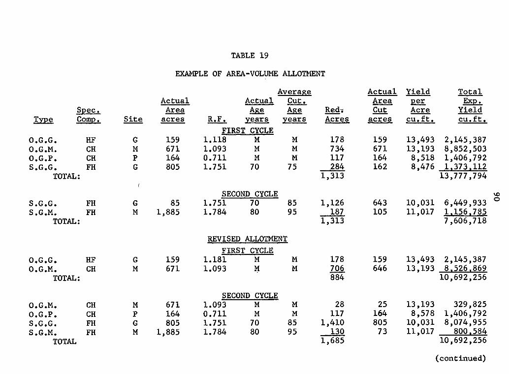
TABLE 19
EXAMPLE OF AREA-VOLUME ALLOTMENT
Average Actual Yield Total Actual Actual Cut. Area per Exp.
Spec. Area Age Age Red? Cut Acre Yield Type Comp. Site acres R.F. years years Acres acres cu.ft. cu.ft.
FIRST CYCLE O.G.G. HF G 159 1.118 M M 178 159 13,493 2,145,387 O.G.M. CH M 671 1.093 M M 734 671 13,193 8,852,503 O.G.P. CH P 164 0.711 M M 117 164 8,518 1,406,792 S.G.G• FH G 805 1.751 70 75 284 162 8,476 1.373.112
TOTAL: 1,313 13,777,794 f SECOND CYCLE
S.G.G• FH G 85 1.751 70 85 1,126 643 10,031 6,449,933 S.G.M. FH M 1,885 1.784 80 95 187 105 11,017 1.156.785
TOTAL: 1,313 7,606,718
REVISED ALLOTMENT FIRST CYCLE
O.G.G. HF G 159 1.181 M M 178 159 13,493 2,145,387 O.G.M. CH M 671 1.093 M M 706 646 13,193 8,526,869
TOTAL: 884 10,692,256
SECOND CYCLE O.G.M. CH M 671 1.093 M M 28 25 13,193 329,825 O.G.P. CH P 164 0.711 M M 117 164 8,578 1,406,792 S.G.G. FH G 805 1.751 70 85 1,410 805 10,031 8,074,955 S.G.M. FH M 1,885 1.784 80 95 130 73 11,017 800.584
TOTAL 1,685 10,692,256
(continued)

91
TABLE 19 (Continued)
EXAMPLE OF AREA-VOLUME ALLOTMENT
10-year CUTTING AREA » 1 ° ^ 5 0 6 = 1,313.25 acres
AVERAGE YIELD = A.C. - 13,777,794+7,606,718 =
10,692,256 gross cu. ft./lO years

92
CONCLUSION
Before considering the results obtained from this study,
i t must be emphasized that for practical allowable cut e s t i
mates a statistically-planned sampling to a required level of
confidence would be essential.
When planning a more intensive inventory, data obtained
with this small scale survey could be used profitably for the
calculation of the necessary number of measurements in each phase s
(number of point samples, number of increment cores, height
measurements, etc.).
Further divisions of the present classes into more detailed
age classes and stocking classes would also be advisable.
This thesis did not involve the calculation of actual
sampling errors, as would be necessary for practical purposes.
It simply stressed the importance of calculating and applying
several allowable cut methods to a forest, and developing an
inventory procedure, where the necessity of such allowable cut
estimations arises.
This importance can be realized i f we take a look at the
f i n a l summary table of the allowable cut calculations (Table 20),
where the calculated allowable cut volumes are presented in
gross and net merchantable cubic feet. It was assumed that cuts
would be taken from the old growth stands in the coming ten years

93
and when calculating net merchantable volumes, corresponding
merchantable reduction factors were therefore used. Factors
are given in Table 14. It should be noted that no allowances
have been made for research reservations or possible additions
to the area of the Forest.
Except S. Petrini's two formulae - which are based on the
same principles - a l l methods show different answers, caused by
the difference in their basic assumptions, or by their applica
tion to a certain condition. Naturally in this case a simple
s t a t i s t i c a l comparison of these figures would not be r e a l i s t i c .
They have to be judged by considering many aspects of the pre
vailing forest management methods, present condition of stands,
and possible future improvements. Most of these aspects were
touched upon in the general description of the formulae and
further elaborated and commented on in the discussions of the
actual calculation.
Some points, however, need further explanation. It i s seen
from Figure 2 that volume distribution in the Research Forest is
far from normal. The cruise data used in this study showed that
old and second growth stands are overstocked, whereas the younger
20-30-year age classes are understocked by comparison with
Fligg's (1960) estimates. (See reduced age distribution in the
calculation of the Kemp III formula.) Obviously the objects of
management w i l l be to reduce these irregularities in the shortest
time with the least sacrifice. Pure area regulation would be the

94
easiest way to attain normality, but this would result in large
harvest volume differences during the f i r s t rotation. Errors
in the estimation of future yields could also appear from the
determination of sites and areas of presently young, understocked
stands. These stands, during the long estimation period,
might not develop to the level of the empirical yields, as
expected. These uncertainties naturally can be corrected and
empirical yields exceeded by employing intensive s i l v i c u l t u r a l
practices, together with regular checks on the stands, recurrent
inventories, and by using short yield prediction periods.
In contrast to area regulation, volume methods w i l l
result in even yearly or periodic harvest volumes, but this
way the trend towards a normal forest w i l l slow down. For
example, allowable cut volumes (Table 18), calculated from
volume formulae, gave much lower estimates than are indicated
for the f i r s t eight years in the area regulation method (see
area regulation calculations).
It must also be noticed that formulae based on periodic
annual increments show higher allowable cut volumes than
formulae based on mean annual increment. These might be con
sidered as slight overestimates, since i f the young growth
stands are presently understocked, i t follows that their incre
ment should not be allocated for cutting, rather, i t should be
considered on the account of stocking improvement.

95
DoB.H, GROSS NET Limit
i n . Area Regulation 3.1 9.1 910,494 529,197 11.1 847,284 491,967 13.1 813,557 471,832
Barnes I 3.1 1,042,174 602,918 9.1 971,481 654,644 11.1 904,775 525,348 13.1 827,501 479,512
Grosenbaugh 3.1 9.1 1,502,849 873,486 11.1 1,203,778 698,962 13.1 1,035,659 600,133
Area-Volume Allotment 3.1 9.1 1,088,324 632,556 11.1 1,069,226 620,835 13.1 976,641 565,934
TABLE 20
YEARLY ALLOWABLE CUT VOLUMES AS CALCULATED BY DIFFERENT FORMULAE AND METHODS
YIELD IN CUBIC FEET
GROSS NET
Austrian
880,137 511,553 815,562 473,548 733,746 448,362
Barnes II 1,246,799 721,298 1,199,917 697,415 1,130,971 656,687 1,048,761 627,725
Wo H. Meyer
1,603,836 932,181 1,321,528 767,332 1,142,362 661,964
GROSS NET
Hanzlik 958,334 554,415 846,289 491,880 774,588 449,757 692,997 401,571
Hundeshagen 1,468,112 849,332 1,319,442 766,886 1,291,658 749,988 1,211,506 702,031
Petrini I
1,462,456 850,009 1,219,892 708,318 1,063,511 616,273
GROSS NET
Kemp I
1,692,972 983,989 1,672,812 971,301 1,635,334 947,627
H0 A. Meyer I 1,085,543 631,130 1,018,176 591,963 914,326 531,585 783,265 455,387
Petrini II
1,462,249 849,888 1,218,306 707,397 1,060,924 614,774
GROSS NET
Kemp II
932,810 542,168 864,850 502,166 780,537 452,298
H. A. Meyer II f,449,103 842,502 1,386,559 806,139 1,282,876 745,858 1,151,917 669,719
Black H i l l s
1,077,848 626,467 1,005,804 584,010 932,861 540,565
GROSS NET
Kemp III
1,069,445 621,583 1,056,659 613,538 1,033,035 598,613
Von Mantel 1,263,218 730,797 1,048,681 609,514 951,633 552,556 847,278 490,972
1,035,783 602,018 960,000 557,414 884,205 512,370
Area-Volume Computation

96
As a transition between the area regulation and the volume
formulae, the area-volume control methods gave a more or less
in-between answer concerning cutting volumes, simultaneously
ensuring a continuous trend towards a normal forest.
In consideration of which method actually is to be used,
the general objectives of management of any property must be
known. For the University Research Forest, these were stated by
the U.B.C. Forest Committee in 1959 as: "The University Forest
is managed to provide a sustained and maximum income. This
management is to be consistent with effective use of the property
for teaching, demonstration, research, and public recreation.
Income from the Forest w i l l be used to maintain the capital
value of the Forest in such a manner that these prime uses w i l l
be maximized."
Since a l l forest products from the University Research
Forest are sold on the open market there i s no need to consider
the special problems that might arise i f demands of a particular
manufacturing plant had to be satisfied.
From the regulation point of view a decision should be made
as to what level of cut can be sustained and at the same time
provide a maximum income indefinitely into the future.
The high allowable cut values suggested by the Grosenbaugh,
W. H. Meyer, H. A. Meyer II, and Petrini formulae are the result
of application of approaches that are not suited to the present
intensity of management of the Forest. Their application would

97
assume salvage of dead trees and thinning regimes not yet practic
able. The present large surplus of big trees makes d i f f i c u l t
the application of systems based on diameter distributions.
The period over which surplus volumes are to be harvested would
depend very much on the objectives of management. It ranges
from several decades to a whole rotation in different methods.
From the economic point of view existing old growth volumes
should be harvested as rapidly as possible to provide the capital
for development of roads and improvement of amount and value of
growth on the whole forest. This suggests the use of a short
period of adjustment but requires careful planning of the transi
tion from logging of old growth to logging of younger stands.
In this regard the surplus of stands above rotation age w i l l
f a c i l i t a t e the transition and the road system developed for
logging of old growth w i l l provide an excellent basis for more
intensive management of young stands.
It i s obvious that without intensive management, average
volumes harvested per acre must decrease. If intensive manage
ment can be j u s t i f i e d economically and applied immediately, the
level of cut eventually might approach that indicated by simple
area regulation for the next two decades.
The most conservative formula (Hanzlik) allocates surplus
growing stock over the rotation, and uses mean annual increment
at 80 years. These assumptions should be subject to review as
conditions change.

98
It is obvious that none of the foregoing formulae or methods
can be selected as absolutely correct. However, area-volume
control methods seem to provide the most r e a l i s t i c approach as
a compromise between pure area and volume approaches.
If the area-volume computation and the area-volume allotment
methods are compared, the allowable cut obtained by the area-
volume allotment w i l l show a figure approximately 100,000 gross
cu. f t . higher for the next decade. This presents the problem
of choosing the level of cut which is better suited to the condi
tion of the Forest. Before the f i n a l decision is made, the
possible development of the 30-year-old stands on the Forest
also should be discussed.
Parts of the Research Forest now covered by the presently
30-year-old stands were burned in the years 1925, 1926 and 1931
(Walters and Tessier, 1960). After the burning and u n t i l 1953,
this area was l e f t to Nature without any provision for a r t i f i c i a l
restocking. In 1953, forestry students planted a few acres of
the understocked areas with Douglas f i r , Scots pine and Norway
spruce. Restocking to reasonably satisfactory levels, however,
was completed in 1959, when the last large poorly stocked
area was planted with 6,500 Douglas f i r seedlings and 6,000
Scots pine seedlings on 117 acres. In a l l , more than 90,000
seedlings were planted on 700 acres. Stocking probably w i l l
continue to improve as a result of natural regeneration.

99
Because the A.&L. portion of the Forest i s in the i n i t i a l
stages of planned management, there are s t i l l large areas which
have volumes well below Fligg 1s (1960) empirical volume e s t i
mates, and their complete recovery cannot be expected within
the coming 10 or 20 years. Although Fligg 1s data may be
misleading because of curving at lower ages, the problem of
indicated understocking remains. In spite of the efforts spent
on regeneration, caution must therefore be used when calculating
the allowable cut for the coming two decades. A supplementary
volume regulation formula, which bases i t s estimate on actual
volumes, may be used as a guide for the selection of a f a i r l y
safe allowable cut estimate from the two favoured area-volume
method. For this purpose Von Mantel's formula should provide
a reasonable comparison. Fortunately the allowable cut obtained
by Von Mantel's formula is almost identical to that obtained
by the area-volume computation method and thus verifies the
f i n a l selection of the allowable cut indicated by the area-
volume method.
Naturally, as time passes, more experience w i l l be gained,
more w i l l be learned about the Forest and more intensive s i l v i
cultural and u t i l i z a t i o n techniques w i l l be applied. Although
rotation length has been assumed to average 80 years, this may
not be optimum. It i s hoped i t can be reduced by improving
standards of u t i l i z a t i o n and more intensive management. It is
thus reasonable to expect that the growth and yield of the

100
Research Forest w i l l increase. However, at the present stage
a short prediction period and a method providing a moderately
conservative allowable cut should be used.
When complete recovery of the presently understocked
areas is assured, the use of the simpler area-volume allotment
method may be more convenient. However, u n t i l then i t would
appear safer to use the area-volume computation method, which
gives a lower allowable cut.

101
BIBLIOGRAPHY
Allen, R. H. Jr. and E. W. Morgen. Range mean ratio of basal area as an indicator of B i t t e r l i c h sampling intensity in lodgepole pine." College of Forest and Range Management, Colorado State University. Fort Collins, Colorado. Research Note No. 13. 2pp.
Allison, G. W. and R. E. Breadon. 1960. Timber volume e s t i mates from aerial photographs. For. Survey Notes. No. 5. Department of Lands and Forests. Victoria, B. C. 25pp.
Bajzak, D. 1960. Forest inventory on aerial photographs of part of the University of Bri t i s h Columbia Research Forest, Haney, B. C. University of Bri t i s h Columbia, Faculty of Forestry. Vancouver 8, B. C. Unpublished report. 11pp.
. 1960. An evaluation of site quality from aerial photographs of the University of Bri t i s h Columbia Research Forest, Haney, B. C. University of Bri t i s h Columbia, Faculty of Forestry, M.F. thesis. Vancouver 8, B. C. 113pp.
Baker, F. S. 1960. A simple formula for gross current annual increment. Jour. For. 58(6):488-489.
Barnes, G. H. 1951. A new method of volume regulation. Jour. For. 49(4):272-277.
B e l l , J . F. and L. B. Alexander. 1957. Application of the variable plot method of sampling forest stands. Oregon State Bd. of Forestry. Forest Research. Note 30. 21pp.
Briscoe, C. B. 1957. Stand table construction from relascope plots. La. Agr. Exp. St. Forestry. Note 15. 3pp.
Castles, J. R. 1959. Calculating allowable harvest cuts in the National Forests of the Northern Rocky Mountain Region. Society of American Foresters. Proceedings. Society of American Foresters meeting. Mills Building, Washington 6, D.C. pp.109-151.
Chapman, H. H. 1950. Forest Management. The Hildreth Press Publishers. B r i s t o l , Conn. 582pp.

102
Cunia, T. 1959. Notes on cruising intensity by the B i t t e r l i c h method. Jour. For. 57(11):849-850.
Davis, K. P. 1954. American Forest Management. McGraw-Hill Book Co. Inc. Toronto. 482pp.
Fekete, Z. 1950. Erdorendezestan. Agrartudomanyi Egyetem Erdo- es Foldmernoki Kar. Sopron. Hungary. 133pp. Mimeo.
Fligg, D. M. 1960. Empirical yield tables. Forest survey notes. No. 6. Br i t i s h Columbia Forest Service, Department of Lands and Forests. Victoria, B. C.
Greeley, A. W. 1935. Development of management plans on Snoqualmie National Forest. Yale University. School of Forestry, M.F. thesis. 155pp.
Grosenbaugh, L. R. 1952. Plotless timber estimates...new, fast, easy. Jour. For. 50(1):32-37.
j_ 1955. Better diagnosis and prescription in Southern Forest Management. Southern For. Expt. Sta. Occasional paper. 145. 27pp.
j_ 1958. Allowable cut as a new function of growth and diagnostic t a l l i e s . Jour. For. 56.(10): 727-730.
1958. Point-sampling and line-sampling: Probability theory, geometric implications, synthesis. Southern For. Expl. Sta. Occasional paper. 160. 34pp.
Gross, L. S. 1950. Timber Management Plans on the National Forests. U. S. Dept. of Agr. Washington 25, D.C. 59pp.
Hanzlik, E. J. 1922. Determination of the annual cut on the sustained basis for virgin American forests. Jour. For. 20(6):611-626.
Hough, A. F. 1954. The control method of forest management in an age of aerial photography. Jour. For. 52(8):568-574.
Hughes, W. G. 1956. Management plan considerations in i n i t i ating sustained yield forestry. The Empire Forestry Review. 35(1):29-35.
Jerram, M. R. K. 1945. A Textbook on Forest Management. Chapman and Hall Ltd. London. 154pp.

103
Johnson, F. A. and V. E. Hicks. 1956. Estimating allowable cut without a type map in forests of Western Washington and Western Oregon. Jour. For. 54(8):522-524.
j_ 1961. Standard error of estimated average timber volume per acre under point sampling, when trees are measured for volume on a subsample of a l l points. U. S. Dept. of Agr. Pac. Northern For. and Range Expt. Sta. Res. Note. No. 201. 5pp.
Kendall, R. H. and L. Sayn-Wittgenstein. 1959. An evaluation of the relascope. Canada Dept. of Northern Affairs and Natural Resources. For. Research Div. Tech. Note. No. 77. 26pp.
Ker, J. W. 1953. Growth of immature Douglas f i r by treeaclasses. For. Chron. 29:367-373.
j_ and J. H. G. Smith. 1957. How much and how fast — forest measurements today. British Columbia Lumberman. February and March. 6pp.
t J. H. G. Smith, and J. Walters. 1957. Observations on the accuracy and u t i l i t y of plotless cruising. British Columbia Lumberman. November. 2pp.
Littleton, D., A. Strother, H. Eidsvik and T. Jeanes. 1957. Re-appraisal of the allowable annual cut on the U.B.C. Research Forest, Haney, B. C. University of British Columbia, Faculty of Forestry. Vancouver 8, B. C. Unpublished report. 6pp.
Meyer, H. A., A. B. Recknagel and D. D. Stevenson. 1951. Forest Management. The Ronald Press Co. New York. 290pp.
•_ 1952. Structure, growth and drain in balanced uneven aged forests. Jour. For. 50(2):85-92.
s_ 1952. Accuracy of forest growth determination based on the measurement of increment cores. Agr. Expt. Sta. State College, Pennsylvania. Bulletin 547. 25pp.
Meyer, W. H. 1943. Amortization in stand growth and depletion problems. Jour. For. 41(12):920-922.
j_ 1952. Regulation of cut in immature understocked forests. Jour. For. 50(12):934-939.

104
Petrini, S. 1956. Determining the possible yield. Bulletin No. 21. Royal School of Forestry. Stockholm, Sweden. 9pp.
Recknagel, A. B. 1917. The theory and practice of working plans. John Wiley and Sons. New York, N. Y. 265pp.
Robertson, R. C. and J. N. MacFarlane. 1960. Growth in volume and value on the U.B.C. Research Forest during the next decade. University of British Columbia, Faculty of Forestry. Vancouver 8, B. C. Unpublished report. 13pp.
Sammi, J. C. 1961. De Liocourt's method modified. Jour. For. 59(4):294-295.
Smith, J. H. G. 1952. A c r i t i c a l appraisal of methods of forest regulation. Yale School of Forestry, Directed Study. 146pp. typed.
t and J. W. Ker. 1957. Timber volume depends on D2H. Bri t i s h Columbia Lumberman. September. 2pp.
1958. Management planning and determination of the allowable cut in forests of the United States and Canada. The Empire Forest Review. 37.(91):43-48.
^ and J. W. Ker. 1959. Empirical yield equations for young forest growth. British Columbia Lumberman. September. 2pp.
j_ J. W. Ker and J. Csizmazia. 1961. Economics of Douglas f i r , western hemlock and western red cedar in the Vancouver Forest D i s t r i c t . The University of Bri t i s h Columbia. Vancouver 8, B. C. Forestry bulletin No. 3. 144pp.
Spurr, S. H. 1952. Forest Inventory. The Ronald Press Co. New York, N.Y. 476pp.
j . 1954. Simplified computation of volume and growth. Jour. For. 52(12):914-922.
s_ 1960. Photogrammetry and photo interpretation. Second Edition of Aerial Photographs in Forestry. The Ronald Press Co. New York, N.Y. 472pp.
Stage, A. R. 1959. A cruising computer for variable plots, tree heights and slope correction. Jour. For. 57(11): 835-836.

105
Stage, A. R. 1960. Computing growth from increment cores with point sampling. Jour. For. 58(7):531-533.
The Western Forestry and Conservation Association. 1950. Reports of the West Coast Forestry Procedures Committee on various recommended practices and techniques. Portland, Oregon.
University of Br i t i s h Columbia Research Forest Committee. 1959. The f i r s t decade of management and research on the U.B.C. Forest, 1949-1958. University of B r i t i s h Columbia. Vancouver 8, B. C. 82pp.
University of British Columbia Forest Club. 1959. Forestry Handbook for British Columbia. Second edition. University of Br i t i s h Columbia Forest Club. Vancouver 8, B. C. 800pp.
U. S. Dept. of Agriculture. 1958. Explanatory notes on the allowable cut task force report. Forest Service, Washington, D.C. 63pp.
Walters, J. and J. P. Tessier. 1960. U.B.C. researchers put "A.&L." back in production. British Columbia Lumberman. December. 3pp.
Yoder, R. A. 1961. Accumulation and processing data for decision making in forest management. Proceedings. Sixteenth Yale Industrial Forestry Seminar, Oregon State College. Corvallis, Oregon. 12pp.