a comparative study on evaluation methods of fluid forces

Research ArticleA Comparative Study on Evaluation Methods of Fluid Forces onCartesian Grids

Taku Nonomura12 and Junya Onishi3

1 Institute of Space and Astronautical Science Japan Aerospace Exploration Agency Yoshinodai 3-1-1 1816Sagamihara Kanagawa Japan2Department of Aerospace Engineering Tohoku University Sendai Miyagi Japan3Institute of Industrial Science The University of Tokyo 7-1-26 Minatojima-minimi-machi Chuo-ku Kobe Hyogo Japan

Correspondence should be addressed to Taku Nonomura nonomuraaeromechtohokuacjp

Received 7 April 2017 Revised 31 May 2017 Accepted 14 June 2017 Published 19 July 2017

Academic Editor Rahmat Ellahi

Copyright copy 2017 Taku Nonomura and Junya Onishi This is an open access article distributed under the Creative CommonsAttribution License which permits unrestricted use distribution and reproduction in any medium provided the original work isproperly cited

We investigate the accuracy and the computational efficiency of the numerical schemes for evaluating fluid forces in Cartesiangrid systems A comparison is made between two different types of schemes namely polygon-based methods and mesh-basedmethods which differ in the discretization of the surface of the object The present assessment is intended to investigate the effectsof the Reynolds number the object motion and the complexity of the object surfaceThe results show that themesh-basedmethodswork as well as the polygon-based methods even if the object surface is discretized in a staircase manner In addition the resultsalso show that the accuracy of the mesh-based methods is strongly dependent on the evaluation of shear stresses and thus theymust be evaluated by using a reliable method such as the ghost-cell or ghost-fluid method

1 Introduction

In recent years Cartesian grids have been widely used incomputational fluid dynamics applications This is not onlybecause of the simplicity of data structure and algorithms butalso because of the fast automatic and robust grid generationfor complex geometries The latter reason is particularlyimportant for industrial applications since grid generation isone of the most time-consuming tasks Cartesian grids havepotential to overcome this difficulty

However flow simulation using Cartesian grids still hassome issues to be addressed before being put into practiceA key issue is the development of accurate methods forevaluating physical quantities and fluxes at the surface of solidobjects This issue comes from the fact that Cartesan gridsdo not necessarily align with the surface of the objects As aresult there arises some arbitrariness in the location and theorientation of the object surfaces and thus the evaluation ofphysical quantities and fluxes at the object surface is highlydependent on the numerical schemes used To improve the

numerical evaluation described above many efforts havebeen already devoted since the pioneering work by Peskin[1] An extensive review of the methods developed in theliteratures is given by Mittal and Iaccarino [2]

Despite these efforts however there has been no estab-lished method that can be applied to any problems Thisis partly due to the lack of the systematic investigationon the accuracy of the numerical schemes used in thesemethods In this study we assess and compare the accuracyand the computational efficiency of the numerical schemesfor evaluating physical quantities and fluxes in Cartesian gridsystems In particular we focus on the evaluation of the localfluid stresses at the surface of an object and on the evaluationof the total fluid forces acting on the object body as theintegration of the local stresses

The fluid force acting on a solid body is evaluated byintegrating the fluid stresses over the body surface

119865119895 = intΓ119878

120590119894119895119899119894119889119878 (1)

HindawiMathematical Problems in EngineeringVolume 2017 Article ID 8314615 15 pageshttpsdoiorg10115520178314615

2 Mathematical Problems in Engineering

(a) Body-conforming grid (b) Nonconforming grid

Figure 1 Examples of body-conforming and nonconforming grids

where120590119894119895 is the stress tensor and 119899119895 is the unit outward normalof the surface element The stress tensor 120590119894119895 of Newtonianfluids is given by

120590119894119895 = minus119901120575119894119895 + 120583(120597119906119895120597119909119894 +

120597119906119894120597119909119895) (2)

where119901 is the pressure 119906119894 is the velocity and120583 is the viscosityIn numerical computations the surface integral defined

by (1) is evaluated in two steps

(i) discretization of the surface(ii) estimation of the physical quantities at the surface

The numerical procedures to conduct these steps depend onthe grid system used in the simulation In body-conformingcurvilinear grid systems shown in Figure 1(a) both steps canbe implemented on the specified grids in a straightforwardmanner However in nonconforming grid systems shownin Figure 1(b) some special treatment is required since thegrids do not exactly match the body surface To the best ofour knowledge there are two different ways which have beenadopted in nonconforming grid systems namely the controlvolume method and the direct calculation

The control volume method introduces a virtual volumewhich encompasses the body and estimates the fluid forcesfrom the net momentum flux through the surface of this vir-tual volume This method was firstly applied to steady forcesby Lai and Peskin [3] and later it was extended to unsteadyforces by Balaras [4] and to moving body problems by Shenet al [5] The control volume method has an advantage thatit is unnecessary to directly handle the complex geometriesexpressed by the immersed boundaries On the other handit has a severe disadvantage that local stresses cannot becomputed that is only the total force acting on the body canbe evaluated Moreover the contributions from pressure andviscous forces cannot be evaluated separately

In the direct calculation the body surface is usuallydiscretized by a set of polygons and the local stresses on these

surface elements are estimated Then the local stresses areintegrated over the body surfaces to obtain the total forceas in body-conforming grid systems However unlike thecases of body-conforming grid systems the estimation of theflow variables on the surface elements is not straightforwardand requires elaborate interpolation andor extrapolationmethods in order to accurately take into account the location(and orientation if necessary) of the surface Moreover thecomputational cost of the stress integration may becomeprohibitive when the body shape is complex since it dependson the number of the polygons used to express the bodysurface Such a dependency is undesirable in particular inengineering applications For example the number of thepolygons reaches up to the order of 107 for an aerodynamicsimulation using a detailed car model with both exterior andinterior parts [6]

In this study we discuss numerical schemes that aresuitable for evaluating fluid forces in nonconforming gridsystems In particular we propose a simple and computa-tionally efficient method for calculating the surface integralin (1) The proposed method is a kind of direct calculationdescribed above Therefore it has inherited an advantageover the control volume method in that the contributionsfrom pressure and viscous forces can be evaluated locally andseparately Moreover in the presentmethod the fluid stressesare integrated over the mesh faces (staircase surfaces) in thegrid system used not over the discretized surface elementsof the original body Therefore the undesirable dependencyon quality or numbers of surface polygons can be removedHereafter the present method is referred to as a ldquomesh-basedscheme (MS)rdquo whereas the method based on the integrationover surface polygons is called a ldquopolygon-based scheme(PS)rdquoWepresent a comparative study of the accuracy of thesemethods

It is worth noting here that in both mesh-based andpolygon-based schemes the physical quantities at the dis-cretized surfaces must be estimated by interpolation orextrapolation and the accuracy of this estimation would

Mathematical Problems in Engineering 3

influence the final results of the fluid forces For the PS wehave employed the ghost-cell approach described by Mittalet al [7] For the MSs we have tested three approaches thatare often used in the studies of immersed boundarymethodsa staircase approach a ghost-cell approach and a ghost-fluidapproach the details of which are described in Section 2

The rest of the paper is organized as follows Section 2describes the details of the computational procedures of apolygon-based scheme and three mesh-based schemes Thecomputational grid the discretization of the body surfaceand the extrapolation method used in these schemes are fullydiscussed In Section 3 both polygon-based and mesh-basedschemes are applied to evaluate the drag force acting on asphere in Stokes flow The obtained results are comparedwith the analytical solution The grid convergence test isalso performed to investigate the numerical accuracy of theschemes Stokes flow is used here because analytical solutionsare available not only for the fluid forces but also for theflow fields that is pressure and velocity fields By using theanalytical solutions of the flowfields the error associatedwiththe force evaluation schemes can be assessed separately fromthe error in the computation of the flow fields themselvesIn contrast in higher Reynolds number flows the flow fieldsmust be numerically computed Therefore these errors arehardly evaluated separately In Section 4 the extension tothe moving body problem and the computational efficiencyof the force evaluation schemes are discussed In additionto show the applicability of the present mesh-based schemein higher Reynolds number flows the results for the caseof the Reynolds number of 100 are presented in Section 5In Section 6 the discussion on the applicability to thecomplex body problem is conducted Finally the last sectionsummarizes this study

2 Numerical Methods

Herein Section 21 describes the computational grid anddefines the cell types The polygon-based force evaluationscheme which seems to be commonly used in the immersedboundary method and the mesh-based force evaluationscheme proposed in this paper are described in Sections 22and 23 respectively

21 Computational Grids andDefinition of Cell Type Thegridsystem used in this work is illustrated in Figure 2 In thisfigure the entire domain is divided into equally sized cubiccells These cells are classified into two groups according totheir locations

(i) fluid cells (cells whose center is in the fluid region)(ii) solid cells (cells whose center is in the solid region)

Within these categories special cells close to the interface aredefined as follows

(i) boundary cells (fluid cells adjacent to at least one solidcell)

The flow properties used to evaluate (1) namely the pres-sure and the velocity are assumed to be available only at the

Fluid cellBoundary cellSolid cell

Fluid region

Solid region

Figure 2 Classification of the computational cells

center of the fluid cells including the boundary cells Whenthe values at the solid cells are needed they must be inter-polated or extrapolated by somemethods considering a bodyshape In the following we call such solid cells ghost cells

Note that although we use collocated layout of variablesthroughout this study the extension to staggered layout ofvariables is trivial The accuracy of mesh-face integrationwhich is key idea of this paper does not seem to be affectedby the layout of variables Note also that the above cellclassification is not trivial especially when the solid regionhas a complicated shape This issue however is beyond thescope of the present study and is not further discussed here

22 Polygon-Based Scheme The polygon-based scheme(PS) appears to be most commonly implemented in theimmersed boundary method [8] This scheme dividesthree-dimensional body surfaces into sets of polygons ortwo-dimensional surfaces into series of lines Hereafter toavoid confusion these surface elements will be referredto as ldquofacetsrdquo A schematic of this approach is shown inFigure 3(a)

In PS the surface integral defined by (1) is convenientlyevaluated by summing over the facets

119865119895 = sumfacet

(120590119894119895119899119894Δ119878)facet (3)

where Δ119878 is the surface area of the facet and the normalstresses are summed over all facets The remaining task isto estimate the bracketed quantities at the center of eachfacet which requires the geometric properties (the surfacenormal and the area of the facet) and the physical properties(the pressure and the velocity) The former quantities can becomputed from the coordinates of the polygon vertexes Inthis paper the latter are estimated by an approach using thenormal which is described in the following

As shown in Figure 3(a) a normal probe is extended fromthe center of the facet (indicated by 119868) and two markers


Facet

Probe

Facet centerPoints for interpolation

I2

I1

Id1

d2

(a) Polygon-based method

Face x

Face yIx

Iy

Voxel face centerBoundary cellSolid cell

(b) Mesh-based method

Figure 3 Polygon and mesh-based methods

(indicated by 1198681 and 1198682) are placed at distances 1198891 and 1198892respectively along the normal probeThese markers are usedas reference points for interpolating the value at the centerof the facet The pressure field assumes a linear distributionalong the probe

119901 (119889) = 1198621119889 + 1198620 (4)

The coefficients 1198621 and 1198620 are determined such that

119901 (1198891) = 1199011119901 (1198892) = 1199012 (5)

where 1199011 and 1199012 are the values at the reference points 1198681 and1198682 respectively From this linear extrapolation the value atthe point 119868 is obtained as

119901119868 = 119901 (0) = 1199011 minus 11988911198892 minus 1198891 (1199012 minus 1199011) (6)

The velocity components are computed from a quadraticfunction For example the 119909-component of the velocity isfitted to

119906 (119889) = 11986221198892 + 1198621119889 + 1198620 (7)

where the coefficients are determined by the values at bothreference points and the center of the facet

119906 (1198891) = 1199061119906 (1198892) = 1199062119906 (0) = 119906119861

(8)

where 1199061 and 1199062 are the velocities at the reference points 1198681and 1198682 respectively and 119906119861 is the velocity at the center of the

facet Note that 119906119861 is the velocity of the object because no-slipand no-penetration conditions are imposed Differentiatingthis obtained function yields the components of the velocitygradient tensor at the point 119868

120597119906120597119899

10038161003816100381610038161003816100381610038161003816119868 =119906111988922 minus 11990621198892111988911198892 (1198892 minus 1198891)

120597119906120597119904

10038161003816100381610038161003816100381610038161003816119868 = 0120597119906120597119905

10038161003816100381610038161003816100381610038161003816119868 = 0

(9)

where the coordinates 119899 119904 and 119905 are defined along the normaland the tangential directions at the facet respectively Theother components are computed similarly

In the above extrapolation the values at the referencepoints should be estimated in advance In this paper thereference values are computed by trilinear interpolation fromthe quantities in the surrounding fluid cells If the referencepoints are not carefully chosen the interpolation involves aquantity in a solid cell that must also be extrapolated Toavoid such recursive interpolations and extrapolations thedistances to the reference points are simply selected to belong enough In this paper 1198891 and 1198892 are set to 175Δ119909 and35Δ119909 respectively Note that the value 175Δ119909 comes fromthe possible largest distance betweenneighboring cell centersnamely radic3Δ119909 for a three-dimensional case and the value35Δ119909 is twice as long as it This method is called a simplifiedghost-cell method in this paper

23 Mesh-Based Scheme ThePS described above is simple inalgorithm but it seems to be prohibitive for practical appli-cations where complex geometries must be handled This is


because the PS requires operations of119874(119873119878) where119873119878 is thenumber of the polygons used to represent the geometries Forexample119873119878 is of the order of 107 for a detailed carmodelwithboth exterior and interior parts [6] This problem becomessignificant in particular on distributed memory platformsince the operations are intensive only in the small area of thecomputational domain and thus thework load is not balancedwell

As an alternative to the PS we propose mesh-basedschemes (MSs) in which the body is simplified bymesh facesbetween boundary and solid cells and the surface integraldefined by (1) is discretized over the mesh faces A schematicillustration of this approach is shown in Figure 3(b)

In MSs the surface integral defined by (1) is decomposedinto its directional components each approximated from themesh face in its corresponding direction

119865119909 = int120590119909119909119899119909119889119878 + int120590119910119909119899119910119889119878 + int120590119911119909119899119911119889119878asymp sum

face119909(120590119909119909119899119909Δ119878)face119909 + sum

face119910(120590119910119909119899119910Δ119878)face119910

+ sumface119911

(120590119911119909119899119911Δ119878)face119911 (10)

Here since the directional components can be independentlysummed the surface normal and the area are easily evaluatedfrom the geometrical characteristics of the mesh face Forexample 119899119909 = plusmn1 and Δ119878 = Δ119910Δ119911 are held for the mesh facesin the 119909-direction The surface normal and the areas of meshfaces in other orientations can be similarly evaluated Notealso that the summations involve only the faces of the bound-ary cells which simplifies the computational implementation

The stress at the center point of the mesh face (119868119909 and119868119910 in Figure 3(b)) can be computed in several ways In thefollowing three methods which seem to be used widely inthe studies of immersed boundary methods are discussed

231 MS1 A Staircase Approach In MS1 the pressure issimply extrapolated using the cell-centered value

119901119868119909 = 119901bc119901119868119910 = 119901bc (11)

where 119901119868119909 and 119901119868119910 are respectively the pressures at 119868119909 and119868119910 and 119901bc is the pressure at the related boundary cell Toapproximate the shear stress the velocities at 119868119909 and 119868119910 areassumed to correspond to that of the object 119906119868 = 0

120597119906120597119909

10038161003816100381610038161003816100381610038161003816119868119909 =119906119894119895 minus 119906119868Δ1199092

120597119906120597119910

10038161003816100381610038161003816100381610038161003816119868119909 =119906119894119895+1 minus 119906119894119895minus1

2Δ119909 (12)

where the computational stencil used for these derivatives isdepicted in Figure 4

Although the above staircase approach may be usedless often nowadays it is introduced in order to show itsinaccuracy and to clearly demonstrate the important aspectsof the other schemes introduced later

232 MS2 A Ghost-Cell Approach In MS2 the assumedpressure at 119868119909 is the average of the pressures at the centers ofthe adjacent boundary cell and the solid cell

119901119868119909 = 119901119894119895 + 119901119894minus11198952 (13)

The shear stress is approximated by a second-order centraldifference scheme The 119909- and 119910-derivatives of the 119909 compo-nent of the velocity at the point 119868119909 are estimated as follows

120597119906120597119909

10038161003816100381610038161003816100381610038161003816119868x =119906119894119895 minus 119906119894minus1119895

Δ119909 120597119906120597119910

10038161003816100381610038161003816100381610038161003816119868119909 =12 [119906119894119895+1 minus 119906119894119895minus1

2Δ119909 + 119906119894minus1119895+1 minus 119906119894minus1119895minus12Δ119909 ]

(14)

The computational stencil used to compute these derivativesis also depicted in Figure 4(a)

Note that the computation of both 119909- and 119910-derivativesrequires quantities inside the solid region in other words inthe ghost cells For MS2 these quantities are estimated bythe simplified version (avoiding recursive interpolation andextrapolation) of the ghost-cell method [7] Concretely thequantities in solid cells are computed by the fitting functions(see (6) and (7)) constructed in the normal probe approachillustrated in Figure 4(b)

119901119878 = 119901 (minus1198890) 119906119878 = 119906 (minus1198890) (15)

where 1198890 is the distance between the solid cell and the closestpoint on the body surface

233 MS3 A Ghost-Fluid Approach In MS3 the ghost-fluidmethod described by Gibou et al [9] is applied to estimatethe quantities in the ghost cells

For example in order to estimate a quantity at the solidcell (119894 minus 1 119895) in Figure 4(a) a quadratic function along the 119909-axis is introduced and is fitted to the two points at the fluidcells (119894 119895) and (119894 + 1 119895) and the interface point

119891 (119909) = 11986221199092 + 1198621119909 + 1198620 (16)

where 119891 denotes the pressure or a component of the flowvelocity 119909 is the coordinate of the 119909-axis and 119862119894 (119894 = 0 1 2)is the fitting coefficients to be determined Note that theinterface point is defined as the intersection between the solidsurface and the line segment connecting (119894 119895) and (119894 minus 1 119895)Here the origin is set to (119894 119895) and the distance from the originto the interface point is assumed to be 120579Δ119909 without loss ofgenerality For the 119909-component of the flow velocity threecoefficients in (16) are uniquely determined by solving thefollowing system of equations

119906 (0) = 119906119894119895119906 (Δ119909) = 119906119894+1119895

119906 (minus120579Δ119909) = 119906119861(17)


uiminus1j+1 uij+1 ui+1j+1

uiminus1j

uijui+1j

uiminus1jminus1 uijminus1 ui+1jminus1


Ix

(a) Stencil for computing the derivatives

I2

probe

I1

Id1

d2

S d0

Solid cellPoints for interpolation

(b) Interpolation to solid cells

Figure 4 Stencils for stress evaluation and extrapolation to the solid cell

where 119906119861 is the prescribed boundary value for 119906 As a resultthe target value at the solid cell is estimated as follows

119906119894minus1119895 = 119906 (minusΔ119909) (18)

The values for the other components can be calculated ina similar manner The pressure can be also estimated in asimilar manner but it is necessary to replace one of theconditions by the Neumann boundary condition

119901 (0) = 119901119894119895119901 (Δ119909) = 119901119894+1119895

120597119901120597119909 (minus120579Δ119909) = 120597119901

12059711990910038161003816100381610038161003816100381610038161003816119861

(19)

where (120597119901120597119909)119861 is the 119909-component of the pressure gradientat the boundary which is assume to be 0 in this study

3 Force Estimation for Stokes Flows

In this section the accuracies of PS MS1 MS2 and MS3 areassessed by comparison with analytical solutions of Stokesflow past a sphere

31 Stokes Flow Past a Sphere Analytical solutions to thepressure and velocity of Stokes flow around a sphere are givenby [10]

119901 = 119901infin minus 32120583120588119906infin

1198861199091199033


119886119903 (3 + 1198862

1199032 ) minus 34119906infin

11988611990921199033 (1 minus 1198862

1199032 )

V = minus34119906infin1198861199091199101199033 (1 minus 1198862

1199032 )

119908 = minus34119906infin1198861199091199111199033 (1 minus 1198862

1199032 ) (20)

where 119886 is the radius of the sphere 120588 is the mass density 120583 isthe viscosity 119906infin is the freestream velocity119901infin is the referencepressure119909119910 and 119911 are theCartesian coordinates and 119903 is thedistance from the origin (where the origin is the center of thesphere)

The fluid is assumed to flow parallel to the 119909-axis there-fore the drag force acting on the sphere is the 119909-componentof the force defined in (1) Substituting the analytical solutions(20) into this definition the pressure drag and the frictionaldrag are respectively obtained as

119862Dp = 119865119901119909(12) 1205881199062infin119860 = 2120587119886120583119906infin(1205881199062infin2) (1205871198862) = 8120583120588119906infin119863

= 8Re

119862Df = 119865V

119909(12) 1205881199062infin119860 = 4120587119886120583119906infin(1205881199062infin2) (1205871198862) = 16120583120588119906infin119863

= 16Re

(21)

where 119862Dp and 119862Df are the coefficients of the pressure dragand frictional drag respectively and Re = 120588119906infin119863120583 is theReynolds number 119863 = 2119886 and 119860 = 1205871198862 define the diameterand the projected area of the sphere respectively


Figure 5 Spheres constructed onmeshes with different resolutionsFrom left to right a sphere of diameter 119863 is constructed on meshresolved to Δ119909 = 1198864 119909 = 1198868 11988616 11988632 11988664 and 119886128

32 Computational Settings and Data The drag force is nowcomputed by the numerical methods described in Section 2To compute the drag forces a sphere of the diameter 119863is centralized within a cubic domain of the side length 119871The value of 119871 is arbitrary but must be sufficiently large toencompass the sphere The present study selects 119871 = 2119863The computational cells are generated by dividing the cubicdomain into 2119873 equally sized cells in each direction Thefineness of the sphere is altered by setting the number ofgrid points N occupied by the sphere in each direction to119873 = 4 8 16 32 64 128 256 512 1024 2048 The solidcells constituting the sphere of grid points less than 128 areillustrated in Figure 5 The PS requires an additional polygonmesh The force computed on each Cartesian mesh properlyconvergeswith that on a spherical equally distributed polygonmesh with 3 200 times 3 200 points Therefore this polygonmesh is adopted in the remainder of the study The analyticalsolutions (20) are assumed to be available only at the centersof the fluid cells including the boundary cells

33 Results

331 Total Drag Forces The forces estimated by PS MS1MS2 and MS3 at different mesh resolutions are plotted inFigure 6 Here the Reynolds number is Re = 001 for allthe cases Correspondingly the pressure and friction dragsare respectively solved as 119862Dpexact = 800 and 119862Dpexact =1600 using the analytical solutionsThe result shows that theconvergence rate for the pressure drag is first order in MS1and second order in PS and MS2 and that the convergencerate for the friction drag is zeroth order in MS1 and first tosecond order in PSMS2 andMS3These results indicate thatthe proposed MS2 and MS3 can evaluate the fluid force asaccurately as PS but at much smaller computational cost andusing a much simpler computational code Thus fluid forcescan be simply and efficiently evaluated by MS2 and MS3 inthe immersed boundary method Comparing MS2 and MS3it interestingly shows that MS2 has fewer errors than MS3This clarifies that the MS2 based on the ghost-cell method isbetter for the force estimation than MS1 based on the ghost-fluidmethod Apart from the success ofMS2 andMS3MS1 isshown to be unacceptable for practical use since the frictiondrag is not converged even when a very fine mesh is used AtΔ119909 = 006 sudden decrease in friction drag of PS is observedand this might be caused by canceling out two different errorsources which is not clarified well in this study

1e minus 10

1e minus 08

1e minus 06

00001

001

1

0001 001 01 100001Δx

PSMS1

MS2MS3

C＄ＪminusC

＄ＪＲ＝

Ｎ C

＄ＪＲ＝

Ｎ

(a) Pressure drag

1e minus 05

00001

0001

001

01

1

0001 001 01 100001Δx

PSMS1

MS2MS3

C＄minusC

＄Ｒ

＝Ｎ

C＄Ｒ

＝Ｎ

(b) Friction drag

Figure 6 Estimated drag in Stokes flowaround a sphere as functionsof mesh spacing Analytical pressure and friction drag are119862Dpexact =800 and 119862Dpexact = 1600 respectively

It is worth noting that the PS results are sensitive tothe density of the polygon mesh at coarser polygon meshresolutions whereas we use a very fine polygon mesh in thisstudy to eliminate the error introduced by coarse polygonmesh This implies that the polygon density requires specialattention in the PS method

332 Force Distributions Then we visualized the forcedistributions on the each cell projected on 119909 119910 and 119911 planeThepartial drag coefficients for each projected cell are definedas follows

119862119889119901119909 =intcell 119901119889119910119889119911

(12) 1205881199062infinΔ119910Δ119911119862119889119891119910 =

intcell 120591119909119910 + 120591119910119911119889119909 119889119911(12) 1205881199062infinΔ119909Δ119911

(22)


Line A

minus06 00 06 12minus12ya

minus12

minus06

00

06

12

za

(a) ReferenceLine A

minus12

minus06

00

06

12

za


(b) MS1

Line A

minus12

minus06

00

06

12

za


(c) MS2Line A


minus12

minus06

00

06

12

za

(d) MS3

Figure 7 Distribution of partial pressure drag for each cell front-projected on 119909 plane Contour range is set to be minus01 lt 119862119889119901119909119862Dpexact lt 08Analytical pressure drag is 119862Dpexact = 800

Here integration is conducted for the surface in each pro-jected cell In the case of a sphere there are two projectionsfront and rear projections In this definition the referencesolution can be obtained with very fine discretization Onthe other hand MSs evaluate them in simplified ways as inthe inside summation of (10) The distributions of referencesolutions and MSs are shown in Figures 7 and 8 Herethe reference solution is obtained with the ten times finer

submeshThe results ofMS1 have strong oscillation in frictiondrag because this method does not compute shear stresscorrectly On the other hand MS2 and MS3 can predictthem quantitatively though they have weak oscillation Thisbehavior is illustrated in Figures 9 and 10 which showsthe partial drag on the line indicated in Figures 7 and8 These figures show the same trend more quantitativelyFigure 8 shows that theMS2 predict partial friction dragmore


Line ALine B

minus06 00 06 12minus12xa

minus12

minus06

00

06

12

za

(a) Reference

Line ALine B

minus12

minus06

00

06

12

za


(b) MS1

Line ALine B

minus12

minus06

00

06

12

za


(c) MS2

Line ALine B


minus12

minus06

00

06

12

za

(d) MS3

Figure 8 Distribution of partial friction drag for each cell front-projected on 119910 plane Contour range is set to be minus01 lt 119862119889119891119910119862Df exact lt 04Analytical pressure drag is 119862Df exact = 1600

accurately than MS3 as discussed above for total frictiondrag

333 Effects of EstimationMethods for Ghost Cells InMS theerror in the friction drag appears to arise from two sources(1) the estimated shear stress and (2) the estimated surfacearea vector These error sources are distinguished for clarity

The error in the estimated shear stress at the interface ofthe staircase body can be completely removed by analyticallycomputing the shear stress in the Stokes flow rather thanapproximating it by a finite difference schemeThe estimateddrag with analytical shear stress at the boundary is plotted inFigure 11 This solution is labeled as ldquoMS with the analyticalshear stressrdquo in the figure Clearly the analytical shear stress



REFMS1

MS2MS3

0

01

02

03

04

05

06

07

08

CdpxＬＩ

ＨＮC

＄Ｊ

Figure 9 Distribution of partial pressure drag for each cell front-projected on 119909 plane on line A in Figure 7 Analytical pressure dragis 119862Dpexact = 800

yields much more accurate results than MS1 MS2 and MS3in which the shear stress is numerically computedThis resultillustrates that (1) the error in the estimated shear stressis significant and prevents the numerically computed forcefrom converging and (2) the error in the surface area vectoris probably insignificant

Also note that according to Figure 11 the error in shearstress for MS2 depends on the accuracy of the ghost-cellmethod Therefore the order of accuracy in MS2 (shown inFigure 6) seems to be determined by the formal order ofaccuracy in the ghost-cell method

334 Surface Area Vector Estimation We now discuss theerror in the estimated surface area vector The surface areavectors (119909 gt 0 119910 gt 0 and 119911 gt 0 of the staircase bodyrepresented by the mesh faces) are summed in Figure 12The sum converges to the exact integral over the surface areaas the mesh density increases It should be noted that thesurfaces of the staircase body never exactly sum to the areaof the body surface even on very fine meshes The estimatedforce acting on the body depends on the surface area vectorrather than on the surface area itself This may explain whythe staircase body approximation for integration does notmatter

335 Computational Costs The computational costs for PSand MS2 for 119873 = 4 to 128 are discussed in this subsectionHere costs for MS1 and MS3 are almost the same as MS2The computation is measured by a core of the computerprocess unit of XeonX5450 30GHz For the PS computationcomputational costs strongly depend on the number ofpolygon meshes In this study numbers of polygon meshfor each grid resolutions are determined with increasingit twice until the drag coefficient is firstly converged with10 error The results are shown in Table 1 The number of

Table 1 Computational costs for body force estimation of Stokesflow around a sphere

119873 PS MS2Computational

costs [s]Number ofpolygons

Computationalcosts [s]

4 00006043 64 times 64 000011978 0002353 128 times 128 0000326016 004947 512 times 512 000131932 01955 1024 times 1024 00067764 06897 2048 times 2048 005297128 2939 4096 times 4096 03567

polygon meshes for convergence is larger than we expectedand resulting computational costs of PS aremuch higher thanthat of MS2 The computational cost of MS2 is 5ndash30 timeslower than that of PS and table shows that the MS2 is muchmore efficient than PS This is because MS2 only requires themesh-face loop to compute the body force while PS requiresthe polygon mesh loop the number of which is much largerthan that of the mesh face

4 Evaluation of Force on a Moving SphereVarious Alignment of Body and Grid

Then the Stokes flow around a moving sphere is consideredbecause the immersed boundarymethod is often used for themoving body problems In the moving body problems weshould consider following additional two points

(i) change in the evaluation of the shear stress(ii) the various locations of the body compared with the

grid

If we consider the exact solution of the Stokes flow around amoving sphere it is exactly corresponding to the superimpo-sition of the exact solution of the Stokes flow and the uniformvelocity ofmoving body If we use theMS1MS2MS3 and PSfor the evaluation of the shear stress it exactly correspondsto that in the static case because the uniform velocity addedin the flow fields is perfectly canceled out by the boundaryvelocity imposed on the moving body Therefore the firstpoint that is change in evaluation of the shear stress doesnot appear for MS1 MS2 MS3 and PS in the case weconsidered On the other hand the second point seems to bemore important formoving body problemsThe smaller forcevariation due to the alignment of the body and the grid ispreferred In this section force variation due to the alignmentof the body and the grid for each method is investigated

In this test case the center of the sphere is shifted by(119888119909Δ119909 119888119910Δ119910 119888119911Δ119911) from the original location used in theprevious section where minus05 lt 119888119909 le 05 minus05 lt 119888119910 le 05and minus05 lt 119888119911 le 05 We set 119888119910 = 119888119911 = 0 for simplicity andforce is evaluated with changing 119888119909 assuming flow around themoving sphere through the quiescent air

The force is evaluated with the grid resolutions of119873 = 48 16 32 and 64 in this section The results of 119873 = 16 are


minus02

minus01

0

01

02

03

04

05

06


ReferenceMS1

MS2MS3

Cdf

yＬＩ

ＨＮC

＄

(a) Line A

minus02

minus01

0

01

02

03

04

05

06


ReferenceMS1

MS2MS3

Cdf

yＬＩ

ＨＮC

＄

(b) Line B

Figure 10 Distribution of partial pressure drag for each cell front-projected on 119909 plane on lines A and B in Figure 8 Analytical friction dragis 119862Df exact = 1600

0

02

04

06

08

1

12

0001 001 01 100001Δx

MS1MS2

MS3MS with analytical pressure

C＄ＪC

＄ＪＲ＝

Ｎ

(a) Pressure drag

0

02

04

06

08

1

12

0001 001 01 100001Δx

MS1MS2


C＄C

＄Ｒ

＝Ｎ

(b) Friction drag

Figure 11 Estimated drag in Stokes flow around a sphere as functions of mesh spacing using a mesh-base scheme with analytical shear stressAnalytical estimates of pressure and friction drag are 119862Dpexact = 800 and 119862Dpexact = 1600 respectively

shown in Figure 13 The results show that the friction dragof MS1 has large oscillations depending on the alignmentof the body and the grid while the other results havemuch smaller oscillations Interestingly the oscillation issignificantly suppressed by PS though the accuracy of itsaveraged value is worse than MS2 in this case

In order to quantitatively evaluate the force oscillation bythe alignment of the body and the grid the root mean squarevalue is introduced in Figure 14 where the bracket representsthe averaging operator for minus05 lt 119888119909 le 05 The root meansquare of the force oscillation normalized by the analyticalforce for each case is shown by the thin lines in Figure 14together with the error of averaged force compared with the

analytical force by the thick lines Here MS1 has very largeoscillations due to the alignment as well as very large errorsin averaged value as discussed in the previous section MS2and MS3 have similar or smaller oscillations than the errorsin averaged value and their oscillations are considered to beacceptable Besides PS has very small oscillation and showsthe best characteristics for the grid alignment

The test case shown in this section illustrates that theproposed MS2 and MS3 methods have similar or smalleroscillation than error and can be used for the moving bodyproblems though PS shows the best characteristics for thegrid alignment of the body and the grid


MMExact

001 01 10001Δx

01

012

014

016

018

02

022

024

026

028

03x-

com

pone

nt o

f sur

face

area

vec

tors

(a) 119909 component of surface area vector

MMExact

03

035

04

045

05

055

06

065

07

Surfa

ce ar

ea

001 01 10001Δx

(b) Surface area

Figure 12 Evaluation of summation of surface area vectors and surface areas in MS

08

085

09

095

1

105

11

115

12

minus02 0 02 04minus04cx

PSMS1

MS2MS3

C＄ＪC

＄ＪＲ＝

Ｎ

(a) Pressure drag

08

085

09

095

1

105

11

115

12


PSMS1

MS2MS3

C＄C

＄Ｒ

＝Ｎ

(b) Friction drag

Figure 13 Effects of alignment of body and grid on estimated drag for 119873 = 16 Analytical estimates of pressure and friction drag are119862Dpexact = 800 and 119862Dpexact = 1600 respectively

5 Estimating the Force in the Flow around aSphere at the Reynolds Number 100

To evaluate MS at the higher Reynolds number the force wasestimated in fluid flowing around a sphere at the Reynoldsnumber 100 Since no analytical solution was available forsuch higher Reynolds number flows numerical solution wasobtained by using an incompressible flow solver developedby Onishi et al [11] This solver adopts a simple markerand cell algorithm with collocated variable layout The gridsystem is based on the building cube method proposed byNakahashi [12] Space is discretized by a second-order finitedifference scheme [13] and the simple immersed boundarymethod based on the ghost-fluid based method proposed

by Sato et al [14] This test case includes the errors inthe computed flow fields and therefore the result does notdirectly indicate the performance of the force estimationmethod

The forces evaluated by PSMS1MS2 andMS3 are shownin Figure 15The result shows that the forces estimated by PSMS2 and MS3 seem to converge to 109 which is consistentwith the existing data obtained by the empirical relationderived from anumber of experiments [15] and the numericalcomputations [7 16]

Interestingly MS3 has less error in a coarse grid Thismight be because fluid dynamic computation and forceevaluation methods are consistent On the other hand themagnitudes of the errors in PS and MS2 are almost identical


or

001 01 1Δx

1e minus 06

1e minus 05

00001

0001

001

01

1

PS errorMS1 errorMS2 errorMS3 error

PS rmsMS1 rmsMS2 rmsMS3 rms

⟨C

＄Ｊ⟩

minusC

＄ＪＲ＝

Ｎ C

＄ＪＲ

＝Ｎ

⟨(C

＄Ｊminus⟨C

＄Ｊ⟩)

2⟩0

5C

＄ＪＲ＝

Ｎ

(a) Pressure drag

001 01 1Δx

1e minus 06

1e minus 05

00001

0001

001

01

1



or

⟨C＄⟩

minusC

＄Ｒ

＝Ｎ

C＄Ｒ

＝Ｎ

⟨(C

＄minus⟨C

＄⟩)2⟩0

5C

＄Ｒ

＝Ｎ

(b) Friction drag

Figure 14 Estimated averaged drag and oscillation due to alignment of body and grid in Stokes flow around a moving sphere as functions ofmesh spacing Analytical estimates of pressure and friction drag are 119862Dpexact = 800 and 119862Dpexact = 1600 respectively

on the coarser and finer meshes This result illustrates thatMS2 and MS3 are adequate methods for evaluating forcesacting on flows around objects in the immersed boundarymethod although only the information of mesh and flowvariables is used in the flow and boundary cell computations

6 Applicability to More Complex ProblemsBody with Sharp Edges MultibodyTreatment and Compressibility

In this paper we introduced the mesh-based force evaluationmethods in the immersed boundary methods When it isapplied to the complex body problems there are the sharp

edge problems or other multiple body problems Howeverthis method can be applied to such complex body problemsas far as the base immersed boundary method can treat suchbodies This is because the proposed method just uses thecell-face value which is given by the base immersed boundarymethod regardless of whichever method such as a ghost-cellmethod or a ghost-fluidmethod is used as the base immersedboundarymethodTherefore the applicability of thismethodto the complex body problem is highly depending on the baseimmersed boundary methods and the further discussion isleft for the other papers which discuss applicability of the baseimmersed boundary method to the complex body problems

In addition it is worth emphasizing that the presentmethod can be applied to compressible flows as well as


001 01Δx

PSMS1

MS2MS3

105

106

107

108

109

11

111

112

113

114

115

Dra

g co

effici

ents

Figure 15 Estimated drags in flow around a sphere at the Reynoldsnumber 100 as functions of mesh spacing

incompressible flows This is because the present methoddoes not rely on the details of fluid flows (ie the divergenceof velocity field) Although all the numerical results shownin this paper have been obtained by incompressible flowsseveral studies can be found in the literature on this subject[17 18]

7 Conclusions

We have proposed a simple method for evaluating the forcesacting on flows around bodies in the immersed boundaryscenario This method has been developed by employing anovel mesh-face integration method and an extrapolationmethod for evaluating pressure and shear stresses at themesh faces such as the first-order ghost-cell or ghost-fluidmethods The present method is in principle advantageousover the conventional methods based on control volumes inthat pressure and shear stress can be evaluated separately

Moreover we have applied the present method to thecomputation of the drag force acting on a sphere in Stokesflow and have investigated the effects of grid spacing andextrapolation methods on the errors originating from thepresent force estimation method by using the existing ana-lytical solutions In addition we have addressed the com-putational costs As a result the accuracy of the proposedmesh-based scheme has been proven to be comparableto that of the polygon-based scheme which is commonlyadopted in straightforward implementation This indicatesthat the proposed scheme works better than the polygon-based one when complex geometries are involved since itsimplementation is simple and its computational cost is low

The error sources in the proposed implementation aresourced from (1) the surface area vector of the staircase bodyshape and (2) the approximated shear stress Of these errorin the evaluated shear stress dominates and is significantIf the shear stress is appropriately evaluated the fluid force

can be accurately obtained by summing over the mesh facesbecause the surface area vector components converge withincreasing grid density while the surface area does not Theshear stress is adequately evaluated by the second-orderfinite differencing scheme with the ghost-cell or ghost-fluidmethod Sometimes it is difficult to estimate the shear stressaccurately with thismethod by its complex shape It should benoted that this difficulty is caused by the immersed boundarymethods themselves and the present idea using the staircaseintegration does not have difficulty

Nomenclature

Δ119878 Surface area of a facet [m2]Δ119909 Grid spacing [m]120575119894119895 Kroneckerrsquos delta functionΓ119878 Surface of a solid object120583 Dynamic viscosity [Pasdots]120588 Mass density [kgm3]120590119894119895 Fluid stress tensor [Pa]119886 Radius of a sphere [m]119862119863119891 The coefficient of frictional drag119862119863119901 The coefficient of pressure drag119889 Distance from an interface [m]1198891 1198892 Distance of a maker 1 (or 2) from an interface [m]119865119895 Hydrodynamic force [N]119899119894 Unit normal vector119901 Pressure [Pa]119901infin Reference pressure [Pa]119903 Distance from the center of a sphere [m]Re Reynolds number119878 Area of surface [m2]119906infin Free stream velocity [ms]1199061 1199062 Velocity at a maker 1 (or 2) [m]119906119861 Velocity at an interface [ms]119906119894 Velocity [ms]119909119894 Coordinate [m]

Conflicts of Interest

The authors declare that they have no conflicts of interest

Authorsrsquo Contributions

TakuNonomura and JunyaOnishi equally contributed to thispaper

Acknowledgments

A portion of this research was supported by the grantfor ldquoStrategic Programs for Innovative Researchrdquo Field no4 Industrial Innovations from the Ministry of EducationCulture Sports Science and Technologyrsquos (MEXTrsquos) ldquoDevel-opment and Use of Advanced High-Performance General-Purpose Supercomputers Projectrdquo and JSPS KAKENHIGrant no 17K06167 And a part of the results was obtainedby using the K computer at the RIKEN Advanced Institutefor Computational Science and by pursuing HPCI Systems


Research Projects (Proposals nos hp130001 and hp130018)The authors express their thanks to all parties involved

References

[1] C S Peskin ldquoFluid dynamics of heart valves experimentaltheoretical and computational methodsrdquo Annual Review ofFluid Mechanics vol 14 pp 235ndash259 1982

[2] R Mittal and G Iaccarino ldquoImmersed boundary methodsrdquo inAnnual review of fluid mechanics Vol 37 vol 37 of Annu RevFluid Mech pp 239ndash261 Annual Reviews Palo Alto CA 2005

[3] M-C Lai and C S Peskin ldquoAn immersed boundary methodwith formal second-order accuracy and reduced numericalviscosityrdquo Journal of Computational Physics vol 160 no 2 pp705ndash719 2000

[4] E Balaras ldquoModeling complex boundaries using an externalforce field on fixed Cartesian grids in large-eddy simulationsrdquoComputers and Fluids vol 33 no 3 pp 375ndash404 2004

[5] L Shen E-S Chan and P Lin ldquoCalculation of hydrodynamicforces acting on a submerged moving object using immersedboundarymethodrdquoComputers and Fluids vol 38 no 3 pp 691ndash702 2009

[6] K Ono and J Onishi ldquoA challenge to large-scale simulation offluid flows around a car using ten billions cellsrdquo SupercomputingNews vol 15 pp 59ndash69 2013 (Japanese)

[7] R Mittal H Dong M Bozkurttas F M Najjar A Vargasand A von Loebbecke ldquoA versatile sharp interface immersedboundary method for incompressible flows with complexboundariesrdquo Journal of Computational Physics vol 227 no 10pp 4825ndash4852 2008

[8] Y Takahashi and T Imamura ldquoForce calculation and wallboundary treatment for viscous flow simulation using cartesiangrid methods inrdquo in Proceedings of the 26th (Japanese) Compu-tational Fluid Dynamics Symposium 2012

[9] F Gibou R P Fedkiw L-T Cheng and M Kang ldquoA second-order-accurate symmetric discretization of the Poisson equa-tion on irregular domainsrdquo Journal of Computational Physicsvol 176 no 1 pp 205ndash227 2002

[10] F M White ldquoVisous fluid flowsrdquo 1991[11] J Onishi K Ono and S Suzuki ldquoDevelopment of a CFD

software for large-scale computation An approach to gridgeneration for arbitrary complex geometries using hierarchicalblocksrdquo in Proceedings of the 12th International Symposium onFluid Control Measurement and Visualization (FLUCOME rsquo13)2013

[12] K Nakahashi ldquoHigh-Density Mesh Flow Computations withPre-Post-Data Compressionsrdquo in Proceedings of the 17th AIAAComputational Fluid Dynamics Conference Toronto OntarioCanada

[13] Y Morinishi T S Lund O V Vasilyev and P Moin ldquoFullyconservative higher order finite difference schemes for incom-pressible flowrdquo Journal of Computational Physics vol 143 no 1pp 90ndash124 1998

[14] N Sato S Takeuchi T Kajishima M Inagaki and N Hori-nouchi ldquoA cartesian grid method using a direct discretizationapproach for simulations of heat transfer and fluid flowrdquo JointEUROMECHERCOFTAC Colloquium 549mdashImmersed Bound-ary Methods Current Status and Future Research Directions2013

[15] MW R Clift and J Grace Bubbles Drops and Particles DoverPublications 2005

[16] M Tabata and K Itakura ldquoA precise computation of dragcoefficients of a sphererdquo International Journal of ComputationalFluid Dynamics vol 9 no 3-4 pp 303ndash311 1998

[17] S Takahashi T Nonomura and K Fukuda ldquoA numericalscheme based on an immersed boundary method for com-pressible turbulent flows with shocks application to two-dimensional flows around cylindersrdquo Journal of Applied Mathe-matics Article ID 252478 Art ID 252478 21 pages 2014

[18] Y Mizuno S Takahashi T Nonomura T Nagata and KFukuda ldquoA simple immersed boundary method for compress-ible flow simulation around a stationary and moving sphererdquoMathematical Problems in Engineering Article ID 438086 ArtID 438086 17 pages 2015

Submit your manuscripts athttpswwwhindawicom

Hindawi Publishing Corporationhttpwwwhindawicom Volume 2014

MathematicsJournal of


Mathematical Problems in Engineering

Hindawi Publishing Corporationhttpwwwhindawicom

Differential EquationsInternational Journal of

Volume 2014

Applied MathematicsJournal of


Probability and StatisticsHindawi Publishing Corporationhttpwwwhindawicom Volume 2014

Journal of


Mathematical PhysicsAdvances in

Complex AnalysisJournal of


OptimizationJournal of


CombinatoricsHindawi Publishing Corporationhttpwwwhindawicom Volume 2014

International Journal of


Operations ResearchAdvances in

Journal of


Function Spaces

Abstract and Applied AnalysisHindawi Publishing Corporationhttpwwwhindawicom Volume 2014

International Journal of Mathematics and Mathematical Sciences


The Scientific World JournalHindawi Publishing Corporation httpwwwhindawicom Volume 2014


Algebra

Discrete Dynamics in Nature and Society



Decision SciencesAdvances in

Journal of


Volume 2014 Hindawi Publishing Corporationhttpwwwhindawicom Volume 2014

Stochastic AnalysisInternational Journal of


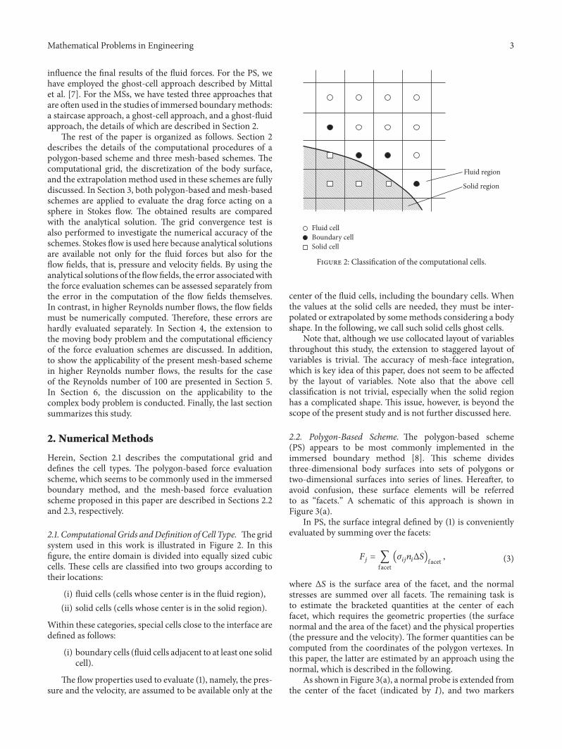
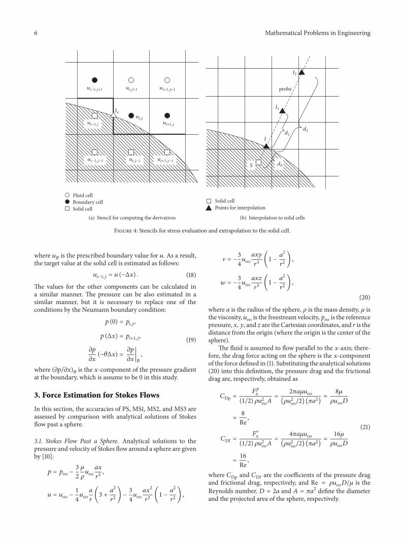
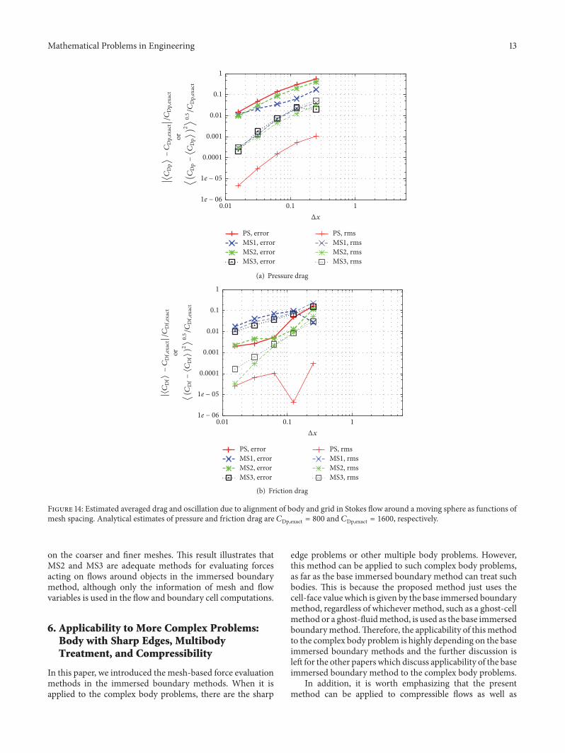(a) Body-conforming grid (b) Nonconforming grid

Figure 1 Examples of body-conforming and nonconforming grids

where120590119894119895 is the stress tensor and 119899119895 is the unit outward normalof the surface element The stress tensor 120590119894119895 of Newtonianfluids is given by

120590119894119895 = minus119901120575119894119895 + 120583(120597119906119895120597119909119894 +

120597119906119894120597119909119895) (2)

where119901 is the pressure 119906119894 is the velocity and120583 is the viscosityIn numerical computations the surface integral defined

by (1) is evaluated in two steps

(i) discretization of the surface(ii) estimation of the physical quantities at the surface

The numerical procedures to conduct these steps depend onthe grid system used in the simulation In body-conformingcurvilinear grid systems shown in Figure 1(a) both steps canbe implemented on the specified grids in a straightforwardmanner However in nonconforming grid systems shownin Figure 1(b) some special treatment is required since thegrids do not exactly match the body surface To the best ofour knowledge there are two different ways which have beenadopted in nonconforming grid systems namely the controlvolume method and the direct calculation

The control volume method introduces a virtual volumewhich encompasses the body and estimates the fluid forcesfrom the net momentum flux through the surface of this vir-tual volume This method was firstly applied to steady forcesby Lai and Peskin [3] and later it was extended to unsteadyforces by Balaras [4] and to moving body problems by Shenet al [5] The control volume method has an advantage thatit is unnecessary to directly handle the complex geometriesexpressed by the immersed boundaries On the other handit has a severe disadvantage that local stresses cannot becomputed that is only the total force acting on the body canbe evaluated Moreover the contributions from pressure andviscous forces cannot be evaluated separately

In the direct calculation the body surface is usuallydiscretized by a set of polygons and the local stresses on these

surface elements are estimated Then the local stresses areintegrated over the body surfaces to obtain the total forceas in body-conforming grid systems However unlike thecases of body-conforming grid systems the estimation of theflow variables on the surface elements is not straightforwardand requires elaborate interpolation andor extrapolationmethods in order to accurately take into account the location(and orientation if necessary) of the surface Moreover thecomputational cost of the stress integration may becomeprohibitive when the body shape is complex since it dependson the number of the polygons used to express the bodysurface Such a dependency is undesirable in particular inengineering applications For example the number of thepolygons reaches up to the order of 107 for an aerodynamicsimulation using a detailed car model with both exterior andinterior parts [6]

In this study we discuss numerical schemes that aresuitable for evaluating fluid forces in nonconforming gridsystems In particular we propose a simple and computa-tionally efficient method for calculating the surface integralin (1) The proposed method is a kind of direct calculationdescribed above Therefore it has inherited an advantageover the control volume method in that the contributionsfrom pressure and viscous forces can be evaluated locally andseparately Moreover in the presentmethod the fluid stressesare integrated over the mesh faces (staircase surfaces) in thegrid system used not over the discretized surface elementsof the original body Therefore the undesirable dependencyon quality or numbers of surface polygons can be removedHereafter the present method is referred to as a ldquomesh-basedscheme (MS)rdquo whereas the method based on the integrationover surface polygons is called a ldquopolygon-based scheme(PS)rdquoWepresent a comparative study of the accuracy of thesemethods

It is worth noting here that in both mesh-based andpolygon-based schemes the physical quantities at the dis-cretized surfaces must be estimated by interpolation orextrapolation and the accuracy of this estimation would




2 Numerical Methods








Fluid region

Solid region






119865119895 = sumfacet

(120590119894119895119899119894Δ119878)facet (3)




Facet

Probe


I2

I1

Id1

d2


Face x

Face yIx

Iy





119901 (119889) = 1198621119889 + 1198620 (4)


119901 (1198891) = 1199011119901 (1198892) = 1199012 (5)




119906 (119889) = 11986221198892 + 1198621119889 + 1198620 (7)


119906 (1198891) = 1199061119906 (1198892) = 1199062119906 (0) = 119906119861

(8)



120597119906120597119899

10038161003816100381610038161003816100381610038161003816119868 =119906111988922 minus 11990621198892111988911198892 (1198892 minus 1198891)

120597119906120597119904

10038161003816100381610038161003816100381610038161003816119868 = 0120597119906120597119905

10038161003816100381610038161003816100381610038161003816119868 = 0

(9)









face119909(120590119909119909119899119909Δ119878)face119909 + sum

face119910(120590119910119909119899119910Δ119878)face119910

+ sumface119911

(120590119911119909119899119911Δ119878)face119911 (10)




119901119868119909 = 119901bc119901119868119910 = 119901bc (11)


120597119906120597119909

10038161003816100381610038161003816100381610038161003816119868119909 =119906119894119895 minus 119906119868Δ1199092

120597119906120597119910

10038161003816100381610038161003816100381610038161003816119868119909 =119906119894119895+1 minus 119906119894119895minus1

2Δ119909 (12)




119901119868119909 = 119901119894119895 + 119901119894minus11198952 (13)


120597119906120597119909

10038161003816100381610038161003816100381610038161003816119868x =119906119894119895 minus 119906119894minus1119895

Δ119909 120597119906120597119910

10038161003816100381610038161003816100381610038161003816119868119909 =12 [119906119894119895+1 minus 119906119894119895minus1


(14)



119901119878 = 119901 (minus1198890) 119906119878 = 119906 (minus1198890) (15)




119891 (119909) = 11986221199092 + 1198621119909 + 1198620 (16)


119906 (0) = 119906119894119895119906 (Δ119909) = 119906119894+1119895

119906 (minus120579Δ119909) = 119906119861(17)



uiminus1j

uijui+1j



Ix


I2

probe

I1

Id1

d2

S d0





119906119894minus1119895 = 119906 (minusΔ119909) (18)


119901 (0) = 119901119894119895119901 (Δ119909) = 119901119894+1119895

120597119901120597119909 (minus120579Δ119909) = 120597119901

12059711990910038161003816100381610038161003816100381610038161003816119861

(19)






1198861199091199033


119886119903 (3 + 1198862

1199032 ) minus 34119906infin

11988611990921199033 (1 minus 1198862

1199032 )


1199032 )


1199032 ) (20)




= 8Re

119862Df = 119865V


= 16Re

(21)





33 Results


1e minus 10

1e minus 08

1e minus 06

00001

001

1

0001 001 01 100001Δx

PSMS1

MS2MS3

C＄ＪminusC

＄ＪＲ＝

Ｎ C

＄ＪＲ＝

Ｎ

(a) Pressure drag

1e minus 05

00001

0001

001

01

1

0001 001 01 100001Δx

PSMS1

MS2MS3

C＄minusC

＄Ｒ

＝Ｎ

C＄Ｒ

＝Ｎ

(b) Friction drag




119862119889119901119909 =intcell 119901119889119910119889119911

(12) 1205881199062infinΔ119910Δ119911119862119889119891119910 =

intcell 120591119909119910 + 120591119910119911119889119909 119889119911(12) 1205881199062infinΔ119909Δ119911

(22)


Line A


minus12

minus06

00

06

12

za

(a) ReferenceLine A

minus12

minus06

00

06

12

za


(b) MS1

Line A

minus12

minus06

00

06

12

za


(c) MS2Line A


minus12

minus06

00

06

12

za

(d) MS3





Line ALine B


minus12

minus06

00

06

12

za

(a) Reference

Line ALine B

minus12

minus06

00

06

12

za


(b) MS1

Line ALine B

minus12

minus06

00

06

12

za


(c) MS2

Line ALine B


minus12

minus06

00

06

12

za

(d) MS3







REFMS1

MS2MS3

0

01

02

03

04

05

06

07

08

CdpxＬＩ

ＨＮC

＄Ｊ















grid





minus02

minus01

0

01

02

03

04

05

06


ReferenceMS1

MS2MS3

Cdf

yＬＩ

ＨＮC

＄

(a) Line A

minus02

minus01

0

01

02

03

04

05

06


ReferenceMS1

MS2MS3

Cdf

yＬＩ

ＨＮC

＄

(b) Line B


0

02

04

06

08

1

12

0001 001 01 100001Δx

MS1MS2


C＄ＪC

＄ＪＲ＝

Ｎ

(a) Pressure drag

0

02

04

06

08

1

12

0001 001 01 100001Δx

MS1MS2


C＄C

＄Ｒ

＝Ｎ

(b) Friction drag







MMExact

001 01 10001Δx

01

012

014

016

018

02

022

024

026

028

03x-

com

pone

nt o

f sur

face

area

vec

tors


MMExact

03

035

04

045

05

055

06

065

07

Surfa

ce ar

ea

001 01 10001Δx

(b) Surface area


08

085

09

095

1

105

11

115

12


PSMS1

MS2MS3

C＄ＪC

＄ＪＲ＝

Ｎ

(a) Pressure drag

08

085

09

095

1

105

11

115

12


PSMS1

MS2MS3

C＄C

＄Ｒ

＝Ｎ

(b) Friction drag








or

001 01 1Δx

1e minus 06

1e minus 05

00001

0001

001

01

1



⟨C

＄Ｊ⟩

minusC

＄ＪＲ＝

Ｎ C

＄ＪＲ

＝Ｎ

⟨(C

＄Ｊminus⟨C

＄Ｊ⟩)

2⟩0

5C

＄ＪＲ＝

Ｎ

(a) Pressure drag

001 01 1Δx

1e minus 06

1e minus 05

00001

0001

001

01

1



or

⟨C＄⟩

minusC

＄Ｒ

＝Ｎ

C＄Ｒ

＝Ｎ

⟨(C

＄minus⟨C

＄⟩)2⟩0

5C

＄Ｒ

＝Ｎ

(b) Friction drag








001 01Δx

PSMS1

MS2MS3

105

106

107

108

109

11

111

112

113

114

115

Dra

g co

effici

ents



7 Conclusions





Nomenclature






Acknowledgments




References


























Volume 2014




Journal of











Journal of


Function Spaces






Algebra





Journal of







2 Numerical Methods








Fluid region

Solid region






119865119895 = sumfacet

(120590119894119895119899119894Δ119878)facet (3)




Facet

Probe


I2

I1

Id1

d2


Face x

Face yIx

Iy





119901 (119889) = 1198621119889 + 1198620 (4)


119901 (1198891) = 1199011119901 (1198892) = 1199012 (5)




119906 (119889) = 11986221198892 + 1198621119889 + 1198620 (7)


119906 (1198891) = 1199061119906 (1198892) = 1199062119906 (0) = 119906119861

(8)



120597119906120597119899

10038161003816100381610038161003816100381610038161003816119868 =119906111988922 minus 11990621198892111988911198892 (1198892 minus 1198891)

120597119906120597119904

10038161003816100381610038161003816100381610038161003816119868 = 0120597119906120597119905

10038161003816100381610038161003816100381610038161003816119868 = 0

(9)









face119909(120590119909119909119899119909Δ119878)face119909 + sum

face119910(120590119910119909119899119910Δ119878)face119910

+ sumface119911

(120590119911119909119899119911Δ119878)face119911 (10)




119901119868119909 = 119901bc119901119868119910 = 119901bc (11)


120597119906120597119909

10038161003816100381610038161003816100381610038161003816119868119909 =119906119894119895 minus 119906119868Δ1199092

120597119906120597119910

10038161003816100381610038161003816100381610038161003816119868119909 =119906119894119895+1 minus 119906119894119895minus1

2Δ119909 (12)




119901119868119909 = 119901119894119895 + 119901119894minus11198952 (13)


120597119906120597119909

10038161003816100381610038161003816100381610038161003816119868x =119906119894119895 minus 119906119894minus1119895

Δ119909 120597119906120597119910

10038161003816100381610038161003816100381610038161003816119868119909 =12 [119906119894119895+1 minus 119906119894119895minus1


(14)



119901119878 = 119901 (minus1198890) 119906119878 = 119906 (minus1198890) (15)




119891 (119909) = 11986221199092 + 1198621119909 + 1198620 (16)


119906 (0) = 119906119894119895119906 (Δ119909) = 119906119894+1119895

119906 (minus120579Δ119909) = 119906119861(17)



uiminus1j

uijui+1j



Ix


I2

probe

I1

Id1

d2

S d0





119906119894minus1119895 = 119906 (minusΔ119909) (18)


119901 (0) = 119901119894119895119901 (Δ119909) = 119901119894+1119895

120597119901120597119909 (minus120579Δ119909) = 120597119901

12059711990910038161003816100381610038161003816100381610038161003816119861

(19)






1198861199091199033


119886119903 (3 + 1198862

1199032 ) minus 34119906infin

11988611990921199033 (1 minus 1198862

1199032 )


1199032 )


1199032 ) (20)




= 8Re

119862Df = 119865V


= 16Re

(21)





33 Results


1e minus 10

1e minus 08

1e minus 06

00001

001

1

0001 001 01 100001Δx

PSMS1

MS2MS3

C＄ＪminusC

＄ＪＲ＝

Ｎ C

＄ＪＲ＝

Ｎ

(a) Pressure drag

1e minus 05

00001

0001

001

01

1

0001 001 01 100001Δx

PSMS1

MS2MS3

C＄minusC

＄Ｒ

＝Ｎ

C＄Ｒ

＝Ｎ

(b) Friction drag




119862119889119901119909 =intcell 119901119889119910119889119911

(12) 1205881199062infinΔ119910Δ119911119862119889119891119910 =

intcell 120591119909119910 + 120591119910119911119889119909 119889119911(12) 1205881199062infinΔ119909Δ119911

(22)


Line A


minus12

minus06

00

06

12

za

(a) ReferenceLine A

minus12

minus06

00

06

12

za


(b) MS1

Line A

minus12

minus06

00

06

12

za


(c) MS2Line A


minus12

minus06

00

06

12

za

(d) MS3





Line ALine B


minus12

minus06

00

06

12

za

(a) Reference

Line ALine B

minus12

minus06

00

06

12

za


(b) MS1

Line ALine B

minus12

minus06

00

06

12

za


(c) MS2

Line ALine B


minus12

minus06

00

06

12

za

(d) MS3







REFMS1

MS2MS3

0

01

02

03

04

05

06

07

08

CdpxＬＩ

ＨＮC

＄Ｊ















grid





minus02

minus01

0

01

02

03

04

05

06


ReferenceMS1

MS2MS3

Cdf

yＬＩ

ＨＮC

＄

(a) Line A

minus02

minus01

0

01

02

03

04

05

06


ReferenceMS1

MS2MS3

Cdf

yＬＩ

ＨＮC

＄

(b) Line B


0

02

04

06

08

1

12

0001 001 01 100001Δx

MS1MS2


C＄ＪC

＄ＪＲ＝

Ｎ

(a) Pressure drag

0

02

04

06

08

1

12

0001 001 01 100001Δx

MS1MS2


C＄C

＄Ｒ

＝Ｎ

(b) Friction drag







MMExact

001 01 10001Δx

01

012

014

016

018

02

022

024

026

028

03x-

com

pone

nt o

f sur

face

area

vec

tors


MMExact

03

035

04

045

05

055

06

065

07

Surfa

ce ar

ea

001 01 10001Δx

(b) Surface area


08

085

09

095

1

105

11

115

12


PSMS1

MS2MS3

C＄ＪC

＄ＪＲ＝

Ｎ

(a) Pressure drag

08

085

09

095

1

105

11

115

12


PSMS1

MS2MS3

C＄C

＄Ｒ

＝Ｎ

(b) Friction drag








or

001 01 1Δx

1e minus 06

1e minus 05

00001

0001

001

01

1



⟨C

＄Ｊ⟩

minusC

＄ＪＲ＝

Ｎ C

＄ＪＲ

＝Ｎ

⟨(C

＄Ｊminus⟨C

＄Ｊ⟩)

2⟩0

5C

＄ＪＲ＝

Ｎ

(a) Pressure drag

001 01 1Δx

1e minus 06

1e minus 05

00001

0001

001

01

1



or

⟨C＄⟩

minusC

＄Ｒ

＝Ｎ

C＄Ｒ

＝Ｎ

⟨(C

＄minus⟨C

＄⟩)2⟩0

5C

＄Ｒ

＝Ｎ

(b) Friction drag








001 01Δx

PSMS1

MS2MS3

105

106

107

108

109

11

111

112

113

114

115

Dra

g co

effici

ents



7 Conclusions





Nomenclature






Acknowledgments




References


























Volume 2014




Journal of











Journal of


Function Spaces






Algebra





Journal of





Facet

Probe


I2

I1

Id1

d2


Face x

Face yIx

Iy





119901 (119889) = 1198621119889 + 1198620 (4)


119901 (1198891) = 1199011119901 (1198892) = 1199012 (5)




119906 (119889) = 11986221198892 + 1198621119889 + 1198620 (7)


119906 (1198891) = 1199061119906 (1198892) = 1199062119906 (0) = 119906119861

(8)



120597119906120597119899

10038161003816100381610038161003816100381610038161003816119868 =119906111988922 minus 11990621198892111988911198892 (1198892 minus 1198891)

120597119906120597119904

10038161003816100381610038161003816100381610038161003816119868 = 0120597119906120597119905

10038161003816100381610038161003816100381610038161003816119868 = 0

(9)









face119909(120590119909119909119899119909Δ119878)face119909 + sum

face119910(120590119910119909119899119910Δ119878)face119910

+ sumface119911

(120590119911119909119899119911Δ119878)face119911 (10)




119901119868119909 = 119901bc119901119868119910 = 119901bc (11)


120597119906120597119909

10038161003816100381610038161003816100381610038161003816119868119909 =119906119894119895 minus 119906119868Δ1199092

120597119906120597119910

10038161003816100381610038161003816100381610038161003816119868119909 =119906119894119895+1 minus 119906119894119895minus1

2Δ119909 (12)




119901119868119909 = 119901119894119895 + 119901119894minus11198952 (13)


120597119906120597119909

10038161003816100381610038161003816100381610038161003816119868x =119906119894119895 minus 119906119894minus1119895

Δ119909 120597119906120597119910

10038161003816100381610038161003816100381610038161003816119868119909 =12 [119906119894119895+1 minus 119906119894119895minus1


(14)



119901119878 = 119901 (minus1198890) 119906119878 = 119906 (minus1198890) (15)




119891 (119909) = 11986221199092 + 1198621119909 + 1198620 (16)


119906 (0) = 119906119894119895119906 (Δ119909) = 119906119894+1119895

119906 (minus120579Δ119909) = 119906119861(17)



uiminus1j

uijui+1j



Ix


I2

probe

I1

Id1

d2

S d0





119906119894minus1119895 = 119906 (minusΔ119909) (18)


119901 (0) = 119901119894119895119901 (Δ119909) = 119901119894+1119895

120597119901120597119909 (minus120579Δ119909) = 120597119901

12059711990910038161003816100381610038161003816100381610038161003816119861

(19)






1198861199091199033


119886119903 (3 + 1198862

1199032 ) minus 34119906infin

11988611990921199033 (1 minus 1198862

1199032 )


1199032 )


1199032 ) (20)




= 8Re

119862Df = 119865V


= 16Re

(21)





33 Results


1e minus 10

1e minus 08

1e minus 06

00001

001

1

0001 001 01 100001Δx

PSMS1

MS2MS3

C＄ＪminusC

＄ＪＲ＝

Ｎ C

＄ＪＲ＝

Ｎ

(a) Pressure drag

1e minus 05

00001

0001

001

01

1

0001 001 01 100001Δx

PSMS1

MS2MS3

C＄minusC

＄Ｒ

＝Ｎ

C＄Ｒ

＝Ｎ

(b) Friction drag




119862119889119901119909 =intcell 119901119889119910119889119911

(12) 1205881199062infinΔ119910Δ119911119862119889119891119910 =

intcell 120591119909119910 + 120591119910119911119889119909 119889119911(12) 1205881199062infinΔ119909Δ119911

(22)


Line A


minus12

minus06

00

06

12

za

(a) ReferenceLine A

minus12

minus06

00

06

12

za


(b) MS1

Line A

minus12

minus06

00

06

12

za


(c) MS2Line A


minus12

minus06

00

06

12

za

(d) MS3





Line ALine B


minus12

minus06

00

06

12

za

(a) Reference

Line ALine B

minus12

minus06

00

06

12

za


(b) MS1

Line ALine B

minus12

minus06

00

06

12

za


(c) MS2

Line ALine B


minus12

minus06

00

06

12

za

(d) MS3







REFMS1

MS2MS3

0

01

02

03

04

05

06

07

08

CdpxＬＩ

ＨＮC

＄Ｊ















grid





minus02

minus01

0

01

02

03

04

05

06


ReferenceMS1

MS2MS3

Cdf

yＬＩ

ＨＮC

＄

(a) Line A

minus02

minus01

0

01

02

03

04

05

06


ReferenceMS1

MS2MS3

Cdf

yＬＩ

ＨＮC

＄

(b) Line B


0

02

04

06

08

1

12

0001 001 01 100001Δx

MS1MS2


C＄ＪC

＄ＪＲ＝

Ｎ

(a) Pressure drag

0

02

04

06

08

1

12

0001 001 01 100001Δx

MS1MS2


C＄C

＄Ｒ

＝Ｎ

(b) Friction drag







MMExact

001 01 10001Δx

01

012

014

016

018

02

022

024

026

028

03x-

com

pone

nt o

f sur

face

area

vec

tors


MMExact

03

035

04

045

05

055

06

065

07

Surfa

ce ar

ea

001 01 10001Δx

(b) Surface area


08

085

09

095

1

105

11

115

12


PSMS1

MS2MS3

C＄ＪC

＄ＪＲ＝

Ｎ

(a) Pressure drag

08

085

09

095

1

105

11

115

12


PSMS1

MS2MS3

C＄C

＄Ｒ

＝Ｎ

(b) Friction drag








or

001 01 1Δx

1e minus 06

1e minus 05

00001

0001

001

01

1



⟨C

＄Ｊ⟩

minusC

＄ＪＲ＝

Ｎ C

＄ＪＲ

＝Ｎ

⟨(C

＄Ｊminus⟨C

＄Ｊ⟩)

2⟩0

5C

＄ＪＲ＝

Ｎ

(a) Pressure drag

001 01 1Δx

1e minus 06

1e minus 05

00001

0001

001

01

1



or

⟨C＄⟩

minusC

＄Ｒ

＝Ｎ

C＄Ｒ

＝Ｎ

⟨(C

＄minus⟨C

＄⟩)2⟩0

5C

＄Ｒ

＝Ｎ

(b) Friction drag








001 01Δx

PSMS1

MS2MS3

105

106

107

108

109

11

111

112

113

114

115

Dra

g co

effici

ents



7 Conclusions





Nomenclature






Acknowledgments




References


























Volume 2014




Journal of











Journal of


Function Spaces






Algebra





Journal of









face119909(120590119909119909119899119909Δ119878)face119909 + sum

face119910(120590119910119909119899119910Δ119878)face119910

+ sumface119911

(120590119911119909119899119911Δ119878)face119911 (10)




119901119868119909 = 119901bc119901119868119910 = 119901bc (11)


120597119906120597119909

10038161003816100381610038161003816100381610038161003816119868119909 =119906119894119895 minus 119906119868Δ1199092

120597119906120597119910

10038161003816100381610038161003816100381610038161003816119868119909 =119906119894119895+1 minus 119906119894119895minus1

2Δ119909 (12)




119901119868119909 = 119901119894119895 + 119901119894minus11198952 (13)


120597119906120597119909

10038161003816100381610038161003816100381610038161003816119868x =119906119894119895 minus 119906119894minus1119895

Δ119909 120597119906120597119910

10038161003816100381610038161003816100381610038161003816119868119909 =12 [119906119894119895+1 minus 119906119894119895minus1


(14)



119901119878 = 119901 (minus1198890) 119906119878 = 119906 (minus1198890) (15)




119891 (119909) = 11986221199092 + 1198621119909 + 1198620 (16)


119906 (0) = 119906119894119895119906 (Δ119909) = 119906119894+1119895

119906 (minus120579Δ119909) = 119906119861(17)



uiminus1j

uijui+1j



Ix


I2

probe

I1

Id1

d2

S d0





119906119894minus1119895 = 119906 (minusΔ119909) (18)


119901 (0) = 119901119894119895119901 (Δ119909) = 119901119894+1119895

120597119901120597119909 (minus120579Δ119909) = 120597119901

12059711990910038161003816100381610038161003816100381610038161003816119861

(19)






1198861199091199033


119886119903 (3 + 1198862

1199032 ) minus 34119906infin

11988611990921199033 (1 minus 1198862

1199032 )


1199032 )


1199032 ) (20)




= 8Re

119862Df = 119865V


= 16Re

(21)





33 Results


1e minus 10

1e minus 08

1e minus 06

00001

001

1

0001 001 01 100001Δx

PSMS1

MS2MS3

C＄ＪminusC

＄ＪＲ＝

Ｎ C

＄ＪＲ＝

Ｎ

(a) Pressure drag

1e minus 05

00001

0001

001

01

1

0001 001 01 100001Δx

PSMS1

MS2MS3

C＄minusC

＄Ｒ

＝Ｎ

C＄Ｒ

＝Ｎ

(b) Friction drag




119862119889119901119909 =intcell 119901119889119910119889119911

(12) 1205881199062infinΔ119910Δ119911119862119889119891119910 =

intcell 120591119909119910 + 120591119910119911119889119909 119889119911(12) 1205881199062infinΔ119909Δ119911

(22)


Line A


minus12

minus06

00

06

12

za

(a) ReferenceLine A

minus12

minus06

00

06

12

za


(b) MS1

Line A

minus12

minus06

00

06

12

za


(c) MS2Line A


minus12

minus06

00

06

12

za

(d) MS3





Line ALine B


minus12

minus06

00

06

12

za

(a) Reference

Line ALine B

minus12

minus06

00

06

12

za


(b) MS1

Line ALine B

minus12

minus06

00

06

12

za


(c) MS2

Line ALine B


minus12

minus06

00

06

12

za

(d) MS3







REFMS1

MS2MS3

0

01

02

03

04

05

06

07

08

CdpxＬＩ

ＨＮC

＄Ｊ















grid





minus02

minus01

0

01

02

03

04

05

06


ReferenceMS1

MS2MS3

Cdf

yＬＩ

ＨＮC

＄

(a) Line A

minus02

minus01

0

01

02

03

04

05

06


ReferenceMS1

MS2MS3

Cdf

yＬＩ

ＨＮC

＄

(b) Line B


0

02

04

06

08

1

12

0001 001 01 100001Δx

MS1MS2


C＄ＪC

＄ＪＲ＝

Ｎ

(a) Pressure drag

0

02

04

06

08

1

12

0001 001 01 100001Δx

MS1MS2


C＄C

＄Ｒ

＝Ｎ

(b) Friction drag







MMExact

001 01 10001Δx

01

012

014

016

018

02

022

024

026

028

03x-

com

pone

nt o

f sur

face

area

vec

tors


MMExact

03

035

04

045

05

055

06

065

07

Surfa

ce ar

ea

001 01 10001Δx

(b) Surface area


08

085

09

095

1

105

11

115

12


PSMS1

MS2MS3

C＄ＪC

＄ＪＲ＝

Ｎ

(a) Pressure drag

08

085

09

095

1

105

11

115

12


PSMS1

MS2MS3

C＄C

＄Ｒ

＝Ｎ

(b) Friction drag








or

001 01 1Δx

1e minus 06

1e minus 05

00001

0001

001

01

1



⟨C

＄Ｊ⟩

minusC

＄ＪＲ＝

Ｎ C

＄ＪＲ

＝Ｎ

⟨(C

＄Ｊminus⟨C

＄Ｊ⟩)

2⟩0

5C

＄ＪＲ＝

Ｎ

(a) Pressure drag

001 01 1Δx

1e minus 06

1e minus 05

00001

0001

001

01

1



or

⟨C＄⟩

minusC

＄Ｒ

＝Ｎ

C＄Ｒ

＝Ｎ

⟨(C

＄minus⟨C

＄⟩)2⟩0

5C

＄Ｒ

＝Ｎ

(b) Friction drag








001 01Δx

PSMS1

MS2MS3

105

106

107

108

109

11

111

112

113

114

115

Dra

g co

effici

ents



7 Conclusions





Nomenclature






Acknowledgments




References


























Volume 2014




Journal of











Journal of


Function Spaces






Algebra





Journal of






uiminus1j

uijui+1j



Ix


I2

probe

I1

Id1

d2

S d0





119906119894minus1119895 = 119906 (minusΔ119909) (18)


119901 (0) = 119901119894119895119901 (Δ119909) = 119901119894+1119895

120597119901120597119909 (minus120579Δ119909) = 120597119901

12059711990910038161003816100381610038161003816100381610038161003816119861

(19)






1198861199091199033


119886119903 (3 + 1198862

1199032 ) minus 34119906infin

11988611990921199033 (1 minus 1198862

1199032 )


1199032 )


1199032 ) (20)




= 8Re

119862Df = 119865V


= 16Re

(21)





33 Results


1e minus 10

1e minus 08

1e minus 06

00001

001

1

0001 001 01 100001Δx

PSMS1

MS2MS3

C＄ＪminusC

＄ＪＲ＝

Ｎ C

＄ＪＲ＝

Ｎ

(a) Pressure drag

1e minus 05

00001

0001

001

01

1

0001 001 01 100001Δx

PSMS1

MS2MS3

C＄minusC

＄Ｒ

＝Ｎ

C＄Ｒ

＝Ｎ

(b) Friction drag




119862119889119901119909 =intcell 119901119889119910119889119911

(12) 1205881199062infinΔ119910Δ119911119862119889119891119910 =

intcell 120591119909119910 + 120591119910119911119889119909 119889119911(12) 1205881199062infinΔ119909Δ119911

(22)


Line A


minus12

minus06

00

06

12

za

(a) ReferenceLine A

minus12

minus06

00

06

12

za


(b) MS1

Line A

minus12

minus06

00

06

12

za


(c) MS2Line A


minus12

minus06

00

06

12

za

(d) MS3





Line ALine B


minus12

minus06

00

06

12

za

(a) Reference

Line ALine B

minus12

minus06

00

06

12

za


(b) MS1

Line ALine B

minus12

minus06

00

06

12

za


(c) MS2

Line ALine B


minus12

minus06

00

06

12

za

(d) MS3







REFMS1

MS2MS3

0

01

02

03

04

05

06

07

08

CdpxＬＩ

ＨＮC

＄Ｊ















grid





minus02

minus01

0

01

02

03

04

05

06


ReferenceMS1

MS2MS3

Cdf

yＬＩ

ＨＮC

＄

(a) Line A

minus02

minus01

0

01

02

03

04

05

06


ReferenceMS1

MS2MS3

Cdf

yＬＩ

ＨＮC

＄

(b) Line B


0

02

04

06

08

1

12

0001 001 01 100001Δx

MS1MS2


C＄ＪC

＄ＪＲ＝

Ｎ

(a) Pressure drag

0

02

04

06

08

1

12

0001 001 01 100001Δx

MS1MS2


C＄C

＄Ｒ

＝Ｎ

(b) Friction drag







MMExact

001 01 10001Δx

01

012

014

016

018

02

022

024

026

028

03x-

com

pone

nt o

f sur

face

area

vec

tors


MMExact

03

035

04

045

05

055

06

065

07

Surfa

ce ar

ea

001 01 10001Δx

(b) Surface area


08

085

09

095

1

105

11

115

12


PSMS1

MS2MS3

C＄ＪC

＄ＪＲ＝

Ｎ

(a) Pressure drag

08

085

09

095

1

105

11

115

12


PSMS1

MS2MS3

C＄C

＄Ｒ

＝Ｎ

(b) Friction drag








or

001 01 1Δx

1e minus 06

1e minus 05

00001

0001

001

01

1



⟨C

＄Ｊ⟩

minusC

＄ＪＲ＝

Ｎ C

＄ＪＲ

＝Ｎ

⟨(C

＄Ｊminus⟨C

＄Ｊ⟩)

2⟩0

5C

＄ＪＲ＝

Ｎ

(a) Pressure drag

001 01 1Δx

1e minus 06

1e minus 05

00001

0001

001

01

1



or

⟨C＄⟩

minusC

＄Ｒ

＝Ｎ

C＄Ｒ

＝Ｎ

⟨(C

＄minus⟨C

＄⟩)2⟩0

5C

＄Ｒ

＝Ｎ

(b) Friction drag








001 01Δx

PSMS1

MS2MS3

105

106

107

108

109

11

111

112

113

114

115

Dra

g co

effici

ents



7 Conclusions





Nomenclature






Acknowledgments




References


























Volume 2014




Journal of











Journal of


Function Spaces






Algebra





Journal of







33 Results


1e minus 10

1e minus 08

1e minus 06

00001

001

1

0001 001 01 100001Δx

PSMS1

MS2MS3

C＄ＪminusC

＄ＪＲ＝

Ｎ C

＄ＪＲ＝

Ｎ

(a) Pressure drag

1e minus 05

00001

0001

001

01

1

0001 001 01 100001Δx

PSMS1

MS2MS3

C＄minusC

＄Ｒ

＝Ｎ

C＄Ｒ

＝Ｎ

(b) Friction drag




119862119889119901119909 =intcell 119901119889119910119889119911

(12) 1205881199062infinΔ119910Δ119911119862119889119891119910 =

intcell 120591119909119910 + 120591119910119911119889119909 119889119911(12) 1205881199062infinΔ119909Δ119911

(22)


Line A


minus12

minus06

00

06

12

za

(a) ReferenceLine A

minus12

minus06

00

06

12

za


(b) MS1

Line A

minus12

minus06

00

06

12

za


(c) MS2Line A


minus12

minus06

00

06

12

za

(d) MS3





Line ALine B


minus12

minus06

00

06

12

za

(a) Reference

Line ALine B

minus12

minus06

00

06

12

za


(b) MS1

Line ALine B

minus12

minus06

00

06

12

za


(c) MS2

Line ALine B


minus12

minus06

00

06

12

za

(d) MS3







REFMS1

MS2MS3

0

01

02

03

04

05

06

07

08

CdpxＬＩ

ＨＮC

＄Ｊ















grid





minus02

minus01

0

01

02

03

04

05

06


ReferenceMS1

MS2MS3

Cdf

yＬＩ

ＨＮC

＄

(a) Line A

minus02

minus01

0

01

02

03

04

05

06


ReferenceMS1

MS2MS3

Cdf

yＬＩ

ＨＮC

＄

(b) Line B


0

02

04

06

08

1

12

0001 001 01 100001Δx

MS1MS2


C＄ＪC

＄ＪＲ＝

Ｎ

(a) Pressure drag

0

02

04

06

08

1

12

0001 001 01 100001Δx

MS1MS2


C＄C

＄Ｒ

＝Ｎ

(b) Friction drag







MMExact

001 01 10001Δx

01

012

014

016

018

02

022

024

026

028

03x-

com

pone

nt o

f sur

face

area

vec

tors


MMExact

03

035

04

045

05

055

06

065

07

Surfa

ce ar

ea

001 01 10001Δx

(b) Surface area


08

085

09

095

1

105

11

115

12


PSMS1

MS2MS3

C＄ＪC

＄ＪＲ＝

Ｎ

(a) Pressure drag

08

085

09

095

1

105

11

115

12


PSMS1

MS2MS3

C＄C

＄Ｒ

＝Ｎ

(b) Friction drag








or

001 01 1Δx

1e minus 06

1e minus 05

00001

0001

001

01

1



⟨C

＄Ｊ⟩

minusC

＄ＪＲ＝

Ｎ C

＄ＪＲ

＝Ｎ

⟨(C

＄Ｊminus⟨C

＄Ｊ⟩)

2⟩0

5C

＄ＪＲ＝

Ｎ

(a) Pressure drag

001 01 1Δx

1e minus 06

1e minus 05

00001

0001

001

01

1



or

⟨C＄⟩

minusC

＄Ｒ

＝Ｎ

C＄Ｒ

＝Ｎ

⟨(C

＄minus⟨C

＄⟩)2⟩0

5C

＄Ｒ

＝Ｎ

(b) Friction drag








001 01Δx

PSMS1

MS2MS3

105

106

107

108

109

11

111

112

113

114

115

Dra

g co

effici

ents



7 Conclusions





Nomenclature






Acknowledgments




References


























Volume 2014




Journal of











Journal of


Function Spaces






Algebra





Journal of





Line A


minus12

minus06

00

06

12

za

(a) ReferenceLine A

minus12

minus06

00

06

12

za


(b) MS1

Line A

minus12

minus06

00

06

12

za


(c) MS2Line A


minus12

minus06

00

06

12

za

(d) MS3





Line ALine B


minus12

minus06

00

06

12

za

(a) Reference

Line ALine B

minus12

minus06

00

06

12

za


(b) MS1

Line ALine B

minus12

minus06

00

06

12

za


(c) MS2

Line ALine B


minus12

minus06

00

06

12

za

(d) MS3







REFMS1

MS2MS3

0

01

02

03

04

05

06

07

08

CdpxＬＩ

ＨＮC

＄Ｊ















grid





minus02

minus01

0

01

02

03

04

05

06


ReferenceMS1

MS2MS3

Cdf

yＬＩ

ＨＮC

＄

(a) Line A

minus02

minus01

0

01

02

03

04

05

06


ReferenceMS1

MS2MS3

Cdf

yＬＩ

ＨＮC

＄

(b) Line B


0

02

04

06

08

1

12

0001 001 01 100001Δx

MS1MS2


C＄ＪC

＄ＪＲ＝

Ｎ

(a) Pressure drag

0

02

04

06

08

1

12

0001 001 01 100001Δx

MS1MS2


C＄C

＄Ｒ

＝Ｎ

(b) Friction drag







MMExact

001 01 10001Δx

01

012

014

016

018

02

022

024

026

028

03x-

com

pone

nt o

f sur

face

area

vec

tors


MMExact

03

035

04

045

05

055

06

065

07

Surfa

ce ar

ea

001 01 10001Δx

(b) Surface area


08

085

09

095

1

105

11

115

12


PSMS1

MS2MS3

C＄ＪC

＄ＪＲ＝

Ｎ

(a) Pressure drag

08

085

09

095

1

105

11

115

12


PSMS1

MS2MS3

C＄C

＄Ｒ

＝Ｎ

(b) Friction drag








or

001 01 1Δx

1e minus 06

1e minus 05

00001

0001

001

01

1



⟨C

＄Ｊ⟩

minusC

＄ＪＲ＝

Ｎ C

＄ＪＲ

＝Ｎ

⟨(C

＄Ｊminus⟨C

＄Ｊ⟩)

2⟩0

5C

＄ＪＲ＝

Ｎ

(a) Pressure drag

001 01 1Δx

1e minus 06

1e minus 05

00001

0001

001

01

1



or

⟨C＄⟩

minusC

＄Ｒ

＝Ｎ

C＄Ｒ

＝Ｎ

⟨(C

＄minus⟨C

＄⟩)2⟩0

5C

＄Ｒ

＝Ｎ

(b) Friction drag








001 01Δx

PSMS1

MS2MS3

105

106

107

108

109

11

111

112

113

114

115

Dra

g co

effici

ents



7 Conclusions





Nomenclature






Acknowledgments




References


























Volume 2014




Journal of











Journal of


Function Spaces






Algebra





Journal of





Line ALine B


minus12

minus06

00

06

12

za

(a) Reference

Line ALine B

minus12

minus06

00

06

12

za


(b) MS1

Line ALine B

minus12

minus06

00

06

12

za


(c) MS2

Line ALine B


minus12

minus06

00

06

12

za

(d) MS3







REFMS1

MS2MS3

0

01

02

03

04

05

06

07

08

CdpxＬＩ

ＨＮC

＄Ｊ















grid





minus02

minus01

0

01

02

03

04

05

06


ReferenceMS1

MS2MS3

Cdf

yＬＩ

ＨＮC

＄

(a) Line A

minus02

minus01

0

01

02

03

04

05

06


ReferenceMS1

MS2MS3

Cdf

yＬＩ

ＨＮC

＄

(b) Line B


0

02

04

06

08

1

12

0001 001 01 100001Δx

MS1MS2


C＄ＪC

＄ＪＲ＝

Ｎ

(a) Pressure drag

0

02

04

06

08

1

12

0001 001 01 100001Δx

MS1MS2


C＄C

＄Ｒ

＝Ｎ

(b) Friction drag







MMExact

001 01 10001Δx

01

012

014

016

018

02

022

024

026

028

03x-

com

pone

nt o

f sur

face

area

vec

tors


MMExact

03

035

04

045

05

055

06

065

07

Surfa

ce ar

ea

001 01 10001Δx

(b) Surface area


08

085

09

095

1

105

11

115

12


PSMS1

MS2MS3

C＄ＪC

＄ＪＲ＝

Ｎ

(a) Pressure drag

08

085

09

095

1

105

11

115

12


PSMS1

MS2MS3

C＄C

＄Ｒ

＝Ｎ

(b) Friction drag








or

001 01 1Δx

1e minus 06

1e minus 05

00001

0001

001

01

1



⟨C

＄Ｊ⟩

minusC

＄ＪＲ＝

Ｎ C

＄ＪＲ

＝Ｎ

⟨(C

＄Ｊminus⟨C

＄Ｊ⟩)

2⟩0

5C

＄ＪＲ＝

Ｎ

(a) Pressure drag

001 01 1Δx

1e minus 06

1e minus 05

00001

0001

001

01

1



or

⟨C＄⟩

minusC

＄Ｒ

＝Ｎ

C＄Ｒ

＝Ｎ

⟨(C

＄minus⟨C

＄⟩)2⟩0

5C

＄Ｒ

＝Ｎ

(b) Friction drag








001 01Δx

PSMS1

MS2MS3

105

106

107

108

109

11

111

112

113

114

115

Dra

g co

effici

ents



7 Conclusions





Nomenclature






Acknowledgments




References


























Volume 2014




Journal of











Journal of


Function Spaces






Algebra





Journal of






REFMS1

MS2MS3

0

01

02

03

04

05

06

07

08

CdpxＬＩ

ＨＮC

＄Ｊ















grid





minus02

minus01

0

01

02

03

04

05

06


ReferenceMS1

MS2MS3

Cdf

yＬＩ

ＨＮC

＄

(a) Line A

minus02

minus01

0

01

02

03

04

05

06


ReferenceMS1

MS2MS3

Cdf

yＬＩ

ＨＮC

＄

(b) Line B


0

02

04

06

08

1

12

0001 001 01 100001Δx

MS1MS2


C＄ＪC

＄ＪＲ＝

Ｎ

(a) Pressure drag

0

02

04

06

08

1

12

0001 001 01 100001Δx

MS1MS2


C＄C

＄Ｒ

＝Ｎ

(b) Friction drag







MMExact

001 01 10001Δx

01

012

014

016

018

02

022

024

026

028

03x-

com

pone

nt o

f sur

face

area

vec

tors


MMExact

03

035

04

045

05

055

06

065

07

Surfa

ce ar

ea

001 01 10001Δx

(b) Surface area


08

085

09

095

1

105

11

115

12


PSMS1

MS2MS3

C＄ＪC

＄ＪＲ＝

Ｎ

(a) Pressure drag

08

085

09

095

1

105

11

115

12


PSMS1

MS2MS3

C＄C

＄Ｒ

＝Ｎ

(b) Friction drag








or

001 01 1Δx

1e minus 06

1e minus 05

00001

0001

001

01

1



⟨C

＄Ｊ⟩

minusC

＄ＪＲ＝

Ｎ C

＄ＪＲ

＝Ｎ

⟨(C

＄Ｊminus⟨C

＄Ｊ⟩)

2⟩0

5C

＄ＪＲ＝

Ｎ

(a) Pressure drag

001 01 1Δx

1e minus 06

1e minus 05

00001

0001

001

01

1



or

⟨C＄⟩

minusC

＄Ｒ

＝Ｎ

C＄Ｒ

＝Ｎ

⟨(C

＄minus⟨C

＄⟩)2⟩0

5C

＄Ｒ

＝Ｎ

(b) Friction drag








001 01Δx

PSMS1

MS2MS3

105

106

107

108

109

11

111

112

113

114

115

Dra

g co

effici

ents



7 Conclusions





Nomenclature






Acknowledgments




References


























Volume 2014




Journal of











Journal of


Function Spaces






Algebra





Journal of





minus02

minus01

0

01

02

03

04

05

06


ReferenceMS1

MS2MS3

Cdf

yＬＩ

ＨＮC

＄

(a) Line A

minus02

minus01

0

01

02

03

04

05

06


ReferenceMS1

MS2MS3

Cdf

yＬＩ

ＨＮC

＄

(b) Line B


0

02

04

06

08

1

12

0001 001 01 100001Δx

MS1MS2


C＄ＪC

＄ＪＲ＝

Ｎ

(a) Pressure drag

0

02

04

06

08

1

12

0001 001 01 100001Δx

MS1MS2


C＄C

＄Ｒ

＝Ｎ

(b) Friction drag







MMExact

001 01 10001Δx

01

012

014

016

018

02

022

024

026

028

03x-

com

pone

nt o

f sur

face

area

vec

tors


MMExact

03

035

04

045

05

055

06

065

07

Surfa

ce ar

ea

001 01 10001Δx

(b) Surface area


08

085

09

095

1

105

11

115

12


PSMS1

MS2MS3

C＄ＪC

＄ＪＲ＝

Ｎ

(a) Pressure drag

08

085

09

095

1

105

11

115

12


PSMS1

MS2MS3

C＄C

＄Ｒ

＝Ｎ

(b) Friction drag








or

001 01 1Δx

1e minus 06

1e minus 05

00001

0001

001

01

1



⟨C

＄Ｊ⟩

minusC

＄ＪＲ＝

Ｎ C

＄ＪＲ

＝Ｎ

⟨(C

＄Ｊminus⟨C

＄Ｊ⟩)

2⟩0

5C

＄ＪＲ＝

Ｎ

(a) Pressure drag

001 01 1Δx

1e minus 06

1e minus 05

00001

0001

001

01

1



or

⟨C＄⟩

minusC

＄Ｒ

＝Ｎ

C＄Ｒ

＝Ｎ

⟨(C

＄minus⟨C

＄⟩)2⟩0

5C

＄Ｒ

＝Ｎ

(b) Friction drag








001 01Δx

PSMS1

MS2MS3

105

106

107

108

109

11

111

112

113

114

115

Dra

g co

effici

ents



7 Conclusions





Nomenclature






Acknowledgments




References


























Volume 2014




Journal of











Journal of


Function Spaces






Algebra





Journal of





MMExact

001 01 10001Δx

01

012

014

016

018

02

022

024

026

028

03x-

com

pone

nt o

f sur

face

area

vec

tors


MMExact

03

035

04

045

05

055

06

065

07

Surfa

ce ar

ea

001 01 10001Δx

(b) Surface area


08

085

09

095

1

105

11

115

12


PSMS1

MS2MS3

C＄ＪC

＄ＪＲ＝

Ｎ

(a) Pressure drag

08

085

09

095

1

105

11

115

12


PSMS1

MS2MS3

C＄C

＄Ｒ

＝Ｎ

(b) Friction drag








or

001 01 1Δx

1e minus 06

1e minus 05

00001

0001

001

01

1



⟨C

＄Ｊ⟩

minusC

＄ＪＲ＝

Ｎ C

＄ＪＲ

＝Ｎ

⟨(C

＄Ｊminus⟨C

＄Ｊ⟩)

2⟩0

5C

＄ＪＲ＝

Ｎ

(a) Pressure drag

001 01 1Δx

1e minus 06

1e minus 05

00001

0001

001

01

1



or

⟨C＄⟩

minusC

＄Ｒ

＝Ｎ

C＄Ｒ

＝Ｎ

⟨(C

＄minus⟨C

＄⟩)2⟩0

5C

＄Ｒ

＝Ｎ

(b) Friction drag








001 01Δx

PSMS1

MS2MS3

105

106

107

108

109

11

111

112

113

114

115

Dra

g co

effici

ents



7 Conclusions





Nomenclature






Acknowledgments




References


























Volume 2014




Journal of











Journal of


Function Spaces






Algebra





Journal of





or

001 01 1Δx

1e minus 06

1e minus 05

00001

0001

001

01

1



⟨C

＄Ｊ⟩

minusC

＄ＪＲ＝

Ｎ C

＄ＪＲ

＝Ｎ

⟨(C

＄Ｊminus⟨C

＄Ｊ⟩)

2⟩0

5C

＄ＪＲ＝

Ｎ

(a) Pressure drag

001 01 1Δx

1e minus 06

1e minus 05

00001

0001

001

01

1



or

⟨C＄⟩

minusC

＄Ｒ

＝Ｎ

C＄Ｒ

＝Ｎ

⟨(C

＄minus⟨C

＄⟩)2⟩0

5C

＄Ｒ

＝Ｎ

(b) Friction drag








001 01Δx

PSMS1

MS2MS3

105

106

107

108

109

11

111

112

113

114

115

Dra

g co

effici

ents



7 Conclusions





Nomenclature






Acknowledgments




References


























Volume 2014




Journal of











Journal of


Function Spaces






Algebra





Journal of





001 01Δx

PSMS1

MS2MS3

105

106

107

108

109

11

111

112

113

114

115

Dra

g co

effici

ents



7 Conclusions





Nomenclature






Acknowledgments




References


























Volume 2014




Journal of











Journal of


Function Spaces






Algebra





Journal of






References


























Volume 2014




Journal of











Journal of


Function Spaces






Algebra





Journal of











Volume 2014




Journal of











Journal of


Function Spaces






Algebra





Journal of




a comparative study on evaluation methods of fluid forces

Documents