a comparative study of various inclusive indices and the index constructed by the principal...
TRANSCRIPT
8/14/2019 A Comparative Study of Various Inclusive Indices and the Index Constructed by the Principal Components Analysis
http://slidepdf.com/reader/full/a-comparative-study-of-various-inclusive-indices-and-the-index-constructed 1/14
A Comparative Study of Various Inclusive Indices and
the Index Constructed by the Principal Components Analysis
SK Mishra
Department of Economics
North-Eastern Hill University
Shillong (India)
Introduction: A composite index (or simply an index) is constructed with an objective to
obtain a synoptic or comprehensive single number, representing a vast array of measurements
on the multiple aspects of a ‘conceptual entity’ such as general price level, cost of living, levelof economic development and regional disparities (Adelman and Morris, 1967; Pal, 1975;
Mishra and Chopra, 1978; Mishra and Gaikwad, 1979), quality of life (Mishra and Ngullie,
2003), human development (Cahill and Sánchez, 2001; OECD, 2003; Jahan, 2005), status of social well being (Salzman, 2003), etc. Following Saltelli (2007), Michalos et al. (2006),
Nardo, et al. (2005), Booysen (2002) and Michalos (1980) the list of advantages of composite
indices (enlisted by Michalos et al. 2006) may me presented as follows:
A single composite index yielding a single numerical value is an excellent communications tool
for use with practically any constituency, including the news media, general public, and elected
and un-elected key decision-makers
Such indices provide simple targets facilitating the focus of attention
The simplicity of a composite index facilitates necessary negotiations about its practical value
and usefulness
Reduced transaction costs of negotiations with such indicators increase the latter’s efficiency
and effectiveness, probably leading to the development of better policies and programs
Such indices provide a means to simplifying complex, multi-dimensional phenomena and
measures
They make it easier to measure and visually represent overall trends in several distinct
indicators over time and/or across geographic regions Increase in the ease of measuring and representing trends increases our ability to predict and
possibly manage future trends
They provide a means of comparing diverse phenomena and assessing their relative
importance, status or standing on the basis of some common scale of measurement, across time
and space.
Such composite indices are often a weighted linear combination of a host of variables
that may be symbolically expressed as I=Xw, where X is an n m× matrix of measurements in n
rows (cases) and m columns (variables), w is a column vector of m elements and, therefore, I
is a column vector of n index values, one for each case, summarizing all variables for the case
concerned. Alternatively, it may be expressed as
1 1 2 2
1
... ; 1,2,...,m
i j ij i i m im
j
I w x w x w x w x i n=
= = + + + =∑
There are two approaches to determining w or weights; first by assessing theimportance of different variables with regard to the entity, idea or concept that they measure
(Munda and Nardo, 2005) and secondly by obtaining those weights intrinsically. In the first
case the weights are obtained from extraneous information. They might be based on the expert
8/14/2019 A Comparative Study of Various Inclusive Indices and the Index Constructed by the Principal Components Analysis
http://slidepdf.com/reader/full/a-comparative-study-of-various-inclusive-indices-and-the-index-constructed 2/14
2
opinion or some other data, say, Y. However, in the second case, weights are derived (on sometheoretical considerations - often mathematical) from the data (X) itself.
The Principal Components Analysis (PCA) is perhaps the most-used method to obtain
weights intrinsically. The PCA determines weights of different variables such that the sum of
the squared coefficients of (the product moment) correlation between the index ( I ) and thevariables (X) is maximized. If we denote by r(I, x j) the coefficient of correlation between I and
x j, then the PCA weights are obtained such that 2
1( , )
m
j jr I x
=∑ is maximized.
The PCA has excellent mathematically desirable properties (Kendall and Stuart, 1968).
Among those, the most important property is that the index so obtained relates to the firstprincipal component, which explains the largest part of variation in the constituent variables
(X). Secondly, from the residual, one may obtain the subsequent indices that are orthogonal to
the first index (as well as to other indices so derived). These indices together explain the
variations in the data (X) completely.
However, the PCA has only one objective: to construct an orthogonal index thatexplains the largest portion of variation in the constituent variables. This is obtained bymaximizing the sum of the squared coefficient of correlation coefficients between the index ( I )
and the variables (X). In so doing, the PCA is not concerned with the question as to which
particular variables obtain large or small weights, or which variables are only poorlyrepresented by the index, etc. As a result what happens in practice is that when a group of
variables is poorly correlated with others in the entire data set, the PCA index assigns very
small loadings to some and larger loadings to the other variables if such loadings help in
maximizing the sum of the squared correlation coefficients between the index ( I ) and thevariables (X). Consequently, PCA loadings are highly elitist – preferring highly correlated
variables to poorly correlated variables, irrespective of the (possible) contextual importance of
the latter set of variables. On many occasions it is found that some (evidently) very importantvariables are roughly dealt with by the PCA simply because those variables exhibited widely
distributed scatter or they failed to fall within a narrow band around a straight line. Further,
although the PCA may permit construction of the subsequent indices (orthogonal to the firstleading index), it may not be possible to use them for any comprehensive analysis since there is
no dependable procedure to make an index by merging several principal component indices
derived from the data (X).
It is not unusual, therefore, that the PCA performs poorly at constructing
comprehensive indices from the variables especially if the data pertain to a system that has not
evolved sufficiently (fully) such that everything determines everything else (and thus the
variables drawn from the system are highly inter-correlated). It is well known thatunderdeveloped economies characterize underdeveloped intra-systemic interdependence as
well as underdeveloped data recording mechanism. Therefore, variables drawn from anunderdeveloped system exhibit widely distributed scatters and poor inter-correlations among
different measurements. The elitist approach of the PCA therefore does not suit to the
underdeveloped systems.
8/14/2019 A Comparative Study of Various Inclusive Indices and the Index Constructed by the Principal Components Analysis
http://slidepdf.com/reader/full/a-comparative-study-of-various-inclusive-indices-and-the-index-constructed 3/14
3
Apart from this, data may contain outliers. Those outliers may pull down (or up)correlation coefficients of the one set of variables with the rest others and thus affect the index
unpredictably. The variables favored or disfavored by the PCA may obtain entirely
unwarranted weights. It could have been proper in such condition to use the absolute analog of
the product moment correlation coefficient suggested by Bradley (1985) who showed that if
( , ), 1, 2, ...,i iu v i n=
are n pairs of values such that the variables u and v have the same0median = and the same mean deviation (from median),
1 1(1 / ) (1/ )
n n
i ii in u n v
= =
=∑ ∑ , both of
which conditions may be met by any pair of variables when suitably transformed, the absolute
correlation may then be defined as1 1
( , ) { } / { }n n
i i i i i ii iu v u v u v u v ρ
= =
= + − − +∑ ∑ that lies between
[ 1, 1]− . However, it is a moot question whether the PCA can be carried out (perhaps not!) on
the inter-correlation matrices containing a row (column) of absolute correlation coefficients
while the other rows (columns) contain the product moment correlation coefficients.
Alternative Methods for Deriving Objective Weights: To draw more attention to the
representation of each variable correlated strongly or weakly with the other fellow variables in
the data to be used for construction of an index, albeit with some compromise on theexplanatory power of the index regarding variation in the data (X), Mishra (2007) proposed
two methods. The first, (I1), maximizes the sum of absolute correlation coefficients of the
index with the constituent variables and the second, (IM), maximizes the minimal correlationcoefficient of the index with the constituent variables. It was shown that I1 improves the
representation of weakly correlated variables while IM has a tendency to be almost equally
correlated with most of the constituent variables in which the weakly correlated variables have
a secure representation. These two types of index were called ‘inclusive’ and ‘egalitarian’respectively. It was also shown that the inclusive index (I1) has an explanatory power only
slightly less than the PCA index (I2), which is clearly due to a trade-off between individual
representation and overall representation or explanatory power. However, the egalitarian index
(IM) has much larger trade-off.
The Objectives of this Paper: In this paper we further inquire if inclusive indices (I1)improve the representation of weakly correlated variables while the egalitarian indices (IM) are
almost equally correlated with most of the constituent variables. We also introduce a new index
that, in some sense, maximizes an analogue of entropy in the data used for constructing the
index. If we define1
( , ) ; ( , ) / , 1, 2, ...,m
j j j j B r I x b r I x B j m
=
= = =∑ where ( , ) j
r I x =coefficient of
correlation between the index (I) and the constituent variable j x , an index may be constructed
so as to maximizes1[ ln( )] ln( )
m
j j jb b B B
=
+∑ . We will call such an index IE.
The Computational Aspects: For obtaining the PCA indices one may apply the usualprocedure (available in many software packages such as STATISTICA or SPSS). The procedure
runs as follows. First, the (product moment) correlation matrix,m m
R×
is obtained from the data
on X =(x1, x2,…,xm). Then the largest (first) eigenvalue (λ ) and the associated eigenvector ( v )
of R are obtained and the eigenvector is standardized such that its squared Euclidean norm is
equal to the eigenvalue. This standardized eigenvector (call it *v ) is used to obtain * *
2 I X v= ,
where * X is obtained from X such that each variable has zero mean and unit standard
8/14/2019 A Comparative Study of Various Inclusive Indices and the Index Constructed by the Principal Components Analysis
http://slidepdf.com/reader/full/a-comparative-study-of-various-inclusive-indices-and-the-index-constructed 4/14
4
deviation. In some cases, however, the eigenvector is standardized such that its Euclidean normis equal to unity. These alternative schemes of standardization of the eigenvector only differ as
to the scale of the index (I2), but its correlation coefficients with the constituent variables
remain unaltered. If one desires, the index can have non-zero mean as well and this can be
done by a suitable transformation of the zero-mean index (I2), without any effect on its
correlation structure.
Alternatively, one may maximize 2
2 21( , );
m
j jr I x I Xw
=
=∑ directly, without going through
the matrix operations detailed out above. It requires solving the nonlinear programming
problem straight away using1 2
( , ,..., )m
w w w w= as the vector of decision variables. Although
this direct optimization method has seldom been used to construct an index, it has flexibility
and generality while the matrix method is specific but (possibly) simpler.
The flexibility of the direct optimization method is very handy when we need I1, IM orIE type of index. We obtain
2
I Xw= by maximization of 2
21
( , )m
j j
r I x=
∑
1 I Xw= by maximization of
11( , )
m
j jr I x
=∑
M I Xw= by maximization of ( )min ( , )
M j j
r I x
E I Xw= by maximization of
1 1[ ln( )] ln( ) : ( , ) ; ( , ) / , 1, 2, ...,
m m
j j j j j j jb b B B B r I x b r I x B j m
= =
+ = = =∑ ∑
We have optimized the functions by direct non-linear programming for which we usethe Differential Evolution method (Mishra, 2006-a). Particle Swarm optimization (Mishra,
2006-b) also yields equally good results (not presented here to avoid duplication).
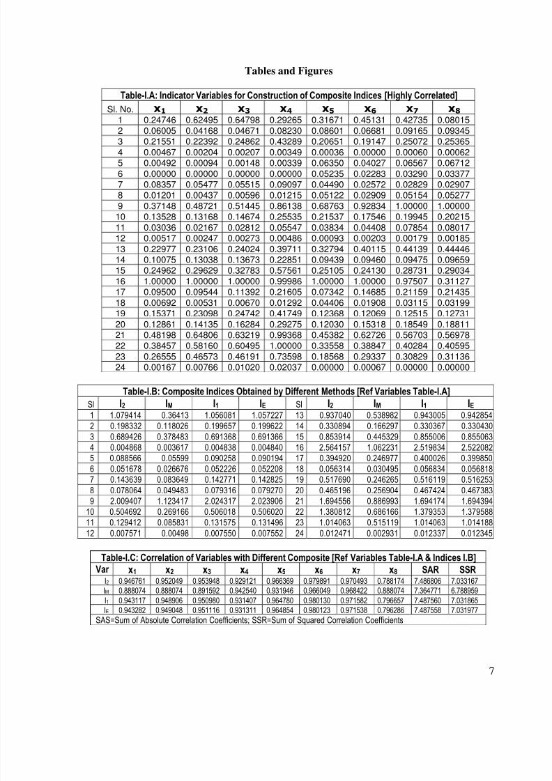
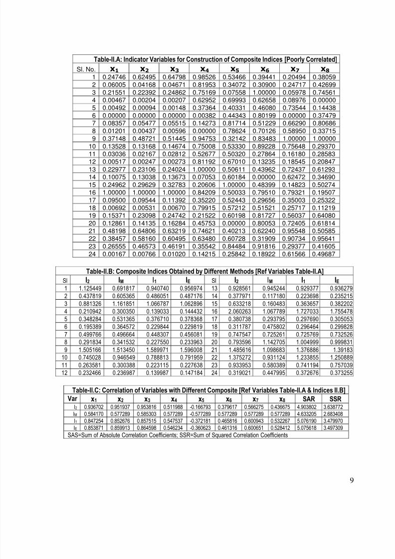
The Main Findings: We have used four sets of eight variables to construct indices. Amongthese sets, the first has the variables that correlate highly among themselves (Table-I.A). The
other three sets contain some variables that correlate highly with some of their fellow variables,but they correlate only poorly with the others (Tables II.A through IV.A). All the four indices
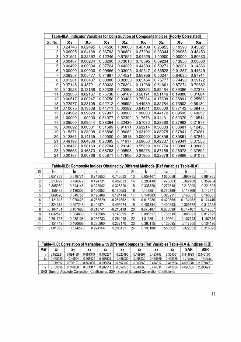
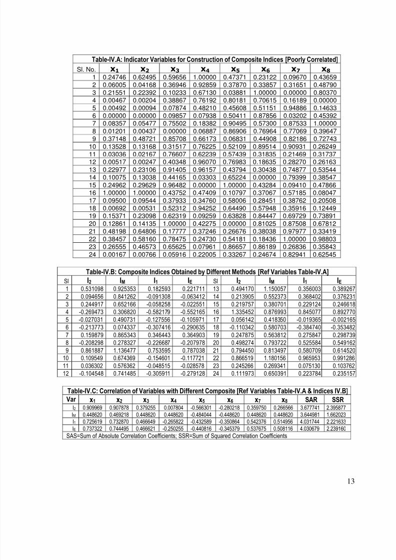
are obtained for each set of data. These indices are presented in Tables-I.B, II.B, III.B and
IV.B. Their correlation coefficients with the constituent variables, the SAR (sum of absolute
correlation coefficients) and SSR (sum of squared correlation coefficients) are presented inTables-I.C, II.C, III.C and IV.C. The correlation coefficients among the constituent variables,
among different indices, as well as across the indices and the constituent variables are
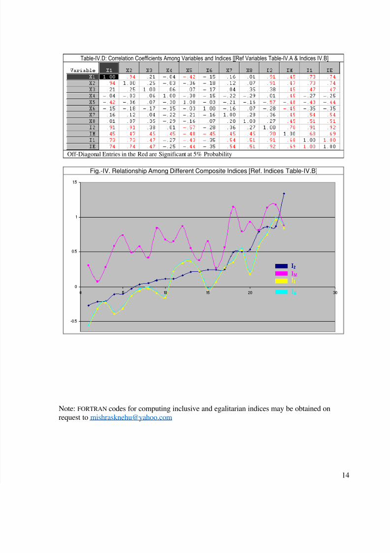
presented in Tables I.D, II.D, III.D and IV.D. Different indices for each set of data have beengraphically presented in Fig.-I through Fig.-IV. All indices are ordered in conformity with the
ascending order of values of I2 (the PCA index) to facilitate comparison. Instead of presentingthe indices as points associated with each case (from 1 to 24), which is more appropriate,curves have been drawn only to facilitate comprehension visually.
First, we find that when all the variables are highly correlated among themselves, I2, I1
and IE are very close to each other (see Tables-I.B, I.C, I.D and the Fig.-I). However, when theset contains some poorly correlated variables, I2 differs from I1 (as well as IE). Interestingly, I1
and IE are very close to each other irrespective of the pair-wise correlations among the

8/14/2019 A Comparative Study of Various Inclusive Indices and the Index Constructed by the Principal Components Analysis
http://slidepdf.com/reader/full/a-comparative-study-of-various-inclusive-indices-and-the-index-constructed 5/14
5
constituent variables. Yet, IE has shown a leaning towards I2 [see Tables in II, III and IV series(B, C and D), and the Fig.-II through Fig.-IV].
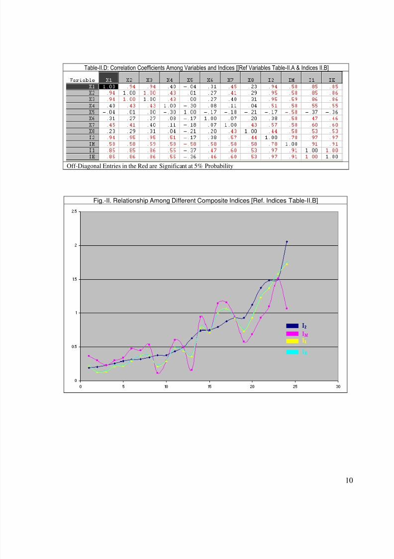
Secondly, I1 (as well as IE) has always alleviated the correlation between the index and
the constituent variables that were poorly dealt with by the PCA I2. For instance, the variables
x5 and x6 obtained correlation coefficients –0.17 and 0.38 with I2, which were alleviated to thevalues –0.37 and 0.47 by I1 (see Table-II.D). The trade off for this was a decline in the SSR
from 3.638772 (of I2) to 3.47997 (of I1), which is about 1.985 percent of the total variation inthe data. For the third set of data the decline in explanatory power was about 2.1 percent (of the
total) for alleviating the correlation (representation) of three variables, x4, x6, and x8 (see Table-
III.D). For the fourth set of data, correlation coefficients of five variables, x3, x4, x6, x7 and x8
were alleviated (see Table IV.D) for a trade-off of a decline in the explanatory power by 2.178
percent. From these observations it is clear that I1 alleviates representation of poorly correlated
variables for only a small trade-off of the overall explanatory power of the index.
Thirdly, a perusal of Fig.-II through Fig.-IV reveals that alleviation of representation of
weakly correlated variables by I1 alters the rank order of cases obtained by I2. While all indicesare ordered in accordance with I2 arranged in an ascending order (increasing monotonically),the non-monotonic movements of I1, IE and IM indicate to changes in the rank order suggested
by the PCA I2. Especially, the ranking of cases by the IM index is highly volatile.
Concluding Remarks: Construction of (composite) indices by the PCA is very common, butthis method has a preference for highly correlated variables to the poorly correlated variables
in the data set. Very often it fails to represent the poorly correlated variables. However, poor
correlation does not entail the marginal importance, since correlation coefficients among the
variables depend, apart from their linearity, also on their scatter, presence or absence of outliers, level of evolution of a system and intra-systemic integration among the different
constituents of the system. Under-evolved systems often throw up the data with poorly
correlated variables. If an index gives only marginal representation to the poorly correlatedvariables, it is elitist. The PCA index is often elitist, particularly for an under-evolved system.
In this paper we considered three alternative indices that determine weights given todifferent constituent variables on the principles different from the PCA. Two of the proposed
indices, the one that maximizes the sum of absolute correlation coefficient of the index with
the constituent variables and the other that maximizes the entropy-like function of thecorrelation coefficients between the index and the constituent variables are found to be very
close to each other. These indices alleviate the representation of poorly correlated variables for
some small reduction in the overall explanatory power (vis-à-vis the PCA index). These
indices are inclusive in nature, caring for the representation of the poorly correlated variables.
The third index obtained by maximization of the minimal correlation between the index andthe constituent variables cares most for the least correlated variable and in so doing becomes
egalitarian in nature.
It appears that neither the PCA index nor the egalitarian index can be fully justified. It
is more likely that the inclusive indices (I1 and IE) that strike a balance between individualrepresentation and overall representation (explanatory power) would perform better in real life.
Nevertheless, it is dependent on the analyst how to choose among the different indices.
8/14/2019 A Comparative Study of Various Inclusive Indices and the Index Constructed by the Principal Components Analysis
http://slidepdf.com/reader/full/a-comparative-study-of-various-inclusive-indices-and-the-index-constructed 6/14
6
References
• Adelman, I. And Morris, C.T. (1967) Society, Politics and Economic Development: A Quantitative
Approach, John Hopkins Press, Baltimore.
• Booysen, F. (2002) “An overview and evaluation of composite indices of development”, Social
Indicators Research, 59(2), pp.115-151.• Bradley, C. (1985) “The Absolute Correlation”, The Mathematical Gazette, 69 (447), pp. 12-17.
• Cahill, M.B. and Sánchez, N. (2001) “Using Principal Components to produce an Economic and Social
Development Index: An Application to Latin America and the U.S”, Atlantic Economic Journal, 29(3),
pp. 311-329.
• Jahan, S. (2005) “Measurement of Human Development: Evolution of the Human Development Index”
Draft Confidential Paper, http://hdr.undp.org/docs/training/oxford/readings/Jahan_HDI.pdf
• Kendall, MG and Stuart, A (1968): The Advanced Theory of Statistics, Charles Griffin & Co. London,
vol. 3. pp. 285-299.
• Michalos, A. C., Sharpe, A. and Muhajarine, N. (2006) “An Approach to a Canadian Index of Well
being”, http://creativecity.ca/cecc/downloads/indicators-2006/Michalos-Sharpe-Muhajarine-Approach-
CdnIndex-Wellbeing.pdf
• Michalos, A.C. (1980) North American Social Report, Vol. 1: Foundations, Population and Health, D.
Reidel, Dordrecht.
• Mishra, S.K. and Chopra, A. (1978) "Dimensions of Inter-district Disparities in Levels of Development
in MP". Indian Geographical Journal, 53. • Mishra, S.K. and Gaikwad, S.B. (1979) "Impact of Economic Development on Welfare and Living
Condition of People of MP". Indian Journal of Regional Science, 11(1). • Mishra, S.K. and Ngullie, M.L. (2003) "Locational Characteristics of Quality of Life in Dimapur Area,
Nagaland" in S Singh, et al. (eds) Environment, Locational Decisions and Regional Planning:
(Proceedings of International Conference). The Geographical Society of North Eastern Hill Region,
Shillong, 2003.
• Mishra, S. K. (2006-a) "Global Optimization by Differential Evolution and Particle Swarm Methods:
Evaluation on Some Benchmark Functions" SSRN: http://ssrn.com/abstract=933827
• Mishra, S. K. (2006-b) "Global Optimization by Particle Swarm Method: A Fortran Program". SSRN:
http://ssrn.com/abstract=921504
• Mishra, S. K. (2007) "Construction of an Index By Maximization of the Sum of its Absolute Correlation
Coefficients With the Constituent Variables" SSRN: http://ssrn.com/abstract=989088
• Munda G., Nardo M. (2005), "Constructing consistent composite indicators: the issue of weights," EUR
21834 EN , European Commission.
• Nardo M., Saisana M., Saltelli A., Tarantola S., Hoffman A., Giovannini E. (2005) Handbook on
constructing composite indicators: methodology and user guide. OECD Statistic Working Papers,
OECD, Paris. http://www.oecd.org/findDocument/0,2350,en_2649_201185_1_119684_1_1_1,00.html
• OECD (2003) Composite Indicators of Country Performance: A Critical Assessment , DST/IND(2003) 5,
Paris.
• Pal, M.N. (1975) “Regional Disparities in the Levels of Development in India,” Indian Journal of
Regional Science, 6(1).
• Saltelli, A. (2007) “Composite indicators between analysis and advocacy”, Social Indicators Research,
81(1), pp. 65-77.
• Salzman, J. (2003) “Methodological Choices Encountered in the Construction of Composite Indices of
Economic and Social Well-Being”, Center for the Study of Living Standards Ottawa, Ontario, Canada,
http://www.csls.ca/events/cea2003/salzman-typol-cea2003.pdf
8/14/2019 A Comparative Study of Various Inclusive Indices and the Index Constructed by the Principal Components Analysis
http://slidepdf.com/reader/full/a-comparative-study-of-various-inclusive-indices-and-the-index-constructed 7/14
7
Tables and Figures
Table-I.A: Indicator Variables for Construction of Composite Indices [Highly Correlated]
Sl. No. x1 x2 x3 x4 x5 x6 x7 x8
1 0.24746 0.62495 0.64798 0.29265 0.31671 0.45131 0.42735 0.08015
2 0.06005 0.04168 0.04671 0.08230 0.08601 0.06681 0.09165 0.093453 0.21551 0.22392 0.24862 0.43289 0.20651 0.19147 0.25072 0.25365
4 0.00467 0.00204 0.00207 0.00349 0.00036 0.00000 0.00060 0.000625 0.00492 0.00094 0.00148 0.00339 0.06350 0.04027 0.06567 0.06712
6 0.00000 0.00000 0.00000 0.00000 0.05235 0.02283 0.03290 0.033777 0.08357 0.05477 0.05515 0.09097 0.04490 0.02572 0.02829 0.029078 0.01201 0.00437 0.00596 0.01215 0.05122 0.02909 0.05154 0.05277
9 0.37148 0.48721 0.51445 0.86138 0.68763 0.92834 1.00000 1.0000010 0.13528 0.13168 0.14674 0.25535 0.21537 0.17546 0.19945 0.20215
11 0.03036 0.02167 0.02812 0.05547 0.03834 0.04408 0.07854 0.0801712 0.00517 0.00247 0.00273 0.00486 0.00093 0.00203 0.00179 0.00185
13 0.22977 0.23106 0.24024 0.39711 0.32794 0.40115 0.44139 0.4444614 0.10075 0.13038 0.13673 0.22851 0.09439 0.09460 0.09475 0.09659
15 0.24962 0.29629 0.32783 0.57561 0.25105 0.24130 0.28731 0.2903416 1.00000 1.00000 1.00000 0.99986 1.00000 1.00000 0.97507 0.3112717 0.09500 0.09544 0.11392 0.21605 0.07342 0.14685 0.21159 0.21435
18 0.00692 0.00531 0.00670 0.01292 0.04406 0.01908 0.03115 0.0319919 0.15371 0.23098 0.24742 0.41749 0.12368 0.12069 0.12515 0.12731
20 0.12861 0.14135 0.16284 0.29275 0.12030 0.15318 0.18549 0.1881121 0.48198 0.64806 0.63219 0.99368 0.45382 0.62726 0.56703 0.5697822 0.38457 0.58160 0.60495 1.00000 0.33558 0.38847 0.40284 0.40595
23 0.26555 0.46573 0.46191 0.73598 0.18568 0.29337 0.30829 0.3113624 0.00167 0.00766 0.01020 0.02037 0.00000 0.00067 0.00000 0.00000
Table-I.B: Composite Indices Obtained by Different Methods [Ref Variables Table-I.A]
Sl I2 IM I1 IE Sl I2 IM I1 IE1 1.079414 0.36413 1.056081 1.057227 13 0.937040 0.538982 0.943005 0.942854
2 0.198332 0.118026 0.199657 0.199622 14 0.330894 0.166297 0.330367 0.330430
3 0.689426 0.378483 0.691368 0.691366 15 0.853914 0.445329 0.855006 0.855063
4 0.004868 0.003617 0.004838 0.004840 16 2.564157 1.062231 2.519834 2.522082
5 0.088566 0.05599 0.090258 0.090194 17 0.394920 0.246977 0.400026 0.399850
6 0.051678 0.026676 0.052226 0.052208 18 0.056314 0.030495 0.056834 0.056818
7 0.143639 0.083649 0.142771 0.142825 19 0.517690 0.246265 0.516119 0.516253
8 0.078064 0.049483 0.079316 0.079270 20 0.465196 0.256904 0.467424 0.467383
9 2.009407 1.123417 2.024317 2.023906 21 1.694556 0.886993 1.694174 1.694394
10 0.504692 0.269166 0.506018 0.506020 22 1.380812 0.686166 1.379353 1.379588
11 0.129412 0.085831 0.131575 0.131496 23 1.014063 0.515119 1.014063 1.014188
12 0.007571 0.00498 0.007550 0.007552 24 0.012471 0.002931 0.012337 0.012345
Table-I.C: Correlation of Variables with Different Composite [Ref Variables Table-I.A & Indices I.B]Var x1 x2 x3 x4 x5 x6 x7 x8 SAR SSR
I2 0.946761 0.952049 0.953948 0.929121 0.966369 0.979891 0.970493 0.788174 7.486806 7.033167
IM 0.888074 0.888074 0.891592 0.942540 0.931946 0.966049 0.968422 0.888074 7.364771 6.788959
I1 0.943117 0.948906 0.950980 0.931407 0.964780 0.980130 0.971582 0.796657 7.487560 7.031865
IE 0.943282 0.949048 0.951116 0.931311 0.964854 0.980123 0.971538 0.796286 7.487558 7.031977
SAS=Sum of Absolute Correlation Coefficients; SSR=Sum of Squared Correlation Coefficients

8/14/2019 A Comparative Study of Various Inclusive Indices and the Index Constructed by the Principal Components Analysis
http://slidepdf.com/reader/full/a-comparative-study-of-various-inclusive-indices-and-the-index-constructed 8/14
8
Table-I.D: Correlation Coefficients Among Variables and Indices [[Ref Variables Table-I.A & Indices I.B]
Off-Diagonal Entries in the Red are Significant at 5% Probability
Fig.-I. Relationship Among Different Composite Indices [Ref. Indices Table-I.B]
8/14/2019 A Comparative Study of Various Inclusive Indices and the Index Constructed by the Principal Components Analysis
http://slidepdf.com/reader/full/a-comparative-study-of-various-inclusive-indices-and-the-index-constructed 9/14
9
Table-II.A: Indicator Variables for Construction of Composite Indices [Poorly Correlated]
Sl. No. x1 x2 x3 x4 x5 x6 x7 x8
1 0.24746 0.62495 0.64798 0.98526 0.53466 0.39441 0.20494 0.380592 0.06005 0.04168 0.04671 0.81953 0.34072 0.30900 0.24717 0.42699
3 0.21551 0.22392 0.24862 0.75169 0.07558 1.00000 0.05978 0.74561
4 0.00467 0.00204 0.00207 0.62952 0.69993 0.62658 0.08976 0.000005 0.00492 0.00094 0.00148 0.37364 0.40331 0.46080 0.73544 0.14438
6 0.00000 0.00000 0.00000 0.00382 0.44343 0.80199 0.00000 0.374797 0.08357 0.05477 0.05515 0.14273 0.81714 0.51229 0.66290 0.80686
8 0.01201 0.00437 0.00596 0.00000 0.78624 0.70126 0.58950 0.337159 0.37148 0.48721 0.51445 0.94753 0.32142 0.83483 1.00000 1.00000
10 0.13528 0.13168 0.14674 0.75008 0.53330 0.89228 0.75648 0.2937011 0.03036 0.02167 0.02812 0.52677 0.50320 0.27864 0.16180 0.2858312 0.00517 0.00247 0.00273 0.81192 0.67010 0.13235 0.18545 0.20847
13 0.22977 0.23106 0.24024 1.00000 0.50611 0.43962 0.72437 0.6129314 0.10075 0.13038 0.13673 0.07053 0.60184 0.00000 0.62472 0.34690
15 0.24962 0.29629 0.32783 0.20606 1.00000 0.48399 0.14823 0.50274
16 1.00000 1.00000 1.00000 0.84209 0.50033 0.79510 0.79321 0.1950717 0.09500 0.09544 0.11392 0.35220 0.52443 0.29656 0.35003 0.2532218 0.00692 0.00531 0.00670 0.79915 0.57212 0.51521 0.25717 0.1121919 0.15371 0.23098 0.24742 0.21522 0.60198 0.81727 0.56037 0.64080
20 0.12861 0.14135 0.16284 0.45753 0.00000 0.80053 0.72405 0.6181421 0.48198 0.64806 0.63219 0.74621 0.40213 0.62240 0.95548 0.50585
22 0.38457 0.58160 0.60495 0.63480 0.60728 0.31909 0.90734 0.9564123 0.26555 0.46573 0.46191 0.35542 0.84484 0.91816 0.29377 0.41605
24 0.00167 0.00766 0.01020 0.14215 0.25842 0.18922 0.61566 0.49687
Table-II.B: Composite Indices Obtained by Different Methods [Ref Variables Table-II.A]
Sl I2 IM I1 IE Sl I2 IM I1 IE1 1.125449 0.691817 0.940740 0.956974 13 0.928561 0.945244 0.929377 0.936279
2 0.437819 0.605365 0.486051 0.487176 14 0.377971 0.117180 0.223698 0.2352153 0.881326 1.161851 1.066787 1.062896 15 0.633218 0.160483 0.363657 0.382202
4 0.210942 0.300350 0.139033 0.144432 16 2.060263 1.067789 1.727033 1.755478
5 0.348284 0.531365 0.376710 0.378368 17 0.380738 0.293795 0.297690 0.305053
6 0.195389 0.364572 0.229844 0.229819 18 0.311787 0.475802 0.296464 0.299828
7 0.499766 0.496664 0.448307 0.456081 19 0.747547 0.725261 0.725769 0.732526
8 0.291834 0.341532 0.227550 0.233963 20 0.793596 1.142705 1.004999 0.999831
9 1.505166 1.513450 1.589971 1.596008 21 1.485616 1.098683 1.376886 1.39183
10 0.745028 0.946549 0.788813 0.791959 22 1.375272 0.931124 1.233855 1.250889
11 0.263581 0.300388 0.223115 0.227638 23 0.933953 0.580389 0.741194 0.757039
12 0.232466 0.236987 0.139987 0.147184 24 0.319021 0.447995 0.372676 0.373255
Table-II.C: Correlation of Variables with Different Composite [Ref Variables Table-II.A & Indices II.B] Var x1 x2 x3 x4 x5 x6 x7 x8 SAR SSR
I2 0.936702 0.951937 0.953816 0.511988 -0.166793 0.379617 0.566275 0.436675 4.903802 3.638772
IM 0.584170 0.577289 0.585303 0.577289 -0.577289 0.577289 0.577289 0.577289 4.633205 2.683408
I1 0.847254 0.852676 0.857515 0.547537 -0.372181 0.465816 0.600943 0.532267 5.076190 3.479970
IE 0.853871 0.859913 0.864598 0.546234 -0.360623 0.461316 0.600651 0.528412 5.075618 3.497309
SAS=Sum of Absolute Correlation Coefficients; SSR=Sum of Squared Correlation Coefficients
8/14/2019 A Comparative Study of Various Inclusive Indices and the Index Constructed by the Principal Components Analysis
http://slidepdf.com/reader/full/a-comparative-study-of-various-inclusive-indices-and-the-index-constructed 10/14
10
Table-II.D: Correlation Coefficients Among Variables and Indices [[Ref Variables Table-II.A & Indices II.B]
Off-Diagonal Entries in the Red are Significant at 5% Probability
Fig.-II. Relationship Among Different Composite Indices [Ref. Indices Table-II.B]
8/14/2019 A Comparative Study of Various Inclusive Indices and the Index Constructed by the Principal Components Analysis
http://slidepdf.com/reader/full/a-comparative-study-of-various-inclusive-indices-and-the-index-constructed 11/14
11
Table-III.A: Indicator Variables for Construction of Composite Indices [Poorly Correlated]
Sl. No. x1 x2 x3 x4 x5 x6 x7 x8
1 0.24746 0.62495 0.64530 1.00000 0.48439 0.25953 0.10990 0.433272 0.06005 0.04168 0.36793 0.90801 0.37204 0.33344 0.29963 0.48453
3 0.21551 0.22392 0.12246 0.67552 0.04525 1.00000 0.00000 0.80680
4 0.00467 0.00204 0.38290 0.73010 0.78395 0.69234 0.13950 0.000005 0.00492 0.00094 0.07724 0.44322 0.44683 0.50271 0.92201 0.14866
6 0.00000 0.00000 0.09666 0.03003 0.49347 0.86528 0.01387 0.446197 0.08357 0.05477 0.74887 0.14521 0.88956 0.56247 0.84635 0.97911
8 0.01201 0.00437 0.00000 0.02033 0.85454 0.75777 0.74490 0.391729 0.37148 0.48721 0.89033 0.70394 0.11269 0.51601 0.87274 0.79682
10 0.13528 0.13168 0.32328 0.75292 0.52323 0.89464 0.89386 0.2737811 0.03036 0.02167 0.75736 0.59169 0.56191 0.31146 0.19800 0.3168412 0.00517 0.00247 0.39756 0.93403 0.75234 0.17698 0.25891 0.25563
13 0.22977 0.23106 0.92212 0.96992 0.44989 0.32784 0.75502 0.5613014 0.10075 0.13038 0.44711 0.00289 0.64341 0.00000 0.77143 0.38477
15 0.24962 0.29629 0.97997 0.00000 1.00000 0.44172 0.09592 0.49252
16 1.00000 1.00000 0.51977 0.52392 0.17676 0.44431 0.62379 0.1054417 0.09500 0.09544 0.38364 0.32430 0.57030 0.28660 0.37963 0.2187718 0.00692 0.00531 0.51589 0.91611 0.63214 0.56833 0.33681 0.1243019 0.15371 0.23098 0.63596 0.08082 0.63192 0.83975 0.67841 0.73261
20 0.12861 0.14135 1.00000 0.40818 0.00000 0.80856 0.85891 0.6784921 0.48198 0.64806 0.23095 0.41917 0.29050 0.42237 0.99341 0.37558
22 0.38457 0.58160 0.82704 0.29142 0.55329 0.20774 1.00000 1.0000023 0.26555 0.46573 0.68763 0.09593 0.86276 0.87165 0.26973 0.37692
24 0.00167 0.00766 0.05871 0.17606 0.31965 0.23676 0.79869 0.61079
Table-III.B: Composite Indices Obtained by Different Methods [Ref Variables Table-III.A]
Sl I2 IM I1 IE Sl I2 IM I1 IE1 0.651733 0.818771 0.748653 0.743082 13 0.657447 1.036658 0.896935 0.884985
2 0.213099 0.728379 0.424731 0.409833 14 0.285439 0.478063 0.362768 0.3597843 0.385989 0.514145 0.325942 0.328320 15 0.337320 0.272618 0.213000 0.221695
4 -0.155489 0.136302 -0.166052 -0.170653 16 1.409851 0.770389 1.118269 1.142971
5 0.069696 0.349755 0.126488 0.121414 17 0.141003 0.325231 0.168031 0.165503
6 -0.121018 -0.076426 -0.288529 -0.281552 18 0.018980 0.420868 0.134952 0.124445
7 0.324372 0.697248 0.409374 0.405274 19 0.401334 0.400253 0.305872 0.313528
8 -0.104151 0.107688 -0.218741 -0.215419 20 0.675407 0.638039 0.747407 0.749557
9 1.032543 1.064830 1.143588 1.143399 21 0.896517 0.736519 0.808321 0.817525
10 0.261768 0.488108 0.266733 0.264948 22 1.016361 1.109601 1.107143 1.107846
11 0.151442 0.460668 0.285860 0.277170 23 0.380115 0.123095 0.117860 0.134196
12 0.001039 0.624263 0.224154 0.206151 24 0.196108 0.553662 0.322833 0.315328
Table-III.C: Correlation of Variables with Different Composite [Ref Variables Table-III.A & Indices III.B] Var x1 x2 x3 x4 x5 x6 x7 x8 SAR SSR
I2 0.892224 0.894489 0.481349 0.103277 -0.523490 -0.169397 0.423706 0.354061 3.841993 2.446160
IM 0.468925 0.49504 0.468925 0.468925 -0.468930 -0.468930 0.468925 0.468925 3.7775160 1.7843010
I1 0.719992 0.736127 0.542095 0.296654 -0.557102 -0.360363 0.474812 0.412594 4.099740 2.278047
IE 0.733698 0.748858 0.541317 0.282511 -0.557073 -0.348860 0.474634 0.411634 4.098585 2.298691
SAS=Sum of Absolute Correlation Coefficients; SSR=Sum of Squared Correlation Coefficients

8/14/2019 A Comparative Study of Various Inclusive Indices and the Index Constructed by the Principal Components Analysis
http://slidepdf.com/reader/full/a-comparative-study-of-various-inclusive-indices-and-the-index-constructed 12/14
12
Table-III.D: Correlation Coefficients Among Variables and Indices [[Ref Variables Table-III.A & Indices III.B]
Off-Diagonal Entries in the Red are Significant at 5% Probability
Fig.-III. Relationship Among Different Composite Indices [Ref. Indices Table-III.B]
8/14/2019 A Comparative Study of Various Inclusive Indices and the Index Constructed by the Principal Components Analysis
http://slidepdf.com/reader/full/a-comparative-study-of-various-inclusive-indices-and-the-index-constructed 13/14
13
Table-IV.A: Indicator Variables for Construction of Composite Indices [Poorly Correlated]
Sl. No. x1 x2 x3 x4 x5 x6 x7 x8
1 0.24746 0.62495 0.59656 1.00000 0.47371 0.23122 0.09670 0.436592 0.06005 0.04168 0.36946 0.92859 0.37870 0.33857 0.31651 0.48790
3 0.21551 0.22392 0.10233 0.67130 0.03881 1.00000 0.00000 0.80370
4 0.00467 0.00204 0.38867 0.76192 0.80181 0.70615 0.16189 0.000005 0.00492 0.00094 0.07874 0.48210 0.45608 0.51151 0.94886 0.14633
6 0.00000 0.00000 0.09857 0.07938 0.50411 0.87856 0.03202 0.453927 0.08357 0.05477 0.75502 0.18382 0.90495 0.57300 0.87533 1.00000
8 0.01201 0.00437 0.00000 0.06887 0.86906 0.76964 0.77069 0.396479 0.37148 0.48721 0.85708 0.66173 0.06831 0.44908 0.82186 0.72743
10 0.13528 0.13168 0.31517 0.76225 0.52109 0.89514 0.90931 0.2624911 0.03036 0.02167 0.76607 0.62239 0.57439 0.31835 0.21469 0.3173712 0.00517 0.00247 0.40348 0.96070 0.76983 0.18635 0.28270 0.26163
13 0.22977 0.23106 0.91405 0.96157 0.43794 0.30438 0.74877 0.5354414 0.10075 0.13038 0.44165 0.03303 0.65224 0.00000 0.79399 0.38547
15 0.24962 0.29629 0.96482 0.00000 1.00000 0.43284 0.09410 0.47866
16 1.00000 1.00000 0.43752 0.47409 0.10797 0.37067 0.57185 0.0804717 0.09500 0.09544 0.37933 0.34760 0.58006 0.28451 0.38762 0.2050818 0.00692 0.00531 0.52312 0.94252 0.64490 0.57948 0.35916 0.1244919 0.15371 0.23098 0.62319 0.09259 0.63828 0.84447 0.69729 0.73891
20 0.12861 0.14135 1.00000 0.42275 0.00000 0.81025 0.87508 0.6781221 0.48198 0.64806 0.17777 0.37246 0.26676 0.38038 0.97977 0.33419
22 0.38457 0.58160 0.78475 0.24730 0.54181 0.18436 1.00000 0.9880323 0.26555 0.46573 0.65625 0.07961 0.86657 0.86189 0.26836 0.35843
24 0.00167 0.00766 0.05916 0.22005 0.33267 0.24674 0.82941 0.62545
Table-IV.B: Composite Indices Obtained by Different Methods [Ref Variables Table-IV.A]
Sl I2 IM I1 IE Sl I2 IM I1 IE1 0.531098 0.925353 0.182593 0.221711 13 0.494170 1.150057 0.356003 0.389267
2 0.094656 0.841262 -0.091308 -0.063412 14 0.213905 0.552373 0.368402 0.3762313 0.244917 0.652166 -0.058258 -0.022551 15 0.219757 0.380701 0.229124 0.246618
4 -0.269473 0.306820 -0.582179 -0.552165 16 1.335452 0.876993 0.845077 0.892770
5 -0.027031 0.490731 -0.127556 -0.105971 17 0.056142 0.418350 -0.019365 -0.002165
6 -0.213773 0.074337 -0.307416 -0.290635 18 -0.110342 0.580703 -0.384740 -0.353482
7 0.159879 0.865343 0.346443 0.364903 19 0.247875 0.563812 0.275847 0.298739
8 -0.208298 0.278327 -0.226687 -0.207978 20 0.498274 0.793722 0.525584 0.549162
9 0.861887 1.136477 0.753595 0.787038 21 0.794450 0.813497 0.580709 0.614520
10 0.109549 0.674369 -0.154601 -0.117721 22 0.866519 1.180156 0.965953 0.991286
11 0.036302 0.576362 -0.048515 -0.028578 23 0.245266 0.269341 0.075130 0.103762
12 -0.104548 0.741485 -0.305911 -0.279128 24 0.111973 0.650391 0.223784 0.235157
Table-IV.C: Correlation of Variables with Different Composite [Ref Variables Table-IV.A & Indices IV.B] Var x1 x2 x3 x4 x5 x6 x7 x8 SAR SSR
I2 0.909969 0.907878 0.379255 0.007804 -0.566301 -0.280218 0.359750 0.266566 3.677741 2.395877
IM 0.448620 0.469218 0.448620 0.448620 -0.484044 -0.448620 0.448620 0.448620 3.644981 1.662023
I1 0.725619 0.732870 0.466649 -0.265822 -0.432589 -0.350864 0.542376 0.514956 4.031744 2.221633
IE 0.737322 0.744495 0.466621 -0.250255 -0.440816 -0.345379 0.537675 0.508116 4.030679 2.239160
SAS=Sum of Absolute Correlation Coefficients; SSR=Sum of Squared Correlation Coefficients
8/14/2019 A Comparative Study of Various Inclusive Indices and the Index Constructed by the Principal Components Analysis
http://slidepdf.com/reader/full/a-comparative-study-of-various-inclusive-indices-and-the-index-constructed 14/14
14
Table-IV.D: Correlation Coefficients Among Variables and Indices [[Ref Variables Table-IV.A & Indices IV.B]
Off-Diagonal Entries in the Red are Significant at 5% Probability
Fig.-IV. Relationship Among Different Composite Indices [Ref. Indices Table-IV.B]
Note: FORTRAN codes for computing inclusive and egalitarian indices may be obtained on
request to [email protected]