a comparative study of three image matcing algorithms...
TRANSCRIPT

Utah State UniversityDigitalCommons@USU
All Graduate Theses and Dissertations Graduate Studies, School of
1-1-2011
A Comparative Study of Three Image MatcingAlgorithms: Sift, Surf, and FastMaridalia GuerreroUtah State University
This Thesis is brought to you for free and open access by the GraduateStudies, School of at DigitalCommons@USU. It has been accepted forinclusion in All Graduate Theses and Dissertations by an authorizedadministrator of DigitalCommons@USU. For more information, pleasecontact [email protected].
Recommended CitationGuerrero, Maridalia, "A Comparative Study of Three Image Matcing Algorithms: Sift, Surf, and Fast" (2011). All Graduate Theses andDissertations. Paper 1040.http://digitalcommons.usu.edu/etd/1040

A COMPARATIVE STUDY OF THREE IMAGE MATCHING ALGORITHMS: SIFT, SURF,
AND FAST
by
Maridalia Guerrero Peña
A thesis submitted in partial fulfillment
of the requirements for the degree
of
MASTER OF SCIENCE
in
Civil and Environmental Engineering
Approved:
______________________________ ________________________________
Dr. Robert T.Pack Dr. James A. Bay
Major Professor Committee Member
_________________________________ ________________________________
Dr. Xiaojun Qi
Committee Member
UTAH STATE UNIVERSITY
Logan, Utah
2011
Dr. Mark R. McLellan Vice
President for Research and Dean of
the School of Graduate Studies

ii
Copyright © Maridalia Guerrero, 2011
All Rights Reserved

iii
ABSTRACT
A Comparative Study Of Three Image Matching Algorithms: Sift, Surf, And Fast
by
Maridalia Guerrero Peña, Master of Science
Utah State University, 2011
Major Professor: Dr. Robert Pack
Department: Civil and Environmental Engineering
A new method for assessing the performance of popular image matching algorithms
is presented. Specifically, the method assesses the type of images under which each of the
algorithms reviewed herein perform to its maximum or highest efficiency. The efficiency
is measured in terms of the number of matches founds by the algorithm and the number
of type I and type II errors encountered when the algorithm is tested against a specific
pair of images. Current comparative studies asses the performance of the algorithms
based on the results obtained in different criteria such as speed, sensitivity, occlusion, and
others. These studies are an important resource to understand the behavior of the
algorithms and their influence on the results obtained. But they do not account for the
inherent characteristics of the algorithms that derive the process through which the
matching features are evaluated, filtered, and finally selected. Moreover, these methods
cannot be used to predict the efficiency or level of accuracy that could be reached by
using one algorithm or the other depending on of the type of images. This ability to
predict performance becomes handy in situations where time is a limiting factor in a

iv
project because it allows one to quickly predict which algorithm will save the most time
and resources.
This study addresses the limitations of the existing comparative tools and delivers a
generalized criterion to determine beforehand the level of efficiency expected from a
matching algorithm given the type of images evaluated. The algorithms and the
respective images used within this work are divided into two groups: Feature-Based and
Texture-Based. And from this broad classification only three of the most widely used
algorithms are assessed: SIFT, SURF, and FAST. The latter is the only one belonging to
the feature-based category. Three types of images were evaluated in this study: planar
surfaces, cluttered background, and repetitive patterns. For the purpose of matching
planar and very “edgy” objects, such as a boat or a building, the feature-based algorithm
(FAST) was found to perform with fewer detection errors than the texture-based
algorithms. Conversely, when the images evaluated corresponded to cluttered
backgrounds or considerably busy scenes, the texture-based detected a larger number of
features and matches. The results of each algorithm are evaluated and presented. The
number of false matches is manually determined and also presented in the final results.
The conclusion and recommendations for feature works in this subject lead towards the
improvement of these powerful algorithms to achieve a higher level of efficiency within
the scope of its performance.
(120 pages)

v
DEDICATION
I dedicate this thesis to my parents, Ydalia and Ezequiel, for their unconditional
love and support. Because despite distance you were always willing to pick up the phone
and make me feel home again, I deeply love you both. To my older sister, Olga, for her
genuine interest in my work and her continued motivation, I love you so much. To my
oldest brother, Carlos, for those long emails full of advice, I thank you and love you. I
also would like to thank my remaining sisters, Paola, Cristy, and Yuleisis for being part
of my life and giving me so much love.
I couldn‟t have done any of this without your unconditional love and support.

vi
ACKNOWLEDGMENTS
I would like to express my deepest gratitude to my advisor and major professor, Dr.
Robert Pack, for introducing me to the wonderful world of photogrammetry and
computer vision. His guidance, support, and patient through this journey were endless. I
wish to thank my committee members, Dr. James Bay and Dr. Xiaojun Qi, for their
advice and continuous support. I also thank Keith Blonquist for his selfless help and for
sharing his wide knowledge on this subject with me. I would also like to thank Erick
Conde for his willingness to listen to my doubts and concerns and his thoughtful
suggestions.
The financial support of our sponsor, Mr. Dean Cook, from the Naval Air Warfare
Center, Weapons Division is gratefully acknowledged.
Last but not least, I would like to thank family and friends for believing in me and
cheering me up when I needed it the most. I love you all.
Eng. Maridalia Guerrero Peña
vii
CONTENTS
Page
ABSTRACT ....................................................................................................................... iii
DEDICATION .................................................................................................................... v
ACKNOWLEDGMENTS ................................................................................................. vi
LIST OF TABLES ............................................................................................................. ix
LIST OF FIGURES ............................................................................................................ x
LIST OF EQUATIONS ................................................................................................... xiv
CHAPTER
1. INTRODUCTION .......................................................................................................... 1
1.1 Problem Statement ............................................................................................... 1 1.2 Scope and Purpose ............................................................................................... 3
1.3 Organization ......................................................................................................... 4
2. LITERATURE REVIEW ............................................................................................... 5
2.1 Literature Overview: Introduction to corners, edges and texture based detectors 5 2.2 Feature-based matching algorithms: corner and edge detectors .......................... 6 2.3 FAST Corner Detector ......................................................................................... 7
2.4 Textured-Based Algorithms ............................................................................... 11 2.5 Lowe‟s Approach ............................................................................................... 12
2.6 Mikolajczyk and Schmid‟s Approach ................................................................ 14 2.7 SIFT, PCA-SIFT and SURF texture-based matching algorithms ...................... 14
2.8 Scale Invariant Feature Transform: SIFT........................................................... 15 2.9 Principal Component Analysis for SIFT: PCA-SIFT ........................................ 16 2.10 Speeded-Up Robust Feature: SURF .................................................................. 17 2.11 Commercial Implementations ............................................................................ 17
2.12 Previous Work On Matching Algorithms Comparison ..................................... 19
3. METHODOLOGY ....................................................................................................... 22
3.1 Overview ............................................................................................................ 22 3.2 Source Of Data: Images and Algorithms ........................................................... 22 3.3 Experimental Process ......................................................................................... 26
3.3.1 Data selection .............................................................................................. 27

viii
3.3.2 Image pairs .................................................................................................. 27
3.3.3 Feature detection ......................................................................................... 27 3.3.4 Manual detection of matches candidates .................................................... 30 3.3.5 Automated detection of matching ............................................................... 30
3.3.6 Evaluating the results .................................................................................. 31 3.3.7 Final comparison ......................................................................................... 31
4. DATA ANALYSIS ....................................................................................................... 32
4.1 Feature Detection ............................................................................................... 32
4.1.1 SIFT feature detection................................................................................. 32 4.1.2 SURF feature detection ............................................................................... 34
4.1.3 FAST feature detection ............................................................................... 36
4.2 Feature Matching................................................................................................ 37
4.2.1 SIFT feature matching ................................................................................ 37 4.2.2 SURF feature matching............................................................................... 37 4.2.3 FAST feature matching ............................................................................... 39
5. RESULTS AND CONCLUSIONS............................................................................... 40
5.1 General Overview .............................................................................................. 40 5.2 Feature Detection Results................................................................................... 40
5.3 Feature Matching Results ................................................................................... 47
5.4 Conclusions ........................................................................................................ 52
6. RECOMMENDATIONS .............................................................................................. 54
REFERENCES ................................................................................................................. 56
APPENDICES .................................................................................................................. 58
Appendix A. Feature Detection Images ........................................................................ 59 Appendix B. Matches.................................................................................................... 72 Appendix C. Matches found after threshold modification ............................................ 81
Appendix D. Type II error detection (Mismatches) ...................................................... 85 Appendix E. Manual matching for detected features .................................................... 94

ix
LIST OF TABLES
Table Page
1 Results presented by Lowe showing the efficiency of SIFT ................................... 13
2 A comparison of keypoint matching and computed transform a
ccuracy between the SIFT library and David Lowe's SIFT executable ................... 38
3 Number of feature detected in the image dataset for the three
algorithms ................................................................................................................ 42
4 Matching performance for SIFT .............................................................................. 49
5 Matching performance for SURF ............................................................................ 49
6 Matching performance for FAST............................................................................. 50
7 Type I and Type II errors detection for SIFT matches ............................................ 52
8 Type I and Type II errors detection for SURF matches........................................... 52

x
LIST OF FIGURES
Figure Page
1 (a) Wallis filtered image; (b) Enlarged area showing FAST interest
operator results on Wallis filtered image; (c) Enlarged area
showing FAST operator results on original iamge. .............................................. 10
2 Model of planar objects are in top row. ................................................................ 13
3 Images used for the SIFT, PCA-SIFT and SURF comparative
study. ..................................................................................................................... 21
4 The four different datasets used as the input images for the tests.
(a) Repetitive pattern and clutter; (b) Edges and corners (Brick
Wall); (c) The Haddock Boat (Planar Surfaces); (d) Rotation. ............................ 24
5 Results presented by Rob Hess with the implementation of the
SIFT algorithm for object recognition. Top: SIFT features detected
in two images. Bottom: SIFT featured matches between the two
images. .................................................................................................................. 25
6 FAST corner detection demonstration. ................................................................. 26
7 Windows (First Pair). ............................................................................................ 28
8 The Boat (Third Pair). ........................................................................................... 29
9 Brick Wall (Second Pair). ..................................................................................... 28
10 The building (Fourth Pair). ................................................................................... 29
11 SIFT feature detection algorithm (Taken from Jason Clemens). .......................... 32
12 If the contrast between two interest points is different (dark on
light background vs. light on dark background), the candidate is
not considered a valuable match (Bay 2008). ....................................................... 38
13 Features detected in the Window image pair (Images A and B). ......................... 43
14 Features detected in the Brick Wall Image pair (Images A and B). ..................... 43
15 Features detected in the Boat Image pair (Images A and B). ............................... 44
16 Features detected in the Building Image pair (Images A and B). ......................... 44

xi
17 Overall view of the features detected on each image. .......................................... 46
18 SIFT Features detected – Window Image Pair. .................................................... 60
19 SIFT Features detected – Brick Wall Image Pair. ................................................ 61
20 SIFT features detected – Boat Image Pair. ........................................................... 62
21 SIFT Features detected – Building Image Pair. .................................................... 63
22 SURF Features detected – Window Image Pair. .................................................. 64
23 SURF Features detected – Brick Wall Image Pair................................................ 65
24 SURF Features – Boat Image Pair. ....................................................................... 66
25 SURF Features detected – Building Image Pair. .................................................. 67
26 FAST Features detected – Window Image Pair. ................................................... 68
27 FAST Features detected – Brick Wall Image Pair. ............................................... 69
28 FAST Features detected – Boat Image Pair. ......................................................... 70
29 FAST Features detected – Building Image Pair. .................................................. 71
30 SIFT Matches – Window Image Pair.................................................................... 73
31 SIFT Matches – Brick Image Pair. ....................................................................... 74
32 SIFT Matches – Boat Image Pair. ......................................................................... 75
33 SIFT Matches – Building Image Pair. .................................................................. 76
34 SURF Matches – Window Image Pair. ................................................................. 77
35 SURF Matches – Brick Wall Image Pair. ............................................................. 78
36 SURF Features for third pair – Boat Image Pair. .................................................. 79
37 SURF Matches – Building Image Pair.................................................................. 80
38 SIFT Matches after reducing the threshold ratio from 0.49 to 0.35.
Brick Wall Image Pair. ......................................................................................... 82

xii
39 SIFT Matches after reducing the threshold ratio from 0.49 to 0.35.
Brick Wall and Building Image Pairs. .................................................................. 83
40 SURF Matches after varying the threshold value – Brick Wall and
Building Image Pairs............................................................................................. 84
41 SIFT incorrect matches – Window Image Pair. .................................................... 86
42 SIFT Incorrect Matches – Brick Wall Image Pair. ............................................... 87
43 SIFT incorrect matches – Boat Image Pair. .......................................................... 88
44 SIFT incorrect matches - Building Image Pair. .................................................... 89
45 SURF incorrect matches – Window Image Pair. .................................................. 90
46 SURF incorrect matches – Brick Wall Image Pair. .............................................. 91
47 SURF incorrect matches – Boat Image Pair. ........................................................ 92
48 SURF incorrect matches – Building Image Pair. .................................................. 93
49 Manually detected potential matches for SIFT – Window Image
Pair. ....................................................................................................................... 95
50 Manually detected potential matches for SIFT –Brick Wall Image
Pair. ....................................................................................................................... 95
51 Manually detected potential matches for SIFT –Boat Image pair. ....................... 95
52 Manually detected potential matches for SIFT-Building Image
Pair. ....................................................................................................................... 95
53 Manually detected potential matches for SURF-Window Image
Pair. ....................................................................................................................... 95
54 Manually detected potential matches for SURF – Brick Wall
Image Pair. ............................................................................................................ 95
55 Manually detected potential matches for SURF – Boat Image Pair. .................... 95
56 Manually detected potential matches for SURF-Building Image
Pair. ....................................................................................................................... 95
57 Manually detected potential matches for FAST-Window Image
Pair. ....................................................................................................................... 95

xiii
58 Manually detected potential matches for FAST –Brick Wall Image
Pair. ....................................................................................................................... 95
59 Manually detected potential matches for FAST-Boat Image Pair. ....................... 95
60 Manually detected potential matches for FAST-Building Image
Pair. ....................................................................................................................... 95

xiv
LIST OF EQUATIONS
Equation Page
1 Line code to calculate width and height for SURF feature
points ..................................................................................................................... 34
2 Function to draw SURF feature points. ................................................................ 35
3 Two variable Hessian matrix used in the detection of
feature points with OpenSurf. ............................................................................... 35
4 Equation used to calculate the determinant for the Hessian
matrix. ................................................................................................................... 35
5 Equation used to determine the effectiveness of the
number of features detected for a given image pair. ............................................. 48

CHAPTER 1
INTRODUCTION
1.1 Problem Statement
Feature detection and image matching represent two important tasks in
photogrammetry. Their application continues to grow in a variety of fields day by day.
From simple photogrammetry tasks such as feature recognition, to the development of
sophisticated 3D modeling software, there are several applications where image matching
algorithms play an important role. Moreover, this has been a very active area of research
in the recent decades and as indicated by the tremendous amount of work and
documentation published around this. As needs change and become more demanding,
researches are encouraged to develop new technologies in order to fulfill these needs.
In this tenor, is worth mentioning that many methods published with source code
satisfy the everyday needs of photogrammetry and computer vision including feature
detection, matching and 3D modeling. This latter task has been an ongoing research topic
in computer vision and photogrammetry for many years now. Obtaining 3D models is
considered in many cases the ultimate purpose of feature detection and subsequent
matching. More than a decade ago, the applications associated with 3D models and object
reconstruction were mainly for the purpose of visual inspection and robotics. Today,
these applications now include the use of 3D models in computer graphics, virtual reality,
communication and others.
But achieving highly reliable matching results from a pair of images is the task that
some of the most popular matching methods are trying to accomplish. But none have

2
been universally accepted. And it seems that the selection the adequate method to
complete a matching task significantly depends on the type of image to be matched and
in the variations within an image and its matching pair in one or many of the following
parameters:
a) Scale: At least two elements of the set of images views have different scales
b) Occlusion: Is the concept that two objects that are spatially separated in the 3D
world might interfere with each other in the projected 2D image plane. For single-
view tasks, such as object recognition, occlusions are typically considered a
nuisance requiring more robust algorithms (Hoiem et al., 2007)
c) Orientation: The images views are rotated with respect to each other . A maximum
orientation of 30 ̊ is a typical maximum value for most of the algorithms to
perform a reliable match
d) Object to be matched: Whether is a planar, textured or edgy object
e) Clutter: This refers to the conditions of the image background. It is often difficult
form the algorithm to understand the boundaries of the object of interest when it
has a cluttered background
f) Illumination: Changes in illumination also represent a typical problem for
accurate feature matching
Current image matching algorithms may perform acceptably well in presence of
some of the image conditions described above. But in general, none of the algorithms
have truly accomplished total invariance to these parameters. More and more researchers
in this area are trying to incorporate to the existing algorithms the necessary tools to
achieve complete invariance to these fairly common matching problems. However, given

3
that this is a relative novel research area in photogrammetry, it is sometimes difficult to
combine all the necessary elements into one algorithm without increasing its
computational cost.
Comparative studies have been published assessing the performance of the image
matching algorithms methods in several aspects (Babbar et al., 2010) (Schenk, Krupnik,
and Postolov, 2000). However, these studies only evaluate the algorithms in terms of
how well will one perform to the other. This study overcomes some of the shortfalls and
limitations of the current comparative studies by incorporating the analysis of the
algorithms using different scenes to determine under which circumstances they will
provide optimum results.
The challenge is to be able to evaluate the performance of each algorithm using
objective criteria. This is needed to ensure the implementation of a proper methodology
for the testing criteria. This will lead us to obtain results applicable to a number of
possible situations. A must be evaluation focused on identifying characteristic images
that when combined with a specific algorithm, will result in optimal matching. It is also
necessary to determine whether the tested algorithms are capable to deliver a result that is
adequate for 3D model generation.
1.2 Scope and Purpose
The main purpose of this research is to complement the already published
comparative studies by adding a broader applicability that will allow the early
identification of a method that will perform optimally for a given set of images.

4
It‟s within the scope of this research to provide an answer to the questions given in
the problem statement. And also to discover, through an exhaustive and systematic
testing program, the effectiveness of the results obtained with the image matching
algorithms used in this study, when tested on different sets of images with a marked
difference in texture, background clutter and other parameters. The results of each test
will ultimately be used to compare the uniqueness and distinctiveness of each feature
found and the final conclusion will serve as a reference for further research on this
subject. In addition, is my intention to elaborate a comparative study that will present
precise and condense information about the potential of each method to be used as the
first step towards 3D modeling and object reconstruction. And finally, to clearly present
all the derivate theory that will support such conclusions.
1.3 Organization
This thesis encompasses 6 chapters. Chapter 1 is the Introduction. Chapter 2
discusses the literature reviewed on the development of Image Matching Algorithms,
their implementation, and their assessment. It is a comprehensive analysis of all the
previous work in image matching algorithms development, implementation and
assessment. Chapter 3 focuses on methodology. Here, the steps followed to perform the
tests and to obtain the expected results are detailed. Also, it explains the method used to
interpret the results. Chapter 4 provides the data analysis of the results. Chapter number 5
presents the research conclusions. Chapter 5 presents recommendations for further
research in this area.

5
CHAPTER 2
LITERATURE REVIEW
This literature review encompasses in detail all the previous work reviewed during
this research. To truly embrace image matching and 3D modeling it is important to
understand the earlier works that preceded the chosen algorithms. Feature detection is the
first step towards image matching which in turn represent the base for 3D modeling. The
literature reviewed tracks the first attempts to achieve robust feature detection starting
about two decades ago.
During the process of looking for documentation on 3D modeling, a lot of work was
found that addresses the early feature detection and the posterior image matching. This is
a good indicator of their importance to this process. Most of the early implementations
developed seemed to work well under certain limited image condition. The real challenge
for those authors was to achieve true invariant feature detection under any image
conditions (i.e. illumination, rotation, blurring, scale, clutter, etc). The consistency of the
early results appears to have been mostly controlled by the type of images used.
This literature review aims to provide with an insight on what have been done, what
is currently being studied and where the future work is pointing in the field of image
matching and automated 3D model reconstruction.
2.1 Literature Overview: Introduction to Corners, Edges and Texture Based Detectors
Robust feature detection, image matching and 3D models are concepts that have
been around for many years now in the computer vision field. But it wasn‟t until the end
of the last decade and the beginning of this one that the problem was really approached

6
by numerous researchers and professionals working in this field. It is well known that
achieving true invariant object recognition has been one of the most important challenges
in computer vision and photogrammetry. Recently, there has been a significant progress
in the use and implementation of algorithms towards the detection of invariant features in
every-day more complex images (Lowe, 1999).
The first attempts towards digital image recognition were limited to the
identification of corners and edges. This practice although effective had many limitations.
The recognition of corners only in many cases was not enough for the elaboration of 3D
models and object reconstruction. It therefore evolved to include another class of
algorithm focused on matching textures. Both of these types are reviewed.
2.2 Feature-Based Matching Algorithms: Corner and Edge Detectors
The beginnings of feature detection can be tracked with the work of Harris and
Stephen and the later called Harris Corner Detector I (Harris, 1988). This publication
was aimed to introduce a novel method for the detection and extraction of feature-points
or corners. Harris was successful in detecting robust features in any given image meeting
basic requirements. But since it was only detecting corners, his work suffered from a lack
of connectivity of feature-points which represented a major limitation for obtaining major
level descriptors such as surfaces and objects (Harris, 1988). Due to this issue, the points
detected with this method did not have the level of invariance required to obtain reliable
image matching and 3D reconstructions. Nevertheless, this corner detector was a
revolutionary invention that has since then been widely used for some specific computer
vision applications.

7
In 1988, Harris published a new state-of-the-art work that marked a new direction
in the work of feature detection. As a way to overcome the limitations of his previous
work, he determined that there is a need for consistency in the corners detected. This is a
factor of prime importance for 3D interpretation of images (Harris, 1988). To achieve
this, he combined the isolated corners detected with the Harris Detector with a
corresponding connection edge. This way, the corners randomly detected by the Harris
Detector where assigned to a specific space and geometry that could be more robustly
matched. The work of Harris was later improved and showed its value for efficient
motion tracking and the creation of 3D structures from motion recovery.
By the end of the 1990‟s several corner and edge detectors were published and
available to the general public. Some of these algorithms are worth mentioning because
of the quality of their performance. The SUSAN corner detector and the WANG method
are good examples of these algorithms (Smith and Brady, 1997); (Wang and Brady,
1994). Since then, these works have been improved and therefore superseded.
2.3 FAST Corner Detector
In 1997, almost a decade after the Harris Detector was published; a new corner
detector algorithm called FAST was presented (Trajkovic and Hedley, 1998). In this
work, the authors recognized the importance of the existing theory in feature detection for
many tasks in Machine Vision but complemented this theory by adding other important
criteria. With FAST, the detection of corners was prioritized over edges as they claimed
that corners are one of the most intuitive types of features that show a strong two
dimensional intensity change, and are therefore well distinguished from the neighboring

8
points (Trajkovic and Hedley, 1998). Trajkovic and Hedley (1998) stated that to enable
feature point matching from a detected corner, the corner detector should satisfy the
following criteria:
a) Consistency, detected positions should be insensitive to the variation of noise and,
more importantly, they should not move when multiple images are acquired of the
same scene;
b) Accuracy, corners should be detected as close as possible to the correct positions;
c) Speed, even the best corner detector is useless if it is not fast enough.
According to a comparative study of the existing corner detectors based on the
above criteria (Trajkovic and Hedley, 1998), was found that most of these detectors
satisfied the first two criterions but failed in the third. Undoubtedly, the main contribution
of FAST was the increment of the computational speed required in the detection of
corners. This corner detector uses a corner response function (CRF) that gives a
numerical value for the corner strength based on the image intensity in the local
neighborhood. This CRF was computed over the image and corners which were treated as
local maxima of the CRF. Along with this, a multi-grid technique is employed which was
responsible for the improvement in the computational speed of the algorithm and also for
the suppression of false corners being detected. The main contribution of FAST was
summarized as: “A new algorithm which overcame some limitations of currently used
corner detectors.” But FAST also modified the Harris detector so as to decrease the
computational time of the algorithm without compromising the results (Trajkovic and
Hedley, 1998).

9
Trajkovic and Hedley in his 1998 publication, compared The FAST algorithm with
the top four corner detectors at the time: Harris, Modified Harris, SUSAN and Wang; the
accuracy of FAST was found to be among the bests. When tested for consistency FAST
performed very well; it fell just behind the best which was the Harris algorithm, but
FAST was proved to be significantly faster than any other algorithm which is important
for real time machine vision applications (Trajkovic and Hedley, 1998).
After the success of the FAST algorithm, several authors took the fundamentals of
this method to either improve it or to implement it in new applications. In 2010 was
presented one of the most relevant application and improvements of the FAST algorithm
and succeeded in achieving very distinctive matching features (Fraser, Jazayeri, and
Cronk, 2010).
In this publication was determined that the weakness of most of the corner detectors
is the lack of effectiveness when detecting corner in a much clustered image background.
This is because these detectors where based on the analysis of a pixel and its neighbors
only, with no additional filtering processes this sometimes lead to erroneous detection. In
the early publication already discussed (Trajkovic and Hedley, 1998) the authors were
able to overcome this problem by using a linear inter-pixel approximation and lastly a
multi-guard approach to reduce the sensitivity of the algorithm to false corners in
textured regions of an image and to increase the computational speed of the algorithm.
With the advent of a whole new era for photogrammetry which brought with it the
matching and 3D reconstruction processes, the earlier corner detectors became the
starting to tool to achieve those new tasks. It is at this point where the work presented by
Fraser, Jazayeri and Cronk, becomes one of the strongest contributions to this subject.

10
Fraser, in collaboration with Jazayeri and Cronk, presented a novel approach for feature
matching and 3D reconstruction. They named their work “A Feature Based Matching
Strategy for Automated 3D Model Reconstruction in Multi-image Close Range
Photogrammetry” and, as it name implies, this work presented a feature-based matching
approach to automated 3D object reconstruction. Fraser, Jazayeri and Cronk used the
FAST interest operator developed by Trajkovic and Hedley in 1998, along with a Wallis
filter applied to the image of interest (Wallis, 1974).
The work of Fraser, Jazayeri and Cronk (2000) brought FAST and the other corner-
edge detector algorithms back to the spot light when it proved that, if combined with the
right computational processes such as the Wallis filter, the early FAST principles were
extremely effective to achieve 3D image matching and reconstruction. These authors
describe the FAST operator as both a very fast and robust algorithm that yields good
localization (positional accuracy) and high point detection reliability. This can be
illustrated in Figure 1a, b, and c.
Figure 1. (a) Wallis filtered image; (b) Enlarged area showing FAST interest
operator results on Wallis filtered image; (c) Enlarged area
showing FAST operator results on original image.

11
The phenomenon of image matching through corner detectors algorithms had a
strong manifestation in several more published yet seldom used algorithms. Some of
them deserve to be mention for the importance of their contribution. Some of those are:
a) Least square matching algorithm. Developed by D. Rosenholm (Rosenholm,
1987)
b) Parametric correspondence and chamfer matching. Developed by Barrow in
collaboration with other authors (Barrow et al., 1977)
c) Stereo image matching algorithm. This method has different approaches being the
most used the layered, adaptive window and iterative approach (Kanade and
Okutomi, 1994).
2.4 Textured-based Algorithms
After the development and climax of the corner detector algorithms, a new
challenge was embraced: To achieve reliable image matching from textured image with
cluttered backgrounds.
Before understanding this, it is important to know that feature-based algorithms
have been widely used as feature point detectors because comers and edges correspond to
image locations with high information content, meaning this that they can be matched
between images (e.g. temporal sequence or stereo pair) reliably (Trajkovic and Hedley,
1998). But the feature-based detectors only perform accurately when the objects to be
matched have a distinguishable corner or edge. In other words, feature-based detectors
tend to be more suitable for matching planar surfaces and objects within a given image.

12
Furthermore, the feature-based algorithms do not perform as good as expected when
images are subjected to variations in scale, illumination, rotation or affine transform.
To overcome these limitations, a new class of image matching algorithm was
developed simultaneously. These algorithms are known as texture-based algorithms
because of their capability to match features between different images despite of the
presence of textured backgrounds and lack of planar and well-defined edges. One of the
first attempts towards this novel approach was undertaken by David Lowe (Lowe, 1999).
His method is one of the most recognized and extensively used texture-based matching
algorithms.
2.5 Lowe‟s Approach
The ground breaking work of Lowe (Lowe, 1999) demonstrated that it was possible
to detect features invariant to image scaling, translation, rotation and partially invariant to
illumination. Features were efficiently detected through a staged filtering approach that
identifies stable points in scale space. On top of this, image keys were created that
allowed for local geometric deformations by representing blurred image gradients in
multiple orientation planes and at multiple scales ensuring the detection of points within
very busy backgrounds. These keys created during the filtering step, are used as input to a
nearest-neighbor indexing method that identifies candidate object matches.
Final verification of each match is achieved by finding a low-residual least-squares
solution for the unknown model parameters. Experimental results show that robust object
recognition can be achieved in cluttered partially-occluded images with a computation
time below 2 seconds.

13
Figure 2. Model of planar objects are in top row.
Table 1. Results presented by Lowe showing the
efficiency of SIFT

14
Table 1 presents some of the results obtained by Lowe with this work. It shows the
percentage of keys found at matched locations and scales, and that also match in
orientation (Lowe, 1999). As in the feature-based algorithms Lowe‟s approach worked
really well for images of planar objects (see Figure 2), but it has a high computational
cost.
2.6 Mikolajczyk and Schmid‟s Approach
Mikolajczyk and Schmid presented a novel approach for detecting interest points
invariant to scale and affine transformations. Their approach combines the Harris detector
with the Laplacian-based scale selection first presented by Lowe (Lowe, 1999). They
addressed the problem of affine invariant transformation and presented a new feature
detector that selects the points from a multi-scale representation (Mikolajczyk and
Schmid, 2004). This methodology accomplished the detection of features invariant to
affine transformations because it was suited to work with images with non-uniform
scales, unlike the previous detectors. Schmid also worked in collaboration with Dorkó
(Dorkó and Schmid, 2003), to present a method for constructing and selecting scale-
invariant objects parts. Rather than selecting features in the entire image, this descriptor
was used to extract specific objects from a set of images.
2.7 SIFT, PCA-SIFT and SURF Texture-Based Matching Algorithms
Few years after his first publication on feature detection for textured images, Lowe
published an improved version of his work and presented his results with the publication
of the Scale Invariant Feature Transform (SIFT) algorithm (Lowe, 2004). The concepts

15
behind SIFT are briefly explained in the next section. Along with it, the description of
other transcendental algorithms that followed SIFT is presented. These algorithms are the
Principal Component Analysis-SIFT (PCA-SIFT) and the Speed-Up Robust Features
(SURF).
2.8 Scale Invariant Feature Transform: SIFT
SIFT, as mentioned before, was developed by David Lowe in 2004 as a
continuation of his previous work on invariant feature detection (Lowe, 1999), and it
presents a method for detecting distinctive invariant features from images that can be
later used to perform reliable matching between different views of an object or scene.
Two key concepts are used in this definition: distinctive invariant features and reliable
matching. What makes the Lowes features more suited to reliable matching than those
obtained from any previous descriptor? The answer to this lies, in accordance to Lowe‟s
explanation, in the cascade filtering approach used to detect the features that transforms
image data into scale-invariant coordinates relative to local features.
This approach is what Lowe‟s has named SIFT, and is broken down into four major
computational stages:
a) Scale-Space extrema detection
b) Keypoint localization
c) Orientation assignment
d) Keypoint descriptor
Each of these stages are execute in a descending order (that‟s why its referred to as
a cascade approach) and on every stage a filtering process is made so that only the key
points that are robust enough are allow to jump to the next stage. According to Lowe, this

16
will reduce significantly the cost of detecting the features. However, researches who
tested the SIFT algorithm stated that although SIFT seemed to be the more appealing
descriptor; the 128-dimensions of the descriptor vector turn the feature detection into a
relatively expensive process.
2.9 Principal Component Analysis for SIFT: PCA-SIFT
In response to this issue, new algorithms emerged as an attempt to improve SIFT
and eliminate the computational costs carried with Lowe‟s implementations. Ke and
Sukthankar were the first in presenting the “improved” version of SIFT‟s descriptor:
PCA-SIFT (Ke and Sukthankar, 2004).
After an evaluation of the stable feature detection algorithms published by
Mikolajczyk and Schmid (2004) that identified the SIFT algorithm as being the most
resistant to common image transformation, Ke and Sukthankar decided to take a step
further and improve the local image descriptor used by SIFT. That‟s how they created
PCA-SIFT. This approach uses a Principal Component Analysis (PCA) to detect the local
features instead of the SIFT‟s smoothed weighted histograms. Principal Component
Analysis is a standard technique for dimensionality reduction and has been applied to a
broad call of computer vision problem, including feature selection, object recognition and
face recognition. While PCA suffers from a number of shortcomings, it remains popular
due to its simplicity.
The PCA-SIFT achieved the ability to speed up the SIFT‟s matching process by an
order of magnitude, but it was proved to be less distinctive than SIFT. Right after the
PCA-SIFT algorithm was released developed SURF (Bay et al., 2006). SURF stands for

17
Speeded-Up Robust Features and it is an algorithm aimed to re-build the strengths of the
leading existing feature detectors and descriptors (i.e. SIFT and PCA-SIFT).
2.10 Speeded-Up Robust Feature: SURF
The Speed-Up Robust Feature detector (SURF) was conceived to ensure high speed
in three of the feature detection steps: detection, description and matching (Bay et al.,
2006). Unlike PCA-SIFT, SURF speeded up the SIFT‟s detection process without
scarifying the quality of the detected points. The reason why SURF is capable of detect
images features at the same level of distinctiveness as SIFT and at the same speed as
PCA-SIFT is explained by their authors as follows:
An entire body of work is available on speeding up the matching step. All of them
come at the expense of getting an approximate matching. Complementary to the
current approaches we suggest the use of the Hessian matrix‟s trace to significantly
increase the matching speed. Together with the descriptor‟s low dimensionality, any
matching algorithm is bound to perform faster. (p.
The SIFT, PCA-SIFT and SURF algorithms are nowadays the most widely used in
the computer vision community. These algorithms have proven its efficiency and
robustness in the invariant feature localization (Bay et al., 2006).
2.11 Commercial Implementations
A variety of applications of the image feature matching technology can be found.
One of the most popular implementations is the software developed by the Microsoft
Corporation known as Photosynth. As described by their creators:
Photosynth is really two remarkable technical achievements in one product: a
viewer for downloading and navigating complex visual spaces and a "synther" for
creating them in the first place. Together they make something that seems
impossible quite possible: reconstructing the 3D world from flat photographs. (p.

18
In simple terms, Photosynth allows you to take a bunch of photos of the same scene
or object and automatically stitch them all together into one big interactive 3D viewing
experience. The software uses techniques from the field of computer vision to examine
the selected images and find similarities between them in order to determine the point
from which is image was taken. All this information is used by Photosynth to recreate a
3D scene quite similar to the real one. Other applications of the matching features include
robotics, motion tracking, and human faces detection among others.
These are the type of projects that clearly succeeded in the process of implementing
the concepts of one of the algorithms studied herein. The creators of Photosynth claimed
to make use of the SIFT principles as the base of their work. But the manipulations and
further improvements of this method remain unknown.
FAST, on the other hand, has been used in different projects by companies and
individuals. A complete list of these commercial implementations can be found in the
FAST web site, and it includes: Port for iphone applications, parallel tracking and
mapping, Qualcomm Incorporated Technologies and others.
Another important publication on this matter is the one presented by Barazzetti,
Remondino and Scaioni in 2010. In their publication “Extraction of Accurate Tie Points
For Automated Pose Estimation of Close-Range Blocks” they used of SIFT and SURF
algorithms to develop what they claim to be a powerful and automated methodology to
extract accurate image correspondences from different kinds of close range image blocks
for their successive orientation with a bundle adjustment (Bazzaretti, Remondino, and
Scaioni, 2010). In other words, they developed an improved version of the Photosynth
and Samantha packages explained above.
19
2.12 Previous Work On Matching Algorithms Comparison
During the course of this research, some people published different studies
comparing Image Matching algorithms. Some of them have been very successful in
comparing the most important aspects of the Image Matching algorithms.
One of the most recent comparative studies of image matching algorithms named:
“Comparative Study of Image Matching Algorithms” was published in 2010 (Babbar et
al., 2010). This paper based its comparative analysis on the distinction between different
matching “primitives” used for these algorithms. A primitive is defined as any initial
method utilized by the algorithm to detect the feature points within a given image. Two
types of primitives have been discussed in this literature review so far: Feature-Based and
Texture-Based. Babbar limited the scope of his study to these two primitives which he
divided into two broad categories: Area Based Algorithms and Feature Base Algorithms
(Babbar et al., 2010).
This study was very successful in comparing the performance of both types of
algorithms in several criteria such as speed, convergence, sensitivity, occlusion and
others. The conclusions of this comparative study positioned the Feature-Based
algorithms as the optimal method for image matching problems in general. The reason
why the Feature-Based algorithm performed the best in Babbar‟s study is solely
explained by the results presented in this paper where it is clear that these algorithms
yielded better results in almost all the criteria tested. However, this work does not present
us with the images used for the study. This leaves the door open to many uncertain facts:
Were the images used were more planar than textured? If so, this may have tip the results

20
in favor to the feature based algorithms. Or, were the set of images used to derive the
results a truly representative sample of the image data-set?
Other authors have published comparative studies focusing on specific algorithms
like Luo Juan and Oubong Gwun who compared the performance of SIFT, PCA-SIFT
and SURF for scale changes, rotation, blur, illumination changes and affine
transformation (Juan and Gwun, 2009). Again, this was a very comprehensive study
where the supremacy of the texture-based algorithms was proven. The principal element
of analysis for this study was the variation on the results obtained with texture-based
algorithms when the set of images tested were subject to changes in the parameters above
described.
Unlike Babbar‟s study, Juan and Gwun presented the type of images used to
complete their work (Figure 3). It comes with no surprise that the types of images tested
in this comparative study are highly textured.
The selection of this type of images only makes stronger the argument that not all
the images can be equally evaluated with any image matching algorithm. Juan and Gwun
(2009) concluded their claiming that the selection of one method over the other mainly
depends on the application and recommended the future research to go towards
algorithms improvements and/or application of the methods in single areas such as image
retrieval and stitching to determine the suitability of each algorithm to a given set of
image.
This latter comparative study concluded that SIFT was the most robust texture-
based algorithm from the three evaluated, but it is too slow. SURF is significantly faster
than SIFT while maintaining a good performance (comparable with SIFT). PCA-SIFT on

21
the other hand, show its advantages in illumination and image rotation. Lastly, the study
concluded with recommendations of a more in depth analysis of the images suitable to a
given algorithm in dependence of the application. This is the main purpose of this
research: To complement the already published comparative studies by adding a broader
applicability that will allow the early identification of the method that will perform more
accurately to their specific application. This is the topic that this research is expected to
cover.
There are others comparative studies on image matching algorithms and an
important subject that has been addressed is the surface matching comparison (Schenk,
Krupnik, and Postolov, 2000).
Figure 3. Images used for the SIFT, PCA-SIFT and SURF comparative
study.

22
CHAPTER 3
METHODOLOGY
3.1 Overview
Current methods for assessing the performance of image matching algorithms are
based on comparisons of one algorithm over the other using the same image datasets.
This has led to varied conclusions where sometimes one of the algorithms is presented as
the best, while in other publications that same algorithms performed differently. It is
believed that some algorithms are best suited to a particular type of image and that they
will perform better when tested on these images. The proposed study will based its
comparison on the use of different sets of images. With this, the hypothesis stating that
the performance of the algorithms is dependent on the type of images evaluated will be
tested.
3.2 Source Of Data: Images and Algorithms
The images to be used are representative of three different and common situations
that may be present on a given set of images:
a) Cluttered Background
b) Planar Objects
c) Repetitive Patterns
The images are pictures taken from different scenes with a SONY CYBERSHOT
DSC-W110 Digital Camara with a 7.2MP resolution. All the images correspond to day
light scenes. The original images where resized to a lower resolution of approximately
23
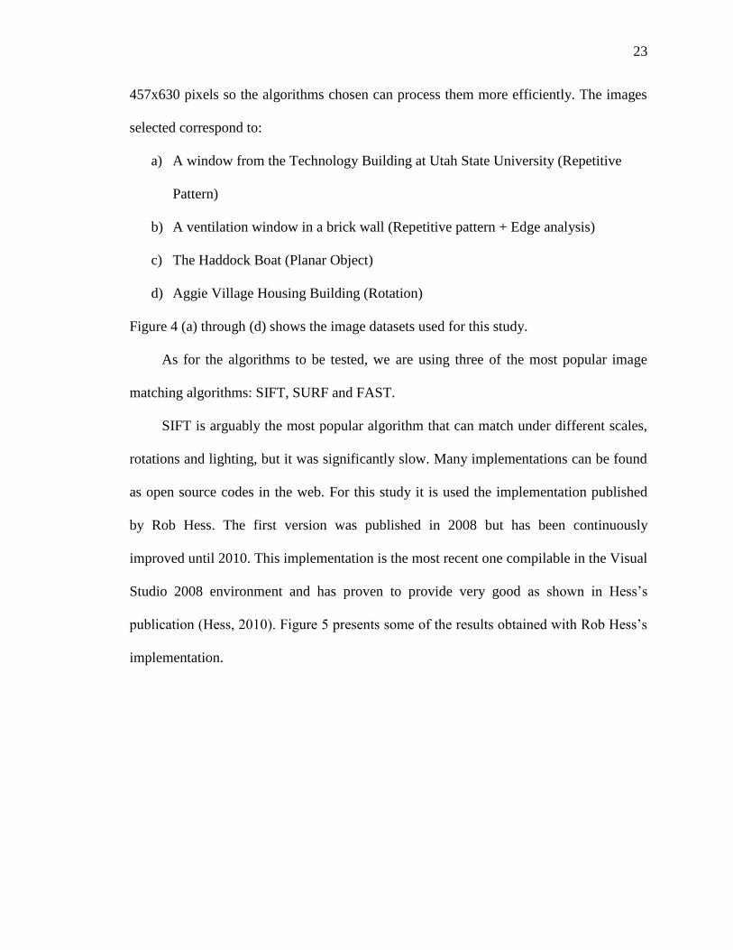
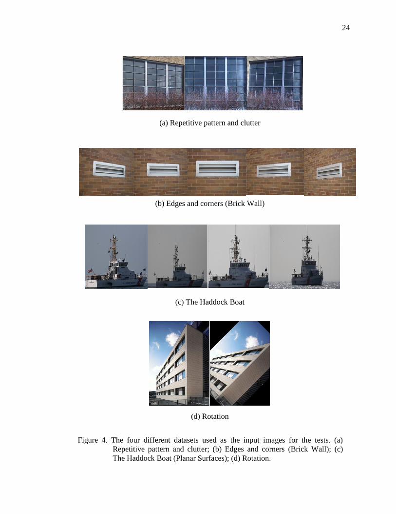
457x630 pixels so the algorithms chosen can process them more efficiently. The images
selected correspond to:
a) A window from the Technology Building at Utah State University (Repetitive
Pattern)
b) A ventilation window in a brick wall (Repetitive pattern + Edge analysis)
c) The Haddock Boat (Planar Object)
d) Aggie Village Housing Building (Rotation)
Figure 4 (a) through (d) shows the image datasets used for this study.
As for the algorithms to be tested, we are using three of the most popular image
matching algorithms: SIFT, SURF and FAST.
SIFT is arguably the most popular algorithm that can match under different scales,
rotations and lighting, but it was significantly slow. Many implementations can be found
as open source codes in the web. For this study it is used the implementation published
by Rob Hess. The first version was published in 2008 but has been continuously
improved until 2010. This implementation is the most recent one compilable in the Visual
Studio 2008 environment and has proven to provide very good as shown in Hess‟s
publication (Hess, 2010). Figure 5 presents some of the results obtained with Rob Hess‟s
implementation.
24
(a) Repetitive pattern and clutter
(b) Edges and corners (Brick Wall)
(c) The Haddock Boat
(d) Rotation
Figure 4. The four different datasets used as the input images for the tests. (a)
Repetitive pattern and clutter; (b) Edges and corners (Brick Wall); (c)
The Haddock Boat (Planar Surfaces); (d) Rotation.

25
SURF was published after SIFT and it was intended to overcome the computational
cost derived from using this latter and also the amount of time consumed by the
algorithm. The SURF implementation used in this study was developed by Christopher
Evans in 2008 and has been continuously improved and revised up to May 2010. He also
wrote the paper “Notes on the Open SURF Library” where is explained in detail the
analysis of the Speeded-Up Robust Features computer vision algorithm along with a
breakdown of the Open-SURF implementation. It also contains useful information on
machine vision and image processing in general (Evans, 2008). This library is available
in two versions: C++ and C#. The C++ version comes with the image matching
component whereas the C# only has the feature detection component. Both the C++ and
C# implementations are used in this study.
Figure 5. Results presented by Rob Hess with the implementation of the SIFT algorithm
for object recognition. Top: SIFT features detected in two images. Bottom: SIFT
featured matches between the two images.

26
FAST is the only feature-based algorithm from the three used for this study. It was
first developed by Trajkovic and Hedley in 1998. The implementation used was
published by Edward Rosten (Rosten and Drummond, 2009) as well. All of these
implementations utilize the OpenCV library of programming functions for real time
computer vision.
3.3 Experimental Process
The images shown above will be tested with each algorithm and these, in turn, will
be tested in different categories having as a final and principal goal the assessment of the
intrinsic algorithm characteristics that will make it differ from another. Robustness,
speed, number of features and number of matches are some of the parameters that will be
evaluated. Due the nature of this research we need to ensure the applicability of its results
to almost any derivate circumstance in which a comparative study image vs. algorithm
performance may become handy. After the data have been chosen, we will undertake an
Figure 6. FAST corner detection demonstration.

27
experimental process that is expected to reveal the effectiveness of the algorithms for
different sets of images.
The methodology to be followed is broken down into the following steps.
3.3.1 Data selection
The images selected were described and presented in section 3.2. Each of these
datasets recreates one or more of the conditions that commonly affect images and that
constitute a challenge for the matching algorithms.
3.3.2 Image pairs
The images used in this study will be taken in pairs with a difference in orientation
no greater than 30° from one image to its matching pair. Some of the algorithms used in
this study are unable to handle images with high pixel resolution (i. e. N x M pixel size
greater or equal to 1 MP). Due to this, the images taken were cropped and resized to the
maximum sizes that SIFT, SURF and FAST could efficiently process. The size used for
this work is 457x630 pixels. The selection of the image pairs that were tested depended
on the parameters that are more significant to our purposes. It is necessary to ensure that
the image pairs selected represent at least one of the parameters mentioned in section 1.1.
The image pairs are shown in Figures 7-10.
3.3.3 Feature detection
After the images pairs are selected, the feature detection component of each
algorithm was run over the image pairs. SIFT, SURF and FAST all are coded to perform
feature detection first. The purpose of this run is to quantify the difference between the
numbers of features detected by the algorithms and also the “quality” of these features.

28
Figure 7. Windows (First Pair).
Figure 8. Brick Wall (Second Pair).

29
Figure 9. The Boat (Third Pair).
Figure 10. The building (Fourth Pair).

30
3.3.4 Manual detection of matches candidates
The amount of features detected is not a measure of a „good‟ performance by itself.
Better than detecting 100 features is detecting 100 important features in the image.
Certain parts of the image contain more information than others and these are the one that
will have a higher chance of finding a match candidate. A visual inspection of the
features detected with SIFT, FAST and SURF was performed. A total of 20 features were
manually matched at each of the image pairs (please refer to Appendix E for manual
matching on image pairs). Each pair of feature detected as a match was connected to
each other with a straight line, as shown in Appendix E. The process was made for each
image pair and each algorithm. FAST is the only one of the three algorithms tested that
does not have a matching component available as an open code. The features detected
with FAST in each image pair were manually matched to determine the amount of
features from image A of the pair that has a correspondent feature on Image B. Although
this could be somehow „unfair‟ for the other algorithms, because a manual match closely
compares to a „perfect‟ model, a proportionality analysis can be performed to truly assess
the behavior of the three algorithms as fair as possible.
3.3.5 Automated detection of matching
After the manual matching process was completed for each algorithm, the matching
component of SIFT and SURF was run. This allowed the algorithms to automatically find
the matches from the feature points previously detected.

31
3.3.6 Evaluating the results
The results obtained from the previous steps were assessed in terms of the number
of errors incurred in the detection of accurate matches by the algorithms. As a measure of
the success, the errors will be classified utilizing the Type I and Type II error method.
Type I error occurs when real matches are not detected by the algorithms. In this case
having the algorithm found the same feature point on both images composing the pair; it
does not recognize them as a match in the subsequent step. A Type II error is generated
when the algorithm mismatches a feature. Typically, mismatches or false negative can be
visually identified as crossing lines draw between the matches. This is further explained
in Chapter 4.
Type I errors were computed by determining the number of matches that the
algorithm failed to identify as matches from the ones manually detected in section 3.3.4.
We want the number of type I errors to be low because a high number of type I errors
reflect failures in the algorithm to accurately detect matches. For image matching
algorithms we want the number of type II errors found to be low also. A high number of
type II errors are a measure of inaccuracy in the algorithm because it is mismatching
features within the pair.
3.3.7 Final comparison
After all the results have been collected and analyzed in depth, a comparison
between the statistical values derived from the results of each method is evaluated. From
this, the conclusions of this research will be shaped.

32
CHAPTER 4
DATA ANALYSIS
This chapter describes the step by step implementation of the methodology
proposed. Some considerations and exceptions had to be made in some cases and these
changes are also explained herein.
4.1 Feature Detection
4.1.1 SIFT feature detection
Figure 11. SIFT feature detection algorithm.
33
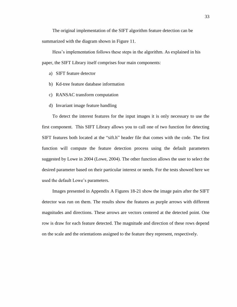
The original implementation of the SIFT algorithm feature detection can be
summarized with the diagram shown in Figure 11.
Hess‟s implementation follows these steps in the algorithm. As explained in his
paper, the SIFT Library itself comprises four main components:
a) SIFT feature detector
b) Kd-tree feature database information
c) RANSAC transform computation
d) Invariant image feature handling
To detect the interest features for the input images it is only necessary to use the
first component. This SIFT Library allows you to call one of two function for detecting
SIFT features both located at the “sift.h” header file that comes with the code. The first
function will compute the feature detection process using the default parameters
suggested by Lowe in 2004 (Lowe, 2004). The other function allows the user to select the
desired parameter based on their particular interest or needs. For the tests showed here we
used the default Lowe‟s parameters.
Images presented in Appendix A Figures 18-21 show the image pairs after the SIFT
detector was run on them. The results show the features as purple arrows with different
magnitudes and directions. These arrows are vectors centered at the detected point. One
row is draw for each feature detected. The magnitude and direction of these rows depend
on the scale and the orientations assigned to the feature they represent, respectively.

34
4.1.2 SURF feature detection
The OpenSURF Library is very similar to the SIFT Library when it comes to
feature detection. The main difference relies on the use of an integral image from the first
as the basis for this detection. The use of a very basic Hessian-matrix approximation
facilitates the implementation of the integral image concept which in turn speeds up the
detection. The detector is based on the Hessian matrix because of its good performance in
accuracy. More precisely, the algorithm detects blob-like structures at locations where the
determinant of this matrix is maximum (Bay et al., 2006).
One important reason to implement this feature extraction method is because it
provides complementary information about the region of interest that cannot be obtained
from edge or corner detectors. Also, the improvement on speed achieved with this
implementation is a very desirable factor for many processes. The OpenSURF Library
used in this study follows the steps described above (Evans, 2008).
This algorithm draws the features as ellipses of different sizes and colors. The size
of each ellipse is governed by the function (g.DrawEllipse(Pen pen, int x, int y,
int width, int height). This function takes the x and y values from the coordinates
of the feature detected. The width and height parameters have the same value and are
denoted by the variable S. Width and height are both factors of the feature scale. Their
computation is achieved by using the following relation:
Features are also colored blue or red on dependence of value of the Laplacian
matrix. If the Laplacian value of a particular point is greater than 0, then the ellipse will
int S = 2 * Convert.ToInt32(2.5f * ip.scale);
(1)

35
be blue colored, otherwise, the resultant ellipse will be draw in red (please refer to
Appendix A Figures 22-25). This is achieved by applying the following statement:
The reason why the sign of the Laplacian is important for feature detection is
explained in the next lines extracted from the notes on the OpenSURF Library (Evans,
2008):
SURF detector is based on the determinant of the Hessian matrix. In order to
motivate the use of the Hessian, we consider a continuous function of two variables
such that the value of the function at (x; y) is given by f(x; y). The Hessian matrix,
H, is the matrix of partial derivates of the function f.
The determinant of this matrix, known as the discriminant, is calculated by:
The value of the discriminant is used to classify the maxima and minima of
the function y the second order derivative test. Since the determinant is the product
of eigenvalues of the Hessian we can classify the points based on the sign of the
result. If the determinant is negative then the eigenvalues have different signs and
hence the point is not a local extremum; if it is positive then either both eigenvalues
are positive or both are negative and in either case the point is classified as an
extremum.
myPen = (ip.laplacian > 0 ? bluePen :
redPen);
(2)
(3)
(4)

36
4.1.3 FAST feature detection
As mentioned previously, FAST is the only feature-based algorithm from the three
presented in this work. Because of this difference the process through which FAST
detects feature points varies significantly from SIFT and SURF. FAST relies on a corner
response function (CRF) to robustly detect corners in a given scene. It also used a
multigrid algorithm to detect corners that speeds the process significantly (Trajkovic and
Hedley, 1998). The three-step multigrid algorithm used to detect comers is presented
below.
Step 1: In a low resolution image, compute the simple CRF at every pixel location.
Classify pixels with a response higher than a define threshold T1 as „potential
corners‟.
Step 2: Using the full resolution image for each potential corner pixel, compute the CRF.
If the response is lower than another threshold already detected, then the pixel is
not a corner, and the upcoming step is not performed. If not, use a interpixel
approximation and compute a new response. If the response is lower than the
second threshold T2 then the pixel is not a comer.
Step 3: Find pixels with a locally maximal CRF and mark them as corners. This step is
necessary since in the vicinity of a corner more than one point will have high
CRF, and only the largest CRF is declared to be a comer point. This is called non-
maximum suppression (NMS).
Features detected with FAST are drawn as blue circles on the input image. The
center of the circle is located at the x and y coordinates of the feature detected. These
circles have a fixed radius and thickness of 5 and 1 P respectively. Refer to Appendix A

37
Figures 26-29 for the FAST feature detection results on the image pairs used for this
study.
4.2 Feature Matching
4.2.1 SIFT feature matching
The feature matching process is done through the match.c function in the SIFT
Library. This function is explained in as follows (Hess, 2010):
match.c: This application computes matches between SIFT key points detected in
two images using the library's kd-tree functions and optionally computes a transform
based on those matches using the library's RANSAC functions.
This is again, a matching application of the SIFT algorithm that correspond very
similarly to the one described by David Lowe in his 2004 publication. The results
obtained with this SIFT Library and the original are very comparable as shown in Table
2.
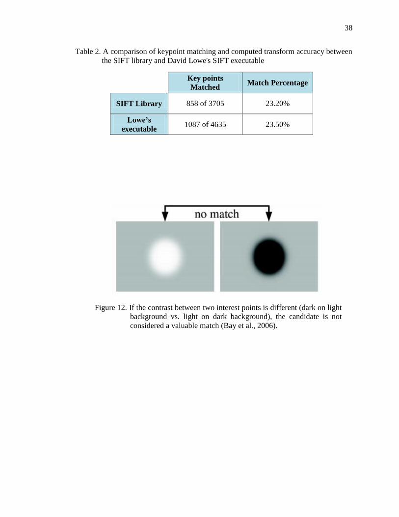
4.2.2 SURF feature matching
SURF uses an indexing process to accelerate the matching stage. As explained
before, typically the interest feature points are derived from blob structures and this,
along with the sign of the Laplacian obtained during the detection step distinguishes
bright blobs on dark backgrounds from the reverse situation (Bay et al., 2006). In the
matching stage, it only compare features if they have the same type of contrast, see
Figure 12. Hence, this minimal information allows for faster matching, without reducing
the descriptor's performance.
38
Table 2. A comparison of keypoint matching and computed transform accuracy between
the SIFT library and David Lowe's SIFT executable
Key points
Matched Match Percentage
SIFT Library 858 of 3705 23.20%
Lowe’s
executable 1087 of 4635 23.50%
Figure 12. If the contrast between two interest points is different (dark on light
background vs. light on dark background), the candidate is not
considered a valuable match (Bay et al., 2006).

39
4.2.3 FAST feature matching
FAST matching component is not yet available as an open source code. Therefore,
the automatic detection of matches could not be used in this study. However, a manual
detection of the matches as explained in the third step of the experimental process. The
results of this analysis and how are these results comparable with the automated matches
from SIFT and SURF is detailed in Chapter 5.

40
CHAPTER 5
RESULTS AND CONCLUSIONS
5.1 General Overview
The experimental process followed up for this study yielded some expected results.
One important consideration is that the image dataset used consists of images that
represent typical cross-sections of scenes in the real world. The image size was modified
to allow quick and efficient performance from the algorithms. Table 3 summarizes the
number of features detected by each algorithm for a given pair of images.
5.2 Feature Detection Results
While implementing the feature detection component on the images it was found
that despite the image, SIFT detects more features than FAST or SURF. The results of
this feature detection process are shown in Figures 13 to 16. Given SIFT is a proven
robust feature detector, it comes as no surprise the high amount of features detected in the
images as shown in Appendix A Figures 18-21. The images present a high number of
features detected by SIFT and these are presented by purple arrows (see section 4.1.1).
However, in the majority of the images, SIFT detected features at places that did not
seem to contain enough information for later matching. Corners, edges, highly
contrasting, and important parts of the objects are considered good features. In the
Windows pair for example (Figure 19, Appendix A), SIFT detected a lot of features in
the bottom part where some tree branches are but did not detect stronger parts of the
image such as corners on the window, edges, etc. Similarly, in the Brick Wall pair

41
(Figure 20, Appendix A) a lot of futures were detected in places that do not contain
enough information. However, SIFT does detects good features in some cases. In the boat
image pair for example (Figure 20, Appendix A), a lot of strong points on the boat were
detected as features, but again, it can be appreciated that some features were detected in
the air which doesn‟t seem to be a good key point candidate.
SURF follows SIFT in the amount of features detected but the difference is
considerable between both for the majority of the images. SURF, although finding less,
detected more “robust” features (i.e. features with enough information for later match). If
we compare the results of the features detected with SURF in the Window image pair
(Figure 22, Appendix A) with those detected with SIFT on the same pair, it can be seen
that SURF features are mostly detected on the edges of the windows. This is a good
indication of the algorithm performance, because it is selecting features that are very
likely to be matched. In the brick wall pair (Figure 23, Appendix A), SURF detected
features along the edges of the ventilation window. Although with some missing parts
and weak features detected the overall performance of SURF detector can be described as
better than SIFT for most of the images.
FAST on the other hand found very few features in all of the images tested. Given
FAST is a feature-based detector, one could expect a higher amount of detections. But
corner detectors usually limit themselves to detect pixels in the image with high contrast
and rejected any other. Although features with more information are more desirable, this
seemed to harm the performance of FAST in the quantitative aspect, but the quality of the
features is undoubtedly among the best.

42
If we analyze the results obtain with FAST in the Window image pairs (Figure 26,
Appendix A) with the results obtained with SIFT and SURF we can appreciate the
robustness of FAST features over the others. These features majorly detected on the
corners of the windows. FAST is not flawless, some weak features were also detected at
the bottom of the Window pair. In the Brick Wall images pair (Figure 27, Appendix A),
FAST did not find as much features as one would expect. This is presumably due to the
lack of high contrast and poor illumination at the edges of the bricks. But FAST detected
three of the four corners on the ventilation window.
Having discussed the results of the feature detection part of this study, one can say
that the amount of features by itself should not be taken as measure of the effectiveness
of the algorithm. It is important to determine first, how many of those features are
actually robust enough to survive further filtering steps and become a positive match.
Table 3. Number of feature detected in the image dataset for the three algorithms
Features Detected
Pair Image SIFT SURF FAST
Window Pair A 859 770 86
B 754 734 128
Brick Wall
Pair
A 1117 507 13
B 1106 516 6
Boat Pair A 484 209 50
B 604 326 294
Building Pair A 842 606 216
B 550 202 52

43
0
200
400
600
800
1000
1200
A B
# o
f fe
atu
res
Images
Features Detected-Second Pair
SIFT
SURF
FAST
0
100
200
300
400
500
600
700
800
900
1000
A B
# o
f fe
atu
res
Images
Features detected-First Pair
SIFT
SURF
FAST
Figure 13. Features detected in the Window image pair (Images A and B).
Figure 14. Features detected in the Brick Wall Image pair (Images A and B).

44
0
100
200
300
400
500
600
700
A B
# o
f fe
atu
res
Images
Features detected-Third Pair
SIFT
SURF
FAST
0
100
200
300
400
500
600
700
800
900
A B
# o
f fe
atu
res
Images
Features detected-Fourth Pair
SIFT
SURF
FAST
Figure 15. Features detected in the Boat Image pair (Images A and B).
Figure 16. Features detected in the Building Image pair (Images A and B).
45
Let‟s discuss the performance of each algorithm for a given type of images. The
results of this are presented in the Figure 17.
a) SIFT detected the most feature points on image No. 3. This image corresponds to
the first view of the brick wall pair. This was expected because of the large
amount of texture of this image (visually appreciated). On the other hand, SIFT
had the lowest detection with image 5 corresponding to the first view of the
Haddock Boat. This also confirm the hypothesis of SIFT performing at the
highest levels when tested on textured images. This can be also checked by
looking at the results for the other images.
b) SURF is also a textured based matching algorithm but it seemed to get confused
in textured images with illumination changes (as is the case with the brick wall
pair). Because of this, it did not have its best performance with this pair. The
image with most features detected by SURF was the corresponding second one
for SIFT: The window image pair (Figure 22, Appendix A). The less feature
detection occurred again in the pair corresponding to the boat (Figure 24,
Appendix A). This proves that SIFTS and SURF being texture-based algorithms,
do not perform well when tested on planar images.
c) FAST, conversely to SIFT and SURF, detected more features in the pair
comprised by the Haddock boat. Although in general the amount of features
detected by FAST are significantly less than SIFT or SURF, it is appreciated that
the best performance of this type of algorithms (feature-based) will be enhanced if
the appropriate set of image is selected. And as explained before, FAST found the
fewer amount of features in the Brick Wall image pair (Figure 27, Appendix A).

46
0
200
400
600
800
1000
1200
1 2 3 4 5 6 7 8
# o
f fe
atu
res
Images
Features Detected
SIFT
SURF
FAST
This is an unexpected result from FAST due to the large number of corners and
edges within this image, but this is presumably because of the low contrast and
poor illumination at the corners and edges of the brick.
The results presented in Figure 17 provide evidence that how these two types of
algorithms perform is dependent on the type of image used.
Image 1 and 2: First and second views of the Window Pair, respectively.
Image 3 and 4: First and second views of the Brick Wall Pair, respectively.
Image 5 and 6: First and second views of the Boat Pair, respectively.
Image 7 and 8: First and second views of the Building Pair, respectively.
Figure 17. Overall view of the features detected on each image.

47
5.3 Feature Matching Results
The reason why accurate feature detection is so important is to facilitate matching.
In this step, all the features detected in one image are tested one by one against the entire
database holding all the values from all the features detected in the second image to find
one containing the same information. When the same information is found then a new
match is originated. However, sometimes these algorithms fail to detect simple matches.
In order to measure the effectiveness and accuracy of the matching process on both
SIFT and SURF algorithms, the steps described in the methodology, section 3.3, were
followed. First, we created a truth dataset by taking the features detected by the algorithm
and manually matching the features that that were expected the algorithm to identify as
matches. For this part of the experiment we manually detected potential matches for the
three algorithms. It is important to note that the source code for the matching component
of FAST is not available and therefore does not take part in the detection of type II errors.
The reason why the manual matches were also performed for FAST is because if this
algorithm proves to be highly accurate in the detecting the same features on both images,
the feature work in developing the matching component could be recommended.
The images showing the manual matches detection for SIFT, SURF and FAST can
be found in Appendix D.
The following is a discussion of the algorithms matching performances for each
pair of images:
SIFT: Having consistently detected more features than SURF and FAST, SIFT was,
as expected, the algorithm with more matches found for each image pair. SIFT detected a
maximum total of 203 matches in the Building Image pair. The lowest matches for SIFT

48
correspond to the Windows pair with a total of 17. The pair with the Haddock boat had a
total of 23 matches detected. Table 4 summarizes these results and gives a percentage of
efficient based on the amount of matches found put of the totality of the features detected
by SIFT.
SURF: Again, it follows SIFT in the amount of matches found among the images,
proving that the amount of features detected is indeed proportional to the amount of
matches. SURF had the highest matches at the Building pair, as SIFT. And the lowest
detection in the third pair which is the Haddock boat pair.
FAST: As explained before, FAST does not have an automated matching
component, and therefore the matches were manually identify in order to quantify the
amount of features that are accurately detected in both images of the pair. The less
matches were manually detected in the second image pair, the brick wall, and the most at
the Building pair. However, this cannot be taken as a final conclusion because it is
necessary to measure the efficiency of the matches rather than the quantity of these.
Tables 4 to 6 present the number of matches detected by each algorithm for a given
pair. The effectiveness of this process is also presented. The effectiveness was calculated
using the following relation:
%𝐸𝑓𝑓𝑒𝑐𝑡𝑖𝑣𝑒𝑛𝑒𝑠𝑠 =2∗#𝑚𝑎𝑡𝑐 ℎ𝑒𝑠
#𝑓𝑒𝑎𝑡𝑢𝑟𝑒𝑠 (5)
By looking at the results, it can be seen that the number of matches is very low in
comparison with the amount of features detected. Knowing this, we can conclude that the
number of matches by itself cannot be considered good. We need to compare that amount
with the amount of features detected to see how many of those features is the algorithm

49
actually using. Automated matching from SIFT and SURF are presented in tables 4 and
5. FAST manually matching is presented in table 6. Unfortunately, the manual matching
that was made for FAST cannot be compared with the automated matches from SIFT and
SURF without giving an artificial conclusion. However, the results obtained with these
manual matches prove that FAST detects more robust features than SIFT and SURF and
that therefore are more likely to derive good matches. This is discussed in further detail in
section 5.4.
Table 4. Matching performance for SIFT
SIFT
Features # Matches % Effectiveness
Window
Pair
859 17 2%
754
Brick
Wall Pair
1177 113 10%
1106
Boat Pair 484
23 4% 604
Building
Pair
842 203 29%
550
Table 5. Matching performance for SURF
SURF
Features # Matches % Effectiveness
Window
Pair
770 24 3%
734
Brick Wall
Pair
507 72 14%
516
Boat Pair 209
10 4% 326
Building
Pair
606 102 25%
202

50
Table 6. Matching performance for FAST
More important than the amount of matches, is the quality of these matches.
Another analysis that was undertaken to determine the quality of the matches was to
measure the accuracy of each of the matches. In order to do this, the matching component
of the algorithms was run and allowed to automatically detect matches. Once the matches
were automatically detected, the accuracy of the matches was visually analyzed and
compared with the manual matches done early (see section 3.3.4). For every match from
the 20 manually detected that the algorithm missed a type I error was counted. The
matching process depends on the feature detection. And it is expected for a good
matching algorithm to detect all the matches that can be visually or manually detected. If
the algorithm does not detect those manual matches, it can be said that the matching
component of such algorithm does not perform as good as it should. On the other hand,
every mismatch was counted as a type II error (matching two features without being a
match in the image pair). The amount of type II errors is, for this study, a more important
parameter than the amount of type I. Type I errors reflect weakness in the algorithm in
FAST
Features # Matches % Effectiveness
Window
Pair
86 17 16%
128
Brick Wall
Pair
13 5 53%
6
Boat Pair 50
18 10% 294
Building
Pair
216 26 19%
52

51
detecting all the matches. Type II errors reflect a failure in the algorithm for matching
features without being conjugate points.
In Appendix B the automated matches detected for each pair are shown. Note that
for the Brick Wall and the Building pair, SIFT and SURF again found a very large
amount of matches. Therefore, it was decided to limit the number of matches detected, to
make the manual error detection easier. The matches were restricted to about the same
number by modifying the thresholds values. Appendix C has the matches after the
parameters were modified to restrict the amount detected. The computation of type I and
type II errors for SIFT and SURF is summarized in tables 7 and 8, respectively.
By comparing these two algorithms in terms of the amount of type I and type II
errors it is obvious that SIFT incurred, in proportion, more errors than SURF. The large
number of features detected with SIFT are not as good as those detected with SURF and
because of this, it fails to match them. It is important to keep in mind that with this
analysis we are not comparing the type of images that are most suitable for one algorithm
or the other, because both SIFT and SURF are texture based algorithms and were proven
to work similarly on the same images. With that clarified, it can be stated that in general,
the features detected by these texture algorithms will not provide features good enough to
accurately extract objects from a given images. Mainly because of the amount of features
detected in insignificant areas of the images (this can be visually checked with the images
in Appendix A).

52
Table 7. Type I and Type II errors detection for SIFT matches
SIFT
Pair # Matches Type
I
Type
II Type I % Type II %
Window 17 12 14 60% 82%
Brick Wall 53 11 7 55% 13%
Boat 75 8 5 40% 7%
Building 23 4 10 20% 43%
Table 8. Type I and Type II errors detection for SURF matches
5.4 Conclusions
After reviewing the results obtained in this research we can conclude the following:
a) The amount of features detected by SIFT, FAST and SURF is dependent on the
type of images used.
b) SIFT and SURF, as texture-based detectors, were found to detect more features
when highly texture images were used.
SURF
Pair # Matches Type
I
Type
II
Type I
%
Type II
%
Window 24 5 13 25% 54%
Brick Wall 51 9 14 45% 27%
Boat 10 2 0 10% 0%
Building 74 0 9 0% 12%

53
c) FAST on the other hand, performed more accurately where SIFT and SURF
“failed”. This means that FAST, being a feature-based algorithm, will perform
better in when tested to images containing planar objects.
d) The amount of features is not a measure of success by itself but the “quality” of
these features
e) The amount of features detected is proportional to the amount of matches.
f) SIFT was the algorithm detecting more features and matches in all the images.
g) The amount of matches detected is not a good indication of the performance of
the algorithm
h) SIFT found more matches than SURF and FAST but also less effectiveness was
measured
i) The effectiveness ratios were not as promising as the amount of matches.
Furthermore, the amounts of type I and II errors encountered in both SIFT and
SURF determined that these two algorithms need to be improved to reject some
useless features and detect more robust ones.
j) FAST detected considerably less matches than SIFT but it had a better
performance, proportionally.
k) Features detected by FAST, although fewer, are more robust than those detected
by SIFT and SURF.
54
CHAPTER 6
RECOMMENDATIONS
A comparative study of three image matching algorithms has been done in this
research. Results obtained proved that the hypothesis that the performance of a given
algorithm depends on the type of image used is true. Visually textured and non-textured
images were used to prove this. It is recommended for future research in this area to use a
method to statistically evaluate the texture of the images such as the maximum entropy
method. These methods use statistical analysis to measure the parts of the images with
more information and develop a model of the texture of the image base on this.
It was concluded that FAST has the best overall performance above SIFT and
SURF but it suffers from detecting very few features and therefore matches. It is
recommended that the properties of this algorithm to be improved by creating a new
implementation provided with a matching component. It is necessary to improve FAST
by increasing the amount of features it can detect. But special care should be taken to
preserve the robustness of the algorithm and avoid the detection of useless features.
Future research in this area should focus on testing the accuracy of the algorithms in
detecting a single object within a scene. Many of the new arising needs in
photogrammetry address this problem and this work could be a first step towards a more
in depth study.
The results reported in this work are likely a starting point for future research on
this subject where a more in-depth analysis of the algorithms structures would be done.
Also, an automated assessment of the algorithms performance could follow where future

55
researches would be able to consider a wider range of issues that need to be addressed
when working with SIFT, SURF, and FAST.

56
REFERENCES
Babbar, G., Punam Bajaj, Anu Chawla, and Monika Gogna. 2010. A comparative study
of image matching algorithms. International Journal of Information, Technology
and Knowledge Management. July-December. 2(2): 337-339.
Barazzetti, L., F. Remondino, and M. Scaioni. 2010. Extraction of accurate tie points for
automated pose estimation of close-range blocks. IAPRS, Vol. XXXVIII, Part 3A
– Saint-Mandé, France, Septiembre 1-3, 2010.
Bay, H., A. Ess, T. Tuytelaars, and L. Van Gool. 2006. Speeded-up robust features
(SURF). Computer Vision ECCV 2006, Vol. 3951. Lecture Notes in Computer
Science. p. 404-417.
Barrow, E.A., J.M. Tenenbaum, R.C Bolles, and H.C. Wolf. 1977. Parametric
correspondence and chamfer matching: Two new techniques for image matching.
SRI International (5):659-667.
Dorkó, G., and C. Schmid. 2003. Selection of scale-Invariant parts for object class
recognition. Proceedings on Ninth IEEE International Conference on Computer
Vision 2003, 13-16 Oct. 2003, Nice, France.
Evans, C. 2008. Notes on the OpenSURF library. UK Publication Papers. Issue 1,
Citeseer. p. 25.
Fraser, C., I. Jazayeri, and S. Cronk. 2010. A feature-based matching strategy for
automated 3D model reconstruction in multi-Image Close-Range
Photogrammetry. ASPRS 2010 Annual Conference, April 26-30, 2010, San
Diego, California.
Harris, C. 1988. A combined corner and edge detector. Fourth Alvey Vision Conference,
Manchester, UK. p. 147-151.
Hess, R. 2010. An open source SIFT library. Proceedings of the International Conference
in Multimedia, 2010, Firenze, Italy. p. 1493-1496.
Hoiem, D., N. Andrew, A. Stein, A. Alexei and, M. Hebert. 2007. Recovering occlusion
boundaries from a single image. IEEE 11th
International Conference on Computer
Vision, 2007. p. 1-8.
Juan, L., and O. Gwun. 2009. A comparison of SIFT, PCA-SIFT, and SURF.
International Journal of Image Processing (IJIP) 3(4): 143-152.

57
Kanade, T., and M. Okutomi. 1994. A stereo matching algorithm with and adaptive
window: Theory and experiment. IEEE Transactions on Pattern Analysis and
Machine Intelligence, September 1994, (TPAMI) 16: 920-932.
Ke, Y., and R. Sukthankar. 2004. PCA-SIFT: A more distinctive representation for local
image descriptors. IEEE Computer Society Conference on Computer Vision and
Pattern Recognition (CVPR'04) – 2: 506-513.
Lowe, D.G. 1999. Object recognition from local scale-invariant features.The proceedidng
of the seventh IEEE International Conference on Computer Vision 1999. 2: 1150-
1157.
Lowe, D.G. 2004. Distintive image feature from scale-invariant keypoints. International
Journal of Computer Vision, 60(2): 91-110.
Mikolajczyk, K, and. C. Schmid. 2004. Scale and affine invariant interest point
detectors. International Journal of Computer Vision 60(1): 63-86.
Rosenholm, D. 1987. Least squares matching method: Some experimental results. The
Photogrammetric Record 12(70): 493-512.
Rosten, E., and T. Drummond. 2006. Machine learning for high-speed corner detection,
IEEE Trans. Pattern Analysis and Machine Intelligence 2006. p. 430-443.
Schenk, T., A. Krupnik, and Y. Postolov. 2000. Comparative study of surface matching
algorithms. International Archives of Photogrammetry and Remote Sensing Vol.
XXXIII, part 4B, Amsterdam 2000. p. 518-524.
Smith, S. M., and J. M. Brady. 1997. SUSAN A new approach to low level image
processing. International Journal of Computer Vision 23(1): 45-78.
Trajkovic, M. and M. Hedley. 1998. FAST corner detector. Image and Vision Computing
16: 75-87.
Wang, H., and M. Brady. 1994. A practical solution to corner detection. Proceedings in
IEEE International Conference of Image Processing 1994, ICIP-94. 13-16
November 2004, Austin, Texas. 1: 919-923.
Wallis, K. F. 1974. Seasonal adjustment and relations between variables. Journal of the
American Statistical Association. 69(345): 18-31.

58
APPENDICES

59
Appendix A. Feature Detection Images
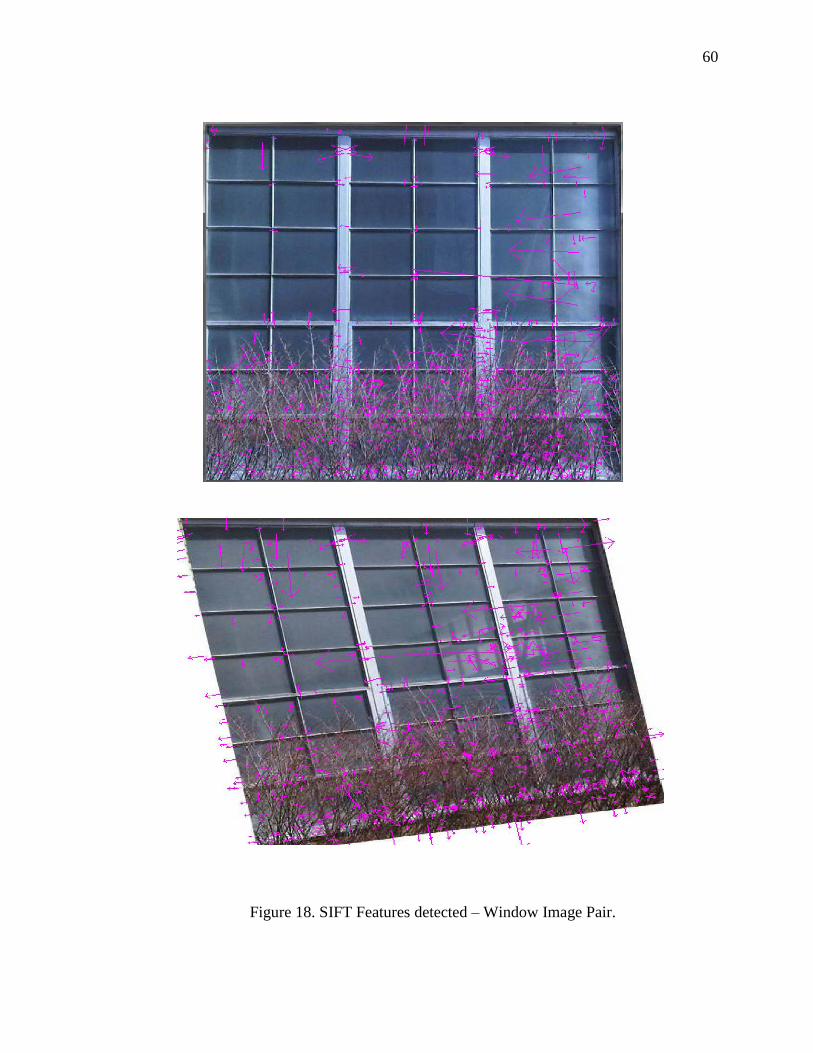
60
Figure 18. SIFT Features detected – Window Image Pair.

61
Figure 19. SIFT Features detected – Brick Wall Image Pair.

62
Figure 20. SIFT features detected – Boat Image Pair.

63
Figure 21. SIFT Features detected – Building
Image Pair.
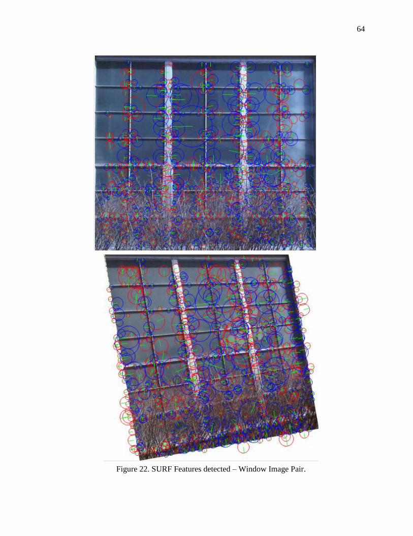
64
Figure 22. SURF Features detected – Window Image Pair.

65
Figure 23. SURF Features detected – Brick Wall Image Pair.

66
Figure 24. SURF Features – Boat Image Pair.

67
Figure 25. SURF Features detected –
Building Image Pair.

68
Figure 26. FAST Features detected – Window Image Pair.

69
Figure 27. FAST Features detected – Brick Wall Image Pair.

70
Figure 28. FAST Features detected – Boat Image Pair.

71
Figure 29. FAST Features detected – Building Image Pair.

72
Appendix B. Matches

73
Figure 30. SIFT Matches – Window Image Pair.

74
Figure 31. SIFT Matches – Brick Image Pair.

75
Figure 32. SIFT Matches – Boat Image Pair.

76
Figure 33. SIFT Matches – Building Image Pair.

77
Figure 34. SURF Matches – Window Image Pair.

78
Figure 35. SURF Matches – Brick Wall Image Pair.

79
Figure 36. SURF Features for third pair – Boat Image Pair.

80
Figure 37. SURF Matches – Building Image Pair.

81
Appendix C. Matches found after threshold modification
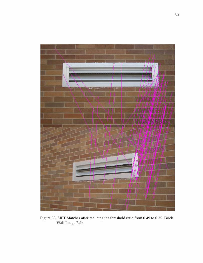
82
Figure 38. SIFT Matches after reducing the threshold ratio from 0.49 to 0.35. Brick
Wall Image Pair.

83
Figure 39. SIFT Matches after reducing the threshold ratio from 0.49 to
0.35. Brick Wall and Building Image Pairs.
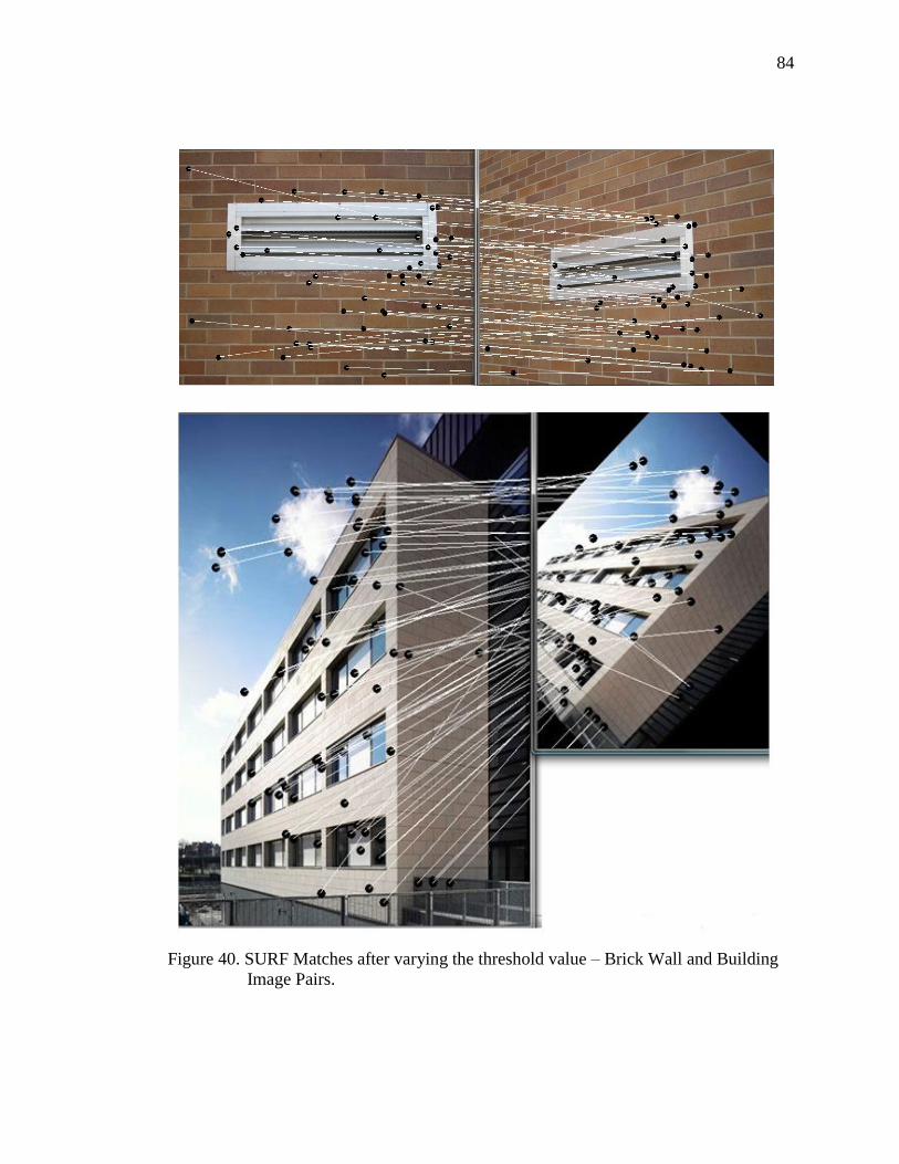
84
Figure 40. SURF Matches after varying the threshold value – Brick Wall and Building
Image Pairs.

85
Appendix D. Type II error detection (Mismatches)

86
Figure 41. SIFT incorrect matches – Window Image Pair.

87
Figure 42. SIFT Incorrect Matches – Brick Wall Image Pair.

88
Figure 43. SIFT incorrect matches – Boat Image Pair.

89
Figure 44. SIFT incorrect matches - Building Image Pair.

90
Figure 45. SURF incorrect matches – Window Image Pair.

91
Figure 46. SURF incorrect matches – Brick Wall Image Pair.

92
Figure 47. SURF incorrect matches – Boat Image Pair.

93
Figure 48. SURF incorrect matches – Building Image Pair.

94
Appendix E. Manual matching for detected features

95
Figure 49. Manually detected potential matches for SIFT – Window Image Pair.
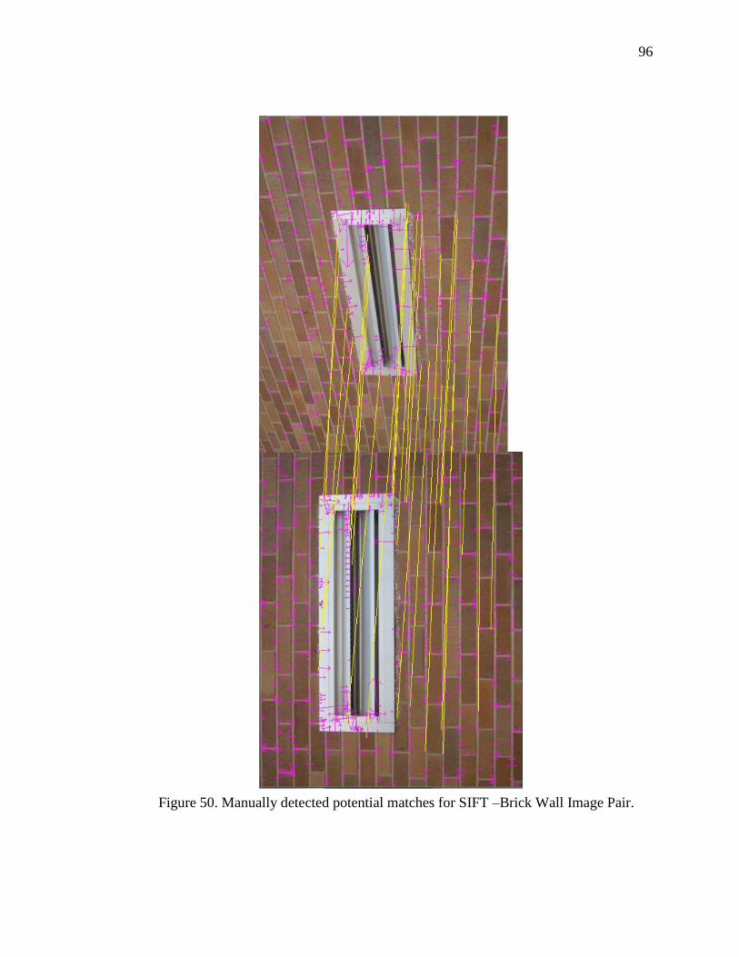
96
Figure 50. Manually detected potential matches for SIFT –Brick Wall Image Pair.

97
Figure 51. Manually detected potential matches for SIFT –Boat Image pair.
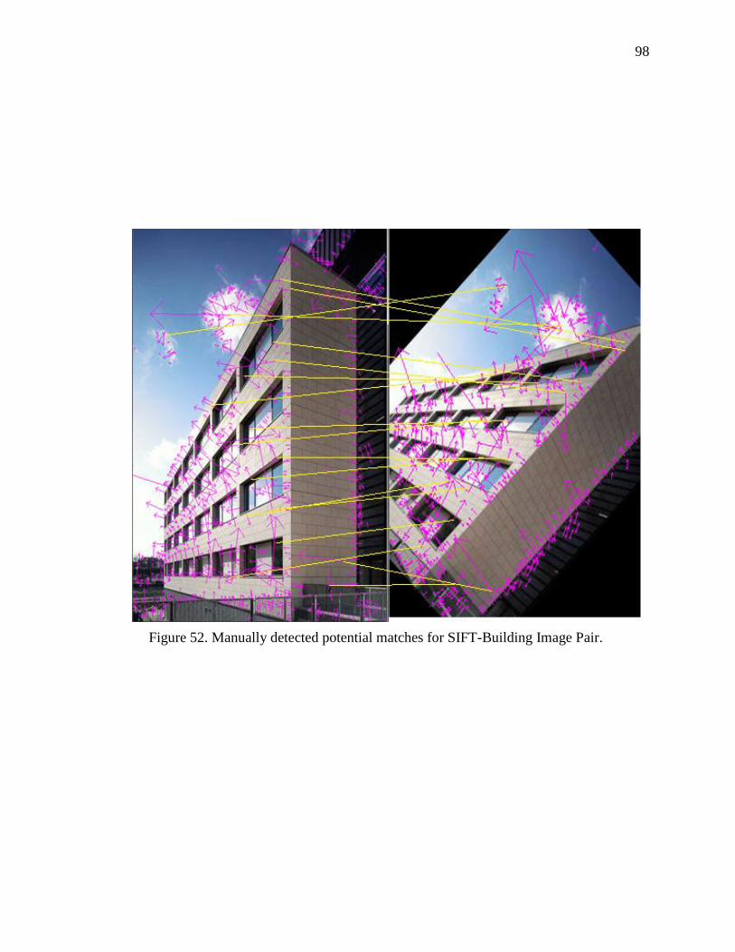
98
Figure 52. Manually detected potential matches for SIFT-Building Image Pair.

99
Figure 53. Manually detected potential matches for SURF-Window Image Pair.
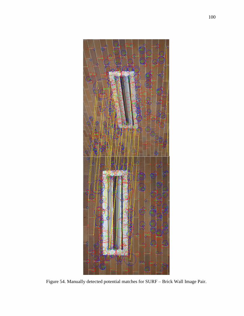
100
Figure 54. Manually detected potential matches for SURF – Brick Wall Image Pair.

101
Figure 55. Manually detected potential matches for SURF – Boat Image Pair.

102
Figure 56. Manually detected potential matches for SURF-Building Image Pair.

103
Figure 57. Manually detected potential matches for FAST-Window Image Pair.

104
Figure 58. Manually detected potential matches for FAST –Brick Wall Image Pair.

105
Figure 59. Manually detected potential matches for FAST-Boat Image Pair.
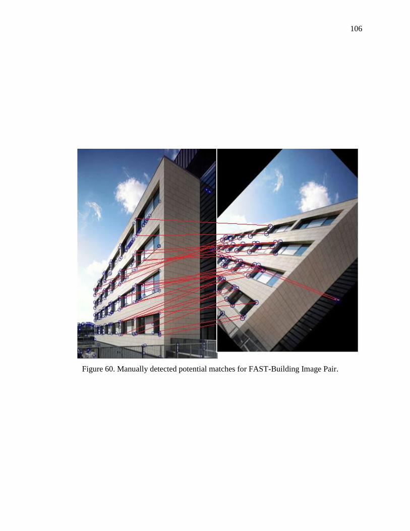
106
Figure 60. Manually detected potential matches for FAST-Building Image Pair.