a comparative study of site response in western washington
TRANSCRIPT

11
A Comparative Study of Site Response in Western Washington
Using Earthquake Data
by
Ruhollah Keshvardoost Jobaneh
A submitted to the Graduate Faculty of
Auburn University
in partial fulfillment of the
requirements for the Degree of
Master of Science
Auburn, Alabama
December 13, 2014
Keywords: Site response, amplification,
earthquake hazard, Seattle, Washington State
Copyright 2014 by Ruhollah Keshvardoost Jobaneh
Approved by
Lorraine W. Wolf, Chair, Professor of Geophysics
Ming-Kuo Lee, Professor of Geology
Ashraf Uddin, Professor of Geology

Abstract
Broadband and strong motion seismic data from three moderate to large
earthquakes were used to determine site response characteristics in the Seattle and
Tacoma, Washington, area. The three earthquakes chosen for analysis were the 2012 Mw
6.1 Vancouver Island earthquake, the 2012 Mw 7.8 Queen Charlotte Island earthquake,
and the 2014 6.6 Mw Vancouver Island earthquake. Resonant frequencies and relative
amplification of ground motions were determined using Fourier spectral rations of
velocity and acceleration records from three-component seismic stations within and
adjacent to the Seattle and Tacoma basins. Recordings from the sites were selected based
on their signal to noise ratios. Both the Standard Spectral Ratio (SSR) and the Horizontal-
to-Vertical Spectral Ratio (HVSR) methods were used in the analysis and results from
each were compared. Although 56% of the sites exhibited consistent results between the
two methods, other sites varied considerably. Sites that had acceptable recordings from
more than one of the earthquakes were compared. Using the results, several factors
postulated to influence site response were examined for this study. These included depth
to bedrock and age/type of geologic material. Although the scope of this study is limited,
results of the analysis suggest that sites located on the Pleistocene continental glacial drift
tend to have high amplification at 1-1.5 Hz by both HVSR and SSR results. Acceleration
data from the Seattle Liquefaction Array (SLA) were also used to determine the site
response in different depths. The spectra and the SSRs from this station indicate

consistent frequency characteristics of the near-surface amplification among the
earthquakes. The depth of the sediments to the bedrock along with the age and the type
of the geologic units are investigated as the two major factors involved in the SSR and
the HVSR results.

Dedication
This thesis is dedicated to my loving parents for their endless love, support, and
encouragement.

Acknowledgments
The author would like to thank Drs. Andy Frassetto, John Taber, and Chad
Trabant from IRIS for their help and support with acquiring and analysis of the data. My
appreciation is also extended to Dr. Charlotte Rowe from Los Alamos National
Laboratory (LANL) for her expertise, time, and guidance. Thanks to Drs. Thomas Pratt
and Arthur Frankel from Geological Society of America (GSA) for their contribution to
this research. I would also like to appreciate my committee member Dr. Ming-Kuo Lee
for his support, contribution and knowledge. My sincere appreciation goes to my advisor
and the head of my committee, Dr. Lorraine Wolf. This accomplishment would not be
possible without her dedication, patience, knowledge, intelligence, and support. I would
also like to thanks to my other committee member Dr. Ashraf Uddin for his help and
support both academically and spiritually. To all other Geology and Geography faculty,
staff and colleagues goes my gratitude for making this department such a wonderful place
to study and enjoy the life at the same time. My deepest gratitude goes to my parents for
their love, dedication, and support throughout this work.

Table of Contents
Abstract .......................................................................................................................... ii
Acknowledgments ........................................................................................................... v
List of Figures ...............................................................................................................vii
List of Tables................................................................................................................... x
List of Abbreviations ...................................................................................................... xi
Introduction ................................................................................................................... 1
Background and Geologic Setting .................................................................................. 4
Previous Work ............................................................................................................... 7
Analogues .................................................................................................................... 10
Methodology ............................................................................................................... 19
Results ......................................................................................................................... 29
Discussion ................................................................................................................... 80
Conclusion .................................................................................................................. 89
References ................................................................................................................... 91
Appendices .................................................................................................................. 96

List of Figures
Figure 1 Epicentral location of the earthquakes used in this study .................................................. 3
Figure 2 Stratigraphic column for the Puget Lowland.................................................................. 5
Figure 3 Map of observed and predicted amplification in 2009 Frankel’s study ................................. 9
Figure 4 Amplification ratio and corresponding shear-wave velocities for sites in Jammu city............. 11
Figure 5 HVSR curves in different part of Jammu city .............................................................. 12
Figure 6 Regions with the maximum amplification levels from HVSR in Ankara basin ..................... 14
Figure 7 Seismic zonation map for assessing the effects in the Ankara basin ................................... 15
Figure 8 Examples of observed and 1D modelled NHV curves in Vega Baja .................................. 16
Figure 9 Spectral ratios and H/V at La Lucia Ridge .................................................................. 18
Figure 10 Locations of the ten broadband stations selected for this study ....................................... 20
Figure 11 Strong motion stations on liquefaction map ............................................................... 22
Figure 12 Flowchart showing the analysis procedure ................................................................ 26
Figure 13 Example of a 3-component broadband seismogram used in this study .............................. 27
Figure 14 He component of acceleration from the liquefaction array ............................................. 28
Figure 15 The SSR results from the 2012 Queen Charlotte earthquake strong motion data ................. 30
Figure 16 The SSR results from the 2014 Vancouver Island earthquake strong motion data ............... 35
Figure 17 The SSR results from the 2012 Vancouver Island earthquake broadband data .................... 38
Figure 18 The HVSR results from the 2012 Queen Charlotte earthquake strong motion data .............. 41
Figure 19 The HVSR results from the 2014 Vancouver Island earthquake strong motion data ............ 47
Figure 20 The HVSR results from the 2012 Vancouver Island earthquake broadband data. ................ 51

Figure 21 Relative amplification in the 2012 Queen Charlotte earthquake (strong motion data) at 1 Hz
from HVSR and SSR analyses overlain on geology map .................................................. 57
Figure 22 Relative amplification in the 2012 Queen Charlotte earthquake (strong motion data) at 3 Hz
from HVSR and SSR analyses overlain on geology map .................................................. 58
Figure 23 Relative amplification in the 2012 Queen Charlotte earthquake (strong motion data) at 5 Hz
from HVSR and SSR analyses overlain on geology map .................................................. 59
Figure 24 Relative amplification in the 2012 Queen Charlotte earthquake (strong motion data) at 7 Hz
from HVSR and SSR analyses overlain on geology map .................................................. 60
Figure 25 Relative amplification in the 2012 Queen Charlotte earthquake (strong motion data) at 9 Hz
from HVSR and SSR analyses overlain on geology map .................................................. 62
Figure 26 Relative amplification in the 2012 Vancouver Island earthquake (broadband data) at 1 Hz from
HVSR and SSR analyses overlain on geology map ......................................................... 65
Figure 27 Relative amplification in the 2012 Vancouver Island earthquake (broadband data) at 3 Hz from
HVSR and SSR analyses overlain on geology map ......................................................... 66
Figure 28 Relative amplification in the 2012 Vancouver Island earthquake (broadband data) at 5 Hz from
HVSR and SSR analyses overlain on geology map ......................................................... 67
Figure 29 Relative amplification in the 2012 Vancouver Island earthquake (broadband data) at 7 Hz from
HVSR and SSR analyses overlain on geology map ......................................................... 68
Figure 30 Relative amplification in the 2012 Vancouver Island earthquake (broadband data) at 9 Hz from
HVSR and SSR analyses overlain on geology map ......................................................... 69
Figure 31 Relative amplification in the 2014 Vancouver Island earthquake (strong motion data) at 1 Hz
from HVSR and SSR analyses overlain on geology map .................................................. 72

Figure 32 Relative amplification in the 2014 Vancouver Island earthquake (strong motion data) at 3 Hz
from HVSR and SSR analyses overlain on geology map .................................................. 73
Figure 33 Relative amplification in the 2014 Vancouver Island earthquake (strong motion data) at 5 Hz
from HVSR and SSR analyses overlain on geology map .................................................. 74
Figure 34 Relative amplification in the 2014 Vancouver Island earthquake (strong motion data) at 7 Hz
from HVSR and SSR analyses overlain on geology map .................................................. 75
Figure 35 Relative amplification in the 2014 Vancouver Island earthquake (strong motion data) at 9 Hz
from HVSR and SSR analyses overlain on geology map .................................................. 76
Figure 36 Acceleration spectra against frequency at SLA station from the 2012 Queen Charlotte
earthquake ............................................................................................................ 78
Figure 37 Acceleration spectra against frequency at SLA station from the 2014 Vancouver Island
earthquake ............................................................................................................ 79
Figure 38 Horizontal depth slice showing P wave velocity in the depth of 2.5 km underlain by the station
locations ............................................................................................................... 84
Figure 39 SSR against frequency at SLA station referenced to GNW. ........................................... 86
Figure 40 SSR against frequency at SLA station referenced to the accelerometer located at the depth of
56.4m. ................................................................................................................. 87

List of Tables
Table 1 Broadband stations recorded the 2012 Vancouver Island earthquake .................................. 21
Table 2 Strong motion stations from the 2012 Queen Charlotte earthquake..................................... 23
Table 3 Strong motion stations from the 2014 Vancouver Island earthquake ................................... 24
Table 4 Earthquakes used in the analysis ................................................................................ 29
Table 5 The maximum values of SSR and HVSR from the 2012 Queen Charlotte earthquake at each
station in different frequencies ................................................................................... 55
Table 6 The maximum values of SSR and HVSR from the 2012 Vancouver Island earthquake at each
station in different frequencies ................................................................................... 63
Table 7 The maximum values of SSR and HVSR from the 2014 Vancouver Island earthquake at each
station in different frequencies ................................................................................... 70

List of Abbreviations
IRIS Incorporated Research Institution for Seismology
HVSR Horizontal to Vertical Spectral Ratio
SSR Standard Spectral Ratio
CSZ Cascadia Subduction Zone
GSA Geological Society of America

11
Introduction
The Cascadia Subduction Zone (CSZ) megathrust stretches from northern
Vancouver Island to California and separates the subducting Juan de Fuca plate from the
overriding North America plate (Fig. 1). This subduction zone produced the January 26,
1700, Cascadia earthquake, with an estimated moment magnitude of 8.7-9.2 (Atwater et
al., 2005). Several other significant earthquakes have occurred in the western part of
Washington in the past century. The April 13, 1949, 7.1 Mw Olympia earthquake, the
April 29, 1965, 6.7 Mw Olympia earthquake and the February 28, 2001, 6.8 Mw
Nisqually earthquake on which occurred very close to the epicenter of 1949 event, are
among the most important. Smaller magnitude earthquakes happen frequently (almost
once a month) (Barnett et al., 2009).
Situated above the CSZ, the Seattle and Tacoma metropolitan areas in the Puget
Lowland of western Washington are at risk from earthquake related damage. These
seismically active areas overlie sedimentary basins and are home to over 3.5 million
people. Since sedimentary basins affect seismic waves and often increase the level of
earthquake damage, it is crucial to gain a better understanding of earthquake waves as
they travel through basin sediments.
Site characteristics, such as fundamental period and wave amplification, are
influenced by sediment type, location, and thickness of sedimentary units, and can affect

ground shaking at a given location. Ground motions experienced at a site are a function
of the earthquake source, the wave path, and the characteristics (e.g., sediment type, local
geology, depth to bedrock) of the site itself. Much research by seismologists and
engineers has focused on understanding and predicting these site characteristics for
estimating seismic hazard in areas where the potential for large earthquakes exists. The
site effect can be represented by an empirical transfer function that captures the influence
of surficial geologic units on earthquake ground motions. Two common techniques used
in previous studies for approximating this transfer function are the horizontal-to-vertical
spectral ratios (HVSRs) and the standard spectral ratios (SSRs) (e.g., Frankel (1999,
2002, 2009), Molnar et al., (2004), Pratt (2006), Koçkar and Akgün (2012), Garcia-
Fernandez and Jimenez (2012)).
The goal of this study is to determine site effects on ground motions at several
locations near the urban centers of Seattle and Tacoma using broadband and strong
motion data acquired for three different earthquakes: (1) the October 28, 2012, Mw 7.8
Queen Charlotte earthquake (2) the April 24, 2014, Mw 6.6 Vancouver Island
earthquake, and (3) the November 8, 2012, Mw 6.1 Vancouver Island earthquake (Fig.
1). Results from this study will be compared with results from similar studies previously
conducted in this area. The SSR results will also be compared to the HVSRs to
investigate the consistency of the results at each method. This study will also explore the
two major factors affecting the ground motion amplification in the study area.

Fig. 1. Simplified tectonic map showing the epicentral locations of earthquakes used in this study. The Juan
de Fuca plate and the Explorer plate are subducting under the North America plate, forming the Cascadia
Subduction Zone. Stippled area indicates land.

Background and Geologic Setting
The main sources of earthquakes in the Pacific Northwest are associated with
plate motions involving the Pacific, North America, and Juan de Fuca plates (Fig. 1).
Strain accumulation resulting from these plate interactions is released through
earthquakes within the subducting Juan de Fuca plate, along the plate interface, or in the
overriding plate (Barnett et al., 2009). The Queen Charlotte fault, is an active transform
fault that forms a triple junction where it intersects the Explorer plate, the Juan de Fuca
plate and the North America plate, transitioning to become the CSZ.
The M 8.7 to 9.2 Cascadia earthquake in 1700 occurred along the CSZ and made
a fault rupture estimated to be approximately 1000 km long from northern California to
Vancouver Island in British Columbia with an average slip of 20 m (Atwater et al., 2005).
North-south shortening resulting from oblique plate convergence (Khazaradze et al.,
1999) has produced east-trending thrust faults and dextral strike-slip faults throughout the
Puget Lowland fore-arc basin. Crustal faulting in this area is the main mechanism for the
formation of several thick sedimentary basins (Brocher et al., 2001). Among these basins,
the Seattle and Tacoma basins pose the highest level of hazard because of their proximity
to large populations.

The stratigraphy of Seattle basin has been studied using surface exposures, industry
boreholes, and seismic profiles tied to the boreholes by many geoscientists (Fig. 2)
(Johnson et al., 1996; Brocher et al., 1998; Snelson et al., 2007; Troost and Booth, 2008).
Almost 1.1 km of
Fig. 2. Stratigraphic column for the Puget Lowland (Snelson et al., 2007).
unconsolidated Pleistocene and Holocene deposits at the top of the basin is assumed to be
the main cause of amplification of seismic waves (Frankel et al., 1999, 2002; Pratt et al.,

2003). The upper part of these deposits is a temporally and spatially complex collection
of glacial outwash till, lacustrine deposits, and recessional deposits that were formed
when the Puget Lowland was glaciated during at least six different episodes in the
Pleistocene (Booth, 1994). Well logs and seismic reflection data indicate that there are
sedimentary rocks of Eocene and Miocene age below these unconsolidated Holocene
deposits. The Miocene age Blakely Harbor Formation contains of siltstones,
conglomerates and non-marine sandstones (Fig. 2). The conglomerate clasts are poorly
sorted pebbles, cobbles, and boulders, of which about 85% are from Crescent Formation
(Johnson et al., 1994, 1996). The Eocene to Oligocene Blakely Formation consists of
different deep marine sequences. The Crescent Formation, which is stratigraphically
below the Blakely Formation, consists of basalt and minor interbeds of siltstone, tuff, and
conglomerate (Johnson et al., 1994; Jones 1996; Snelson et al., 2007).
Previous Work
Many studies have used ground motions to characterize the effects of sedimentary
basins on seismic waves. Examples include Frankel (1999, 2002, and 2009), Molnar et al.
(2004), Pratt et al. (2006), Ghasemi et al. (2009), and Koçkar and Akgün (2012).
Frankel (1999) analyzed seismograms from 21 earthquakes (ML 2.0-4.9) recorded
by digital seismographs situated on wide variety of geologic units and developed a new
inversion procedure to estimate site response. He observed high amplifications on
artificial fill, more moderate amplification for sites on stiff Pleistocene soils, and low
response for rock sites. The results of his study also showed a strong 2-Hz resonance at
sites with surficial layers of fill and younger alluvium.
In another study, Frankel et al. (2002) used the recordings of the M 6.8 Nisqually
earthquake and its ML 3.4 aftershock to study site response and basin effects for 35
locations in Seattle, Washington. This study used SSRs, or Fourier spectral ratios of
horizontal ground motions recorded at soft sediment sites relative to a reference site. He
observed that sites on artificial fill and young alluvium had the largest 1-Hz amplification
for both the mainshock and aftershock.

Molnar et al. (2004) examined site responses in Victoria, British Columbia, using
weak ground motion recordings of the 2001 Nisqually earthquake in Washington. They
analyzed the data using both the SSR method and the HVSR method and observed a
considerable variation in acceleration spectra across the city due to local site conditions.
The HVSR method uses the average of the horizontal components of the shear wave
divided it by the vertical component. For their reference recordings for the SSR
calculations, they used stations at thin soil sites (< 3 m) having a flat-amplitude spectra at
frequencies less than 10 Hz. They found that sites with thicker soils (5-10 m) showed
peak amplitudes at 2-5 Hz.
Pratt et al. (2006) used SSR and HVSR methods at 47 sites in the Puget
Lowland and observed significant amplification of 1.5- to 2.0-Hz shear waves
within sedimentary basins. The SSR curves at thick basin sites showed peak
amplification at frequencies of 3 to 6 Hz and lower amplification at frequencies
above 6 Hz. They proposed that the attenuation within the basin strata is the main
cause of the spectral decay at frequencies above the amplification peak.
Frankel (2009) studied the effect of basins on site response in the Puget
Lowland using 3D finite-difference simulations for five earthquakes, including
the M 6.8 Nisqually earthquake. His modeling suggests a dependence of
amplification on the directivity of the earthquake rupture. Earthquake directivity
is the focusing of wave energy along a fault in the direction of rupture. He found
that S waves are focused toward the southern margin of the Seattle basin in an
area \that experienced increased chimney damage from the Nisqually earthquake.
Chimney damage is used as a proxy for the intensity of ground shaking (Fig. 3).

Fig. 3. Maps indicate observed (green circles) and
predicted (black circles) amplification at 1 Hz for four
earthquakes plotted on map of surface geology. Circle
size is proportional to 1 Hz amplification. Arrows show
direction of seismic wave propagation based on the location of the earthquake. Stations with no
green circles did not record that particular earthquake (Frankel, 2009).

Analogues
In this section, four investigations from India, Turkey, Spain and South Africa
using methods similar to those in this study are presented and serve as analogues to
validate the modeling approach.
Jammu City, India
Passive seismic methods including HVSR and microtremors were used to
investigate the site response at 30 station locations located in frontal part of the Himalaya
Mountains, which contain soft sediments that have strong effects on recorded ground
motions (Mahajan et al., 2012). Mahajan et al. (2012) used shear-wave velocities from
the top 30 m l of Pleistocene and Holocene sediments overlying Lower Miocene bedrock,
along with seismic data from the 20 October, 1991 (Mb 6.8) Chamilo earthquake to
calculate the site response spectrum at the sites. Buildings of different heights have
different resonant frequencies, making amplification in certain period ranges an
important engineering concern. The response spectrum of the sites indicates a five to
seven times increase in peak ground acceleration for single or two-story buildings. Fig. 4
shows amplification ratios, periods, and shear wave velocities at different sites in the N-S
and NW-SE directions (Mahajan et al., 2012). The study show eight to twelve times
increase in amplification at 2 to 3 Hz frequency in the central part and 1.75 to 2 Hz in
peripheral parts of the city.

Fig. 4. Amplification ratios and corresponding shear-wave velocities for sites in Jammu city. Upper panel
(a) shows results from N-S profile; lower panel (b) shows results from NW-SE profile. (From Mahajan et
al., 2012).
The stations located in the central part of the city (e.g., Sites 14 and 9) show HVSR
curves with clear peaks in comparison to the sites in the northwestern and southwestern

part of the town (e.g., Sites 7, 25) (Fig. 5). Broad HVSR peaks imply a low impedance
contrast between basement and overlying sediments and only provide a range of
amplification values. Overall, it can be concluded that HVSR can only be successful in
areas with high impedance contrast (Mahajan et al., 2012).
Fig. 5. HVSR curves in different part of Jammu city. Sharp peaks are associated with high impedance
contrast as opposed to broad peaks that are indicative of low impedance contrast from Mahajan et al.,
(2012).
Ankara, Turkey

Koçkar and Akgün (2012) collected 352 microtremor measurements in the
western part of the Ankara basin within the Plio-Pleistocene fluvial and Pleistocene and
Holocene alluvial and terrace sediments. They used HVSRs of these measurements to
calculate the fundamental periods and amplification of their sites. These measurements
were correlated with the in situ measurements of dynamic properties of geologic
information. The results from this study indicate that three main factors were involved in
the site response: (1) age of the geologic formation, (2) depth of the sediments to the
bedrock, and (3) non-uniform subsurface configuration. Due to the presence of low-
velocity deposits near the surface, stations located at Pleistocene and Holocene sediments
show high amplification at longer periods than the older Plio-Pleistocene fluvial
sediments. The HVSR results further showed that the variation of the fundamental period
agreed well with maximum amount of amplification at a given site. Pleistocene and
Holocene sediments, which are the thicker and unconsolidated, possess low shear wave
velocity and show higher amplification results at fundamental periods.
Using the HVSR results, the results of Vs30 measurements (average shear wave
velocity in the upper 30 m), and geologic information, Koçkar and Akgün (2012) created
a site class zonation map for the Ankara basin. The map provides a tool to assess and
mitigate the potential risk from future seismic events in the study area (Fig.7).

Fig
. 6.
Map
of
the
regio
ns
wit
h t
he
max
imum
am
pli
fica
tion
lev
els
from
HV
SR
met
hod i
n A
nkar
a bas
in (
Koçk
ar a
nd A
kgün
,
2012
).

Fig. 7. Seismic zonation map for assessing the effects in the Ankara basin. The plot includes the site
classification map based on average Vs30 measurements and the maps of HVSR regarding resonance
periods and maximum amplifications (Koçkar and Akgün, 2012).
Vega Baja, Spain
Garcia-Fernandez and Jimenez (2012) conducted ambient noise surveys at 90
sites over the central part of the Lower Segura River basin in the Vega Baja region,
located southeast of the Iberian Peninsula. This dataset, along with geological,
geotechnical, and other geophysical data, was used to identify multiple peaks in some of
the HVSR curves. The dataset represents different impedance contrasts at depths that
were modeled to characterize the Vega Baja soils units, depth to the bedrock, and depth
to the rock units. The depth to the bedrock varies in different parts of the basin from 30 m
to 50 m. The average of the shear-wave velocity over the soil unit is approximately 200
m/s, and the average velocity in the top 30 m is around 300 m/s.

In Fig. 8, three examples of experimental and 1D synthetic H/V curves from their
paper are shown together with three generalized models indicating the subsurface
structure in Vega Baja. Model 1 sites are mainly located at the central and western part of
the Lower Sengura basin and the northern border of the Hurchillo, Benejuzar and
Guardamar Mountains. Model 2 sites are in the Orihuela-Callosa Ranges. Model 3 sites
are located in the north, south, and east sections of the Lower Segura basin. The results of
the study show a strong relationship of fundamental periods with lithological variation
with sediment thickness (Garcia-Fernandez and Jimenez, 2012).
Fig. 8. (a) Examples of observed (light gray line =mean value) and 1D modeled H/V (dark gray line)
values; (b) generalized 1D soil models in Vega Baja (Garcia-Fernandez and Jimenez, 2012).

Durban, South Africa
A refined version of the HVSR generated by cultural seismic noise has been used
to study the seismic response of several sites in Durban area of South Africa (Fernandez
and Brandt, 2000). Three components of two ambient noise samples separated by several
minutes were acquired at 18 sites. Although the data samples were different in time and
frequency content, the HVSR curves look very similar in most of the pairs (Fig. 9). Not
only were the frequency peaks almost identical, but also the ranges of amplifications
were very similar. The method used in this study is based on using a hard-rock site (“the
Kloof”) as a reference and comparing all the soft sites relative to the hard-rock site (Fig.
9). This comparison with a hard- rock site helps to gain a better understanding of the
physical meaning of the site response. Results from this study showed that the influence
of the layer system on the vertical component of motion does not exceed the value of
two; therefore, it can be assumed that the majority of amplification is due to the
horizontal motion.
Fig. 9 shows the HVSRs at two different times at two of the sites that are
underlain with unconsolidated sediments. Fig. 9 also includes the site response at each
site relative to the hard rock site, which is thought to be in direct relation to the
amplification factor.

Fig. 9. Left column: two HVSRs (a and b) at La Lucia Ridge (consolidated sand). Site response (c) is with
respect to hard rock site “The Kloof.” Right column: two HVSRs (a and b) at Warner beach (sand). Site
response (c) is again with respect to hard rock site “The Kloof” (Fernandez and Brandt, 2000).
a
b
c
b
c
a

Methodology
This section provides information about data acquisition and analysis. Data
acquisition includes station selection and sources for broadband, strong motion, and other
supporting data. Data analysis includes the methods used to process all the acquired
seismic data. Three-component broadband data record velocity and cover a wide
frequency band (0.01 to 25 Hz). Strong motion data measure acceleration and are useful
for recording large-amplitude, high frequency (0 to 100 Hz) seismic waves.
Data Acquisition
Broadband data
Seismic stations used in this study are located in western Washington, most of
which are within Seattle and Tacoma basins (Fig. 10). Most of the sites are underlain by
thick sedimentary sequences that fill the basins; however, in a few cases the bedrock is
exposed or located very close to the surface. Three-component data from 16 broadband
stations of the University of Washington (UW) and Transportable Array (TA) networks
were selected and the data were downloaded from the Incorporated Research Institutions
for Seismology (IRIS) data center (http://service.iris.edu/irisws/timeseries/docs/1/builder)
for the November 8th, 2012 Vancouver Island earthquake. All data have a 40-Hz
sampling frequency with the length of 40 minutes. Ten stations having acceptable signal

to noise ratio (more than 2) were selected and cover areas with different liquefaction
susceptibility (Fig. 10). The station name, network, latitude, longitude, and elevation of
each station are shown in Table 1.
Fig. 10. Locations of ten broadband stations selected for this study overlain on liquefaction susceptibility
map (Palmer et al., 2004).

Table 1. Broadband stations recorded the 2012 Vancouver Island earthquake.
Network Station Latitude Longitude Elevation(m) Geologic Unit
TA B05D 48.2641 -122.096 153 Pleistocene continental glacial drift
TA D03D 47.5347 -123.089 262 Pleistocene continental glacial drift
UW DOSE 47.7172 -122.972 53 Pleistocene continental glacial drift
UW GNW 47.56413 -122.825 220 Paleogene and Neogene intrusive rock
UW LON 46.7506 -121.81 853 Paleogene and Neogene fragmental volcanic rock
UW LRIV 48.0575 -123.504 293 Pleistocene continental glacial drift
UW RATT 47.42546 -121.803 440 Paleogene and Neogene fragmental volcanic rock
UW SP2 47.55629 -122.249 30 Pleistocene continental glacial drift
UW TOLT 47.69 -121.69 541 Paleogene and Neogene volcanic rock
UW WISH 47.11698 -123.771 45 Pleistocene and Holocene alluvium
Strong motion data
Forty-seven three-component acceleration records were acquired from strong
motion stations for the Mw 7.8 Queen Charlotte Island earthquake and Mw 6.6
Vancouver Island earthquake that occurred at 3:04:08 am on October 28th, 2012, and
3:10:12 am on April 24th, 2014, respectively. The IRIS URL Builder was used to
download 40 minutes of data with 100-Hz sampling frequency (Fig. 11). Tables 2 and 3
list the station name, location, elevation, and geologic unit of each station used in the
study.

Fig. 11. Strong motion stations overlain on liquefaction map (Palmer et al., 2004).

Table 2. Strong motion stations for the 2012 Queen Charlotte earthquake.
Network Station Latitude Longitude Elevation
(m)
Geologic Unit
UW ALCT 47.65 -122.04 55 Pleistocene continental glacial drift
UW ALKI 47.58 -122.42 1 Pleistocene and Holocene alluvium
UW BABE 47.61 -122.54 83 Pleistocene continental glacial drift
UW DOSE 47.72 -122.97 53 Pleistocene continental glacial drift
UW EARN 47.74 -122.04 159 Pleistocene continental glacial drift
UW ERW 48.45 -122.63 389 Pleistocene continental glacial drift
UW EVCC 48.01 -122.2 0 Pleistocene continental glacial drift
UW EVGW 47.85 -122.15 10 Pleistocene continental glacial drift
UW FINN 47.72 -122.23 121 Pleistocene continental glacial drift
UW HICC 47.39 -122.3 115 Pleistocene continental glacial drift
UW LON 46.75 -121.81 853 Paleogene and Neogene fragmental volcanic rock
UW LRIV 48.06 -123.5 293.8 Pleistocene continental glacial drift
UW LYNC 47.83 -122.29 19 Pleistocene continental glacial drift
UW MARY 47.66 -122.12 11 Pleistocene and Holocene alluvium
UW MEAN 47.62 -122.31 37 Pleistocene continental glacial drift
UW MNWA 47.57 -122.53 8 Paleocene to Miocene marine
sedimentary rock
UW NIHS 47.74 -122.22 137 Pleistocene continental glacial drift
UW NOWS 47.69 -122.25 21 Pleistocene and Holocene alluvium
UW PAYL 47.19 -122.31 10 Pleistocene and Holocene alluvium
UW PNLK 47.58 -122.03 128 Pleistocene continental glacial drift
UW RATT 47.43 -121.8 440 Paleogene and Neogene fragmental
volcanic rock UW SP2 47.56 -122.25 30 Pleistocene continental glacial drift
UW SQM 48.07 -123.05 45 Pleistocene continental glacial drift
UW SVOH 48.29 -122.63 22 Pleistocene continental glacial drift
UW SWID 48.01 -122.41 62 Pleistocene continental glacial drift
UW TOLT 47.69 -121.69 541 Paleogene and Neogene volcanic rock
UW WISH 47.12 -123.77 45 Pleistocene and Holocene alluvium

Table 3. Strong motion stations for the 2014 Vancouver Island earthquake.
Network Station Latitude Longitude Elevation
(m)
Geologic Unit
UW ALCT 47.65 -122.04 55 Pleistocene continental glacial drift
UW ALKI 47.58 -122.42 1 Pleistocene and Holocene alluvium
UW BABE 47.61 -122.54 83 Pleistocene continental glacial drift
UW DOSE 47.72 -122.97 53 Pleistocene continental glacial drift
UW EARN 47.74 -122.04 159 Pleistocene continental glacial drift
UW ERW 48.45 -122.63 389 Pleistocene continental glacial drift
UW EVCC 48.01 -122.2 0 Pleistocene continental glacial drift
UW EVGW 47.85 -122.15 10 Pleistocene continental glacial drift
UW FINN 47.72 -122.23 121 Pleistocene continental glacial drift
UW HICC 47.39 -122.3 115 Pleistocene continental glacial drift
UW LON 46.75 -121.81 853 Paleogene and Neogene fragmental
volcanic rock
UW LRIV 48.06 -123.5 293.8 Pleistocene continental glacial drift
UW LYNC 47.83 -122.29 19 Pleistocene continental glacial drift
UW MARY 47.66 -122.12 11 Pleistocene and Holocene alluvium
UW MEAN 47.62 -122.31 37 Pleistocene continental glacial drift
UW MNWA 47.57 -122.53 8 Paleocene to Miocene marine sedimentary rock
UW NIHS 47.74 -122.22 137 Pleistocene continental glacial drift
UW NOWS 47.69 -122.25 21 Pleistocene and Holocene alluvium
Data Analysis
There are three main factors affecting the recorded waveform of a seismic signal:
the source, the path, and the site. To isolate the site response from the other two factors,
we use seismic recordings from the same earthquake at stations that are approximately on
the same azimuth. This eliminates the effect of the source and partially reduces the
influence of path. The distances between the stations are relatively close in comparison to
the source-receiver distance; however, seismic waves experience attenuation as a

function of distance and this effect is accounted for in the data processing by using an
attenuation correction (discussed below).
Three-component Broadband data
After downloading the broadband data, a bandpass filter (0.2-15Hz) (Langston,
[http://www.ceri.memphis.edu/people/clangstn/, accessed on 28/7/2014]) was applied to
each component. A segment of data with a length of 75 seconds (3001 samples) starting
before the S-wave was extracted from each waveform for each station. Then the data
were demeaned, detrended, and tapered, before calculating the power spectra for each
component (horizontal east (He), horizontal north (Hn), and vertical (Vz) (Fig. 12).
MATLABTM’s power spectral density function (PSD) was used for this purpose. The
spectral amplitudes were corrected for attenuation and spherical spreading using the
following equation:
Ac (f) = Ao (f) r0.5 e πft/Qs(f) (1)
where Ao (f) is observed amplitude, Ac (f) is corrected amplitude, f is frequency, t is
travel time, r is source-receiver distance, and Qs (f) is a frequency-dependent s-wave
attenuation factor (Pratt and Brocher, 2006). The bedrock relation of Qs (f) = 380 f 0.39
(Atkinson, 1995) was utilized in the equation to correct for attenuation and spherical
spreading. The source-receiver distance was estimated using the geographic coordinates
of the epicenter and stations. Due to the shallow depth (<15 km) of the focal point in all
the events used in this study, the source-receiver distance approximately equals the arc
distance used in the correction. According to Atkinson (1995), the value of r0.5 is

preferred to r for source-receiver distances of more than 230 km. To calculate the travel
time, the p-wave arrival was subtracted from the exact time of the earthquake.
To calculate the HVSR, the spectra from the horizontal components (Hn and He)
were averaged and divided by the vertical component (Vz). The results were smoothed
using a MATLABTM function that uses a 20-point moving average. The data processing
procedure is shown schematically in Fig. 12.
Fig. 12. Flowchart showing data processing steps for data used in this study.
Load data
Apply bandpass filter
Demean and Detrend
Taper
Extract segment starting before
the S-wave
Calculate
spectra (PSD
function)
Smooth
Calculate HVSR and SSR
Apply attenuation correction

Strong motion data
The processing of strong motion data was similar to that used for the broadband data.
However, the bandpass filter used low- and high-end frequencies of 0.2 and 25 Hz,
respectively, and the segments were 70 s (7001 samples) long (Fig. 13). A smoothing
function was applied to the strong motion data using a 5-point span window.
Fig. 13. Example of a 3-component broadband seismogram used in this study. The extracted data segment
(red rectangle) begins shortly before the S wave and continues for 70 seconds.
Liquefaction array
One strong motion station, SLA, (also known as Seattle liquefaction array)
recorded acceleration data from several depths (0 m (surface), 4.5 m, 44.9 m, and 56.4
Sample number
Vel
oci
ty

m). The site has a high level of noise introduced by trains traveling nearby. To eliminate
the train noise, a bandpass filter with the cut off frequencies of 0.02 and 25 Hz was used
on each component before extracting the segment and calculating the SSRs (Fig. 14).
Fig. 14. Example of effect of bandpass filter on He component of acceleration from the liquefaction array
before (upper plot) and after (lower plot) its application. High-amplitude noise (seen between 3.8 x 10 -5
and 4.0 x 10⁻⁵ on upper plot) is reduced significantly after filtering (lower plot).
Acc
eler
atio
n
Samples

Results
This chapter includes the HVSR and SSR results from the 2012 Queen Charlotte
strong motion data, the 2014 Vancouver Island strong motion data, and the 2012
Vancouver Island broadband data. It also contains the results from the Seattle
liquefaction array. Details for each earthquake are included in Table 4.
Table 4. Earthquakes used in the analysis.
Event number 1 2 3
Location Queen Charlotte Vancouver Island Vancouver Island
Date 10/28/2012 4/24/2014 11/8/2012
Time 03:04:08 UTC 03:10:12 UTC 02:01:50 UTC
Latitude 52.788° N 49.8459° N 49.231° N
Longitude 132.101° W 127.444° W 128.477° W
Magnitude MW7.8 MWW6.6 MW6.1
Depth 14.0 km 11.4 km 13.7 km
Data type Strong motion Strong motion Broadband
Sampling rate 100 samples/sec 100 samples/sec 40 samples/sec
SSR Results
1. The 2012 Queen Charlotte Earthquake
Fig. 15 shows the SSR plots from the 2012 Queen Charlotte earthquake strong
motion data organized by the local geologic environment of the station location. Out of
the 16 stations located on Pleistocene continental glacial drift, 11 show a peak at ~1 Hz

frequency. In contrast, fundamental peak frequencies at 3 Hz are observed at DOSE and
SP2 stations. Most of the stations indicate low amplification at frequencies higher than 6
Hz. Secondary peaks are also observed at 2 Hz at LRIV, LYNC, EVCC, and NIHS.
(a) Pleistocene continental glacial drift
Frequency Frequency
SS
R
SS
R
SS
R
0.1 10
200

Pleistocene continental glacial drift (continued)
Frequency Frequency
SS
R
SS
R
SS
R

(b) Paleogene and Neogene volcanic rock
Frequency Frequency
Frequency
SS
R
SS
R
SS
R
0.1 10
200
10 0.1
200

(c) Pleistocene and Holocene alluvium
Frequency Frequency
Frequency
SS
R
SS
R
SS
R
10 0.1
10
200

(d) Paleogene and Neogene fragmental volcanic rock and Paleocene to
Miocene marine sedimentary rock
Fig. 15. SSR results from the 2012 Queen Charlotte earthquake strong motion data. Results are
displayed with respect to underlying geology, as determined from Washington Department of Natural
Resources (http://www.dnr.wa.gov/BusinessPermits/Pages/PubMaps.aspx) last accessed on 8/8/2014.
(a) Pleistocene continental glacial drift, (b) Paleogene and Neogene volcanic rock, (c) Pleistocene and
Holocene alluvium, (d) Paleogene and Neogene fragmental volcanic rock and Paleocene to Miocene
marine sedimentary rock. Refer to Fig. 12 and Table 2 for station locations. The insets show the full
extent of the some larger peaks.
TOLT, which is the only station located on Paleogene and Neogene volcanic rock,
shows peaks at 2 and 3 Hz. Three out of five stations located on Pleistocene and
Holocene alluvium have peaks at 1 and 3 Hz, with the exception of ALKI (0.4 Hz) and
MARY (2 Hz). Contrary to other stations located in this type of geology, WISH indicates
a flat response at all frequencies. LON and MNWA, located on Paleogene and Neogene
fragmental volcanic rock and Paleocene to Miocene marine sedimentary rock,
respectively, also show a flat response at all frequencies.
2. The 2014 Vancouver Island earthquake
Frequency Frequency
SS
R

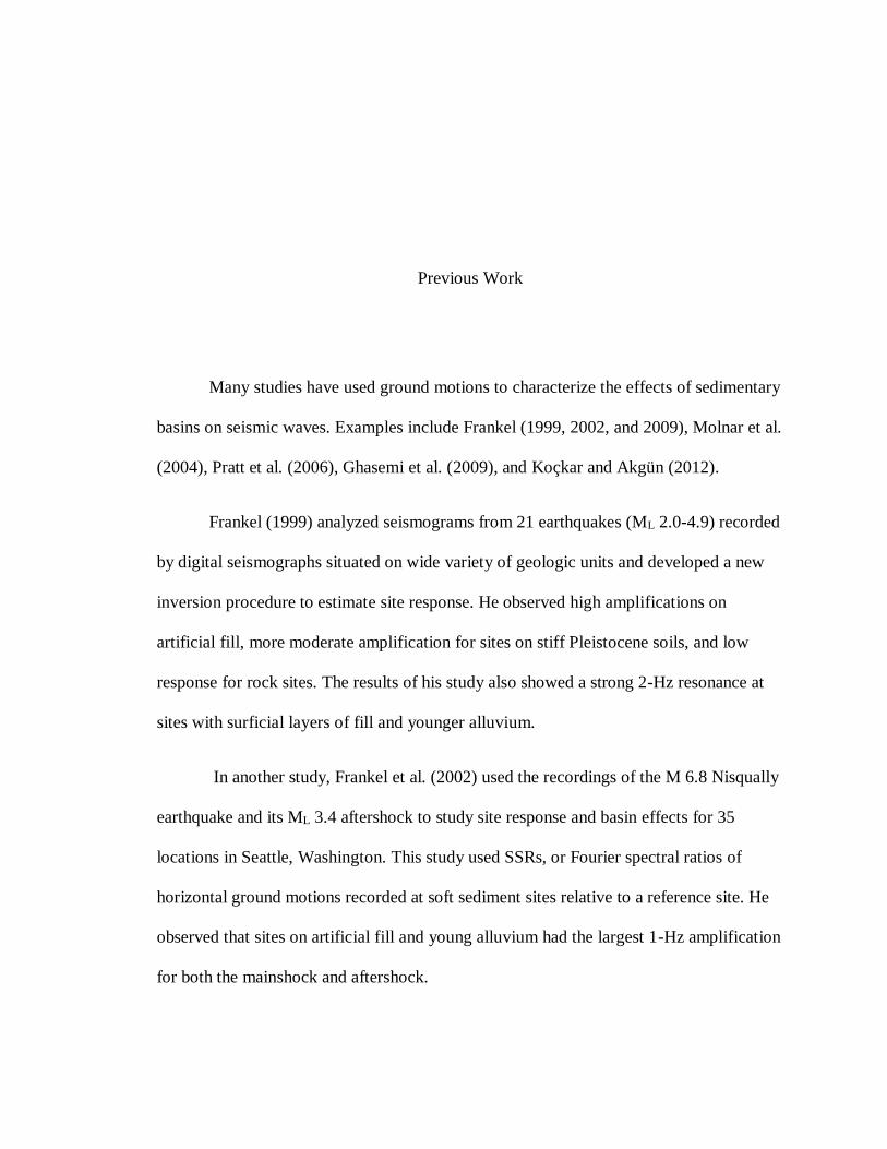
Fig. 16 shows the SSR plots for strong motion data from the 2014 Vancouver Island
earthquake organized by the local geologic environment of the station location.
(a) Pleistocene continental glacial drift
Frequency Frequency
SS
R
SS
R
SS
R
10 0.1
300
10 0.1
300

Pleistocene continental glacial drift (continued)
Frequency
Frequency Frequency
SS
R
SS
R
SS
R
(b) Paleogene and Neogene volcanic rock
(c) Pleistocene and Holocene alluvium
Fig. 16. The SSR results from the 2014 Vancouver Island earthquake strong motion data. Results are
displayed with respect to underlying geology, as determined from Washington Department of Natural
Resources (http://www.dnr.wa.gov/BusinessPermits/Pages/PubMaps.aspx) last accessed on 8/8/2014.
(a) Pleistocene continental glacial drift, (b) Paleogene and Neogene volcanic rock, (c) Pleistocene and
Holocene alluvium. Refer to Fig. 12 and Table 3 for station locations. The insets show the full extent
of larger peaks. The station PNLK is plotted on a different scale.
Frequency
Frequency Frequency
SS
R
SS
R
SS
R
10 0.1
300

For the 2014 Vancouver Island earthquake, peaks from 0.6 to 8 Hz are observed
on stations located on Pleistocene continental glacial drift. Five stations out of 11 share a
peak at 1 to 1.5 Hz. However, there is little consistency in the peak frequencies in terms
of the site geology. DOSE shows large peaks at 3 and 5 Hz. CDMR, KINR, and ELW
indicate peaks at 7 Hz. ALCT, BEVT, and EVGW have peaks at 0.7 to 0.8 Hz.
The response from TOLT (peaks at 1.5, 3, 5.5, and 7 Hz), which is located on
Paleogene and Neogene volcanic rock, is quite similar to its response from the 2012
Queen Charlotte earthquake. Likewise, the responses from all stations located in
Pleistocene and Holocene alluvium are similar to those from 2012 Queen Charlotte
earthquake located in the same type of geology. Despite differences on SSR relative
amplification values, peak frequencies at 11 stations are the same as those observed from
the 2012 Queen Charlotte Island earthquake.
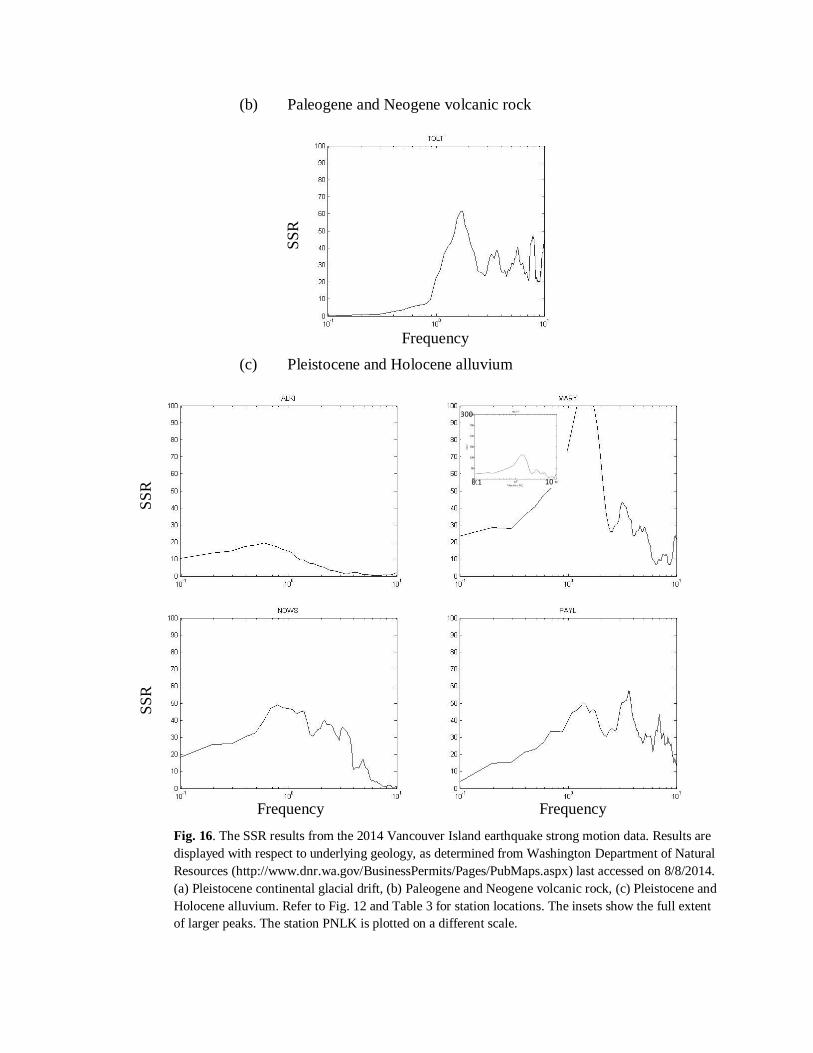
3. The 2012 Vancouver Island earthquake
Fig. 17 shows the SSR plots from broadband data from the 2012 Vancouver
Island earthquake organized by site geology at the station location.
(a) Pleistocene continental glacial drift
Frequency Frequency
SS
R

(b) Paleogene and Neogene volcanic rock
Frequency Frequency
Frequency
Frequency
SS
R
SS
R
SS
R
10 0.1
200
(c) Pleistocene and Holocene alluvium
(d) Paleogene and Neogene fragmental volcanic rock
Fig. 17. SSR results from the 2012 Vancouver Island earthquake broadband data. Results are displayed
with respect to underlying geology, as determined from Washington Department of Natural Resources
(http://www.dnr.wa.gov/BusinessPermits/Pages/PubMaps.aspx) last accessed on 8/8/2014. (a) Pleistocene
continental glacial drift, (b) Paleogene and Neogene volcanic rock, (c) Pleistocene and Holocene alluvium,
(d) Paleogene and Neogene fragmental volcanic rock. Refer to Fig. 11 and Table 1 for station locations.
Insets show the extent of the larger peaks
The SSR results from 2012 Vancouver Island earthquake broadband data show
consistent results for stations located on the Pleistocene continental glacial drift. All of
these stations show peaks at 3 Hz and a flat response at lower frequencies. TOTL show
peaks at 3, 5, and 7 Hz, which is quite similar to the response from this station in the
Frequency
Frequency Frequency
SS
R
SS
R

previous earthquakes. The only station located on the Pleistocene and Holocene alluvium,
WISH, shows a peak at 8 Hz. Stations located on Paleogene and Neogene fragmental
volcanic rock, LON and RATT, show a relatively flat response, except for the
frequencies higher than 7 Hz at station RATT.
HVSR Results
1. The 2012 Queen Charlotte earthquake
Fig. 18 shows the HVSR plots from strong motion data for the 2012 Queen
Charlotte organized by site geology at the station location.
(a) Pleistocene continental glacial drift
Frequency Frequency
HV
SR
H
VS
R
10 0.1
20

Pleistocene continental glacial drift (continued)
Frequency Frequency
HV
SR
H
VS
R
HV
SR

Pleistocene continental glacial drift (continued)
Frequency Frequency
HV
SR
H
VS
R
HV
SR

(a) Paleogene and Neogene volcanic rock
(b) Pleistocene and Holocene alluvium
Frequency
Frequency Frequency
HV
SR
H
VS
R
HV
SR
10 0.1
20
(c) Paleogene and Neogene fragmental volcanic rock
(d) Paleocene to Miocene marine sedimentary rock
Frequency
HV
SR
HV
SR
HV
SR
Frequency Frequency
Frequency
10 0.1
20

(e) Paleogene and Neogene intrusive rock
Fig. 18. HVSR results from the 2012 Queen Charlotte earthquake strong motion data. Results are
displayed with respect to underlying geology, as determined from Washington Department of Natural
Resources (http://www.dnr.wa.gov/BusinessPermits/Pages/PubMaps.aspx) last accessed on 8/8/2014.
(a) Pleistocene continental glacial drift, (b) Paleogene and Neogene volcanic rock, (c) Pleistocene and
Holocene alluvium, (d) Paleogene and Neogene fragmental volcanic rock, (e) Paleocene to Miocene
marine sedimentary rock, (f) Paleogene and Neogene intrusive rock. Refer to Fig. 12 and Table 2 for
station locations.
Four out of five stations located on Pleistocene and Holocene alluvium show
different HVSR peaks in comparison to the SSR results for the same earthquake, except
for PAYL, which shows the same peaks at 1 and 3 Hz. The peak frequencies include 1,
1.5, 2, 3, 3.5, 5, and 6 Hz. Large peaks at 3.5 and 6 Hz are observed on the WISH HVSR
plot, which is different with its flat response on SSR plot. LON and MNWA, which are
located on Paleogene and Neogene fragmental volcanic rocks and Paleocene to Miocene
marine sedimentary rock, respectively, show the same peak frequencies as seen on the
SSR plots.
2. The 2014 Vancouver Island earthquake
Frequency
HV
SR

Fig. 19 shows the HVSR plots from strong motion data from the 2014 Vancouver
Island earthquake organized by site geology at the station location.
(a) Pleistocene continental glacial drift
Frequency Frequency
HV
SR
H
VS
R
HV
SR
10 0.1
20

Pleistocene continental glacial drift (continued)
(b) Paleogene and Neogene volcanic rock
Frequency Frequency
Frequency
HV
SR
HV
SR
H
VS
R
10 0.1
20

(c) Pleistocene and Holocene alluvium
Frequency Frequency
HV
SR
H
VS
R
10 0.1
20

(d) Paleogene and Neogene intrusive rock
Fig. 19. HVSR results from the 2014 Vancouver Island earthquake strong motion data. Results are
displayed with respect to underlying geology, as determined from Washington Department of Natural
Resources (http://www.dnr.wa.gov/BusinessPermits/Pages/PubMaps.aspx) last accessed on 8/8/2014.
(a) Pleistocene continental glacial drift, (b) Paleogene and Neogene volcanic rock, (c) Pleistocene and
Holocene alluvium, (d) Paleogene and Neogene intrusive rock. Refer to Fig. 12 and Table 3 for
station locations. The insets show the extent of larger.
Peaks at 7 Hz are observed at stations ALCT, BEVT, ELW, FINN, LYNC, and
KINR. Other stations have peaks at 1, 2, 4, 5, and 9 Hz. TOLT shows consistent peaks
relative to the previous event (2012 Queen Charlotte earthquake) with peaks at 1, 5, and 7
Hz.
Stations located on Pleistocene and Holocene alluvium show rather different
results compared to the SSRs. Three of the stations share peaks at 2 to 3 Hz; two of them
repeat the peak at 6 Hz.
Frequency
HV
SR
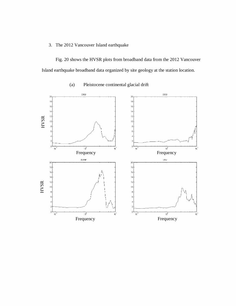
3. The 2012 Vancouver Island earthquake
Fig. 20 shows the HVSR plots from broadband data from the 2012 Vancouver
Island earthquake broadband data organized by site geology at the station location.
(a) Pleistocene continental glacial drift
Frequency Frequency
Frequency Frequency
HV
SR
H
VS
R

(b) Paleogene and Neogene volcanic rock
(c) Pleistocene and Holocene alluvium
Frequency
HV
SR
H
VS
R
HV
SR
Frequency
Frequency
10
80
0.1

(d) Paleogene and Neogene intrusive rock
(e) Paleogene and Neogene fragmental volcanic rock
Fig. 20. HVSR results from the 2012 Vancouver Island earthquake broadband data. Results are
displayed with respect to underlying geology, as determined from Washington Department of Natural
Resources (http://www.dnr.wa.gov/BusinessPermits/Pages/PubMaps.aspx) last accessed on 8/8/2014.
(a) Pleistocene continental glacial drift, (b) Paleogene and Neogene volcanic rock, (c) Pleistocene and
Holocene alluvium, (d) Paleogene and Neogene intrusive rock, (e) Paleogene and Neogene
fragmental volcanic rock. Refer to Fig. 11 and Table 1 for station locations. The insets show the
extent of larger.
Frequency
Frequency Frequency
HV
SR
HV
SR

The HVSR plots from 2012 Vancouver Island are almost identical to their SSR
plots at the stations located on Pleistocene continental glacial drift. The peaks are very
consistent at 2-3 Hz. There are also peaks observed at higher frequencies (7, 8, and 10
Hz) that are also seen on the SSR plots. TOLT also shows a relatively similar result with
peaks at 1.5, 5, and 10 Hz. WISH, which is located on Pleistocene and Holocene
alluvium, shows a large peak at 8 Hz. GNW, indicates a flat response with a small peak at
5 Hz. The two stations, LON and RATT, that are located on Paleogene and Neogene
fragmental volcanic rock show very similar results to their SSRs. Peaks are observed at 4
Hz for LON, and 5, 7, and 9 Hz for RATT.
To gain a better understanding of the site characteristics for each station, the
frequencies observed were categorized in 5 groups, each representing a range of
frequencies: 1 Hz (0-2 Hz), 3 Hz (2-4 Hz), 5 Hz (4-6 Hz), 7 Hz (6-8 Hz), and 9 Hz (8-10
Hz),as shown in Figures 21 to 35 and Tables 5 to 7. The tables list the maximum
amplitude observed from SSR and HVSR analysis for each group at each station for each
of the three earthquakes. At each peak frequency, low, moderate, and high relative
amplification is shown in Figs. 21-24, with dot sizes proportional to the degree of
amplification for a given earthquake. Fig. 21 shows the relative amplification from the
2012 Queen Charlotte earthquake at 1 Hz from HVSR and SSR data. The HVSR results
suggest low to moderate amplification at most sites while the SSRs show moderate to
high amplification at 1 Hz for the same geologic units. Stations ALCT, MARY, and
MEAN, which show relatively high amplification, are located close to Seattle on the
Pleistocene continental glacial drift.

Table 5. The maximum values (relative amplification) of SSR and HVSR from the 2012 Queen Charlotte
earthquake at each station for different frequencies.
Station
Name
1 Hz
SSR
3 Hz
SSR
5 Hz
SSR
7 Hz
SSR
9 Hz
SSR
1 Hz
HVSR
3 Hz
HVSR
5 Hz
HVSR
7 Hz
HVSR
9 Hz
HVSR
ALCT 80 15 9 9 40 2 1 2 1.3 1.6
ALKI 25 5 1 3 5 2.5 1 1.1 1.1 1.5
BABE 60 20 5 12 20 1.7 1.8 2.1 1.2 1.5
DOSE 20 180 30 20 5 3 20 5 2.2 1.5
EARN 32 18 5 4 4 2.2 1.8 1.9 1.4 1.2
ERW 33 18 2 3 4 2.7 3 2.2 1.5 2.3
EVCC 56 53 20 23 27 1.8 1.2 1 1.5 1.4
EVGW 48 20 5 5 9 3.7 1.3 1.1 1.1 1.1
FINN 20 17 10 5 7 1.9 1.2 2 2 1
LON 3 3 5 5 5 0.8 1.2 4 1.3 2
LRIV 5 10 9 3 2 1.6 3.6 7 2.6 2.1
LYNC 16 15 3 3 7 1.1 1.2 1.1 1 1.1
Mary 115 60 18 5 15 2.9 1.5 2.8 1 1.2
MEAN 95 65 18 30 90 4 2.9 1.3 1.3 0.9
MNWA 7 2 1 2 2 2.5 1.6 2.2 2.3 2
NIHS 44 49 22 20 23 1.5 2.6 2.2 2.1 2
NOWS 40 52 30 8 2 1.6 1.6 0.8 0.6 0.8
PAYL 90 90 30 8 10 3.5 6.5 2 0.2 0.1
PNLK 25 10 5 5 9 1.7 0.9 0.7 0.8 0.7
SP2 40 117 15 5 2 1.7 2.7 2.1 1.8 0.6
SQMD 45 40 12 5 2 2.6 2.2 1.6 0.8 0.9
SVOH 145 105 25 5 15 4.8 2.7 1.5 1.3 1.2

SWID 50 35 7 5 5 3.1 1.2 1.3 1.2 1.5
TOLT 52 53 20 10 6 10 4.5 2.2 3.3 3.3
WISH 3 2 3 6 7 1.1 4 12.5 19 12
GNW - - - - - 0.9 1 1.4 1.5 1.7
RATT - - - - - 1.5 3 3.2 4 5.2

Fig. 21. Relative amplification in the 2012 Queen Charlotte earthquake (strong motion data) at 1 Hz from
(A) HVSR and (B) SSR analyses overlain on geology map (from Washington Department of Natural
Resources website [www.dnr.wa.gov] accessed 7/28/2014). Red dots are proportional to degree of
amplification at the site (V.R and S.R represent volcanic and sedimentary rock, respectively).
A
B
Pleistocene continental glacial drift
Pleistocene and Holocene alluvium
Miocene to Holocene mass-wasting deposit
Paleogene and Neogene fragmental V.R
Paleogene and Neogene intrusive rock
Paleocene to Miocene marine S.R
Paleocene to Miocene nearshore S.R
Paleogene and Neogene volcanic rock
Water

Fig. 22. Relative amplification in the 2012 Queen Charlotte earthquake (strong motion data) at 3 Hz from
(A) HVSR and (B) SSR analyses overlain on geology map. Refer to Fig 21 for legend.
A
B

Fig. 23. Relative amplification in the 2012 Queen Charlotte earthquake (strong motion data) at 5 Hz from
(A) HVSR and (B) SSR analyses overlain on geology map. Refer to Fig 21 for legend.
A
B

Fig.24. Relative amplification in the 2012 Queen Charlotte earthquake (strong motion data) at 7 Hz from
(A) HVSR and (B) SSR analyses overlain on geology map. Refer to Fig 21 for legend.
A
B

According to the SSR results from the 2012 Queen Charlotte earthquake (Figs.
21-25), most of the stations located on Pleistocene continental glacial drift and the
Pleistocene and Holocene alluvium have high amplification at low frequencies (0.5-3 Hz)
and show a drop in amplification with increasing the frequency (> 5 Hz). Stations located
on the Paleocene to Miocene marine sedimentary rock and the Paleogene and Neogene
fragmental volcanic rock have low amplification at all frequencies.
The results from the 2012 Queen Charlotte earthquake HVSR data suggests high
to moderate amplification at 1-5 Hz and low amplification at higher frequencies (> 6 Hz)
at stations located on Pleistocene continental glacial drift. The analysis suggests similar
results for the stations located on the Pleistocene and Holocene alluvium, with moderate
amplification at 1-6 Hz and low amplification at higher frequencies (> 7 Hz). One of the
stations however, shows high amplification at frequencies higher than 7 Hz. Stations on
the Paleogene and Neogene fragmental volcanic rock have low amplification at 1-4 Hz
and moderate to high amplification in higher frequencies (> 5 Hz). Relatively flat
responses were observed at stations located on the Paleocene to Miocene marine
sedimentary rock and the Paleogene and Neogene intrusive rock.
Despite the fact that there are a few stations with similar SSR and HVSR results,
there are many inconsistencies between the two methods for the same stations.

Fig.25. Relative amplification in the 2012 Queen Charlotte earthquake (strong motion data) at 9 Hz from
(A) HVSR and (B) SSR analyses overlain on geology map. Refer to Fig. 21 for legend.
A
B

Table 6. The maximum values of SSR and HVSR from the 2012 Vancouver Island earthquake at each
station in different frequencies.
Station 1 Hz
SSR
3 Hz
SSR
5 Hz
SSR
7 Hz
SSR
9 Hz
SSR
1 Hz
HVSR
3 Hz
HVSR
5 Hz
HVSR
7 Hz
HVSR
9 Hz
HVSR
B05D 30 67 35 12 8 7.5 10 4 2 6.8
D03D 2 3 2 2 3 2.5 2.5 3.5 5 8.5
DOSE 120 170 115 40 22 10 16.5 14 4.5 2
LON 1 1 2 1 2 1.5 3.5 3.7 3.2 2.3
LRIV 10 21 22 10 9 2 9.5 8.5 7 3.5
RATT 1 2 3 14 16 1.3 3 4 5 7
SP2 17 32 22 8 2 1.6 2.5 2.4 2.2 0.5
WISH 25 15 30 52 46 3 12 66 70 35
TOLT 122 130 175 100 135 7 7 5 3 9
GNW - - - - - 2.5 2 4 3 3
According to the SSR results from the 2012 Vancouver Island earthquake,
stations located on the Pleistocene continental glacial drift have high amplification at 2-3
Hz. Moderate to low amplification is observed on the high and low frequency ends at
most of the stations. The station on the Pleistocene and Holocene alluvium shows high
amplification at high frequencies (> 6 Hz) and moderate to low amplification at 1-5 Hz.
High amplification is observed at 2-10 Hz on the Paleogene and Neogene volcanic rock.
Stations located on the Paleogene and Neogene fragmental volcanic rock have moderate
amplification at 8-10 Hz and low amplification in lower frequencies (< 7 Hz).
The HVSR results show high amplification at 2-4 Hz and moderate amplification
at 7-10 Hz on the Pleistocene continental glacial drift (Figs. 26-30). The station located

on the Paleogene and Neogene volcanic rock has high amplification at 1-3 Hz and 9-10
Hz. High amplification is also observed at 6-10 Hz on the Pleistocene and Holocene
alluvium. Stations located on the Paleogene and Neogene intrusive rock and Paleogene
and Neogene fragmental volcanic rock have relatively low amplification in all
frequencies. Generally, a comparison of the results from the HVSR and the SSR analyses
show that they are very consistent for the 2012 Vancouver Island earthquake.
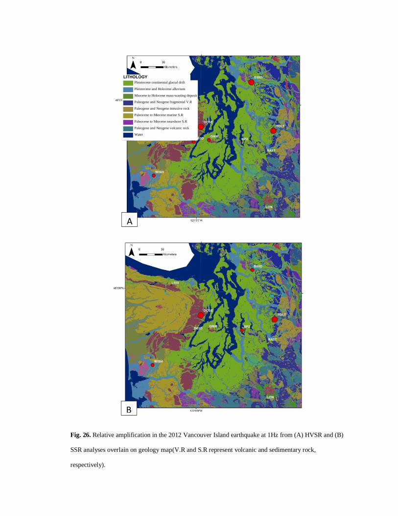
Fig. 26. Relative amplification in the 2012 Vancouver Island earthquake at 1Hz from (A) HVSR and (B)
SSR analyses overlain on geology map(V.R and S.R represent volcanic and sedimentary rock,
respectively).
A
B
Pleistocene continental glacial drift
Pleistocene and Holocene alluvium
Miocene to Holocene mass-wasting deposit
Paleogene and Neogene fragmental V.R
Paleogene and Neogene intrusive rock
Paleocene to Miocene marine S.R
Paleocene to Miocene nearshore S.R
Paleogene and Neogene volcanic rock
Water

Fig. 27. Relative amplification in the 2012 Vancouver Island earthquake (broadband data) at 3 Hz from
(A) HVSR and (B) SSR analyses overlain on geology map. Refer to Fig. 26 for legend.
A
B

Fig. 28. Relative amplification in the 2012 Vancouver Island earthquake (broadband data) at 5 Hz from (A)
HVSR and (B) SSR analyses overlain on geology map. Refer to Fig. 26 for legend.
A
B

Fig. 29. Relative amplification in the 2012 Vancouver Island earthquake (broadband data) at 7 Hz from (A)
HVSR and (B) SSR analyses overlain on geology map. Refer to Fig. 26 for legend.
A
B

Fig. 30. Relative amplification in the 2012 Vancouver Island earthquake (broadband data) at 9 Hz from (A)
HVSR and (B) SSR analyses overlain on geology map. Refer to Fig. 26 for legend.
A
B

According to the SSR results from the 2014 Vancouver Island earthquake (Figs.
31-35), the stations located on the Pleistocene continental glacial drift have high
amplification at 0-1.5 Hz and moderate amplification at 6-8 Hz. However, 3 out of 11
stations show low amplification at 0-1 Hz. High to moderate amplification at 1.5-10 Hz is
observed on the Paleogene and Neogene volcanic rock. Stations located on the
Pleistocene and Holocene alluvium have high amplification at 0.6-1.5 Hz and moderate
to low at 5-10 Hz.
Table 7. The maximum values of SSR and HVSR from the 2014 Vancouver Island earthquake at each
station in different frequencies.
Station
Name
1 Hz
SSR
3 Hz
SSR
5 Hz
SSR
7 Hz
SSR
9 Hz
SSR
1 Hz
HVSR
3 Hz
HVSR
5 Hz
HVSR
7 Hz
HVSR
9 Hz
HVSR
ALCT 22 13 17 14 8 3.5 2 4 3.3 2
ALKI 20 5 2 1 2 3 2 2 0.5 0.9
BEVT 65 14 13 8 16 6 1.7 1.9 1.6 2.3
DOSE 35 270 170 150 42 6.5 16.5 12 4.2 2.2
ELW 6 12 21 25 23 4 2 3.7 8 4
EVGW 220 60 42 30 20 5.1 1.5 1.2 0.8 0.8
FINN 18 13 18 4 2 5.5 1 3 3.5 1.5
KINR 45 53 75 30 18 3 6 8.5 6.8 1.5
LYNC 50 12 4 6 5 4 1.5 1.2 2 2.6
MARY 115 50 30 12 22 4.9 2.8 2 2.5 1.3
MEAN 60 50 35 12 165 5.7 5.5 5.5 1.7 0.7
NOWS 50 40 16 4 2 3.8 3.8 2 2.1 1.2

PAYL 51 57 36 43 30 4.5 10.5 10.5 1.8 1.1
PNLK 460 165 205 150 210 5.2 1.3 1.4 0.7 0.3
TOLT 62 38 40 47 44 16 10 2.6 3.5 7.5
CDMR 5 21 15 19 10 1.2 1.2 1.2 1.5 1.3
GNW - - - - - 1.2 1.5 2.2 3.4 2.5

Fig. 31. Relative amplification in the 2014 Vancouver Island earthquake at 1Hz from (A) HVSR and (B)
SSR analyses overlain on geology map(V.R and S.R represent volcanic and sedimentary rock,
respectively).
A
B
Pleistocene continental glacial drift
Pleistocene and Holocene alluvium
Miocene to Holocene mass-wasting deposit
Paleogene and Neogene fragmental V.R
Paleogene and Neogene intrusive rock
Paleocene to Miocene marine S.R
Paleocene to Miocene nearshore S.R
Paleogene and Neogene volcanic rock
Water

Fig. 32. Relative amplification in the 2014 Vancouver Island earthquake (strong motion data) at 3 Hz from
(A) HVSR and (B) SSR analyses overlain on geology map. Refer to Fig. 31 for legend.
A
B

Fig. 33. Relative amplification in the 2014 Vancouver Island earthquake (strong motion data) at 5 Hz from
(A) HVSR and (B) SSR analyses overlain on geology map. Refer to Fig. 31 for legend.
A
B

Fig. 34. Relative amplification in the 2014 Vancouver Island earthquake (strong motion data) at 7 Hz from
(A) HVSR and (B) SSR analyses overlain on geology map. Refer to Fig. 31 for legend.
A
B

Fig. 35. Relative amplification in the 2014 Vancouver Island earthquake (strong motion data) at 9 Hz from
(A) HVSR and (B) SSR analyses overlain on geology map. Refer to Fig. 31 for legend.
A
B

For the 2014 earthquake, 6 out of 9 stations located on the Pleistocene continental
glacial drift show relatively similar HVSR responses compared to the ones from SSRs.
They have high amplification at 0-1.5 Hz and 5-8 Hz. Likewise, the station on the
Paleogene and Neogene volcanic rock, has identical HVSR results compared to the SSR,
showing high amplification at 1-2 Hz and moderate at 3-10 Hz. Only half of the stations
on the Pleistocene and Holocene alluvium have similar HVSR and SSR results. In spite
of some inconsistencies between the results, they all agree on high amplification at 0-1
Hz and moderate to low amplification at 5-10 Hz. The station located on the Paleogene
and Neogene intrusive rock has relatively low amplification at 0-3 Hz and moderate at 4-
8 Hz. In general, 8 out of 16 stations have similar HVSR and SSR results in the 2014
Vancouver Island earthquake. 12 out of 24 in the 2012 Queen Charlotte earthquake, and 7
out of 8 in the 2012 Vancouver Island earthquake show similar results. Totally, 27 out of
48 (56%) of the stations have similar HVSR and SSR results for this earthquake.
Seattle Liquefaction Array (SLA)
SLA is a strong motion station that includes 4 accelerometers at different depths
from the surface (0 m, 5.4 m, 44.9 m, and 56.4 m). Shear-wave velocities at the site
linearly increase from ~100 m/s at the surface to ~250 m/s at a depth of 51 m. The
deepest accelerometer (56.4 m) is in material with Vs of approximately 400 m/s, which is
in Pleistocene and Holocene Pre-Vashon Deposits, with a transition zone above (51 m -
54 m) to material with Vs of 250 m/s (written communication, Jamison Steidl). The P
wave velocity at the depth of 2.5 km is estimated to be 2.5-3.5 km/s based on the

Fig. 36. Acceleration spectra of north and east components versus frequency at SLA from the 2012 Queen
Charlotte earthquake (strong motion data).The receivers are located at (A) 0 m (surface), (B) 5.4 m, (C)
44.9 m, and (D) 56.4 m. Notice that (A) and (B) show high amplifications while (C) and (D) are relatively
flat.
tomographic inversion of Van Wagoner et al. (2002). Due to the stiffness of the material
at the deepest accelerometer, the seismic recording at this depth was used as the reference
for the SSR calculations at this site. Figs. 36 and 37 show the spectra of the north and the
east components at different depths for the 2012 Queen Charlotte earthquake and the
2014 Vancouver Island earthquake, respectively. The spectra from the 2012 Queen
Charlotte earthquake are flat in the lower frequencies but show peaks at higher
frequencies (>7). The peaks are larger at shallower depths and weaker at deeper receiver
C D
B A

loations. The spectra from the 2014 Vancouver Island earthquake at shallow receivers
indicate peaks at low (0.5 to 1 Hz) and high (10 Hz) frequencies. The deeper receivers
however, show smaller peaks at the same frequencies.
Fig. 37. Acceleration spectra of north and east components versus frequency at SLA station from the 2014
Vancouver Island earthquake (strong motion data).The receivers are located as indicated in Fig. 36.
C D
B A
DISCUSSION
Previous studies have suggested that the age and the type of the geologic units and
the depth of the sediments to the bedrock are two major factors that determine the peak
frequencies and relative amplification observed in both SSR and the HVSR analyses
(Frankel, 1999; 2002; and 2009; Molnar et al. 2004; Pratt et al. 2006; Ghasemi et al.
2009; Koçkar and Akgün 2012). These two factors are investigated in this discussion. In
addition, results from the Seattle liquefaction array are used to explore the validity of the
SSR and HVSR methods.
Age and type of the geologic units
As reflected by the results shown in Figs 21-35, the SSRs from the three
earthquakes used in this study agree on high amplification at 1-1.5 Hz in areas underlain
by Pleistocene continental glacial drift. The HVSRs indicate a similar response for this
type of geology, with high amplification at 1-1.5 Hz.
The SSR results from the three earthquakes also show high amplification at 0.5-1
Hz for the stations located on the Pleistocene and Holocene alluvium. The HVSRs agree
with the SSRs to some extents. They suggest high to moderate amplification at 0-6 Hz.

These results agree with the results from Frankel et al. (2002) in which the highest
amplification was observed at 1 Hz on artificial fill and young alluvium.
All the HVSR and the SSR results for the station located at Paleocene to Miocene
marine sedimentary rock agree on low amplification at all frequencies. The same results
are observed for the single station located on the Paleogene and Neogene intrusive rock.
The SSRs agree on low amplification at 0-7 Hz and moderate at 7-10 Hz for the
stations located on the Paleogene and Neogene fragmental volcanic rock. The station on
the Paleogene and Neogene volcanic rock shows high amplification at 2-10 Hz according
to the SSRs. The HVSRs for this station suggests high amplification at 1-2 Hz. On the
average, the stations located on the Pleistocene and Holocene alluvium show the highest
amplification according to the HVSR results while the SSR results suggest Pleistocene
continental glacial drift as the type of geology with the highest amplification observed.
Overall there is a correlation between the observed peak frequencies and the type/age of
the geologic units.
Depth to the basement
Using results from the tomographic velocity inversion of Van Wagoner et al.,
2002 (Fig. 38) as a proxy for depth to basement, the correlation between the SSR and the
HVSR results and the depth to the basement is investigated for a few of the stations,
along with the correlation of SSR and HVSR results with the liquefaction susceptibility at
the sites. Figure 38 shows station locations used in this study overlain on a map of p-
wave velocities at a depth slice of 2.5 km. Basement is defined by the 4.25 km/s contour.

Areas having velocities less than 4.25 km at this depth are assumed to be above the basin-
basement interface.
MEAN is located in an urban area approximately at the center of the Seattle basin
on an area with the P wave velocity of 2.5-3 km/s at the depth of 2.5 km. The low P wave
velocity implies that this site is located in section of the basin that is deep and would
likely show amplification on the HVSR and the SSR results. However, very low
liquefaction susceptibility is suggested at this station according to the liquefaction
susceptibility map.
Moderate to high liquefaction susceptibility for NOWS is well justified by its low
P wave velocity (2.5-3 km/s) (located at the center of the basin) and the high
amplification at 1-3 Hz, as suggested by the HVSR and the SSR results. Located on the
Pleistocene and Holocene alluvium close to a river in a wide valley is consistent with
MARY’s designation of moderate to high liquefaction susceptibility and the high
amplification suggested by the SSR and the HVSR results at this station.
The station DOSE is located on the center of the valley on Pleistocene continental
glacial drift and consistently shows high amplification at 3-4 Hz in both the HVSR and
the SSR results from all the three events (Fig.38).In this regard, the SSR and HVSR
results are consistent with the assumption that both the type of geology and the depth to
basement are important factors governing the observed amplification at this site.
The relatively flat response on the SSR results for station FINN is consistent with
its very low liquefaction susceptibility for FINN. However, this station overlays thick
sediments, according to the velocity map (Fig. 38), near the center of the Seattle basin.

This might be caused by a rise or ridge in the subsurface structure in this part of the basin
that is too small to be resolved by the tomographic velocity inversion.
Located on basement rock, RATT and LON have consistently flat responses in
their SSR and HVSR results. The P wave velocity at the depth of 2.5 km is 5-6 km/s for
RATT, which is likely representative of igneous rock. Likewise, GNW and MNWA,
located on the Paleogene and Neogene intrusive rock and Paleocene to Miocene marine
sedimentary rock, respectively, have P wave velocities of 4.5-6 km/s and show no
amplification at any frequency.

Fig. 38. Horizontal depth slice showing P wave velocity in the depth of 2.5 km overlain with strong motion
station locations (modified from Van Wagoner et al., 2002). The shaded area is the 4.25 km/s contour line,
which is assumed to mark the basins’ boundaries and presence of basement rock.
4
4
TOLT, on the other hand, is located on the Paleogene and Neogene volcanic rock
and has a P wave velocity of 5-6 km/s, which suggests basement rock. However, it shows
consistent peaks at 1-2 Hz in its HVSR and SSR results. The possible reason that might
explain this inconsistency is the fact that this station is located on the flank of a steep
alluvial valley, which can reflect a complexity of structure or unconsolidated surface
deposit that could give rise to near-surface amplification.
Fig. 39 shows the calculated SSRs using the two shallowest accelerometers (0 m
and 5.4 m) referenced to the deepest one (56.4 m) for both the 2012 Queen Charlotte (A
and B) and 2014 Vancouver Island (C and D) earthquakes. The results show a flat
response at lower frequencies and relatively consistent peaks at 7 to 10 Hz. Notice (B)
and (D), which are the deeper receivers, have smaller peaks in comparison to those from
the receivers on the surface. This clearly indicates the increase in amplification in
shallower depths.

Fig. 39. SSR against frequency at SLA station referenced to the accelerometer located at the depth of
56.4m. (A) 0 m (surface) and (B) 5.4 m from the 2014 Vancouver Island earthquake. (C) 0 m (surface) and
(D) 5.4 m from the 2012 Queen Charlotte earthquake. Notice that (A) and (C) have higher peaks in
comparison to (B) and (D).
A similar comparison of the SSR results from the 2014 Vancouver earthquake and
the 2012 Queen Charlotte earthquake is shown in Fig. 39. Here, GNW is used as the
reference station used for the calculation. This station was chosen as a reference because
its acceleration spectra are flat across most frequencies (Fig. 40). As with the results
shown in Fig. 39, the SSRs from SLA calculated with GNW as a reference show
increased amplification with shallow depth (Fig. 40).
C D
B A

Fig. 40. SSR against frequency at SLA station referenced to GNW. (A) 0 m (surface) and (B) 5.4 m from
the 2014 Vancouver Island earthquake. (C) 0 m (surface) and (D) 5.4 m from the 2012 Queen Charlotte
earthquake.
Despite the slightly different peak frequencies in the spectra from the 2012 Queen
Charlotte earthquake and the 2014 Vancouver Island earthquake, which is possibly due to
the effect of source, the SSR peak frequencies are very consistent between the two
earthquakes and the results shows the method has successfully eliminated the effect of
the source.
C D
B A

The SSRs referenced to GNW also indicate higher amplification in the near
surface compared to deeper strata. The frequency peaks are somewhat consistent between
the two events. Although this result confirms the assumption that a different station can
be used as a reference site for the SSR calculation, the result is not fully consistent with
the results referenced to the deepest receiver at SLA. The fact that the deepest receiver at
SLA is still in stiff soil (and not bedrock) could be one reason for the inconsistency of the
SSR peak frequencies.

CONCLUSIONS
This study uses earthquake data to determine site effects, such as wave
amplification and frequency characteristics of ground motions, at several locations in
western Washington. It compares two common methodologies, SSR and HVSR, for
broadband and strong motion stations located in a variety of geologic settings.
The SSR and HVSR both show that the stations located on the Pleistocene
continental glacial drift show high amplification at 1-1.5 Hz.. Stations located on
Pleistocene and Holocene alluvium show relatively high amplification at 0.5-1
Hz.Stations on the Paleogene and Neogene intrusive rock and the Paleocene to Miocene
marine sedimentary rock show low amplification at all frequencies. Low amplification at
1-4 Hz a was observed for the only station located on the Paleogene and Neogene
fragmental volcanic rock.
Acquiring data from multiple depths (liquefaction array) is a practical approach to
study amplification characteristics that occur as a result of energy propagating through
near-surface basin sediments. The results from the liquefaction array show the degree and
frequency characteristics of near-surface wavesas energy travels through shallow layers,
and the consistency of the results when compared among multiple earthquakes supports
the validity of the technique.

In slightly more than half of the stations (56%), the HVSR and the SSR results
show relatively similar peaks. the HVSR method shows some inconsistencies with the
SSR and might not be a suitable method to estimate wave amplification in deep
sedimentary basins with complicated underlying structure. The SSR, on the other hand,
shows relatively more consistency, both within this study and with previous work done in
this area, suggesting that this is a useful method in evaluating areas susceptible to
liquefaction. However, it is suggested that the SSR method be used in conjunction with
other geophysical and geotechnical studies.

REFERENCES
Atkinson, G.M., 1995. Attenuation and source parameters of earthquakes in the Cascadia
region. Bulletin of the Seismological Society of America 85, 1327–1342.
Atwater, B.F., Musumi-Rokkaku, S., Satake, K., Tsuji, Y., Ueda, K., Yamaguchi, D.K., 2005.
The orphan tsunami of 1700; Japanese clues to a parent earthquake in North America. U.
S. Geological Survey Professional Paper 133.
Barnett, E.A., Weaver, C.S., Meagher, K.L., Haugerud, R.A., Wang, Z., Madin, I.P., Wang,
Y., Wells, R.E., Blakely, R.J., Ballantyne, D.B., Darienzo, M., 2009a. Earthquake
hazards and lifelines in the Interstate 5 urban corridor; Woodburn, Oregon, to Centralia,
Washington. Scientific Investigations Map 1 sheet.
Barnett, E.A., Weaver, C.S., Meagher, K.L., Haugerud, R.A., Wang, Z., Madin, I.P., Wang,
Y., Wells, R.E., Blakely, R.J., Ballantyne, D.B., Darienzo, M., 2009b. Earthquake
hazards and lifelines in the Interstate 5 urban corridor; Woodburn, Oregon, to Centralia,
Washington. Scientific Investigations Map 1 sheet.
Booth, D.B., 1994. Glaciofluvial infilling and scour of the Puget Lowland, Washington,
during ice-sheet glaciation. Geology (Boulder) 22, 695–698.
doi:http://dx.doi.org/10.1130/0091-7613(1994)022
Brocher, T.M., Parsons, T.E., Blakely, R.J., Christensen, N.I., Fisher, M.A., Wells, R.E., ten
Brink, U.S., Pratt, T.L., Crosson, R.S., Creager, K.C., Symons, N.P., Preston, L.A., Van
Wagoner, T., Miller, K.C., Snelson, C.M., Trehu, A.M., Langenheim, V.E., Spence,
G.D., Ramachandran, K., Hyndman, R.D., Mosher, D.C., Zelt, B.C., Weaver, C.S., 2001.
Upper crustal structure in Puget Lowland, Washington; results from the 1998 seismic

hazards investigation in Puget Sound. Journal of Geophysical Research 106, 13,541–
13,564.
Brocher, T.M., Parsons, T.E., Creager, K.C., Crosson, R.S., Symons, N.P., Spence, G.D., Zelt,
B.C., Hammer, P.T., Hyndman, R.D., Mosher, D.C., Trehu, A.M., Miller, K.C., ten
Brink, U.S., Fisher, M.A., Pratt, T.L., Alvarez, M.G., Beaudoin, B.C., Louden, K.E.,
Weaver, C.S., 1999. Wide-angle seismic recordings from the 1998 Seismic Hazards
Investigation of Puget Sound (SHIPS), western Washington and British Columbia. Open-
File Report - U. S. Geological Survey 110.
Fernandez, L.M., Brandt, M.B.C., 2000. The reference spectral noise ratio method to evaluate
the seismic response of a site. Soil Dynamics and Earthquake Engineering 20, 381–388.
doi:10.1016/S0267-7261(00)00086-5
Frankel, A., Stephenson, W., Carver, D., 2009. Sedimentary basin effects in Seattle,
Washington; ground-motion observations and 3D simulations. Bulletin of the
Seismological Society of America 99, 1579–1611.
doi:http://dx.doi.org/10.1785/0120080203
Frankel, A.D., Carver, D.L., Cranswick, E., Meremonte, M.E., Bice, T., Overturf, D.E., 1999.
Site response for Seattle and source parameters of earthquakes in the Puget Sound region.
Bulletin of the Seismological Society of America 89, 468–483.
Frankel, A.D., Carver, D.L., Williams, R.A., 2002. Nonlinear and linear site response and
basin effects in Seattle for the M 6.8 Nisqually, Washington, earthquake. Bulletin of the
Seismological Society of America 92, 2090–2109.
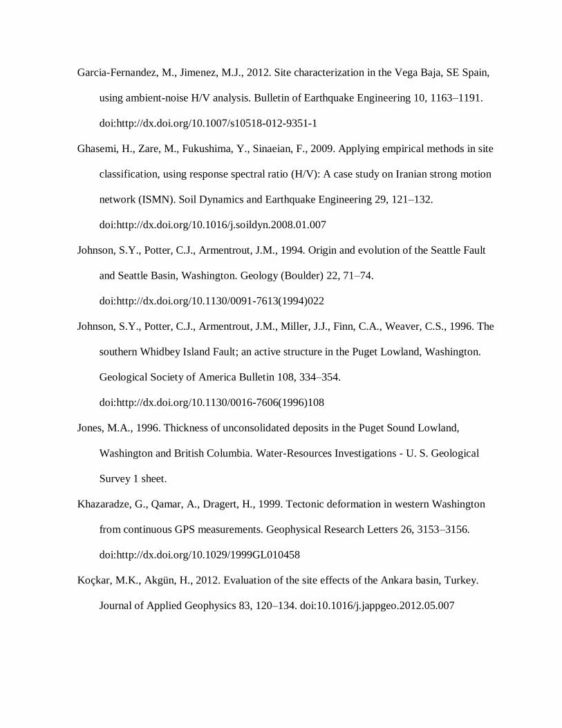
Garcia-Fernandez, M., Jimenez, M.J., 2012. Site characterization in the Vega Baja, SE Spain,
using ambient-noise H/V analysis. Bulletin of Earthquake Engineering 10, 1163–1191.
doi:http://dx.doi.org/10.1007/s10518-012-9351-1
Ghasemi, H., Zare, M., Fukushima, Y., Sinaeian, F., 2009. Applying empirical methods in site
classification, using response spectral ratio (H/V): A case study on Iranian strong motion
network (ISMN). Soil Dynamics and Earthquake Engineering 29, 121–132.
doi:http://dx.doi.org/10.1016/j.soildyn.2008.01.007
Johnson, S.Y., Potter, C.J., Armentrout, J.M., 1994. Origin and evolution of the Seattle Fault
and Seattle Basin, Washington. Geology (Boulder) 22, 71–74.
doi:http://dx.doi.org/10.1130/0091-7613(1994)022
Johnson, S.Y., Potter, C.J., Armentrout, J.M., Miller, J.J., Finn, C.A., Weaver, C.S., 1996. The
southern Whidbey Island Fault; an active structure in the Puget Lowland, Washington.
Geological Society of America Bulletin 108, 334–354.
doi:http://dx.doi.org/10.1130/0016-7606(1996)108
Jones, M.A., 1996. Thickness of unconsolidated deposits in the Puget Sound Lowland,
Washington and British Columbia. Water-Resources Investigations - U. S. Geological
Survey 1 sheet.
Khazaradze, G., Qamar, A., Dragert, H., 1999. Tectonic deformation in western Washington
from continuous GPS measurements. Geophysical Research Letters 26, 3153–3156.
doi:http://dx.doi.org/10.1029/1999GL010458
Koçkar, M.K., Akgün, H., 2012. Evaluation of the site effects of the Ankara basin, Turkey.
Journal of Applied Geophysics 83, 120–134. doi:10.1016/j.jappgeo.2012.05.007

Mahajan, A.K., Mundepi, A.K., Chauhan, N., Jasrotia, A.S., Rai, N., Gachhayat, T.K., 2012.
Active seismic and passive microtremor HVSR for assessing site effects in Jammu city,
NW Himalaya, India—A case study. Journal of Applied Geophysics 77, 51–62.
doi:10.1016/j.jappgeo.2011.11.005
Microtremor measurements in the northern coast of İzmir Bay, Turkey to evaluate site-specific
characteristics and fundamental periods by H/V spectral ratio method - Springer, n.d.
Molnar, S., Cassidy, J.F., Dosso, S.E., 2004. Site response in Victoria, British Columbia from
spectral ratios and 1D modeling. Bulletin of the Seismological Society of America 94,
1109–1124.
Palmer, S., Magsino, S., Bilderback, E., Poelstra, J., Folger, D., Niggemann, R., 2004.
Liquefaction Susceptibility and Site Class Maps of Washington State, by County.
Pratt, T.L., 2006. Site response, basin effects, and attenuation in the Puget Lowland,
Washington State, U. S. Bulletin of the Earthquake Research Institute = Tokyo Daigaku
Jishin Kenkyusho Iho 81, 283–289.
Pratt, T.L., Brocher, T.M., Anonymous, 2003. Basin attenuation and the characteristics of
simple spectral ratio and H/V site response estimates. Eos, Transactions, American
Geophysical Union 84, F1041.
Pratt, T.L., Brocher, T.M., Weaver, C.S., Miller, K.C., Trehu, A.M., Creager, K.C., Crosson,
R.S., Anonymous, 2000. Amplification of seismic waves by the Seattle Basin,
Washington State. Eos, Transactions, American Geophysical Union 81, 827.
Snelson, C.M., Brocher, T.M., Miller, K.C., Pratt, T.L., Trehu, A.M., 2007. Seismic
amplification within the Seattle Basin, Washington State; insights from SHIPS seismic

tomography experiments. Bulletin of the Seismological Society of America 97, 1432–
1448. doi:http://dx.doi.org/10.1785/0120050204
Troost, K.G., Booth, D.B., 2008. Geology of Seattle and the Seattle area, Washington.
Reviews in Engineering Geology 20, 1–35. doi:http://dx.doi.org/10.1130/2008.4020(01
Van Wagoner, T.M., Crosson, R.S., Creager, K.C., Medema, G.F., Preston, L.A., Symons,
N.P., Brocher, T.M., 2002. Crustal structure and relocated earthquakes in the Puget
Lowland, Washington, from high-resolution seismic tomography. Journal of Geophysical
Research 107, 23. doi:http://dx.doi.org/10.1029/2001JB000710

APPENDICES
Appendix A
The north, east, and vertical components of spectra for strong motion data from
2014 Vancouver Island earthquake relative to the surface geology at the station locations.
1) Pleistocene continental glacial drift


2) Paleogene and Neogene volcanic rock
3) Pleistocene and Holocene alluvium

4) Paleogene and Neogene intrusive rock

Appendix B
The north, east, and vertical components of spectra for broadband data from 2012
Vancouver Island earthquake relative to the surface geology at the station locations.
1) Pleistocene continental glacial drift

1) Paleogene and Neogene volcanic rock
2) Pleistocene and Holocene alluvium
3) Paleogene and Neogene intrusive rock

4) Paleogene and Neogene fragmental volcanic rock
Appendix C
The north, east, and vertical components of spectra for strong motion data from
2012 Queen Charlotte earthquake relative to the surface geology at the station locations.
1) Pleistocene continental glacial drift


2) Paleogene and Neogene volcanic rock
3) Pleistocene and Holocene alluvium

4) Paleogene and Neogene fragmental volcanic rock

5) Paleocene to Miocene marine sedimentary rock
6) Paleogene and Neogene intrusive rock

Appendix D
MATLAB codes used to calculate the HVSRs for 2014 Vancouver Island
Earthquake strong motion data.
% Script to calculate and plot the HVSR for 2014 Vancouver Island
% earthquake strong motion data
echo off
%
nfft=1024;
noverlap=nfft/2;
prob=.95;
%traveltime and radial distance
t=67.6;
r=465.2387224;
%Selecting a window that starts before S-wave and continues for 7001
%samples
LOCUT = 69000;
HICUT = 76000;
% load multicomponent sac files
[sachdrE,data2E] = load_sac('ALCT.UW..ENE.2014.114.03.00.00.000-
2014.114.03.39.59.999.scale-AUTO.sac');
[sachdrN,data2N] = load_sac('ALCT.UW..ENN.2014.114.03.00.00.000-
2014.114.03.39.59.999.scale-AUTO.sac');
[sachdrZ,data2Z] = load_sac('ALCT.UW..ENZ.2014.114.03.00.00.000-
2014.114.03.40.00.000.scale-AUTO.sac');
% Applying the filter
[data2Z]=bandpass(data2Z,0.2,25,7001,0.01);
[data2E]=bandpass(data2E,0.2,25,7001,0.01);
[data2N]=bandpass(data2N,0.2,25,7001,0.01);
%cut the data
data2E = data2E(LOCUT:HICUT);

data2N = data2N(LOCUT:HICUT);
data2Z = data2Z(LOCUT:HICUT);
% demean and detrend the time segment
data2E = detrend(data2E-mean(data2E));
data2N = detrend(data2N-mean(data2N));
data2Z = detrend(data2Z-mean(data2Z));
% create Hann taper the length of your data
w = hann(length(data2E));
% taper the data
data2E = data2E.*w;
data2N = data2N.*w;
data2Z = data2Z.*w;
%Calculating the Power Spectral Density
% Vertical Component
dt=1.0/sachdrZ.delta;
[Pmz,Fmz]=psd(data2Z,nfft,dt,[],noverlap,prob);
%East Component
dt=1.0/sachdrE.delta;
[Pme,Fmz]=psd(data2E,nfft,dt,[],noverlap,prob);
%North Component
dt=1.0/sachdrN.delta;
[Pmn,Fmz]=psd(data2N,nfft,dt,[],noverlap,prob);
%Attenuation Correction
Pmz_corr=Pmz.*(r^0.5).*exp(pi.*(Fmz.^0.61).*t/380);
Pmn_corr=Pmn.*(r^0.5).*exp(pi.*(Fmz.^0.61).*t/380);
Pme_corr=Pme.*(r^0.5).*exp(pi.*(Fmz.^0.61).*t/380);
% Calculating the HVSR
ratmiMT=(Pme_corr+Pmn_corr)./(2.0.*Pmz_corr);
%smoothing
ratmiMT1=smooth(ratmiMT,10);

%Plotting
semilogx(Fmz,ratmiMT1,'k')
title ('ALCT')
ylabel ('H/V')
xlabel ('frequency (Hz)')
set(gca,'xlim',[0,10],'ylim',[0,8])
MATLAB codes used to calculate the HVSRs for 2012 Vancouver Island Earthquake
broadband data.
% Script to calculate and plot the HVSR for 2012 Vancouver Island
% earthquake broadband data
echo off
%
nfft=512;
noverlap=nfft/2;
prob=.95;
%traveltime and radial distance
t=64;
r=480.0804502;
%Selecting a window that starts before S-wave and continues for 3001
%samples
LOCUT = 31800;
HICUT = 34800;
% load multicomponent sac files
[sachdrE,data2E] = load_sac('B05D.TA..BHE.2012.313.01.50.00.000-
2012.313.02.30.00.000.scale-AUTO.sac');
[sachdrN,data2N] = load_sac('B05D.TA..BHN.2012.313.01.50.00.000-
2012.313.02.30.00.000.scale-AUTO.sac');
[sachdrZ,data2Z] = load_sac('B05D.TA..BHZ.2012.313.01.50.00.000-
2012.313.02.29.59.999.scale-AUTO.sac');

% Applying the filter
[data2Z]=bandpass(data2Z,0.2,15,3001,0.025);
[data2E]=bandpass(data2E,0.2,15,3001,0.025);
[data2N]=bandpass(data2N,0.2,15,3001,0.025);
%cut the data
data2E = data2E(LOCUT:HICUT);
data2N = data2N(LOCUT:HICUT);
data2Z = data2Z(LOCUT:HICUT);
% demean and detrend the time segment
data2E = detrend(data2E-mean(data2E));
data2N = detrend(data2N-mean(data2N));
data2Z = detrend(data2Z-mean(data2Z));
%create Hann taper the length of your data
w = hann(length(data2E));
% taper the data
data2E = data2E.*w;
data2N = data2N.*w;
data2Z = data2Z.*w;
%Calculating the Power Spectral Density
% Vertical Component
dt=1.0/sachdrZ.delta;
[Pmz,Fmz]=psd(data2Z,nfft,dt,[],noverlap,prob);
%East Component
dt=1.0/sachdrE.delta;
[Pme,Fmz]=psd(data2E,nfft,dt,[],noverlap,prob);
%North Component
dt=1.0/sachdrN.delta;
[Pmn,Fmz]=psd(data2N,nfft,dt,[],noverlap,prob);
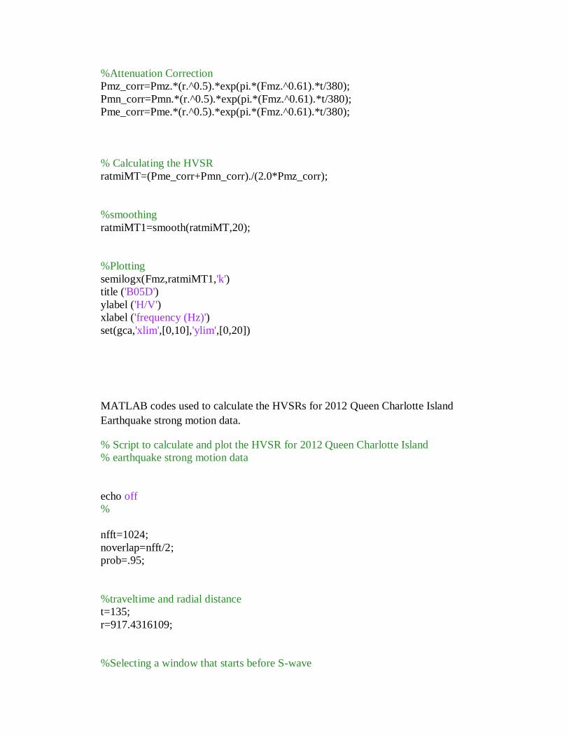
%Attenuation Correction
Pmz_corr=Pmz.*(r.^0.5).*exp(pi.*(Fmz.^0.61).*t/380);
Pmn_corr=Pmn.*(r.^0.5).*exp(pi.*(Fmz.^0.61).*t/380);
Pme_corr=Pme.*(r.^0.5).*exp(pi.*(Fmz.^0.61).*t/380);
% Calculating the HVSR
ratmiMT=(Pme_corr+Pmn_corr)./(2.0*Pmz_corr);
%smoothing
ratmiMT1=smooth(ratmiMT,20);
%Plotting
semilogx(Fmz,ratmiMT1,'k')
title ('B05D')
ylabel ('H/V')
xlabel ('frequency (Hz)')
set(gca,'xlim',[0,10],'ylim',[0,20])
MATLAB codes used to calculate the HVSRs for 2012 Queen Charlotte Island
Earthquake strong motion data.
% Script to calculate and plot the HVSR for 2012 Queen Charlotte Island
% earthquake strong motion data
echo off
%
nfft=1024;
noverlap=nfft/2;
prob=.95;
%traveltime and radial distance
t=135;
r=917.4316109;
%Selecting a window that starts before S-wave

LOCUT = 101000;
HICUT = 108000;
% load multicomponent sac files
[sachdrE,data2E] = load_sac('ALCT.UW..ENE.2012.302.02.50.00.000-
2012.302.03.30.00.000.scale-AUTO.sac');
[sachdrN,data2N] = load_sac('ALCT.UW..ENN.2012.302.02.50.00.000-
2012.302.03.30.00.000.scale-AUTO.sac');
[sachdrZ,data2Z] = load_sac('ALCT.UW..ENZ.2012.302.02.50.00.000-
2012.302.03.30.00.000.scale-AUTO.sac');
% Applying the filter
[data2Z]=bandpass(data2Z,0.2,25,7001,0.01);
[data2E]=bandpass(data2E,0.2,25,7001,0.01);
[data2N]=bandpass(data2N,0.2,25,7001,0.01);
%cut the data
data2E = data2E(LOCUT:HICUT);
data2N = data2N(LOCUT:HICUT);
data2Z = data2Z(LOCUT:HICUT);
% demean and detrend the time segment
data2E = detrend(data2E-mean(data2E));
data2N = detrend(data2N-mean(data2N));
data2Z = detrend(data2Z-mean(data2Z));
% create Hann taper the length of your data
w = hann(length(data2E));
% taper the data
data2E = data2E.*w;
data2N = data2N.*w;
data2Z = data2Z.*w;
%Calculating the Power Spectral Density
% Vertical Component
dt=1.0/sachdrZ.delta;
[Pmz,Fmz]=psd(data2Z,nfft,dt,[],noverlap,prob);
%East Component

dt=1.0/sachdrE.delta;
[Pme,Fmz]=psd(data2E,nfft,dt,[],noverlap,prob);
%North Component
dt=1.0/sachdrN.delta;
[Pmn,Fmz]=psd(data2N,nfft,dt,[],noverlap,prob);
%Attenuation Correction
Pmz_corr=Pmz.*(r^0.5).*exp(pi.*(Fmz.^0.61).*t/380);
Pmn_corr=Pmn.*(r^0.5).*exp(pi.*(Fmz.^0.61).*t/380);
Pme_corr=Pme.*(r^0.5).*exp(pi.*(Fmz.^0.61).*t/380);
% Calculating the HVSR
ratmiMT=(Pme_corr+Pmn_corr)./(2.0*Pmz_corr);
%smoothing
ratmiMT1=smooth(ratmiMT,10);
%Plotting
semilogx(Fmz,ratmiMT1,'k')
title ('ALCT')
ylabel ('H/V')
xlabel ('frequency (Hz)')
set(gca,'xlim',[0,10],'ylim',[0,8])
MATLAB codes used to calculate the SSRs for 2014 Vancouver Island Earthquake
strong motion data.
% Script to calculate and plot the SSR for 2014 Vancouver Island
% earthquake strong motion data referenced to GNW and CDMR stations
echo off
%
nfft=1024;
noverlap=nfft/2;
prob=.95;

%traveltime and radial distance
t=67.6;
r=465.2387224;
%Selecting a window that starts before S-wave and continues for 7001
%samples
LOCUT = 69000;
HICUT = 76000;
% load multicomponent sac files
[sachdrE,data2E] = load_sac('ALCT.UW..ENE.2014.114.03.00.00.000-
2014.114.03.39.59.999.scale-AUTO.sac');
[sachdrN,data2N] = load_sac('ALCT.UW..ENN.2014.114.03.00.00.000-
2014.114.03.39.59.999.scale-AUTO.sac');
% Applying the filter
[data2E]=bandpass(data2E,0.2,25,7001,0.01);
[data2N]=bandpass(data2N,0.2,25,7001,0.01);
%cut the data
data2E = data2E(LOCUT:HICUT);
data2N = data2N(LOCUT:HICUT);
% demean and detrend the time segment
data2E = detrend(data2E-mean(data2E));
data2N = detrend(data2N-mean(data2N));
% create Hann taper the length of your data
w = hann(length(data2E));
% taper the data
data2E = data2E.*w;
data2N = data2N.*w;
%Calculating the Power Spectral Density
%East Component

dt=1.0/sachdrE.delta;
[Pme,Fmz]=psd(data2E,nfft,dt,[],noverlap,prob);
%North Component
dt=1.0/sachdrN.delta;
[Pmn,Fmz]=psd(data2N,nfft,dt,[],noverlap,prob);
%Attenuation Correction
Pmn_corr=Pmn.*(r^0.5).*exp(pi.*(Fmz.^0.61).*t/380);
Pme_corr=Pme.*(r^0.5).*exp(pi.*(Fmz.^0.61).*t/380);
% Calculating the average
ratmiMT=(Pme_corr+Pmn_corr)./(2.0);
%Calculating the reference site "GNW"
%traveltime and radial distance
t=56.3;
r=497.0186862;
%traveltime and radial distance
t=71.1;
r=404.0315121;
%Selecting a window that starts before S-wave
LOCUT = 67830;
HICUT = 74830;
% load multicomponent sac files
[sachdrE,data2E] = load_sac('GNW.UW..ENE.2014.114.03.00.00.005-
2014.114.03.39.59.995.bp-0.01-25.scale-AUTO.sac');
[sachdrN,data2N] = load_sac('GNW.UW..ENN.2014.114.03.00.00.005-
2014.114.03.39.59.994.bp-0.01-25.scale-AUTO.sac');
% Applying the filter
[data2E]=bandpass(data2E,0.2,25,7001,0.01);
[data2N]=bandpass(data2N,0.2,25,7001,0.01);

%cut the data
data2E = data2E(LOCUT:HICUT);
data2N = data2N(LOCUT:HICUT);
% demean and detrend the time segment
data2E = detrend(data2E-mean(data2E));
data2N = detrend(data2N-mean(data2N));
% create Hann taper the length of your data
w = hann(length(data2E));
% taper the data
data2E = data2E.*w;
data2N = data2N.*w;
%Calculating the Power Spectral Density
%East Component
dt=1.0/sachdrE.delta;
[Pme,Fmz]=psd(data2E,nfft,dt,[],noverlap,prob);
%North Component
dt=1.0/sachdrN.delta;
[Pmn,Fmz]=psd(data2N,nfft,dt,[],noverlap,prob);
%Attenuation Correction
Pmn_corr=Pmn.*(r^0.5).*exp(pi.*(Fmz.^0.61).*t/380);
Pme_corr=Pme.*(r^0.5).*exp(pi.*(Fmz.^0.61).*t/380);
% Calculating the average
ratmiMTGNW=(Pme_corr+Pmn_corr)./(2.0);
% Calculating the ratio
ratmiMT1=ratmiMT./ratmiMTGNW;
%smoothing
ratmiMT1GNW=smooth(ratmiMT1,10);
%Plotting
semilogx(Fmz,ratmiMT1GNW,'k')

title ('ALCT')
ylabel ('SSR')
xlabel ('frequency (Hz)')
set(gca,'xlim',[0,10],'ylim',[0,100])
MATLAB codes used to calculate the SSRs for 2012 Vancouver Island Earthquake
broadband data.
% Script to calculate and plot the SSR for 2012 Vancouver Island
% earthquake broadband data
echo off
%
nfft=512;
noverlap=nfft/2;
prob=.95;
%traveltime and radial distance
t=64;
r=480.0804502;
%Selecting a window that starts before S-wave and continues for 3001
%samples
LOCUT = 31800;
HICUT = 34800;
% load multicomponent sac files
[sachdrE,data2E] = load_sac('B05D.TA..BHE.2012.313.01.50.00.000-
2012.313.02.30.00.000.scale-AUTO.sac');
[sachdrN,data2N] = load_sac('B05D.TA..BHN.2012.313.01.50.00.000-
2012.313.02.30.00.000.scale-AUTO.sac');
% Applying the filter
[data2E]=bandpass(data2E,0.2,15,3001,0.025);
[data2N]=bandpass(data2N,0.2,15,3001,0.025);
%cut the data
data2E = data2E(LOCUT:HICUT);
data2N = data2N(LOCUT:HICUT);

% demean and detrend the time segment
data2E = detrend(data2E-mean(data2E));
data2N = detrend(data2N-mean(data2N));
% create Hann taper the length of your data
w = hann(length(data2E));
% taper the data
data2E = data2E.*w;
data2N = data2N.*w;
%Calculating the Power Spectral Density
%East Component
dt=1.0/sachdrE.delta;
[Pme,Fmz]=psd(data2E,nfft,dt,[],noverlap,prob);
%North Component
dt=1.0/sachdrN.delta;
[Pmn,Fmz]=psd(data2N,nfft,dt,[],noverlap,prob);
%Attenuation Correction
Pmn_corr=Pmn.*(r.^0.5).*exp(pi.*(Fmz.^0.61).*t/380);
Pme_corr=Pme.*(r.^0.5).*exp(pi.*(Fmz.^0.61).*t/380);
% Calculating the average
ratmiMT=(Pme_corr+Pmn_corr)./(2.0);
%traveltime and radial distance
t=60.75;
r=463.714543;
%Selecting a window that starts before S-wave
LOCUT = 31800;
HICUT = 34800;
% load multicomponent sac files
[sachdrE,data2E] = load_sac('GNW.UW..BHE.2012.313.01.50.00.015-
2012.313.02.29.59.990.scale-AUTO.sac');
[sachdrN,data2N] = load_sac('GNW.UW..BHN.2012.313.01.50.00.015-
2012.313.02.29.59.989.scale-AUTO.sac');

% Applying the filter
[data2E]=bandpass(data2E,0.2,15,3001,0.025);
[data2N]=bandpass(data2N,0.2,15,3001,0.025);
%cut the data
data2E = data2E(LOCUT:HICUT);
data2N = data2N(LOCUT:HICUT);
% demean and detrend the time segment
data2E = detrend(data2E-mean(data2E));
data2N = detrend(data2N-mean(data2N));
% create Hann taper the length of your data
w = hann(length(data2E));
% taper the data
data2E = data2E.*w;
data2N = data2N.*w;
%Calculating the Power Spectral Density
%East Component
dt=1.0/sachdrE.delta;
[Pme,Fmz]=psd(data2E,nfft,dt,[],noverlap,prob);
%North Component
dt=1.0/sachdrN.delta;
[Pmn,Fmz]=psd(data2N,nfft,dt,[],noverlap,prob);
%Attenuation Correction
Pmn_corr=Pmn.*(r^0.5).*exp(pi.*(Fmz.^0.61).*t/380);
Pme_corr=Pme.*(r^0.5).*exp(pi.*(Fmz.^0.61).*t/380);
% Calculating the average
ratmiMTGNW=(Pme_corr+Pmn_corr)./(2.0);
ratmiMT1=ratmiMT./ratmiMTGNW;
%smoothing
ratmiMT1=smooth(ratmiMT1,20);

%Plotting
semilogx(Fmz,ratmiMT1,'k')
title ('B05D')
ylabel ('SSR')
xlabel ('frequency (Hz)')
set(gca,'xlim',[0,10],'ylim',[0,100])
MATLAB codes used to calculate the SSRs for 2012 Queen Charlotte Island Earthquake
strong motion data.
% Script to calculate and plot the SSR for 2012 Vancouver Island
% earthquake broadband data
echo off
%
nfft=512;
noverlap=nfft/2;
prob=.95;
%traveltime and radial distance
t=64;
r=480.0804502;
%Selecting a window that starts before S-wave and continues for 3001
%samples
LOCUT = 31800;
HICUT = 34800;
% load multicomponent sac files
[sachdrE,data2E] = load_sac('B05D.TA..BHE.2012.313.01.50.00.000-
2012.313.02.30.00.000.scale-AUTO.sac');
[sachdrN,data2N] = load_sac('B05D.TA..BHN.2012.313.01.50.00.000-
2012.313.02.30.00.000.scale-AUTO.sac');
% Applying the filter
[data2E]=bandpass(data2E,0.2,15,3001,0.025);
[data2N]=bandpass(data2N,0.2,15,3001,0.025);
%cut the data

data2E = data2E(LOCUT:HICUT);
data2N = data2N(LOCUT:HICUT);
% demean and detrend the time segment
data2E = detrend(data2E-mean(data2E));
data2N = detrend(data2N-mean(data2N));
% create Hann taper the length of your data
w = hann(length(data2E));
% taper the data
data2E = data2E.*w;
data2N = data2N.*w;
%Calculating the Power Spectral Density
%East Component
dt=1.0/sachdrE.delta;
[Pme,Fmz]=psd(data2E,nfft,dt,[],noverlap,prob);
%North Component
dt=1.0/sachdrN.delta;
[Pmn,Fmz]=psd(data2N,nfft,dt,[],noverlap,prob);
%Attenuation Correction
Pmn_corr=Pmn.*(r.^0.5).*exp(pi.*(Fmz.^0.61).*t/380);
Pme_corr=Pme.*(r.^0.5).*exp(pi.*(Fmz.^0.61).*t/380);
% Calculating the average
ratmiMT=(Pme_corr+Pmn_corr)./(2.0);
%traveltime and radial distance
t=60.75;
r=463.714543;
%Selecting a window that starts before S-wave
LOCUT = 31800;
HICUT = 34800;
% load multicomponent sac files
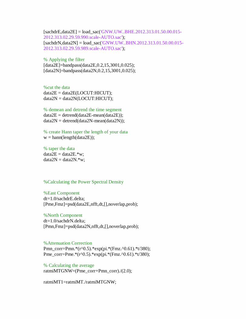
[sachdrE,data2E] = load_sac('GNW.UW..BHE.2012.313.01.50.00.015-
2012.313.02.29.59.990.scale-AUTO.sac');
[sachdrN,data2N] = load_sac('GNW.UW..BHN.2012.313.01.50.00.015-
2012.313.02.29.59.989.scale-AUTO.sac');
% Applying the filter
[data2E]=bandpass(data2E,0.2,15,3001,0.025);
[data2N]=bandpass(data2N,0.2,15,3001,0.025);
%cut the data
data2E = data2E(LOCUT:HICUT);
data2N = data2N(LOCUT:HICUT);
% demean and detrend the time segment
data2E = detrend(data2E-mean(data2E));
data2N = detrend(data2N-mean(data2N));
% create Hann taper the length of your data
w = hann(length(data2E));
% taper the data
data2E = data2E.*w;
data2N = data2N.*w;
%Calculating the Power Spectral Density
%East Component
dt=1.0/sachdrE.delta;
[Pme,Fmz]=psd(data2E,nfft,dt,[],noverlap,prob);
%North Component
dt=1.0/sachdrN.delta;
[Pmn,Fmz]=psd(data2N,nfft,dt,[],noverlap,prob);
%Attenuation Correction
Pmn_corr=Pmn.*(r^0.5).*exp(pi.*(Fmz.^0.61).*t/380);
Pme_corr=Pme.*(r^0.5).*exp(pi.*(Fmz.^0.61).*t/380);
% Calculating the average
ratmiMTGNW=(Pme_corr+Pmn_corr)./(2.0);
ratmiMT1=ratmiMT./ratmiMTGNW;

%smoothing
ratmiMT1=smooth(ratmiMT1,20);
%Plotting
semilogx(Fmz,ratmiMT1,'k')
title ('B05D')
ylabel ('SSR')
xlabel ('frequency (Hz)')
set(gca,'xlim',[0,10],'ylim',[0,100])
Appendix E
Geological Society of America (GSA) geologic time scale.
`