a comparative study of optimization techniques for …

International Journal of Management, IT & Engineering Vol. 9 Issue 7, July 2019,

ISSN: 2249-0558 Impact Factor: 7.119

Journal Homepage: http://www.ijmra.us, Email: [email protected]

Double-Blind Peer Reviewed Refereed Open Access International Journal - Included in the International Serial

Directories Indexed & Listed at: Ulrich's Periodicals Directory ©, U.S.A., Open J-Gage as well as in Cabell‟s

Directories of Publishing Opportunities, U.S.A

195 International journal of Management, IT and Engineering

http://www.ijmra.us, Email: [email protected]

A COMPARATIVE STUDY OF OPTIMIZATION

TECHNIQUES FOR VOLTAGE STABILITY OF POWER

SYSTEM

Dhruvi Chopra

Prof. Y. D. Shahakar

Abstract

Present day power systems are being operated closer to their

stability limits due to economic constraints. In today‟s scenario, as

the development is taking place simultaneously the demand for the

electricity in the world is also increasing. Operation and planning of

large interconnected power systems are becoming more and more

complex. In power system, voltage stability plays a very important

role. Voltage instability may cause blackouts and collapse of the

power system. Maintaining a stable and secure operation of a power

system is therefore very important and challenging issue. Many

traditional and advanced optimization techniques have been

proposed for reactive power dispatch to improve voltage stability of

the power system. In this paper, the importance of voltage stability

and optimal reactive power dispatch are discussed and analysis of

voltage stability is carried out using L–index method. The different

optimization techniques for improving voltage stability are studied.

This paper presents LP and PSO algorithm for system parameters

development for enhancing voltage stability and voltage profile

improvement. All algorithms are tested in IEEE 39 bus system. The

performance of PSO is compared with conventional linear

programming methods.

Keywords:

Voltage Stability;

Linear Programming;

PSO;

Voltage Profile

Improvement;

L-index.

M.E. (EPS), P.R.Pote COE & M, Amravati

Assistant Professor, Department of Electrical Engineering, P.R. Pote COE & M,

Amravati




1. Introduction

Voltage stability refers to the ability of power system to maintain steady voltages at all the buses

in the system after being subjected to a disturbance from a given initial operating point. The

system state enters the voltage instability region when a disturbance or an increase in load

demand or alteration in system state results in an uncontrollable and continuous drop in system

voltage. Enhancing the voltage stability indirectly means reactive power control. Any changes in

either power demand or system configuration implies increase or decrease in voltage. These

changes can lead to system instability which can be improved through reactive power allocation.

Reactive power allocation can be done by (a) tap changing transformer (b) changing generator

voltages (c) switchable var sources. The optimal reactive power control problem can be stated as

the problem of finding the correct value control variables so that the loss can be decreased. The

main advantages of reactive power control are decrease in transmission losses, increase in power

transmission capability, improved voltage profile and improved system stability. To obtain

optimized reactive power control different objective functions are optimized like to minimize the

sum of square of the voltage deviations of the load buses, minimization of sum of squares of

voltage stability L indices of load buses, real power loss minimization, etc. To optimize we use

different techniques like PSO, Genetic Algorithm, Fuzzy Logic, Linear Programming, etc. The

process of improving something than its current condition is called as Optimization. It is the

process of adjusting inputs, mathematical process or device characteristics to get the required

output. This process is called as fitness function, objective function or cost function. Particle

Swarm Optimization is inspired by behaviour of bird flocking. This algorithm consists of swarm

of particles i.e. group of random particles where each single solution is a bird (particle) in the

search space. Optimized solution for every particle is determined by fitness function. PSO is

based on birds swarm searching for optimal food sources in which direction of birds movement

is influenced by its current movement. Linear programming is a simple technique where

we depict complex relationships through linear functions and then find the optimum points. The

real relationships might be much more complex – but we can simplify them to linear

relationships. Linear programming is used for obtaining the most optimal solution for a problem

with given constraints. In linear programming, we formulate our real life problem into a

mathematical model. It involves an objective function, linear inequalities with subject to

constraints.




Linear programming is adaptive and more flexibility to analyze the problems. The main

advantage of linear programming is its simplicity and easy way of understanding. Linear

Programming (LP) is a technique for optimization of a linear objective function, subject to linear

equality and linear inequality constraints. The linear programming approach is based on an

assumption that the world is linear. In the real world, this is not always the case. Therefore LP

Technique cannot be used as efficient method of optimization. Particle Swarm Optimization

characterized into the domain of Artificial Intelligence. The term „Artificial Intelligence‟ or

„Artificial Life‟ refers to the theory of simulating human behaviour through computation. It

involves designing such computer systems which are able to execute tasks which require human

intelligence. PSO technique allows greater diversity and exploration over a single population.

Classical optimization techniques such as LP and NLP are efficient approaches that can be used

to solve special cases of optimization problem in power system applications. As the complexities

of the problem increase, especially with the introduction of uncertainties to the system, more

complicated optimization techniques, such as stochastic programming have to be used. Particle

Swarm Optimization (PSO) technique can be an alternative solution for these complex problems.

PSO is characterized as simple in concept easy to implement, and computationally efficient. PSO

has a flexible and well-balanced mechanism to enhance and adapt to the global and local

exploration abilities. Moreover it allows faster convergence and requires least computation time.

Therefore in this paper the main objective is to prove that PSO is best optimization method

compared to traditional LP Technique.

In this paper a mathematical model is developed for optimization techniques and minute changes

in the system are observed after the increment of load. The voltage stability is enhanced by

performing optimization in objective functions. This optimization will help to find the suitable

control variables settings for the power system. The results obtain are compared with traditional

and advanced technique.

2. L-index method and voltage stability analysis

The objectives in the proposed system is to minimize the sum of squares of voltage

stability L-indices of load buses (ΣL2) and analysis of this objective function is presented to

http://en.wikipedia.org/wiki/Optimization_%28mathematics%29

http://en.wikipedia.org/wiki/Linear

http://en.wikipedia.org/wiki/Objective_function

http://en.wikipedia.org/wiki/Linear_equality



http://en.wikipedia.org/wiki/Linear_inequality

http://en.wikipedia.org/wiki/Constraint_%28mathematics%29




illustrate the advantages [17]. The various calculations are performed in the programming and

their formulas are represented as follows:

2.1 L-index

Consider a system where, n=total number of busses, with 1, 2... g generator busses (g), g+1,

g+2... g+s SVC busses (s), g+s+1... n the remaining busses (r= n-g-s) and t = number of OLTC

transformers.

A load flow result is obtained for a given system operating condition, which is otherwise

available from the output of an on-line state estimator. Using the load flow results, the L-index

[1] is computed as

𝐿𝑗 = 1 − Fji V i

V j

𝑔

𝑖=1

(1)

Where j = g+1... n.

The values Fji are obtained from the Y bus matrix as follows

𝐼𝐺𝐼𝐿 =

𝑌𝐺𝐺 𝑌𝐺𝐿

𝑌𝐿𝐺 𝑌𝐿𝐿 (2)

Where IG, IL and VG, VL represent currents and voltages at the generator nodes and load nodes.

Rearranging (2) we get

𝑉𝐿

𝐼𝐺 =

𝑍𝐿𝐿 𝐹𝐿𝐺

𝐾𝐺𝐿 𝑌𝐺𝐺

𝐼𝐿𝑉𝐺

(3)

Where FLG = 𝑌𝐿𝐿 −1 𝑌𝐿𝐺 are the required values. The L-indices for a given load condition are

computed for all load busses. For stability, the bound on the index Lj must not be violated

(maximum limit=1) for any of the nodes j. Hence, the global indicator L describing the stability

of the complete subsystem is given by L= maximum of Lj for all j (load buses). An L-index value

away from 1 and close to zero indicates an improved system security. For a given network, as the

load/generation increases, the voltage magnitude and angles change, and for near maximum

power transfer condition, the voltage stability index Lj values for load buses tend to close to 1,

indicating that the system is close to voltage collapse. The stability margin is obtained as the

distance of L from a unit value i.e. (1-L) [4] [7].

2.2 Objective Function

The objective selected for voltage profile improvement is to minimize the sum of the squares

of the voltage stability indices (L-index) of all load buses in the system and is as follows[19]:




𝑉𝐿 = 𝐿𝑗2𝑁

𝑗=𝐺+1 (4)

where Lj is L-index value at load bus j whose value is given in the equation (1).

2.3 System Parameters

To check the effectiveness of the proposed method, the overall performance of the system

has been analyzed in terms of the following system parameters Verror (Ve), Vstability (Vs) and power

loss (Ploss) respectively. Vd is desired value set as 1.0 p.u [1] [4].

𝑉𝑒 = 𝑉𝑑 − 𝑉𝑗 2𝑁

𝑗=𝐺+1 (5)

𝑉𝑆 = 𝐿𝑗2𝑁

𝑗=𝐺+1 (6)

𝑃𝐿𝑜𝑠𝑠 = 𝐺𝑘 𝑉𝑖2 + 𝑉𝑗

2 − 2𝑉𝑖𝑉𝑗 cos ᵟ𝑖 − �δ� 𝑙𝑘=1 (7)

2.4 Reactive Power Output of the Generators

From the load flow studies, we can calculate the reactive power „Q‟ at generator bus „i‟ is

given by,

𝑄𝑖 = 𝑉𝑖 𝑉𝑗 𝑁𝑗=1 𝐺𝑖𝑗 sin 𝛿𝑖𝑗 − 𝐵𝑖𝑗 cos 𝛿𝑖𝑗 (8)

Where, Gij = conductance & Bij = susceptance between buses „i‟ & „j‟, Vi & Vj are the voltages

at bus i and j,

δij is the phase angle difference of voltage from bus i to j.

Gk is conductance of kth

transmission line,

l is total no. of transmission lines.

2.5 Problem Formulation

The model selected for the enhancement of voltage stability uses linearized sensitivity

relationships to define the optimization problem. The three objectives considered are [19]:

1. Minimize the sum of the squares of the voltage deviations from desired voltages at all

load buses.

2. Minimization of sum of the squares of the voltage stability L – indices of all the load

buses.

3. Minimization of total real power losses in the system.




For all these three objectives the constraints are the linearized network performance

equations relating the control and dependent variables and the limits on the control and

dependent variables. The control variables are:

The transformer tap settings (ΔT)

The generator excitation settings (ΔV)

The Switchable VAR Compensator (SVC) settings (ΔQ)

These variables have their upper and lower limits. Changes in these variables affect the

distribution of the reactive power and therefore change the reactive power at generators, the

voltage profile and thus the voltage stability of the system.

The dependent variables are:

The reactive power outputs of the generators (ΔQ)

The voltage magnitude of the buses other than the generator buses (ΔV)

These variables also have their upper and lower limits. In mathematical form, the problem is

expressed as:

Minimize Ve = Cx (9)

Subject to bmin ≤ b = Sx ≤ bmax (10)

And xmin ≤ x ≤ xmax (11)

Where C is the row matrix of the linearized objective function sensitivity coefficients, S the

linearized sensitivity matrix relating the dependent and control variables, b the column matrix of

linearized dependent variables, x the column matrix of the linearized control variables, bmax and

bmin are the column matrices of the linearized upper and lower limits on the dependent variables

and xmax and xmin are the column matrices of linearized upper and lower limits on the control

variables [5]. In the NR load-flow method, the Jacobian is formed relating real and reactive

power injections to changes in bus voltages and angles. The inverse of the Jacobian matrix is

called the sensitivity matrix. Required elements of the sensitivity matrix are determined using the

triangular matrix factors of the Jacobian matrix. Using these values of the sensitivity elements,

the method establishes the linearized objective function and linearized network performance

constraints in terms of state variables. Then, it employs the Linear Programming technique to

evaluate the new status for the state variables.

Consider a system where, K = Total number of control variables with 1,2…T number of

OLTC transformers,T+1, T+2…T+G generator excitations and T+G+1…K SVCs,




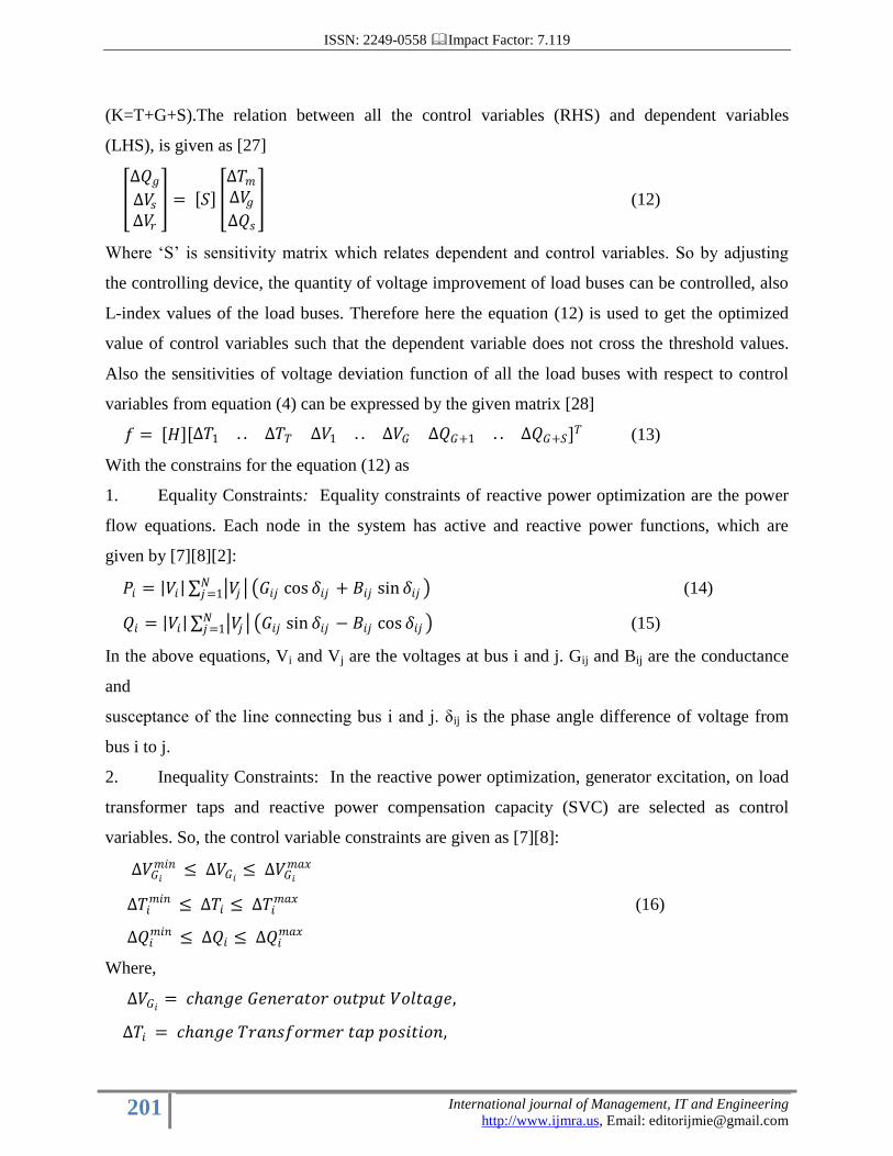
(K=T+G+S).The relation between all the control variables (RHS) and dependent variables

(LHS), is given as [27]

∆𝑄𝑔

∆𝑉𝑠∆𝑉𝑟

= 𝑆

∆𝑇𝑚∆𝑉𝑔∆𝑄𝑠

(12)

Where „S‟ is sensitivity matrix which relates dependent and control variables. So by adjusting

the controlling device, the quantity of voltage improvement of load buses can be controlled, also

L-index values of the load buses. Therefore here the equation (12) is used to get the optimized

value of control variables such that the dependent variable does not cross the threshold values.

Also the sensitivities of voltage deviation function of all the load buses with respect to control

variables from equation (4) can be expressed by the given matrix [28]

𝑓 = 𝐻 ∆𝑇1 . . ∆𝑇𝑇 ∆𝑉1 . . ∆𝑉𝐺 ∆𝑄𝐺+1 . . ∆𝑄𝐺+𝑆 𝑇 (13)

With the constrains for the equation (12) as

1. Equality Constraints: Equality constraints of reactive power optimization are the power

flow equations. Each node in the system has active and reactive power functions, which are

given by [7][8][2]:

𝑃𝑖 = 𝑉𝑖 𝑉𝑗 𝑁𝑗=1 𝐺𝑖𝑗 cos 𝛿𝑖𝑗 + 𝐵𝑖𝑗 sin 𝛿𝑖𝑗 (14)

𝑄𝑖 = 𝑉𝑖 𝑉𝑗 𝑁𝑗=1 𝐺𝑖𝑗 sin 𝛿𝑖𝑗 − 𝐵𝑖𝑗 cos 𝛿𝑖𝑗 (15)

In the above equations, Vi and Vj are the voltages at bus i and j. Gij and Bij are the conductance

and

susceptance of the line connecting bus i and j. δij is the phase angle difference of voltage from

bus i to j.

2. Inequality Constraints: In the reactive power optimization, generator excitation, on load

transformer taps and reactive power compensation capacity (SVC) are selected as control

variables. So, the control variable constraints are given as [7][8]:

∆𝑉𝐺𝑖

𝑚𝑖𝑛 ≤ ∆𝑉𝐺𝑖≤ ∆𝑉𝐺𝑖

𝑚𝑎𝑥

∆𝑇𝑖𝑚𝑖𝑛 ≤ ∆𝑇𝑖 ≤ ∆𝑇𝑖

𝑚𝑎𝑥 (16)

∆𝑄𝑖𝑚𝑖𝑛 ≤ ∆𝑄𝑖 ≤ ∆𝑄𝑖

𝑚𝑎𝑥

Where,

∆𝑉𝐺𝑖= 𝑐𝑕𝑎𝑛𝑔𝑒 𝐺𝑒𝑛𝑒𝑟𝑎𝑡𝑜𝑟 𝑜𝑢𝑡𝑝𝑢𝑡 𝑉𝑜𝑙𝑡𝑎𝑔𝑒,

∆𝑇𝑖 = 𝑐𝑕𝑎𝑛𝑔𝑒 𝑇𝑟𝑎𝑛𝑠𝑓𝑜𝑟𝑚𝑒𝑟 𝑡𝑎𝑝 𝑝𝑜𝑠𝑖𝑡𝑖𝑜𝑛,




∆𝑄𝑖 = 𝑐𝑕𝑎𝑛𝑔𝑒 𝑆𝑉𝐶 𝑠𝑒𝑡𝑡𝑖𝑛𝑔 𝑝𝑜𝑠𝑖𝑡𝑖𝑜𝑛𝑠,

∆𝑉𝐺𝑖

𝑚𝑖𝑛 = 𝑀𝑖𝑛𝑖𝑚𝑢𝑚 𝑜𝑢𝑡𝑝𝑢𝑡 𝑉𝑜𝑙𝑡𝑎𝑔𝑒 𝑜𝑓 𝐺𝑒𝑛𝑒𝑟𝑎𝑡𝑜𝑟,

∆𝑉𝐺𝑖

𝑚𝑎𝑥 = 𝑀𝑎𝑥𝑖𝑚𝑢𝑚 𝑜𝑢𝑡𝑝𝑢𝑡 𝑉𝑜𝑙𝑡𝑎𝑔𝑒 𝑜𝑓 𝐺𝑒𝑛𝑒𝑟𝑎𝑡𝑜𝑟,

∆𝑇𝑖𝑚𝑖𝑛 = 𝑀𝑖𝑛𝑖𝑚𝑢𝑚 𝑡𝑎𝑝 𝑝𝑜𝑠𝑖𝑡𝑖𝑜𝑛 𝑜𝑓 𝑇𝑟𝑎𝑛𝑠𝑓𝑜𝑟𝑚𝑒𝑟,

∆𝑇𝑖𝑚𝑎𝑥 = 𝑀𝑎𝑥𝑖𝑚𝑢𝑚 𝑡𝑎𝑝 𝑝𝑜𝑠𝑖𝑡𝑖𝑜𝑛 𝑜𝑓 𝑇𝑟𝑎𝑛𝑠𝑓𝑜𝑟𝑚𝑒𝑟,

∆𝑄𝑖𝑚𝑖𝑛 = 𝑀𝑖𝑛𝑖𝑚𝑢𝑚 𝑜𝑢𝑡𝑝𝑢𝑡 𝑜𝑓 𝑆𝑉𝐶’𝑠,

∆𝑄𝑖𝑚𝑎𝑥 = 𝑀𝑎𝑥𝑖𝑚𝑢𝑚 𝑜𝑢𝑡𝑝𝑢𝑡 𝑜𝑓 𝑆𝑉𝐶’𝑠.

The voltage of load bus and value of generator reactive power can be obtained after the

PF calculation. They are treated as state variables generally. The state variables constraints are

given by [1] [4] :

∆𝑉𝑖𝑚𝑖𝑛 ≤ ∆𝑉𝑖 ≤ ∆𝑉𝑖

𝑚𝑎𝑥

∆𝑄𝐺𝑖

𝑚𝑖𝑛 ≤ ∆𝑄𝐺𝑖≤ ∆𝑄𝐺𝑖

𝑚𝑎𝑥 (17)

∆𝑉𝑖𝑚𝑖𝑛 = 𝐿𝑜𝑤𝑒𝑟 𝑙𝑖𝑚𝑖𝑡 𝑜𝑓 𝑙𝑜𝑎𝑑 𝑣𝑜𝑙𝑡𝑎𝑔𝑒 𝑎𝑡 𝑎𝑛𝑦 𝑏𝑢𝑠 𝑖,

∆𝑉𝑖𝑚𝑎𝑥 = 𝑈𝑝𝑝𝑒𝑟 𝑙𝑖𝑚𝑖𝑡 𝑜𝑓 𝑙𝑜𝑎𝑑 𝑣𝑜𝑙𝑡𝑎𝑔𝑒 𝑎𝑡 𝑎𝑛𝑦 𝑏𝑢𝑠 𝑖,

∆𝑄𝐺𝑖

𝑚𝑖𝑛 = 𝐿𝑜𝑤𝑒𝑟 𝑙𝑖𝑚𝑖𝑡 𝑜𝑓 𝑔𝑒𝑛𝑒𝑟𝑎𝑡𝑜𝑟 𝑜𝑢𝑡𝑝𝑢𝑡 𝑜𝑓 𝑟𝑒𝑎𝑐𝑡𝑖𝑣𝑒 𝑝𝑜𝑤𝑒𝑟,

∆𝑄𝐺𝑖

𝑚𝑎𝑥 = 𝑈𝑝𝑝𝑒𝑟 𝑙𝑖𝑚𝑖𝑡 𝑜𝑓 𝑔𝑒𝑛𝑒𝑟𝑎𝑡𝑜𝑟 𝑜𝑢𝑡𝑝𝑢𝑡 𝑜𝑓 𝑟𝑒𝑎𝑐𝑡𝑖𝑣𝑒 𝑝𝑜𝑤𝑒𝑟,

∆𝑉𝑖 = 𝑐𝑕𝑎𝑛𝑔𝑒 𝐵𝑢𝑠 𝑉𝑜𝑙𝑡𝑎𝑔𝑒 𝑎𝑡 𝑎𝑛𝑦 𝑏𝑢𝑠 𝑖,

∆𝑄𝐺𝑖= 𝑅𝑒𝑎𝑐𝑡𝑖𝑣𝑒 𝑝𝑜𝑤𝑒𝑟 𝑔𝑒𝑛𝑒𝑟𝑎𝑡𝑖𝑜𝑛 𝑎𝑡 𝑎𝑛𝑦 𝑏𝑢𝑠 𝑖.

3. LP Technique

3.1 Approach for LP Technique in Power System

The flow chart of LP technique is shown in Flowchart 1[28]. Following are the steps

required [25]:

1. Read the system data for IEEE 39 bus system.

2. Increase the load demand and run the load flow analysis using fast decoupled load flow

method. Set the control variables at initial setting and calculate L-Index and system parameters at

each load bus using equation (5), (6) and (7).

3. Advance VAR control iteration count.

4. Calculate matrix S and H in equation (12) (13).

5. Apply LP Technique and calculate new control variable settings.




6. Check if control variables are in given threshold.

7. Perform Step 2 again with new settings of control variables.

8. If dependent variables obtained from equation (12), at each load bus are within their

constraints then stop otherwise go to step 3.

9. If there is significant change in objective function then go to step 3.

10. Calculate all system parameters, L-index and print result.

Flowchart 1. Flowchart of LP Technique Flowchart 2. Flowchart of PSO

Technique

4. Particle Swarm Optimization Algorithm

PSO is mathematically defined as [21][22]:

𝑌𝑖𝑗 𝑘 + 1 = 𝑊𝑌𝑖𝑗 𝑘 + 𝐶1𝑟1 𝑃𝑏𝑖𝑗 𝑘 − 𝑥𝑖𝑗 𝑘 + 𝐶2𝑟2(𝐺𝑏𝑖𝑗 𝑘 − 𝑥𝑖𝑗 𝑘 ) (18)




𝑥𝑖𝑗 𝑘 + 1 = 𝑥𝑖𝑗 𝑘 + 𝑌𝑖𝑗 𝑘 + 1 (19)

Where,

𝑊 is known as the weighting function.

𝑥𝑖𝑗 𝑘 = previous position of the particle.

𝑌𝑖𝑗 𝑘 = previous velocity of the particle.

𝑃𝑏 = best fitness of the particle so far.

𝐺𝑏 = best fitness of the swarm so far.

C1 = 2.1, C2 = 2, W = 0.5

4.1 Approach for PSO Technique in Power

System

The flowchart of PSO algorithm is shown in flowchart 2[28]. Following are the steps

required [6]:

1. Initialize parameter C1, C2 and W.

2. Give initial position and initial velocity for the particle of the swarm.

3. Calculate the fitness values of the particle. Calculate Pb and Gb.

4. Calculate the new velocity using equation(18)

5. Now update the position using (19)

6. Calculate the fitness values of the particle and update Pb and Gb.

7. If termination criteria are satisfied go to next step otherwise go to step 4.

8. Stop and print results.

5. Results and Analysis

MATPOWER is an open-source Matlab power system simulation package. It is used widely in

research and education for AC and DC power flow and optimal power flow (OPF) simulations.

MATPOWER consists of a set of Matlab M-files designed to give the best performance possible

while keeping the code simple to understand and customize. Matlab has become a popular tool

for scientific computing, combining a high-level language ideal for matrix and vector

computations, a cross-platform runtime with robust math libraries, an integrated development

environment and GUI with excellent visualization capabilities, and an active community of users

and developers. As a high-level scientific computing language, it is well suited for the numerical




computation typical of steady-state power system simulations. Owing to these advantages

MATPOWER is used in this project for the system calculation. The results obtained after

applying LP and PSO Techniques are shown in Table1, 2 and 3.

Table 1. 39 Bus System Controller Setting

The load flow analysis is done using fast decoupled load flow and load is increased by 30% in

the system. After the load is increased the initial voltages and losses in the buses are calculated

using load flow analysis. The values for the controller setting are obtained by applying

optimization Technique in suitable equations with given constraints. The Linear Programming

technique is applied using the mathematical model developed in the previous chapter. The

control variables are evaluated by LP technique and the variables are set in the system.

Thereafter system parameters are calculated. Similarly in Particle Swarm Optimization, the load

is increased by 30% in the system then control variables are randomly selected and PSO is

applied in the system. The control variables are selected for which the fitness function or

objective function is minimized. For the selected set of control variables, bus voltages, L-index

Controller Controller Settings

Initial LP PSO

V30 1.0000 1.0150 1.0129

V31 1.0000 1.0150 1.0344

V32 1.0000 1.0150 1.0130

V33 1.0000 1.0150 1.0073

V34 1.0000 1.0150 0.9841

V35 1.0000 1.0150 1.0195

V36 1.0000 1.0150 0.9978

V37 1.0000 1.0150 1.0319

V38 1.0000 1.0150 1.0132

V39 1.0000 1.0150 1.0411




and system parameters are calculated. The results of control variables obtained after applying

optimization techniques are shown in Table 1.

Bus

No.

Voltage Magnitudes (p.u.) L-Index values

Initial LP PSO Initial LP PSO

1 1.0011 1.0173 1.0364 0.0284 0.0272 0.0262

2 1.0038 1.0209 1.0274 0.0478 0.0456 0.0448

3 0.9824 1.0010 1.0064 0.0864 0.0821 0.0808

4 0.9510 0.9712 0.9795 0.1302 0.1233 0.1204

5 0.9556 0.9761 0.9880 0.1241 0.1170 0.1134

6 0.9602 0.9807 0.9928 0.1188 0.1119 0.1083

7 0.9447 0.9654 0.9787 0.1353 0.1277 0.1235

8 0.9436 0.9642 0.9779 0.1352 0.1276 0.1235

9 1.0008 1.0181 1.0392 0.0389 0.0366 0.0352

10 0.9834 1.0029 1.0096 0.0941 0.0889 0.0868

11 0.9739 0.9938 1.0024 0.1045 0.0986 0.0960

12 0.9542 0.9747 0.9825 0.1345 0.1273 0.1244

13 0.9758 0.9955 1.0022 0.1032 0.0976 0.0954

14 0.9651 0.9850 0.9910 0.1156 0.1095 0.1073

15 0.9658 0.9852 0.9856 0.1107 0.1052 0.1045

16 0.9873 1.0059 1.0040 0.0819 0.0779 0.0778

17 0.9886 1.0073 1.0080 0.0843 0.0802 0.0797

18 0.9848 1.0035 1.0060 0.0876 0.0834 0.0825

19 1.0321 1.0344 1.0383 0.0349 0.0339 0.0337

20 0.9658 0.9678 0.9721 0.0322 0.0321 0.0319

21 0.9827 0.9988 0.9991 0.0753 0.0717 0.0717

22 0.9977 1.0127 1.0133 0.0435 0.0414 0.0414

23 0.9903 1.0014 1.0023 0.0478 0.0459 0.0458

24 0.9914 1.0067 1.0073 0.0742 0.0705 0.0704

25 1.0168 1.0338 1.0422 0.0304 0.0287 0.0282

26 1.0112 1.0294 1.0324 0.0628 0.0597 0.0592

27 0.9945 1.0131 1.0151 0.0819 0.0779 0.0774

28 1.0146 1.0321 1.0327 0.0481 0.0457 0.0455

29 1.0168 1.0338 1.0336 0.0342 0.0324 0.0323




5.2 Results of Voltage and L-Index Values

. When the load is increased to 30% the output results acquired are shown in Table 2 in which

bus voltages and L-index for all buses are shown and compared with control variables for initial,

LP Technique and PSO algorithm. In the Table 2, the voltages V7, V8 and V12 are seen to be the

most critical load buses of the proposed 39 bus test power system. The proposed PSO algorithm

focuses more on nodes, in which voltage deviation are high. The model in this project suggests

measures to minimize voltage deviations. Thus improving the power system voltage profile and

hence voltage stability. After applying LP Technique significant changes in the voltages and L-

Index

values of the critical buses are observed. After applying PSO algorithm the results obtained are

compared with the initial and classical LP technique. From the table II, it is observed that the

minimum voltages enhances from an initial value of 0.9447 to 0.9654 in LP and to 0.9787 in

PSO algorithm for the bus 7. Similarly the voltage magnitude value increases from an initial

value of 0.9436 to 0.9642 in LP and to 0.9779 in PSO algorithm for the bus 8. Also for bus 12

the increment in voltage magnitude is observed as from initial value of 0.9542 to 0.9747 in LP

and to 0.9825 in PSO algorithm. The L-index value declines from an initial value of 0.1353 to

0.1277 in LP and to 0.1235 in PSO algorithm for the bus 7. Similarly the L-index value declines

from an initial value of 0.1352 to 0.1276 in LP and to 0.1235 in PSO algorithm for the bus 8.

Also for bus 12 the decline in L-index is observed as from initial value of 0.1345 to 0.1273 in LP

and to 0.1244 in PSO algorithm.

Table 2. 39-Bus System Voltage and L-index values at all selected load buses




5.3 Results of System Parameters For 39-Bus System

The system parameters are calculated after applying the control variables to the system. The

system parameters are basically the three objective functions which are to be minimized after the

increment of the load. In table III the system parameters calculation of the 39-bus system are

shown. From the Table 3, the voltage error Ve, voltage stability VL and power loss Ploss (MW)

are observed to reduce significantly after performing optimization algorithms. From the results

reported in Table 3, it is clearly observed that voltage deviation or voltage error Ve of the system

is reduced from initial value of 0.0221 to 0.0138 in LP and 0.0137 in PSO technique. Similarly,

the system power losses declines from initial value of 54.536MW to 52.466 MW in LP and to

52.029MW in PSO algorithm. The sum of squares of L-indices of system are reduced from

initial value of 0.2234 to 0.2003 in LP and to 0.1925 in PSO technique. Therefore from the

results we can conclude that the application of PSO technique to the system improves the voltage

profile as well as reduces losses of the system.

Table 3. 39 Bus System – System Parameters

5.4 Graphical Representation of Results

The graphical illustration of Table 2 only for critical buses is shown in Figure 1 and 2. The

improvement of voltage profile and their corresponding L-index values for critical buses are

shown in graph in Figure 1 and Figure 2.

Name of the

System

Parameter

System Parameters

Initial LP PSO

Ve 0.0221 0.0138 0.0138

VL 0.2234 0.2003 0.1925

Ploss(MW) 54.536 52.466 52.029




Figure 1. 39 bus system – Voltage profile Figure 2. 39- bus system – L-index values

for critical buses for critical load buses

Figure 3. 39 bus system – System Parameters

The value of voltage magnitudes for each critical bus is compared for different

optimization technique using the graphical representation Figure 1. Similarly, corresponding L-

index values for each critical load bus is compared graphically for every optimization algorithm

Figure 2. The graphical illustration of Table 3 is shown in Figure 3. The system parameters for

each optimization algorithm are also represented in graph for comparison in Figure 3. The graphs

of L-index and system parameters show a significant reduction in values after application of

optimization techniques. Also in the graph of voltage magnitude, there is observed a significant

enhancement in the values. This shows the effectiveness of the proposed algorithms for voltage

stability enhancement. The objective functions considered are reduced significantly and are

illustrated graphically in Figure 3.

0.115

0.12

0.125

0.13

0.135

0.14

V7 V8 V12

Initial

LP

PSO

0.92

0.93

0.94

0.95

0.96

0.97

0.98

0.99

V7 V8 V12

Initial

LP

PSO

0

0.2

0.4

0.6

Ve VL Ploss

Initial

LP

PSO




6. Conclusion

Voltage stability is plays an important role in the security of the power system. Analysis

of the system helps to prevent the voltage collapse and blackouts in the system. The proposed

method has been tested on MATLAB software and examined with different system parameters to

demonstrate its effectiveness and robustness. The indicator L-index is a quantitative measure for

the estimation of the distance of the actual state of the system to the stability limit. For a given

network, as the load/generation increases, the voltage magnitude and angles change, and for near

maximum power transfer condition, the voltage stability index Lj values for load buses tend to

close to 1, indicating that the system is close to voltage collapse. This feature of this indicator

has been exploited in our proposed algorithms to evolve a voltage collapse margin.

The PSO was developed to help the system to reach to optimum value at faster rate and thus

reducing the computational time. The results obtained from classical PSO are compared with

traditional Linear Programming optimization technique for an IEEE NEW ENGLAND 39-bus

system and it is verify that classical particle swarm optimization approach is effective in

reducing values of system parameters and hence improving the voltage stability of the system

than compared to Linear Programming technique.

REFERENCES

[1] K. Rayudu, G. Yesuratnam and A. Jayalaxmi, “Ant Colony Optimization Algorithm

Based Optimal Reactive Power Dispatch to Improve Voltage Stability”, 2017 International

Conference on circuits Power and Computing Technologies [ICCPCT].

[2] Kaushik Paul and Niranjan Kumar, “Application of MATPOWER for the Analysis of

Congestion in Power System Network and Determination of Generator Sensitivity Factor”,

International Journal of Applied Engineering Research ISSN 0973-4562 Volume 12, Number 6

(2017) pp.969-975.

[3] Sidnei do Nascimento and Maury M. Gouvêa Jr., “Voltage stability enhancement in

power systems with automatic facts device allocation”, 3rd International Conference on Energy

and Environment Research, ICEER 2016, 7-11 September 2016, Barcelona, Spain.




[4] K. Rayudu, G. Yesuratnam, K. Surendhar and A. Jayalaxmi, “Voltage Stability

Enhancement Based on Particle Swarm Optimization and LP Technique”, 2016 International

Conference on Emerging Technological Trends [ICETT].

[5] Tejaswini A. Gawande, Komal Kaur Khokhar, Tushar Sahare, Naveen Verma, Naved

Bakhtiyar and Dr. Altaf Badar, “Study of Different Methods of Voltage Stability Analysis”,

International Journal of Advanced Research in Electrical, Electronics and Instrumentation

Engineering, ISO 3297: 2007 Certified Organization, Vol. 4, Issue 11, November 2015.

[6] S. D. Chavan, Nisha P. Adgokar “An Overview on Particle Swarm Optimization: Basic

Concepts and Modified Variants”, International Journal of Science and Research Volume 4 Issue

5, May 2015. pp 255-260.

[7] Elfadil.Z. Yahia, Mustafa A. Elsherif, Mahmoud N. Zaggout, “Detection of Proximity to

Voltage Collapse by Using L –Index”, International Journal of Innovative Research in Science,

Engineering and Technology, An ISO 3297: 2007 Certified Organization Vol. 4, Issue 3, March

2015.

[8] Pathak Smita and Prof. B.N.Vaidya, “Optimal Power Flow by Particle Swarm

Optimization for Reactive Loss Minimization”, International Journal of Scientific & Technology

Research Volume 1, Issue 1,Feb 2012, ISSN 2277.8616.

[9] Ray Daniel Zimmerman, Member IEEE, Carlos Edmundo Murillo-Sánchez, Member

IEEE, and Robert John Thomas, Life Fellow IEEE, “MATPOWER: Steady-State Operations,

Planning, and Analysis Tools for Power Systems Research and Education”, IEEE

TRANSACTIONS ON POWER SYSTEMS, VOL. 26, NO. 1, FEBRUARY 2011.

[10] B. Singh, N. K. Sharma, and A. N. Tiwari. “Prevention of Voltage Instability by Using

FACTS Controllers in Power Systems: A Literature Survey,” International Journal of

Engineering Science and Technology, vol. 2, no. 5, pp. 980-992, 2010.

[11] Mudathir F. Akorede and Hashim Hizam, “Teaching Power System Analysis Course

using MATPOWER”, 2009 International Conference on Engineering Education (lCEED 2009),

December 7-8, 2009, Kuala Lumpur, Malaysia.

[12] J.K. Vis “Particle Swarm Optimizer for Finding Robust Optima”, 2009.

[13] K. Vaisakh, Member, IEEE, and P.Kanta Rao, “Optimum Reactive Power Dispatch

Using Differential Evolution for Improvement of Voltage Stability”, 978-1-4244-1762-9/08/ C

2008 IEEE.




[14] C. Reis and F. P M. Barbosa “A comparison of voltage stability indices,” IEEE-

MELECON, Benalmadena (Malaga), Spain, 2006.

[15] Dhadbanjan and Yesuratnam,“ Comparison of Optimum Reactive Power schedule with

Different Objectives using LP Technique”, Int. Journal of Emerging Electrical Power Systems,

Vol.7, no. 3, article.4, 2006, pp. 1-22.

[16] IEEE/CIGRE Joint Task Force on Stability Terms and Definitions, “Definition and

Classification of Power System Stability,” IEEE Transactions. on Power Systems, vol. 19, no.3,

pp. 1387-1401, 2004.

[17] M. A. Abido, “Optimal power flow using particle swarm optimization”, International

Journal of Electrical Power & Energy Systems, vol. 24, no.7, 2002, pp 563-571.

[18] Hirotaka Yoshida and Yoshikazu Fukuyama, member, IEEE, “A Particle Swarm

Optimization for Reactive Power and Voltage Control in Electric Power Systems Considering

Voltage Security Assessment”, 0-7803-5731-0A9y$10.000 1999 IEEE.

[19] CIGRE Task Force 38.02.14 Rep., “Analysis and modeling needs of power systems

under major frequency disturbances”, 1999.

[20] V. Ajjarapu, and C. Christy, “The continuation power flow A tool for steady state voltage

stability analysis,” IEEE Transactions on Power Systems, vol. 7, no. 1. pp. 416-423, 1992.

[21] J.Qiu and S.M.Shahidehpour, “A new approach for minimizing power losses and

improving voltage profile”, IEEE Trans. On Power Systems, vol. 2, no. 2, May 1987, pp. 287-

295.

[22] Kessel. P and Glavitsch. H, “Estimating the Voltage Stability of a Power System”, IEEE

Transactions on Power Delivery, vol.1, no.3, July 1986 pp. 346-354.

[23] K. R. C. Mamandur, Member, IEEE and R. D. Chenoweth, Senior Member, IEEE,

“Optimal Control Of Reactive Power Flow For Improvements In Voltage Profiles And For Real

Power Loss Minimization”, IEEE Transactions on Power Apparatus and Systems, Vol. PAS-

I1O, No. 7 July 1981.

[24] L. H. Fink and K. Carlsen, “Operating under stress and strain,” IEEE Spectrum, vol. 15,

no. 3, pp. 48-53, 1978.

[25] K. R. Padiyar, “Power System Dynamics Stability and Control”, Second edition by BS

Publications.

[26] P. Kundur, “Power System Stability and Control”, McGraw-Hill, Inc.




[27] Achille Messac, “Optimization in Practice with MATLAB For Engineering Students and

Professionals”, Cambridge University Press.

[28] Dhruvi Chopra and Prof. Y.D. Shahakar,” A Review on Augumentation of Voltage

Stability Using Optimization Technique”, IJRASET, vol 7, Issue 1, Jan 2019, pp 786-791.

a comparative study of optimization techniques for …

Documents