a comparative study of models for shear strength of ... · deep reinforced concrete beams are...
TRANSCRIPT

1
Abstract The shear behaviour of deep reinforced concrete beams has been a focus of experimental and analytical studies since the early 1950s, resulting in different approaches for predicting the shear strength of deep beams. This paper compares the main modelling assumptions of these approaches and summarizes the results from validation studies available in the literature. Based on these comparisons, a two-parameter kinematic theory (2PKT) and a mechanical model by Zararis are selected for further evaluation with the help of test series with different experimental variables. It is shown that both approaches predict the trends in beam series with varying shear-span-to-depth ratios, even though the mechanical model overestimates the shear strength of beams without web reinforcement. It is also shown that the two models differ significantly in capturing the effect of transverse reinforcement and the size effect in shear. While the 2PKT accounts for sliding shear failures which limit the effectiveness of transverse reinforcement beyond a certain reinforcement ratio, the mechanical model predicts a monotonic increase of shear strength with the ratio. The 2PKT is also shown to capture the size effect in shear observed in two series of tests well, while the mechanical model neglects this effect. Keywords: deep beams, shear capacity, prediction models, parametric study, size effect.
1 Introduction Deep reinforced concrete beams are characterized by small shear-span-to-depth ratios (a/d ≤ approx. 2.5), which makes them stiff structural members with high shear capacity. Owing to these characteristics deep beams are used as transfer girders in buildings, cap beams in bridge bents, pile caps in foundations, and other heavily loaded members. These members work predominantly in shear and develop complex deformation patterns which do not follow the classical plane-sections-
Paper 10 A Comparative Study of Models for Shear Strength of Reinforced Concrete Deep Beams J. Liu and B. Mihaylov Department of ArGEnCo, University of Liege, Belgium
Civil-Comp Press, 2015 Proceedings of the Fifteenth International Conference on Civil, Structural and Environmental Engineering Computing, J. Kruis, Y. Tsompanakis and B.H.V. Topping, (Editors), Civil-Comp Press, Stirlingshire, Scotland

2
remain-plane hypothesis for slender members. Clark conducted one of the earliest experimental studies on shear behaviour of deep beams in the early 1950s [1], followed by de Paiva and Siess [2], Leonhardt and Walther [3], Ramakrishnan and Ananthanarayana [4] in the 1960s. It was early recognized that instead of failing soon after the formation of diagonal cracks similarly to slender beams, deep beams could resist shear as much as 100% greater than that causing the critical diagonal crack [5]. Initially this extra capacity was considered unreliable, and the first formulas for the shear strength of deep beams were based on the load causing diagonal cracking. In the 1970s and early 1980s there was a return to an earlier concept for the shear design of beams, namely the truss analogy introduced by Ritter in 1899 and Mörsch in 1909. According to this analogy, a simply-supported deep beam subjected to a point load can be modelled as a truss consisting of two diagonal struts running from the load to the supports, and a horizontal tie representing the bottom flexural reinforcement. According to this simple strut-and-tie model, deep beams carry shear without significant tensile stresses in the web, and this explains the high shear capacity of such members. In 1984 the strut-and-tie models for deep beams and other concrete regions with complex deformation patterns were introduced for the first time in design code provisions in Canada [6]. In 1987 Schlaich et al. [7] generalized the strut-and-tie models as an approach which can form the basis for a consistent design of structural concrete. Since then researchers have proposed a number of strut-and-tie-models for deep beams, while others have developed different approaches in an attempt to better predict the shear capacity of members with small shear-span-to-depth ratios. This paper compares the modelling assumptions of different approaches for shear strength of deep beams, and focuses on a more detailed comparison of two mechanical models by using results from test series with different experimental variables.
2 Models for shear strength of deep beams 2.1 Categories of models Based on observations from experiments, a number of alternative approaches have been suggested by researchers to evaluate the shear strength of deep beams. As part of this study, models for deep beams from 73 articles published between 1987 and 2014 were reviewed and classified. These models were developed for beams under single curvature, typically subjected to three- or four- point bending. The models are divided into six main categories, namely strut-and-tie models, numerical models (i.e. finite element and discrete element models), artificial intelligence models, upper bound plasticity models, shear panel models, and other mechanical models. As can be seen from Figure 1, strut-and-tie models are the most frequently proposed by research studies, followed by numerical models and artificial intelligence models. The smallest category is other mechanical models, which includes a model proposed by Zararis [8] and a two-parameter kinematic theory (2PKT) by Mihaylov et al. [9].

3
Figure 1: Models for shear capacity of reinforced concrete deep beams published between 1987 and 2014.
Author(s) and year Category Type Size
effect
Validation results: Vexp/Vpred ratios
# of tests
Avg COV
Mau and Hsu, 1989 [10]
Shear-panel Semi-empirical No 63 1.00 8.2%
Wang et al., 1993 [11]
Upper-bound plasticity
Analytical No 64 1.02 12.5%
Aoyama, 1993 [12]
Strut-and-tie Analytical No 175 1.17 16.6%
Zielinski and Rigotti, 1995 [13]
Strut-and-tie Analytical No 24 1.20 24.6%
Ashour, 2000 [14]
Upper-bound plasticity
Analytical No 172 1.01 18.8%
Hwang et al., 2000 [15]
Strut-and-tie Analytical No 123 1.15 16.0%
Matamoros and Wang, 2003 [16]
Strut-and-tie Semi-empirical No 175 1.40 22.1%
Zararis, 2003 [8]
Other mechanical
Analytical No 145 1.01 10.5%
Tang and Tan, 2004 [17]
Strut-and-tie Analytical Yes 116 1.28 11.8%
Russo et al., 2004 [18]
Strut-and-tie Semi-empirical No 240 1.00 19.0%
Tang and Cheng, 2006 [19]
Strut-and-tie Analytical Yes 36 1.19 18.9%
Mihaylov et al., 2013 [9]
Other mechanical
Analytical Yes 434 1.10 13.7%
Table 1: Summary of models for shear strength of deep beams
Out of all reviewed approaches, Table 1 summarizes twelve models introduced between 1989 and 2013. Eleven of these models were selected from an earlier publication by Senturk and Higgins [20], and the list is completed by the more recent 2PKT approach. Out of the twelve models, seven are in the category of strut-
36%
30%
18%
8%
5%
3%Strut-and-tie models
Numerical models (FEM, DEM)
Artificial intelligence models
Upper-bound plasticity models
Shear panel models
Other mechanical models

4
and-tie models, two are upper bound plasticity models, one is shear panel model, and two are other mechanical models. Numerical models are excluded from the discussion because they are not developed specifically for deep beams and are significantly more complex than the rest of the approaches. Since one of the goals of this paper is to compare different physical assumptions for the modelling of deep beams, artificial intelligence models are also excluded from the discussion. As can be seen from Table 1, the selected models are also classified as either semi-empirical or analytical. By semi-empirical it is meant that the model is based on physical assumptions, and includes factors which are derived by fitting shear strengths obtained from deep beam tests. 2.2 Main model assumptions 2.2.1 Strut-and-tie models Strut-and-tie models are currently the most commonly used approach for the design of concrete regions with complex deformation patterns, including deep beams. This is evident from the fact that this approach is part of design code provisions such as ACI 318-08 [21], AASHTO LRFD [22], EC2 [23] among many others. In strut-and-tie models the flow of principal compression stresses in the concrete is represented by struts, the tension forces in the reinforcement are represented by ties, and the zones where the struts and ties join are modelled as nodal zoines under uniform stresses. All modern design provisions share these fundamentals, but differ mainly in terms of the stress limits for the struts and nodal zones, as well as in terms of limits on the angles between struts and ties. The codes provide a general framework for the use of strut-and-tie models, while the models listed in Table 1 are specifically developed for deep beams. Strut-and-tie models for deep beams can be either statically determinate or indeterminate, with the latter requiring estimation of the stiffness of the elements of the model. As this is a challenging problem, researchers often look for simple empirical relationships for the distribution of the forces among different mechanisms of shear resistance in deep beams.
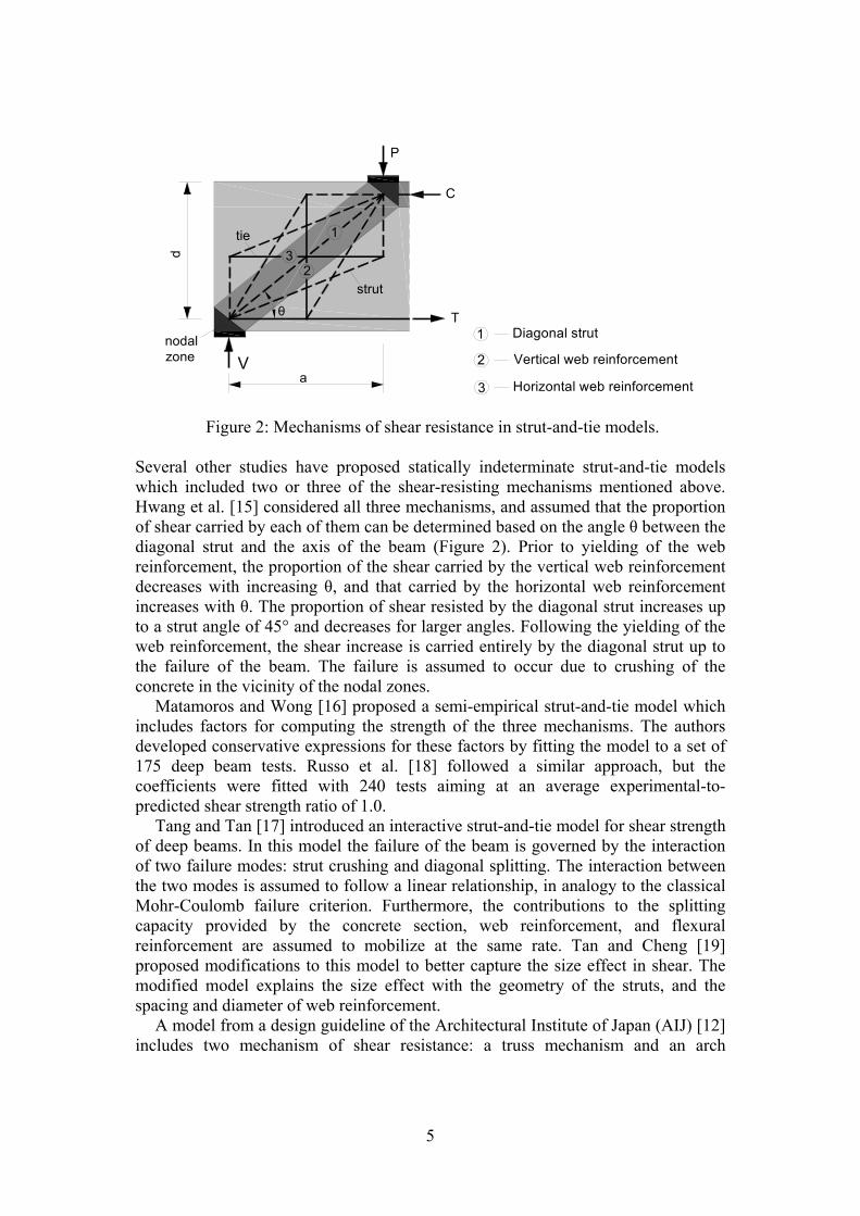
In the general case, strut-and-tie models for deep beams include three mechanisms of shear resistance: a direct diagonal strut between the load and the support, a truss mechanism involving the vertical web reinforcement, and a truss mechanism involving the horizontal web reinforcement, see Figure 2. The struts and ties join in two highly-stressed nodal zones in the vicinity of the loading and support points. Usually these mechanisms are taken into account explicitly in statically indeterminate models, while in statically determinate models the three mechanisms are merged and simplified.
Zielinski and Rigotti [13] proposed a statically determinate model for simply-supported deep beams with horizontal or inclined web reinforcement. They assumed a uniform field of struts in the web inclined at 45° with respect to the axis of the member. The ultimate shear capacity is govern by either strut crushing or yielding of the web reinforcement. According to this model, the maximum shear capacity occurs when the amount of web reinforcement is at least equal to that corresponding to balanced condition, where the capacity of the ties is equal to that of the struts.
5
Figure 2: Mechanisms of shear resistance in strut-and-tie models. Several other studies have proposed statically indeterminate strut-and-tie models which included two or three of the shear-resisting mechanisms mentioned above. Hwang et al. [15] considered all three mechanisms, and assumed that the proportion of shear carried by each of them can be determined based on the angle θ between the diagonal strut and the axis of the beam (Figure 2). Prior to yielding of the web reinforcement, the proportion of the shear carried by the vertical web reinforcement decreases with increasing θ, and that carried by the horizontal web reinforcement increases with θ. The proportion of shear resisted by the diagonal strut increases up to a strut angle of 45° and decreases for larger angles. Following the yielding of the web reinforcement, the shear increase is carried entirely by the diagonal strut up to the failure of the beam. The failure is assumed to occur due to crushing of the concrete in the vicinity of the nodal zones.
Matamoros and Wong [16] proposed a semi-empirical strut-and-tie model which includes factors for computing the strength of the three mechanisms. The authors developed conservative expressions for these factors by fitting the model to a set of 175 deep beam tests. Russo et al. [18] followed a similar approach, but the coefficients were fitted with 240 tests aiming at an average experimental-to-predicted shear strength ratio of 1.0.
Tang and Tan [17] introduced an interactive strut-and-tie model for shear strength of deep beams. In this model the failure of the beam is governed by the interaction of two failure modes: strut crushing and diagonal splitting. The interaction between the two modes is assumed to follow a linear relationship, in analogy to the classical Mohr-Coulomb failure criterion. Furthermore, the contributions to the splitting capacity provided by the concrete section, web reinforcement, and flexural reinforcement are assumed to mobilize at the same rate. Tan and Cheng [19] proposed modifications to this model to better capture the size effect in shear. The modified model explains the size effect with the geometry of the struts, and the spacing and diameter of web reinforcement.
A model from a design guideline of the Architectural Institute of Japan (AIJ) [12] includes two mechanism of shear resistance: a truss mechanism and an arch
nodalzone
d
aV
P
T
C
1
32
strut
tie
θ
1
2
3
Diagonal strut
Vertical web reinforcement
Horizontal web reinforcement

6
mechanism. Although this approach was not proposed as a strut-and-tie model, it is listed as such in Table 1 because of its similarity with some of the models discussed above. The truss mechanism consists of a uniform compression field in the web supported by the tension in the web reinforcement similarly to the model by Zielinski and Rigotti. The arch action on the other hand is similar to a direct diagonal strut running between the load and the support. The ultimate shear strength is attained when the web reinforcement is yielding and the diagonal web stresses reach the compressive strength of the concrete. The diagonal web stress is obtained by adding the average stress from the truss and arch mechanisms. The compressive strength of concrete is reduced by a factor which accounts for the effects of diagonal cracking in the web. The diagonal truss inclination is varied within a limited range of angles to maximize the shear strength. 2.2.2 Upper-bound plasticity models In upper-bound plasticity models deep beams are usually modelled as consisting of two rigid blocks separated by a yield line. The yield line typically represents the critical diagonal crack in the failing shear span of the beam. The concrete and steel are modelled as rigid - perfectly plastic materials, and the compressive strength of the concrete is reduced by an effectiveness factor to account for the real non-linear stress-strain behaviour of the material. The shear capacity of the beam is obtained by establishing a balance between the virtual work performed by the externally applied forces and that by the internal forces along the yield line, considering different directions of the displacements in the yield line. According to the upper-bound theorem of the theory of plasticity, the final solution corresponds to the lowest capacity obtained from these different failure mechanisms.
In the model by Wang et al. [11], the yield line is assumed straight and passes through the edge of the loading element in the critical shear span of the beam. The inclination of the yield line is varied together with the direction of the displacements in the line, in order to find the minimum failure load. The authors used a parabolic Coulomb-Mohr intrinsic curve as the yield criterion for the concrete. The model distinguishes between two cases of failure: failure with yielding of the vertical web reinforcement and failure with yielding of the horizontal reinforcement. An effectiveness factor for the concrete was proposed which is a function of the shear-span-to-depth ratio of the beam and equals 1.25-0.25(a/h).
In the model proposed by Ashour [14], the yield line extends from the inner edge of the support to the inner edge of the loading element, across the critical shear span of the beam. Two types of yield lines are proposed, namely a hyperbolic line and a line consisting of two straight segments. The failure criterion for the concrete in compression has a square shape in principal stress coordinate system, and the tensile strength is neglected. The shear capacity is expressed as a function of the position of the centre of relative rotation between the rigid blocks on each side of the yield line, and the solution of the model corresponds to the centre which produces a minimum shear capacity. The effectiveness factor for the concrete used in the model equals (0.8-fc/200), where fc is the compressive strength of the concrete in MPa.

7
2.2.3 Shear panel models Mau and Hsu have proposed a shear-panel model for deep beams [24] which was later adopted and modified by Bakir and Boduroǧlu [25], Yu and Hwang [26] and other researchers. In this model the web of the beam is modelled as a reinforced concrete panel subjected to uniform shear stresses v and effective transverse compressive stresses p. The transverse stresses are due to the direct action of the loads and support reactions on the horizontal top and bottom faces of the member. These stresses are sometimes referred to as clamping stresses, since they “clamp” the web in the vertical direction and increase its shear resistance. The ratio p/v is assumed to remain constant throughout the loading history, and is determined based on the shear-span-to-depth ratio a/h. As the a/h ratio increases, the p/v ratio decreases because the clamping stresses diminish away from point loads and support reactions. The shear strength of the panel, and therefore the shear strength of the beam, is obtained by solving simultaneous equations for equilibrium, compatibility of deformations, and constitutive relationships for the concrete and reinforcement. Since the solution of these equations is relatively complex and inconvenient for design, Mau and Hsu have proposed a simplified version of the model which is included in this study [10]. The original model was simplified by deriving a formula containing four constants, and these constants were obtained by a calibration with experimental data. 2.2.4 Other mechanical models In the mechanical model proposed by Zararis [8], the shear failure is assumed to occur along a critical diagonal crack with crushing of the concrete in the compression zone above this crack. As stated by the author, this zone acts as a “buffer” and prevents any meaningful slip displacements between the crack surfaces. In the absence of slip displacement, no aggregate interlock develops along the crack, and therefore the shear is carried entirely by the compression zone and the reinforcement crossing the crack. The resistance of the compression zone depends mainly on its depth above the critical crack, which can be significantly smaller than the depth of the compression zone above the flexural cracks. An expression is derived for the depth of the compression zone above the shear crack based on equilibrium conditions and several simplifying assumptions. According to this expression, the ratio between the depth above the shear crack and that above the flexural cracks depends on the shear-span-to-depth ratio and the ρv/ρl ratio, where ρv is the ratio of transverse reinforcement and ρl the ratio of bottom flexural reinforcement. The classical beam theory is used to evaluate the depth of the compression zone above the flexural cracks. The shear resistance is obtained by considering the horizontal and moment equilibrium of the part of the beam above the critical crack. At failure the stresses in the compression zone reach the compressive strength of the concrete, and the stresses in the transverse reinforcement are assumed equal to the yield strength of the steel. A similar approach is also followed to derive an expression for the shear strength of members with both transverse and horizontal web reinforcement.

8
The two-parameter kinematic theory (2PKT) [9] for shear behaviour of deep beams is built on a kinematic description of the deformation patterns in deep beams. Similarly to the models by Ashour and Zararis, the shear failure is assumed to occur along a critical diagonal crack which divides the shear span into two parts as shown in Figure 3a). The part below the crack is modelled by a fan of rigid radial struts while the zone above the crack is represented by a rigid block. The deformation pattern of the shear span is described by two degrees of freedom (DOFs): the average strain along the bottom reinforcement εt,avg and the vertical displacement in a critical loading zone (CLZ), Δc. The critical loading zone coincides with the compression zone above the critical diagonal crack discussed by Zararis. Degree of freedom εt,avg causes widening of the critical crack while c is associated with both widening and slip in the crack. In addition to the kinematic conditions, the 2PKT also includes equations for equilibrium and constitutive relationships for the mechanisms of shear resistance.
(a) Kinematics of deep beams
(b) Components of shear resistance and equilibrium at peak load
Figure 3: Two-parameter kinematic theory (2PKT) for deep beams.
Degree of freedom c is obtained by assuming that the CLZ is at failure under diagonal compressive stresses, while DOF εt,avg is obtained as illustrated in Figure 3b). The thick black line in the plot shows the relationship between εt,avg and the applied shear V, while the thick red line represents the shear resistance which
V
PcCLZ
d
x
z
h
1
a+ d cot t,avg
rigid block
fan
T
0
200
400
600
800
1000
1200
1400
1600
1800
0 0.5 1 1.5 2 2.5 3 3.5
She
ar F
orce
s, k
N
εt,avg, 10-3 (∆c = 2.13 mm)
VCLZ
Vs
Vci
Vd
V=ΣVi
V=T(0.9d)/a
equilibrium

9
decreases with increasing strains in the flexural reinforcement. This resistance consists of four components: shear carried in the CLZ, VCLZ, aggregate interlock component Vci, stirrups component Vs, and dowel action of the bottom reinforcement Vd. The solution of the equations of the 2PKT corresponds to the intersection point of the black and red lines where the shear forces are in equilibrium. This graphical representation of the 2PKT is similar to that used by Muttoni in a critical shear crack theory for punching of slabs [27]. With the predicted DOFs, the 2PKT can also be used to evaluate the deformation patterns of the beam near shear failure, including crack widths, deflections, and the complete displacement field of the beam.
3 Shear strength predictions Prediction results from the models discussed above are summarized in a chronological order in Figure 4 adapted from Senturk and Higgins [20]. The results are shown in terms of the shear strength experimental-to-predicted ratios Vexp/Vpred reported in the publications introducing the models. The centre of each vertical bar in the plot shows the average Vexp/Vpred ratio while the length of the bar corresponds to two standard deviations. The diameter of the bubbles represents the number of deep beam tests used for the validation of the models. The values plotted in Figure 4 are provided in the last three columns of Table 1. It can be seen that the average Vexp/Vpred varies from 1.00 to 1.40 and the coefficient of variation (COV) from 8.2% to 24.6%. It can also be seen that the number of tests used for the validation of the models varies greatly from 24 to 434.
Figure 4: Results from validation studies of models for shear strength of deep beams (adapted from Senturk and Higgins [20]).
If validated with the same experimental database, the shorter the vertical error bar and the closer its centre to the horizontal line at Vexp/Vpred = 1, the more accurate the model. On the other hand, the larger the experimental database (the bigger the
10 Russo et al., 2005
11 Tang and Cheng, 2006
12 Mihaylov, 2013
4 Zielinski and Rigotti, 1995
5 Ashour, 2000
6 Hwang et al, 2000
1 Mau and Hsu, 1989
2 Wang et al, 1993
3 Aoyama, 1993
7 Matamoros and Wang, 2003
8 Zararis, 2003
9 Tang and Tan, 2004

10
bubble), the more reliable the validation of the model. It can be seen from Figure 4 that while some models produced more accurate results than others, they were validated with a relatively small number of tests. It is therefore of interest to compare in more detail the most extensively validated model, i.e. the 2PKT approach, with a model which produced a lower coefficient of variation (COV) for a relatively large database of tests. Among the models which produced smaller COV than the 2PKT approach, the mechanical model by Zararis has been validated with the largest number of tests. Furthermore, this model has been highlighted by Senturk and Higgins in their study on analytical methods for deck girder bridge bent caps [20] as a modal which stands out in the literature due to the absence of empirical expressions. The model by Zararis has been validated with 145 tests producing a coefficient of variation of 10.5% compared to 434 tests and a COV of 13.7% for the 2PKT approach. The average shear strength experimental-to-predicted ratios for the two models are respectively 1.01 and 1.10.
4 Comparisons with test series In the following sections the 2PKT approach and the mechanical model by Zararis will be evaluated in terms of their ability to capture the effect of different experimental variables on the shear strength of individual series of deep beam specimens. The experimental variables include the shear-span-depth-ratio a/d, the ratio of flexural reinforcement ρl, the ratio of transverse web reinforcement ρv, and the size of the member (size effect in shear).
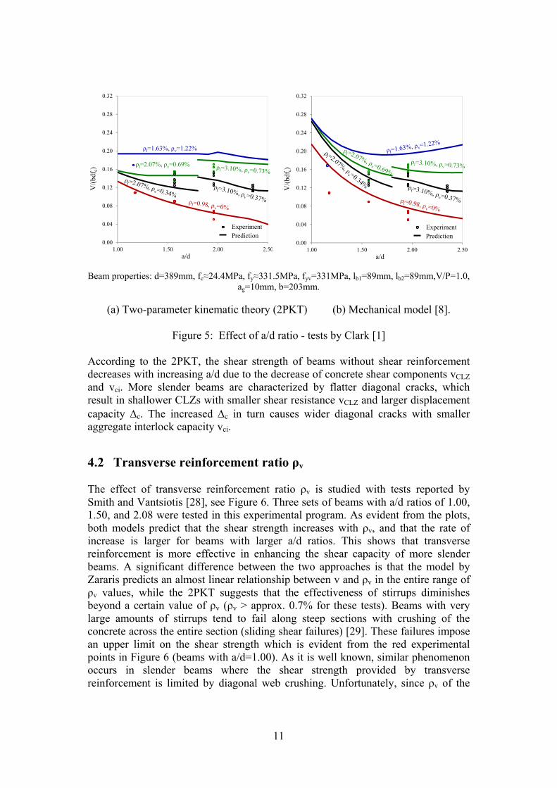
4.1 Effect of shear-span-to-depth-ratio a/d Figure 5 shows the effect of the a/d ratio on the shear strength of deep beams tested by Clark [1]. This effect is studied for four series of beams with different reinforcement ratios l from 0.98% to 3.05% and v from 0 to 1.22%. The experimentally obtained shear strengths are indicated with circles, while the predictions of the 2PKT approach and the model by Zararis are depicted with continuous lines. Both models predict that the shear strength decreases with increasing a/d from 1.0 to 2.5, and that the rate of decrease is reduced by the addition of transverse reinforcement. Exception is the case of beams with maximum transverse reinforcement for which the model by Zararis predicts that the shear strength increases when a/d exceeds about 1.7. The discontinuity in the black and green lines in the plots show that increased amounts of flexural reinforcement l results in increased shear strength predictions. These trends match the trends indicated by the experimental data, even though the two models differ in terms of the absolute values of the predicted shear strengths. It can be seen that the model by Zararis produces unconservative predictions for the specimens without web reinforcement (red line), while the 2PKT captures mostly the average experimental values. The shear strength of the only specimen with maximum amount of transverse reinforcement (v=1.22%) is overestimated by both models.
11
Beam properties: d=389mm, fc≈24.4MPa, fy≈331.5MPa, fyv=331MPa, lb1=89mm, lb2=89mm,V/P=1.0, ag=10mm, b=203mm.
(a) Two-parameter kinematic theory (2PKT) (b) Mechanical model [8].
Figure 5: Effect of a/d ratio - tests by Clark [1]
According to the 2PKT, the shear strength of beams without shear reinforcement decreases with increasing a/d due to the decrease of concrete shear components vCLZ and vci. More slender beams are characterized by flatter diagonal cracks, which result in shallower CLZs with smaller shear resistance vCLZ and larger displacement capacity c. The increased c in turn causes wider diagonal cracks with smaller aggregate interlock capacity vci.
4.2 Transverse reinforcement ratio ρv The effect of transverse reinforcement ratio ρv is studied with tests reported by Smith and Vantsiotis [28], see Figure 6. Three sets of beams with a/d ratios of 1.00, 1.50, and 2.08 were tested in this experimental program. As evident from the plots, both models predict that the shear strength increases with ρv, and that the rate of increase is larger for beams with larger a/d ratios. This shows that transverse reinforcement is more effective in enhancing the shear capacity of more slender beams. A significant difference between the two approaches is that the model by Zararis predicts an almost linear relationship between v and ρv in the entire range of ρv values, while the 2PKT suggests that the effectiveness of stirrups diminishes beyond a certain value of ρv (ρv > approx. 0.7% for these tests). Beams with very large amounts of stirrups tend to fail along steep sections with crushing of the concrete across the entire section (sliding shear failures) [29]. These failures impose an upper limit on the shear strength which is evident from the red experimental points in Figure 6 (beams with a/d=1.00). As it is well known, similar phenomenon occurs in slender beams where the shear strength provided by transverse reinforcement is limited by diagonal web crushing. Unfortunately, since ρv of the
0.00
0.04
0.08
0.12
0.16
0.20
0.24
0.28
0.32
1.00 1.50 2.00 2.50
V/(
bdf c
)
a/d
ρl=2.07%, ρv=0.69%
ρl=1.63%, ρv=1.22%
PredictionExperiment
0.00
0.04
0.08
0.12
0.16
0.20
0.24
0.28
0.32
1.00 1.50 2.00 2.50
V/(
bdf c
)
a/d
PredictionExperiment

12
specimens with a/d of 1.50 and 2.08 did not exceed 0.77%, these test series cannot be used to draw a stronger conclusion on the maximum shear strength of deep beams.
Beam properties: d=305mm, fc≈20MPa, ρl=1.94%, fy=422MPa, fyv=460MPa, lb1=102mm, lb2=102mm, V/P=1, ag=13mm, b=102mm.
(a) Two-parameter kinematic theory (2PKT) (b) Mechanical model [8]
Figure 6: Effect of transverse reinforcement ratio- tests by Smith and Vantsiotis [28]
4.3 Size effect in shear The size effect in deep beams was investigated by Zhang and Tan [30] who tested two series of geometrically similar beams with variable depth of the section, see Figure 7. The experimental points in the plot show that when the effective depth of the section was increased from 313 mm to 904 mm, the shear stress at failure decreased by 18.1% and 13.9% for beams with and without stirrups, respectively. This size effect in shear can be important, since the depth of deep beams in buildings and bridges can be significantly larger than 904 mm, often reaching 3 to 6 m. As indicated in Table 1, three of the twelve models discussed in this study account for the size effect in shear. The prediction lines in Figure 7a) show that the 2PKT approach captures well the decrease in shear strength observed in the tests. The model explains this decrease mainly with the weakening of the aggregate interlock mechanism. Larger beams have bigger critical loading zones with larger
displacement capacities c. As discussed earlier, larger c result in wider diagonal cracks and diminishing shear stresses transferred across the cracks. The 2PKT predicts that beams with transverse reinforcement will exhibit a slightly smaller size effect mainly due to the smaller proportion of shear resistance provided by the
0.00
0.05
0.10
0.15
0.20
0.25
0.30
0.35
0.0 0.2 0.4 0.6 0.8 1.0 1.2 1.4
V/(
bdf c
)
ρv (%)
a/d=1.00
Prediction
Experiment
0.00
0.05
0.10
0.15
0.20
0.25
0.30
0.35
0.0 0.2 0.4 0.6 0.8 1.0 1.2 1.4
V/(
bdf c
)
ρv (%)
Prediction
Experiment

13
aggregate interlock. As evident from Figure 7b), the mechanical model by Zararis neglects the size effect in deep beams.
Beam properties: a/d=1.1, h=1.075d, fc≈28.1MPa, ρl=1.26%, fy≈495 MPa, lb1=0.16d, lb2=0.16d, V/P=1, ag=10mm, b=0.25d.
(a) Two-parameter kinematic theory (2PKT) (b) Mechanical model [8].
Figure 7: Size effect in shear – tests by Zhang and Tan [30]
4.4 Summary of results The results from the test series discussed above are summarized in an appendix to this paper. The table contains the geometrical and material properties of the 72 specimens, as well as the experimentally obtained shear strengths Vexp. These strengths are compared with the predictions produced by the 2PKT approach and the mechanical model by Zararis in terms of shear strength experimental-to-predicted ratios Vexp/Vpred. The 2PKT produced an average Vexp/Vpred ratio of 1.06 with a coefficient of variation (COV) of 12.7% compared to 0.97 and 20.8% produced by the mechanical model.
5 Concluding remarks As part of this study, models for shear strength of deep beams from 73 articles published between 1987 and 2014 were reviewed. The models were divided into six categories based on their main features: strut-and-tie models, upper-bound plasticity models, shear panel models, other mechanical models, artificial intelligence models, and numerical models. Twelve models from the first four categories were selected based on an earlier study by Senturk and Higgins [20] and more recent developments. The main assumptions of these models were summarized, and the prediction results reported by the authors of the models were compared. It was
0.00
0.05
0.10
0.15
0.20
0.25
100 1000
V/(
bdf c
)
h, mm
ρvfyv=1.75MPa
ρvfyv=0
Experiment
Prediction
30000.00
0.05
0.10
0.15
0.20
0.25
100 1000V
/(bd
f c)
h, mm
ρvfyv=1.75MPa
ρvfyv=0
Experiment
Prediction
3000

14
shown that the average shear strength experimental-to-predicted ratios Vexp/Vpred varied from 1.00 to 1.40 for the different approaches, and the coefficients of variation (COV) varied from 8.2% to 24.6%. It was also shown that the number of tests used for the validation of the models varied greatly between 24 and 434.
Two models were selected for further comparisons: a two-parameter kinematic theory (2PKT) [9] and a mechanical model by Zararis [8]. The former was validated with the largest number of tests, while the latter produced a smaller COV than the kinematic approach for a relatively large number of tests. The models were compared in terms of their ability to capture the effect of different experimental variables on the shear strength of deep beams. It was shown that both models capture well the trends in tests with variable a/d ratios, even though the model by Zararis produced unconservative predictions for beams without web reinforcement. It was also found that the two models differ significantly in predicting the effect of transverse reinforcement ratio ρv. While the mechanical model predicts an almost linear increase of shear strength with ρv, the 2PKT accounts for sliding shear failures which impose an upper limit on the shear capacity of beams with large amounts of stirrups. The two models also differ in capturing the size effect in shear. The 2PKT captured well this effect observed in two series of deep beam tests, while the mechanical model neglects the size effect. Finally, it is noted that the 2PKT approach can be used to predict both shear strength and deformation patterns near failure, while the rest of the approaches discussed in this study were developed specifically for shear strength calculations.
References [1] A.P. Clark, “Diagonal tension in reinforced concrete beams,” ACI Structural
Journal, 48(10), 145-56, 1951. [2] H.A.R. de Paiva and C.P. Siess, “Strength and behaviour of deep beams in
shear,” Journal of Structural Engineering, 91(5), 19-41, 1965. [3] F. Leonhardt and R. Walther, “Wandartige trager,” Deutscher Ausschuss für
Stahlbeton, Berlin, 178, 1966. [4] V. Ramakrishnan and Y. Ananthanarayana, “Ultimate strength of deep beams
in shear,” ACI Journal Proceedings, 65(2), 87-98 1968. [5] ACI-ASCE Committee 326, “Shear and diagonal tension,” ACI Structural
Journal, Vol. 59, No. 1, 2, and 3, Jan., Feb., and Mar. 1962, pp. 1-30, 277-334, and 352-1349; also discussion and closure, Vol. 59, No. 10, Oct. 1962, pp. 1323-1349.
[6] M.P. Collins and D. Mitchell, “A rational approach to shear design – the 1984 Canadian code provisions,” ACI Structural Journal, 83(6), 925-933, 1986.
[7] J. Schlaich, K. Schafer and M. Jennewein, “Towards a consistent design of structural concrete,” PCI Journal, 32 (3), 74-150, 1987.
[8] P.D. Zararis, “Shear compression failure in reinforced concrete deep beams,” Journal of Structural Engineering, 129(4), 544-53, 2003.
[9] B.I. Mihaylov, E.C. Bentz and M.P. Collins, “Two-parameter kinematic theory for shear behaviour of deep beams,” ACI Structural Journal, 110 (3), 447-56, 2013.

15
[10] S.T. Mau, T.T.C. Hsu, “Formula for the shear strength of deep beams,” ACI Structural Journal, 86(5), 516-23, 1989.
[11] W. Wang, D. Jiang, and T. T. C Hsu, “Shear strength of reinforced concrete deep beams,” Journal of Structural Engineering, 119(8), 2294-2312, 1993.
[12] H. Aoyama, “Design philosophy for shear in earthquake resistance in Japan,” Earthquake Resistance of Reinforced Concrete Structures-A Volume Honoring Hiroyuki Aoyama, University of Tokyo Press, Tokyo, Japan, 407-418, 1993
[13] Z. A. Zielinski, and M. Rigotti, “Tests on shear capacity of reinforced concrete,” Journal of Structural Engineering, 121(11), 1660-1666, 1995.
[14] A.F. Ashour, “Shear capacity of reinforced concrete deep beams,” Journal of Structural Engineering, 126(9), 1045-52, 2000.
[15] S.J. Hwang, W.Y. Lu, H.J. Lee, “Shear strength prediction for deep beams,” ACI Structural Journal, 97(3), 367-76, 2000.
[16] A.B. Matamoros, K.H. Wong, “Design of simply supported deep beams using strut-and-tie models,” ACI Structural Journal, 100(6), 704-12, 2003.
[17] C.Y. Tang, K.H. Tan, “Interactive mechanical model for shear strength of deep beams,” Journal of Structural Engineering, 130(10), 1534-44, 2004.
[18] G. Russo, R. Venir and M. Pauletta, “Reinforced concrete deep beams shear strength model and design formula,” ACI Structural Journal, 102(3), 429-37, 2005.
[19] K.H. Tan and G.H. Cheng, “Size effect on shear strength of deep beams: investigating with strut-and-tie model,” Journal of Structural Engineering, 132(5), 673-85, 2006.
[20] A.E. Senturk, C. Higgins, “Evaluation of reinforced concrete deck girder bridge bent caps with 1950s vintage details: analytical methods,” ACI Structural Journal, 107(5), 544-553, 2010.
[21] ACI Committee 318, “Building code requirements for dtructural voncrete (ACI 318-08) and vommentary,” American Concrete Institute, Farmington Hills, MI, 2008.
[22] AASHTO, “AASHTO LRFD bridge design specifications, fourth edition,” American Association of State highway officials, Washington, DC, 2007.
[23] European Committee for Standardization, “EN 1992-1-1 Eurocode 2: Design of concrete structures – Part 1-1: General rules and rules for buildings,” CEN, Brussels, 2004.
[24] S.T. Mau and C.-T.T. Hsu, “Shear strength prediction for deep beams with web reinforcement,” ACI Structural Journal, 84(6), 513-23, 1987.
[25] P.G. Bakir and H.M. Boduroǧlu, “Mechanical behaviour and non-linear analysis of short beams using softened truss and direct strut & tie models,” Engineering Structures, 27(4), 639-51, 2005.
[26] H.W. Yu and S.J. Hwang, “Evaluation of softened truss model for strength prediction of reinforced concrete squat walls,” Journal of Engineering Mechanics, 131(8), 839-46, 2005.
[27] A. Muttoni, “Punching shear strength of reinforced concrete slabs without transverse reinforcement,” ACI Structural Journal, 105(4), 440-450, 2008.
[28] K.N. Smith and A.S. Vantsiotis, “Shear strength of deep beams,” ACI Structural Journal, 79(3), 201-13, 1982.

16
[29] D. Lee, “An experimental investigation in the effects of detailing on the shear behaviour of deep beams,” Master Thesis, Department of Civil Engineering, University of Toronto, 1982.
[30] N. Zhang and K.H. Tan, “Size effect in RC deep beams: Experimental Investigation and STM Verification,” Engineering Structures, 29(12), 3241-54, 2007.
Symbols a = shear span ag = maximum size of coarse aggregate b = width of section d = effective depth of section fc = concrete cylinder strength fy = yield strength of bottom longitudinal bars fyv = yield strength of stirrups h = total depth of section lb1 = width of loading element parallel to longitudinal axis of member lb2 = width of support parallel to longitudinal axis of member P = applied concentrated load T = tension force in bottom reinforcement V = shear force Vc = shear resisted by diagonal strut Vexp = experimentally obtained shear strength Vpred = predicted shear strength VCLZ = shear resisted by the CLZ Vci = shear resisted by aggregate interlock Vd = shear resisted by dowel action Vs = shear resisted by stirrups θ = angle of diagonal strut
c = transverse displacement capacity of critical loading zone
εt,avg = average strain along bottom longitudinal reinforcement ρh = ratio of horizontal web reinforcement ρl = ratio of tensile longitudinal reinforcement ρv = ratio of transverse reinforcement

17
Ap
pen
dix
Ref
. #
Bea
m
Nam
e a/
d b
(m
m)
d
(mm
) h
(mm
)a
(m
m)
l b1
(m
m)
l b2
(m
m)
V/P
ρ
l1
(%)
# b
ars1
f y1
(M
pa)
ag
(mm
) f c
(M
pa)
ρv
(%)
d bv
(mm
)f y
v (M
Pa)
ρh
(%)
f yh
(MP
a)V
exp
(kN
) 2P
KT
E
xp/P
red
Zar
aris
E
xp/P
red
[1]
D
0-1
1.17
20
3 38
9 45
7 45
7 89
89
1
0.98
2
370
10
25.9
0
0
0
221.
6 0.
96
0.66
D0-
3 1.
17
203
389
457
457
89
89
1 0.
98
2 37
0 10
26
.0
0
0 0
22
3.2
0.96
0.
66
C0-
1 1.
57
203
389
457
610
89
89
1 0.
98
2 37
0 10
24
.7
0
0 0
17
4.3
1.06
0.
84
C0-
3 1.
57
203
389
457
610
89
89
1 0.
98
2 37
0 10
23
.6
0
0 0
16
6.9
1.05
0.
83
B0-
1 1.
96
203
389
457
762
89
89
1 0.
98
2 37
0 10
23
.6
0
0 0
12
1.0
0.99
0.
84
B0-
2 1.
96
203
389
457
762
89
89
1 0.
98
2 37
0 10
23
.9
0
0 0
94
.2
0.77
0.
65
B0-
3 1.
96
203
389
457
762
89
89
1 0.
98
2 37
0 10
23
.5
0
0 0
12
8.0
1.05
0.
90
C1-
1 1.
57
203
389
457
610
89
89
1 2.
07
2 32
1 10
25
.6
0.34
9.
5 33
1 0
27
7.7
1.13
0.
96
C1-
2 1.
57
203
389
457
610
89
89
1 2.
07
2 32
1 10
26
.3
0.34
9.
5 33
1 0
31
1.1
1.25
1.
05
C1-
3 1.
57
203
389
457
610
89
89
1 2.
07
2 32
1 10
24
.0
0.34
9.
5 33
1 0
24
5.9
1.03
0.
88
C1-
4 1.
57
203
389
457
610
89
89
1 2.
07
2 32
1 10
29
.0
0.34
9.
5 33
1 0
28
5.9
1.10
0.
91
B1-
1 1.
96
203
389
457
762
89
89
1 3.
10
3 32
1 10
23
.4
0.37
9.
5 33
1 0
27
8.8
1.08
1.
15
B1-
2 1.
96
203
389
457
762
89
89
1 3.
10
3 32
1 10
25
.4
0.37
9.
5 33
1 0
25
6.6
0.97
1.
01
B1-
3 1.
96
203
389
457
762
89
89
1 3.
10
3 32
1 10
23
.7
0.37
9.
5 33
1 0
28
4.8
1.10
1.
17
B1-
4 1.
96
203
389
457
762
89
89
1 3.
10
3 32
1 10
23
.3
0.37
9.
5 33
1 0
26
8.1
1.04
1.
11
B1-
5 1.
96
203
389
457
762
89
89
1 3.
10
3 32
1 10
24
.6
0.37
9.
5 33
1 0
24
1.4
0.92
0.
97
A1-
1 2.
35
203
389
457
914
89
89
0.5
3.10
3
321
10
24.6
0.
38
9.5
331
0
222.
5 0.
95
1.01
A1-
2 2.
35
203
389
457
914
89
89
0.5
3.10
3
321
10
23.6
0.
38
9.5
331
0
209.
1 0.
91
0.97
A1-
3 2.
35
203
389
457
914
89
89
0.5
3.10
3
321
10
23.4
0.
38
9.5
331
0
222.
5 0.
97
1.03
A1-
4 2.
35
203
389
457
914
89
89
0.5
3.10
3
321
10
24.8
0.
38
9.5
331
0
244.
7 1.
05
1.10
C2-
1 1.
57
203
389
457
610
89
89
1 2.
07
2 32
1 10
23
.6
0.69
9.
5 33
1 0
28
9.9
1.00
0.
94
C2-
2 1.
57
203
389
457
610
89
89
1 2.
07
2 32
1 10
25
.0
0.69
9.
5 33
1 0
30
1.1
1.04
0.
95
C2-
4 1.
57
203
389
457
610
89
89
1 2.
07
2 32
1 10
27
.0
0.69
9.
5 33
1 0
28
8.1
0.98
0.
87
D4-
1 1.
16
203
395
457
457
89
89
1 1.
63
2 33
5 10
23
.1
1.22
9.
5 33
1 0
31
2.2
0.87
0.
73
[28
] 0A
0-44
1.
00
102
305
356
305
102
102
1 1.
94
3 42
2 12
.7
20.5
0
0
139.
5 1.
02
0.79
0A0-
48
1.00
10
2 30
5 35
6 30
5 10
2 10
2 1
1.94
3
422
12.7
20
.9
0
0
13
6.1
0.98
0.
76

18
Ref
. #
Bea
m
Nam
e a/
d b
(m
m)
d
(mm
) h
(mm
)a
(m
m)
l b1
(m
m)
l b2
(m
m)
V/P
ρ
l1
(%)
# b
ars1
f y1
(M
pa)
ag
(mm
) f c
(M
pa)
ρv
(%)
d bv
(mm
)f y
v (M
Pa)
ρh
(%)
f yh
(MP
a)V
exp
(kN
) 2P
KT
E
xp/P
red
Zar
aris
E
xp/P
red
1A1-
10
1.00
10
2 30
5 35
6 30
5 10
2 10
2 1
1.94
3
422
12.7
18
.7
0.28
6.
4 46
0 0.
23
460
161.
2 1.
21
0.97
1A2-
11
1.00
10
2 30
5 35
6 30
5 10
2 10
2 1
1.94
3
422
12.7
18
.0
0.28
6.
4 46
0 0.
45
460
148.
3 1.
13
0.92
1A3-
12
1.00
10
2 30
5 35
6 30
5 10
2 10
2 1
1.94
3
422
12.7
16
.1
0.28
6.
4 46
0 0.
68
460
141.
2 1.
16
0.96
1A4-
51
1.00
10
2 30
5 35
6 30
5 10
2 10
2 1
1.94
3
422
12.7
20
.5
0.28
6.
4 46
0 0.
68
460
170.
9 1.
21
0.97
1A6-
37
1.00
10
2 30
5 35
6 30
5 10
2 10
2 1
1.94
3
422
12.7
21
.1
0.28
6.
4 46
0 0.
91
460
184.
1 1.
28
1.03
2A1-
38
1.00
10
2 30
5 35
6 30
5 10
2 10
2 1
1.94
3
422
12.7
21
.7
0.63
6.
4 46
0 0.
23
460
174.
5 1.
18
0.91
2A3-
39
1.00
10
2 30
5 35
6 30
5 10
2 10
2 1
1.94
3
422
12.7
19
.8
0.63
6.
4 46
0 0.
45
460
170.
6 1.
22
0.96
2A4-
40
1.00
10
2 30
5 35
6 30
5 10
2 10
2 1
1.94
3
422
12.7
20
.3
0.63
6.
4 46
0 0.
68
460
171.
9 1.
21
0.95
2A6-
41
1.00
10
2 30
5 35
6 30
5 10
2 10
2 1
1.94
3
422
12.7
19
.1
0.63
6.
4 46
0 0.
91
460
161.
9 1.
18
0.94
3A1-
42
1.00
10
2 30
5 35
6 30
5 10
2 10
2 1
1.94
3
422
12.7
18
.4
1.25
6.
4 46
0 0.
23
460
161.
0 1.
20
0.87
3A3-
43
1.00
10
2 30
5 35
6 30
5 10
2 10
2 1
1.94
3
422
12.7
19
.2
1.25
6.
4 46
0 0.
45
460
172.
7 1.
25
0.92
3A4-
45
1.00
10
2 30
5 35
6 30
5 10
2 10
2 1
1.94
3
422
12.7
20
.8
1.25
6.
4 46
0 0.
68
460
178.
6 1.
23
0.91
3A6-
46
1.00
10
2 30
5 35
6 30
5 10
2 10
2 1
1.94
3
422
12.7
19
.9
1.25
6.
4 46
0 0.
91
460
168.
1 1.
19
0.89
0C0-
50
1.50
10
2 30
5 35
6 45
7 10
2 10
2 1
1.94
3
422
12.7
20
.7
0
0
11
5.7
1.23
1.
20
1C1-
14
1.50
10
2 30
5 35
6 45
7 10
2 10
2 1
1.94
3
422
12.7
19
.2
0.18
6.
4 46
0 0.
23
460
119.
0 1.
15
1.24
1C3-
02
1.50
10
2 30
5 35
6 45
7 10
2 10
2 1
1.94
3
422
12.7
21
.9
0.18
6.
4 46
0 0.
45
460
123.
4 1.
11
1.20
1C4-
15
1.50
10
2 30
5 35
6 45
7 10
2 10
2 1
1.94
3
422
12.7
22
.7
0.18
6.
4 46
0 0.
68
460
131.
0 1.
16
1.26
1C6-
16
1.50
10
2 30
5 35
6 45
7 10
2 10
2 1
1.94
3
422
12.7
21
.8
0.18
6.
4 46
0 0.
91
460
122.
3 1.
11
1.22
2C1-
17
1.50
10
2 30
5 35
6 45
7 10
2 10
2 1
1.94
3
422
12.7
19
.9
0.31
6.
4 46
0 0.
23
460
124.
1 1.
10
1.20
2C3-
03
1.50
10
2 30
5 35
6 45
7 10
2 10
2 1
1.94
3
422
12.7
19
.2
0.31
6.
4 46
0 0.
45
460
103.
6 0.
93
1.04
2C3-
27
1.50
10
2 30
5 35
6 45
7 10
2 10
2 1
1.94
3
422
12.7
19
.3
0.31
6.
4 46
0 0.
45
460
115.
3 1.
03
1.15
2C4-
18
1.50
10
2 30
5 35
6 45
7 10
2 10
2 1
1.94
3
422
12.7
20
.4
0.31
6.
4 46
0 0.
68
460
124.
6 1.
09
1.21
2C6-
19
1.50
10
2 30
5 35
6 45
7 10
2 10
2 1
1.94
3
422
12.7
20
.8
0.31
6.
4 46
0 0.
91
460
124.
1 1.
07
1.21
3C1-
20
1.50
10
2 30
5 35
6 45
7 10
2 10
2 1
1.94
3
422
12.7
21
.0
0.56
6.
4 46
0 0.
23
460
141.
5 1.
08
1.18
3C3-
21
1.50
10
2 30
5 35
6 45
7 10
2 10
2 1
1.94
3
422
12.7
16
.5
0.56
6.
4 46
0 0.
45
460
125.
0 1.
06
1.21
3C4-
22
1.50
10
2 30
5 35
6 45
7 10
2 10
2 1
1.94
3
422
12.7
18
.3
0.56
6.
4 46
0 0.
68
460
127.
7 1.
03
1.19
3C6-
23
1.50
10
2 30
5 35
6 45
7 10
2 10
2 1
1.94
3
422
12.7
19
.0
0.56
6.
4 46
0 0.
91
460
137.
2 1.
09
1.26
4C1-
24
1.50
10
2 30
5 35
6 45
7 10
2 10
2 1
1.94
3
422
12.7
19
.6
0.77
6.
4 46
0 0.
23
460
146.
6 1.
11
1.16

19
Ref
. #
Bea
m
Nam
e a/
d b
(m
m)
d
(mm
) h
(mm
)a
(m
m)
l b1
(m
m)
l b2
(m
m)
V/P
ρ
l1
(%)
# b
ars1
f y1
(M
pa)
ag
(mm
) f c
(M
pa)
ρv
(%)
d bv
(mm
)f y
v (M
Pa)
ρh
(%)
f yh
(MP
a)V
exp
(kN
) 2P
KT
E
xp/P
red
Zar
aris
E
xp/P
red
4C3-
04
1.50
10
2 30
5 35
6 45
7 10
2 10
2 1
1.94
3
422
12.7
18
.5
0.63
6.
4 46
0 0.
45
460
128.
6 1.
01
1.13
4C3-
28
1.50
10
2 30
5 35
6 45
7 10
2 10
2 1
1.94
3
422
12.7
19
.2
0.77
6.
4 46
0 0.
45
460
152.
4 1.
17
1.23
4C4-
25
1.50
10
2 30
5 35
6 45
7 10
2 10
2 1
1.94
3
422
12.7
18
.5
0.77
6.
4 46
0 0.
68
460
152.
6 1.
20
1.27
4C6-
26
1.50
10
2 30
5 35
6 45
7 10
2 10
2 1
1.94
3
422
12.7
21
.2
0.77
6.
4 46
0 0.
91
460
159.
5 1.
14
1.26
0D0-
47
2.08
10
2 30
5 35
6 63
5 10
2 10
2 1
1.94
3
422
12.7
19
.5
0
0
73
.4
1.22
1.
31
4D1-
13
2.08
10
2 30
5 35
6 63
5 10
2 10
2 1
1.94
3
422
12.7
16
.1
0.42
6.
4 46
0 0.
23
460
87.4
0.
88
1.07
[30]
1D
B35
bw
1.10
80
31
3 35
0 34
4 53
53
1
1.25
4
455
10
25.9
0.
4 6.
0 42
6 0
99
.5
0.76
0.
99
1DB
100b
w1.
10
230
904
1000
994
150
150
1 1.
20
6 55
5 10
28
.7
0.41
10
.0
426
0
775.
0 0.
68
0.99
1DB
50bw
1.
10
115
454
500
499
75
75
1 1.
28
4 52
0 10
27
.4
0.39
6.
0 42
6 0
18
6.5
0.65
0.
89
1DB
70bw
1.
10
160
642
700
706
105
105
1 1.
22
4 52
2 10
28
.3
0.45
8.
0 42
6 0
42
7.0
0.75
1.
03
2DB
35
1.10
80
31
4 35
0 34
5 53
53
1
1.25
4
469
10
27.4
0
0
85.0
1.
05
0.64
3DB
35b
1.10
80
31
4 35
0 34
5 53
53
1
1.25
4
469
10
27.4
0
0
85.0
1.
05
0.64
3DB
100b
1.
10
230
904
1000
994
150
150
1 1.
20
6 55
5 10
29
.3
0
0
67
2.0
1.16
0.
59
3DB
50b
1.10
11
5 45
4 50
0 49
9 75
75
1
1.28
4
520
10
28.3
0
0
167.
0 1.
02
0.59
3DB
70b
1.10
16
0 64
2 70
0 70
6 10
5 10
5 1
1.22
4
522
10
28.7
0
0
360.
5 1.
21
0.65
2DB
50
1.10
80
45
9 50
0 50
5 75
75
1
1.18
4
520
10
32.4
0
0
135.
5 1.
12
0.63
2DB
100
1.10
80
92
6 10
0010
19
150
150
1 1.
30
6 52
0 10
30
.6
0
0
24
1.5
1.20
0.
56
2DB
70
1.10
80
65
0 70
0 71
5 10
5 10
5 1
1.33
4
520
10
24.8
0
0
155.
5 1.
10
0.59
Avg
. =1.
06
0.97
CO
V =
12.7
%
20.8
%
Min
=0.
65
0.56
Max
=1.
28
1.31