a comparative study of large-scale nonlinear optimization algorithms

A COMPARATIVE STUDY OF LARGE-SCALENONLINEAR OPTIMIZATION ALGORITHMS

HANDE Y. BENSON, DAVID F. SHANNO, AND ROBERT J. VANDERBEI

Operations Research and Financial EngineeringPrinceton University

ORFE-01-04

Revised July 17, 2002

Abstract. In recent years, much work has been done on imple-menting a variety of algorithms in nonlinear programming soft-ware. In this paper, we analyze the performance of several state-of-the-art optimization codes on large-scale nonlinear optimizationproblems. Extensive numerical results are presented on differentclasses of problems, and features of each code that make it efficientor inefficient for each class are examined.

1. Introduction

Real-world optimization problems are often large and nonlinear. Afinancial optimization problem can have hundreds of thousands of vari-ables and constraints. Also, many engineering problems arise as dis-cretizations of differential equations and can be solved more accuratelyas their discretizations become finer and the problem size larger. Theseare only two examples of problems where the modelers would like tosolve the largest possible problems they can to obtain the best possiblesolutions.

Date: July 17, 2002.Key words and phrases. interior-point methods, large-scale optimization, non-

linear programming.Research of the first and third authors supported by NSF grant DMS-9870317,

ONR grant N00014-98-1-0036. Research of the second author supported by NSFgrant DMS-0107450.

1

2 HANDE Y. BENSON, DAVID F. SHANNO, AND ROBERT J. VANDERBEI

Computing advances in recent years have made it possible for re-searchers in optimization to develop tools to solve such large problems.Computer memory is cheap, and processors are fast. Many efficientdata structures and algorithms have been developed. Modeling lan-guages themselves have evolved, as well, making it easier to expressthe problem. Some of these languages, including ampl, which is de-scribed in [8] and is used as the modeling language in this paper, provideautomatic differentiation capabilities for first and second derivatives.

Our concern is to solve “large-scale” NLPs. We will define the size ofa problem to be the number of variables plus the number of constraints,or n +m. Large-scale problems we consider have sizes of at least 1000.

In this paper, we present and test some of the state-of-the-art codesavailable for solving large-scale NLPs. Our goal is to identify features ofthese codes that are efficient and those that are inefficient on a varietyof problem classes. We have worked with three algorithms:

• loqo, an interior-point method code by Vanderbei et. al. [15]• knitro, a trust-region algorithm by Byrd et. al. [2]• snopt, a quasi-Newton algorithm by Gill et. al. [9]

A fourth code, lancelot by Conn et. al. [4], is designed for large-scale nonlinear optimization, but previous work with the code [6] hasshown it not competitive with the above codes for the larger problemstested. Thus, we do not include any further discussion of it here. Afifth code, filter by Fletcher and Leyffer [7], is relatively new—itshows great promise on smaller problems. However, it currently doesnot have a sparse implementation and encounters memory allocationproblems on large-scale models.

Comparison of various aspects of the algorithms under study leads toa number of conclusions concerning specific algorithmic details, whichwe summarize briefly here. For problems with large degrees of freedom,methods using second order information significantly outperform meth-ods using only first-order information. Direct matrix factorizations of aNewton matrix are more efficient than indirect solution methods givensufficient sparsity in the factorization, while indirect methods can besuperior for dense factorization of well-conditioned matrices. The rela-tive efficiency of active set methods as opposed to interior-point meth-ods in selecting the active constraints remains open. Finally, specificalgorithmic details for specialized problems are discussed.

LARGE-SCALE NONLINEAR PROGRAMMING 3

2. LOQO: An Infeasible Interior-Point Method

We begin with a description of the loqo algorithm. The basic prob-lem we consider is

(1)minimize f(x)subject to hi(x) ≥ 0, i = 1, . . . ,m

where x ∈ Rn are the decision variables, f : Rn → R and h : Rn →Rm. Since the algorithm involves derivatives, f(x) and the hi(x)’s areassumed to be twice continuously differentiable.

Expressing nonlinear optimization problems in the form given by(1) is rather restrictive—the actual implementation of loqo allowsfor much greater variety in the form of expression, including boundson variables, ranges on inequalities, and equality constraints. We willdiscuss the case of equality constraints in Section 5. For further detailson the general case, see [14].

loqo starts by adding slacks to the inequality constraints in (1),which becomes

(2) minimize f(x)

subject to h(x)− w = 0, w ≥ 0,

where h(x) and w are vectors representing the hi(x)’s and wi’s, re-spectively. The inequality constraints are then eliminated by incorpo-rating them in a logarithmic barrier term in the objective function,bµ(x, w) = f(x)− µ

∑mi=1 log(wi), transforming (2) to

(3) minimize bµ(x, w)

subject to h(x)− w = 0.

Denoting the Lagrange multipliers for the system (3) by y, the firstorder conditions for the problem are

∇f(x)−∇h(x)y = 0

−µW−1e + y = 0(4)

h(x)− w = 0

where W is the diagonal matrix with the wi’s as diagonal elements, eis the vector of all ones, and ∇h(x) is the transpose of the Jacobianmatrix of the vector h(x). The primal-dual system is obtained from(4) by multiplying the second equation by W , giving the system

∇f(x)−∇h(x)T y = 0

−µe + WY e = 0(5)

h(x)− w = 0


where Y is the diagonal matrix with the yi’s on the diagonal.Newton’s method is employed to iterate to a triple (x, w, y) satisfying

(5). Letting

H(x, y) = ∇2f(x)−m∑

i=1

yi∇2hi(x)

and

A(x) = ∇h(x)T ,

the Newton system for (5) is then H(x, y) 0 −A(x)T

0 Y WA(x) −I 0

∆x∆w∆y

=

−∇f(x) + A(x)T yµe−WY e−h(x) + w

.

This system is not symmetric, but can be symmetrized by negating thefirst equation and multiplying the second by −W−1, giving the system

(6)

−H(x, y) 0 A(x)T

0 −W−1Y −IA(x) −I 0

∆x∆w∆y

=

σ−γρ

,

where

σ = ∇f − A(x)T y,

γ = µW−1e− y,

ρ = w − h(x).

Here, σ, γ, and ρ depend on x, y, and w, even though we do notshow this dependence explicitly in our notation. Note that ρ measuresprimal infeasibility, and using an analogy with linear programming, werefer to σ as the dual infeasibility.

It is easy to eliminate ∆w from this system without producing anyadditional fill-in in the off-diagonal entries. Thus, ∆w is given by

∆w = WY −1(γ −∆y).

After the elimination, the resulting set of equations is the reducedKKT system:

(7)

[−H(x, y) A(x)T

A(x) WY −1

] [∆x∆y

]= −

[σ

ρ + WY −1γ

].

This system is solved using modified Cholesky factorization and abacksolve step. Since such a procedure benefits from sparsity, a sym-bolic factorization is performed first and an appropriate permutationto improve the sparsity structure of the Cholesky factor of the reduced


KKT matrix is found. There are two symbolic factorization heuris-tics available in loqo: Multiple Minimum Degree and Minimum LocalFill. The user can also turn off the symbolic factorization step alto-gether. The default in loqo is Multiple Minimum Degree. The detailsof these heuristics are given in [12]. loqo also provides a mechanismfor assigning priorities in factoring the columns corresponding to ∆x or∆y. These are called, respectively, primal and dual orderings in loqo.They are discussed in [15].

loqo generally solves a modification of (7) in which λI is added toH(x, y). For λ = 0, we have the Newton directions. As λ → ∞, thedirections approach the steepest descent directions. Choosing λ so thatH(x, y) + A(x)T W−1Y A(x) + λI is positive definite ensures that thestep directions are descent directions. See [15] for further details.

Having computed step directions, ∆x, ∆w, and ∆y, loqo then pro-ceeds to a new point by

x(k+1) = x(k) + α(k)∆x(k),

w(k+1) = w(k) + α(k)∆w(k),(8)

y(k+1) = y(k) + α(k)∆y(k),

where α(k) is chosen to ensure that w(k+1) > 0, y(k+1) > 0, and eitherthe barrier function, bµ, or the infeasibility, ‖ρ‖ is reduced. (Here,and throughout the paper, all norms are Euclidean, unless otherwiseindicated). A sufficient reduction is determined by an Armijo rule.Details of this “filter” approach to loqo are discussed in [1].

3. KNITRO: A Trust-Region Algorithm

knitro [2] is an interior-point solver developed by Byrd et. al. Ittakes a barrier approach to the problem using sequential quadratic pro-gramming (SQP) and trust regions to solve the barrier subproblems ateach iteration. The SQP technique is used to handle the nonlineari-ties in the problem and the trust region strategy serves to handle bothconvex and nonconvex problems.

knitro solves the first-order optimality conditions given by (4) ap-proximately, by forming a quadratic model to approximate the La-grangian function. A step (∆x, ∆w) is computed at each iteration byminimizing this quadratic model subject to a linear approximation tothe constraints:(9)

min ∇f(x)T ∆x + 12∆xT H∆x− µeT W−1∆w + 1

2∆wT W−1Y ∆w

s.t. A∆x−∆w − ρ = 0‖(∆x, W−1∆w)‖ ≤ δ,


where δ is the trust-region radius. This problem is solved using atwo-phase method consisting of a vertical step to satisfy the linearconstraints and then a horizontal step to improve optimality.

The vertical step computes the best possible step to attempt to sat-isfy the linearized constraints. This step is the “best” in the least-squares sense. They compute the vertical step, v = (vx, vw), as asolution to the following problem:

minimize ‖Avx − vw + ρ‖2

‖vx −W−1vw‖ ≤ ξ∆,

where ξ is a real parameter typically set to 0.8.Letting

v =

[vx

W−1vw

], and

(10) A =[A −W

],

this problem can be rewritten as

minimize −2ρT Av + vT AT Av‖v‖ ≤ ξ∆.

Then,

(11) v = AT (AT A)−1ρ,

that is v is computed by solving an augmented system. knitro takesa truncated Newton step to satisfy the bounds on the slacks. Finally,v is obtained by computing (vx, W vw).

Once the vertical step is computed, the problem given by (9) can berewritten in terms of the scaled horizontal step, s, as

minimize ∇f(x)T sx − µeT sw + vT HT s + 12sT Hs

subject to As = 0,‖s‖2 ≤ ∆2 − ‖v‖2

where

H =

[H 00 Y W

].

Let Z be a basis for the null space of A. Since s is constrained to liein the null space of A, we have that

s = Zu

for some u ∈ Rn. Thus, we can further simplify the QP subproblem as

minimize[∇f(x)T −µeT

]Zu + vT HT Zu + 1

2uT ZT HZu

subject to ‖Zu‖2 ≤ ∆2 − ‖v‖2.


knitro solves this problem using a conjugate gradient method.Note that in finding the step directions, there are trust region con-

straints associated with each subproblem. The purpose of the trustregion constraints is discussed in detail in [2]. We note that the trustregion constraint in the horizontal problem has an effect similar toloqo’s diagonal perturbation of the reduced KKT matrix.

After obtaining the step (∆x, ∆w) from the vertical and the hori-zontal steps, knitro checks to see if it provides a sufficient reductionin the merit function

φ(x, w, β) = bµ(x, w) + β‖ρ‖.

If it does not, the step is rejected and the trust region radius is reduced.If the reduction is better than the “predicted reduction,” then the trustregion radius is increased.

3.1. Lagrange Multipliers. There is a difference between loqo’sand knitro’s algorithms in the computation of the Lagrange mul-tipliers. In loqo, steps in both primal and dual variables are obtainedfrom the solution of the system (7). In knitro, however, the Lagrangemultipliers depend on the primal variables (x, w) and are computed ateach iteration as follows:

y = (AAT )−1A

[∇f(x)−µe

].

4. SNOPT: An Active-Set Approach

snopt [9] is an SQP algorithm that uses an active-set approach. It isa first-order code, employing a limited-memory quasi-Newton approx-imation for the Hessian of the Lagrangian.

snopt uses a modified Lagrangian function:

Lm(x, x(k), y(k)) = f(x)− yT hL(x, x(k)),

where

hL(x, x(k)) = h(x)− h(x(k))− A(x(k))T (x− x(k))

is the departure from linearity of the constraint functions. The al-gorithm seeks a stationary point to the Lagrangian through solving asequence of quadratic approximations. Each quadratic subproblem canbe expressed as(12)minimize f(x(k)) +∇f(x(k))T (x− x(k)) + 1

2(x− x(k))T H(x(k))(x− x(k))

subject to h(x(k)) + A(x(k))T (x− x(k))− w = 0w ≥ 0,


where w ∈ Rm are the slack variables and H(x(k)) is an approximationto the Hessian of the Lagrangian obtained using the limited-memoryBFGS method.

Problem (12) is solved using a two-phase method. Phase 1 is thefeasibility phase, wherein the following problem is solved:

minimize eT (v + s)subject to h(x(k)) + A(x(k))T (x− x(k))− w = 0

w − v + s ≥ 0w ≥ 0, v ≥ 0, s ≥ 0.

The solution of this problem is the minimum total constraint violation.If the problem (12) is feasible, there exists a solution with v and s equalto 0. The values of x and w at the solution are used as the startingpoint for Phase 2, which is called the optimality phase.

In order to describe Phase 2, the concept of a working set needsto be introduced. The working set is the current prediction of theconstraints and bounds that hold with equality at optimality. Suchconstraints and bounds are said to be active. The slacks associatedwith these constraints are called nonbasic variables—they are set to 0.The working set at optimality is called the active set. Let V denotethe rows of the matrix [

A −I0 I

]that correspond to the working set. The search direction (∆x, ∆w) istaken to keep the working set unaltered, so that

V

[∆x∆w

]= 0.

Let Z be the full-rank matrix that spans the null-space of v. If theworking set (or a permutation thereof) is partitioned into

V =

[B S N0 0 I

],

then, the null-space basis (subject to the same permutation) is givenby

Z =

−B−1SI0

.

Here B denotes the square matrix corresponding to the basic variables,S denotes the matrix corresponding to the superbasic variables, and Ndenotes the matrix corresponding to the nonbasic variables.


Using Z, the reduced gradient, ∇fz, and the first-order approxima-tion to the reduced Hessian, Hz, are defined as follows:

∇fz = ZT∇f, Hz = ZT HZ.

If the reduced gradient is zero at the point (x, s) computed at the end ofPhase 1, then a stationary point of (12) has been reached. Otherwise,a search direction (∆x, ∆w) is found so that

Hz

[∆x∆w

]= −∇fz.

The solution of this system is obtained using Cholesky factorization.Because of its active set approach, snopt works well when the de-

grees of freedom, that is n−m, is small, generally in the several hun-dreds. Furthermore, the code differentiates between linear and non-linear variables and reduces the size of the Hessian accordingly, so anNLP with large numbers of linear constraints and variables is ideal forsnopt.

5. Other Algorithmic Details

5.1. Equality Constraints. Consider the NLP with equality con-straints.

(13)minimize f(x)subject to hi(x) ≥ 0, i ∈ I

gi(x) = 0, i ∈ E .

loqo converts the equality constraints into inequalities by consider-ing them as range constraints of the form

0 ≤ gi(x) ≤ ri,

where the range, ri, is equal to 0. Each range constraint, then, becomes

gi(x)− wi = 0,wi + pi = ri,

wi, pi ≥ 0.

This formulation with ri = 0 ensures that the slacks wi and pi vanishat optimality and gi(x) = 0 there, too. Note that we are not breakingthe equality constraint into two inequalities, thus avoiding the problemof introducing singularity into the KKT matrix. However, for eachequality constraint, we now have an additional 2 slack variables whichstart at a default value (generally 1) and must be iteratively broughtdown to 0.


Unlike loqo, knitro does not add slacks to the equality constraintsof the problem given by (13). Therefore, the only change to the algo-

rithm presented above is the redefinition of A:

A =

[Ag 0Ah −I

],

where Ag is the Jacobian of the inequality constraints and Ah is theJacobian of the equality constraints.

snopt is similar to loqo in that equality constraints are treated asrange constraints, with both the lower and upper bounds equal to 0.This changes Phase 1 slightly:

minimize eTh (vh + sh) + eT

g (vg + sg)subject to h(x(k)) + Ah(x

(k))T (x− x(k))− wh = 0g(x(k)) + Ag(x

(k))T (x− x(k))− wg = 0wh − vh + sh ≥ 0wg − vg + sg = 0wh ≥ 0, vh ≥ 0, sh ≥ 0wg ≥ 0, vg ≥ 0, sg ≥ 0,

where eh and eg are vectors of all ones of appropriate dimensions, Ah

and Ag are the Jacobians of the inequality and equality constraints,respectively, and (wh, vh, sh) and (wg, vg, sg) are slacks associated withthe inequality and equality constraints, respectively. The rest of thealgorithm proceeds without much change. The only additional point isthat once a feasible solution is found in Phase 1, the equality constraintsremain active.

5.2. Free Variables. In order to keep the reduced KKT matrix quasidef-inite [13], loqo splits free variables into a difference of two nonnegativevariables. If the variable xj is free, then two additional slacks variablesare created for it:

xj − tj + gj = 0tj, gj ≥ 0.

These slacks are incorporated into the logarithmic barrier function, andthe constraints become a part of the KKT system. For more details,see [15].

There are no modifications to knitro’s algorithm as described inSection 3 for handling free variables.

snopt treats free variables as having lower and upper bounds of −∞and +∞, respectively. As described above, variable bounds are treatedas constraints, so snopt adds two slacks to the bounds, effectively


splitting the free variable. The problem, then, becomes:

minimize eT (v + s) + eT (v + s)subject to h(x(k)) + A(x(k))T (x− x(k))− w = 0

w − v + s ≥ 0−∞ ≤ x− v + s ≤ ∞w ≥ 0, v ≥ 0, s ≥ 0v ≥ 0, s ≥ 0,

where v and s are the slacks associated with the free variables x, ande is the vector of all ones having the appropriate dimension.

5.3. Infeasibility/Unboundedness Detection. When solving large-scale problems, it is especially important to detect infeasibilities andunboundedness in the problem as early as possible. snopt’s Phase 1detects infeasibilities at the beginning of a problem by forcing the at-tainment of a feasible point. If no such point is found, the algorithmenters its elastic mode, which is described in [9].

knitro and loqo, on the other hand, are infeasible interior-pointalgorithms—the only way to detect infeasibility and unboundedness isby having the appropriate stopping rules. In loqo, the implementationof a filter method facilitates the tracking of progress toward feasibilityseparately from progress toward optimality, which helps with infeasi-bility detection. For example, if the steplength, α, is greatly reducedto failing to provide sufficient improvement for the filter for a seriesof iterations, there is no progress being made toward feasibility. Also,since loqo is a primal-dual code, we can measure the duality gap ateach iteration and stop the algorithm if this gap is not getting smallerfor a series of iterations.

6. Numerical Results

In this section, we present the numerical results of solving large-scalenonlinear optimization problems using loqo (Version 6.0) and knitro(Version 1.00: 09/27/01). Since codes using Newton’s Method requiresecond partial derivatives, we have formulated our test problems inampl [8], which is currently the only modeling language that providessecond derivatives to a solver. Both solvers were compiled with theampl solver interface Version 20010823.

The test problems come from 3 sources: The cute suite compiledby Conn, Gould, Toint [3], the COPS suite by More [5], and severalengineering problems formulated by Vanderbei [11]. Many of the prob-lems have been changed from their original sizes to the sizes reportedin this paper so that a wide range of large-scale optimization problems


LOQO KNITRO SNOPTTotal p Time p Time p Time

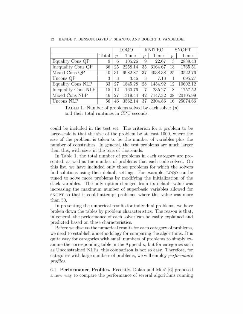
Equality Cons QP 9 6 105.26 9 22.67 3 2839.43Inequality Cons QP 36 25 2258.14 35 3164.67 13 1765.51Mixed Cons QP 40 31 9982.87 37 4038.38 25 3522.76Uncons QP 3 3 3.46 3 7.13 1 695.27Equality Cons NLP 33 27 1845.28 28 1454.92 12 10602.12Inequality Cons NLP 15 12 160.76 7 235.27 8 1757.52Mixed Cons NLP 46 27 1319.44 42 7147.32 28 20105.99Uncons NLP 56 46 3562.14 37 2304.86 16 25074.66

Table 1. Number of problems solved by each solver (p)and their total runtimes in CPU seconds.

could be included in the test set. The criterion for a problem to belarge-scale is that the size of the problem be at least 1000, where thesize of the problem is taken to be the number of variables plus thenumber of constraints. In general, the test problems are much largerthan this, with sizes in the tens of thousands.

In Table 1, the total number of problems in each category are pre-sented, as well as the number of problems that each code solved. Onthis list, we have included only those problems for which the solversfind solutions using their default settings. For example, loqo can betuned to solve more problems by modifying the initialization of theslack variables. The only option changed from its default value wasincreasing the maximum number of superbasic variables allowed forsnopt so that it could attempt problems where this value was morethan 50.

In presenting the numerical results for individual problems, we havebroken down the tables by problem characteristics. The reason is that,in general, the performance of each solver can be easily explained andpredicted based on these characteristics.

Before we discuss the numerical results for each category of problems,we need to establish a methodology for comparing the algorithms. It isquite easy for categories with small numbers of problems to simply ex-amine the corresponding table in the Appendix, but for categories suchas Unconstrained NLPs, this comparison is not so easy. Therefore, forcategories with large numbers of problems, we will employ performanceprofiles.

6.1. Performance Profiles. Recently, Dolan and More [6] proposeda new way to compare the performance of several algorithms running


on the same set of problems. Their approach is simply to computean estimate of the probability that an algorithm performs within amultiple of the runtime or iteration count (or any other metric) of thebest algorithm.

Assume that we are comparing the performance of ns solvers on np

problems. Assuming also that we are using runtime as the metric inthe profile, let

tp,s = runtime required to solve problem p by solver s.

Then, the performance ratio of solver s on problem p is defined by

ρp,s =tp,s

min{tp,s : 1 ≤ s ≤ ns}.

Here, we also assume that when a solver s cannot find a solution to aproblem p, ρp,s = ∞.

In order to evaluate the performance of the algorithm on the wholeset of problems, one can use the quantity

φs(τ) =1

np

size{p : 1 ≤ p ≤ np, ρp,s ≤ τ}.

The function φs : R → [0, 1] is called the performance profile and rep-resents the cumulative distribution function of the performance ratio.

We are now ready to examine the performance of each solver on the8 categories of problems. For each category, we will present severalmodels and discuss the performance of the solvers on each.

(1) Equality Constrained QP: It is clear from the results in Table2 that knitro outperforms loqo and snopt in this category.The difference between the two interior-point codes stems fromthe use of slack variables by loqo in the presence of equalityconstraints and free variables. These slack variables providenumerical stability for problems with ill-conditioned Hessiansby contributing to the diagonal of the KKT matrix. However,the large problems in our test suite are generally well-behaved,and, in the absence of slack variables, loqo can solve them intwo iterations by solving the exact Newton system and takinga full step in that direction. With slack variables, however,smaller steps are taken to keep them strictly positive, and loqoneeds several iterations to reach the optimal solution. knitrodoes not use slack variables in such cases and solves a smallersystem and can generally reach the optimal solution in less time.• dtoc3: This problem is an example of how slack variables

affect loqo’s performance on large-scale problems. It is a


Performance Profiles for Inequality Constrained QPs

0

0.2

0.4

0.6

0.8

1

1.2

0 5 10 15 20 25 30 35 40 45 50

tau

ph

i

LOQOKNITROSNOPT

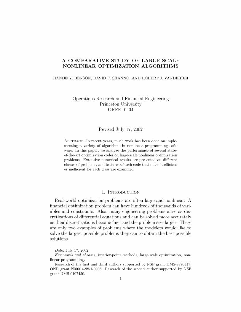
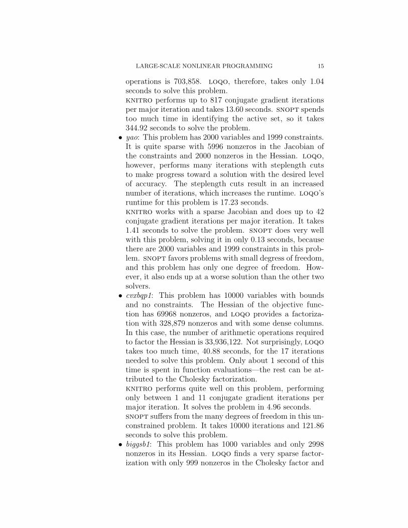
Figure 1. Performance Profiles for Inequality Con-strained QPs.

QP with 14996 variables (all of them free) and 9997 equal-ity constraints. loqo solves this problem in 10 iterationsand 23.83 seconds. When the slack variables are removedfrom the code, loqo solves this problem in 2 iterations and1.33 seconds. knitro solves this problem in 2.99 seconds,and snopt takes 597.32 seconds due to the many degreesof freedom.

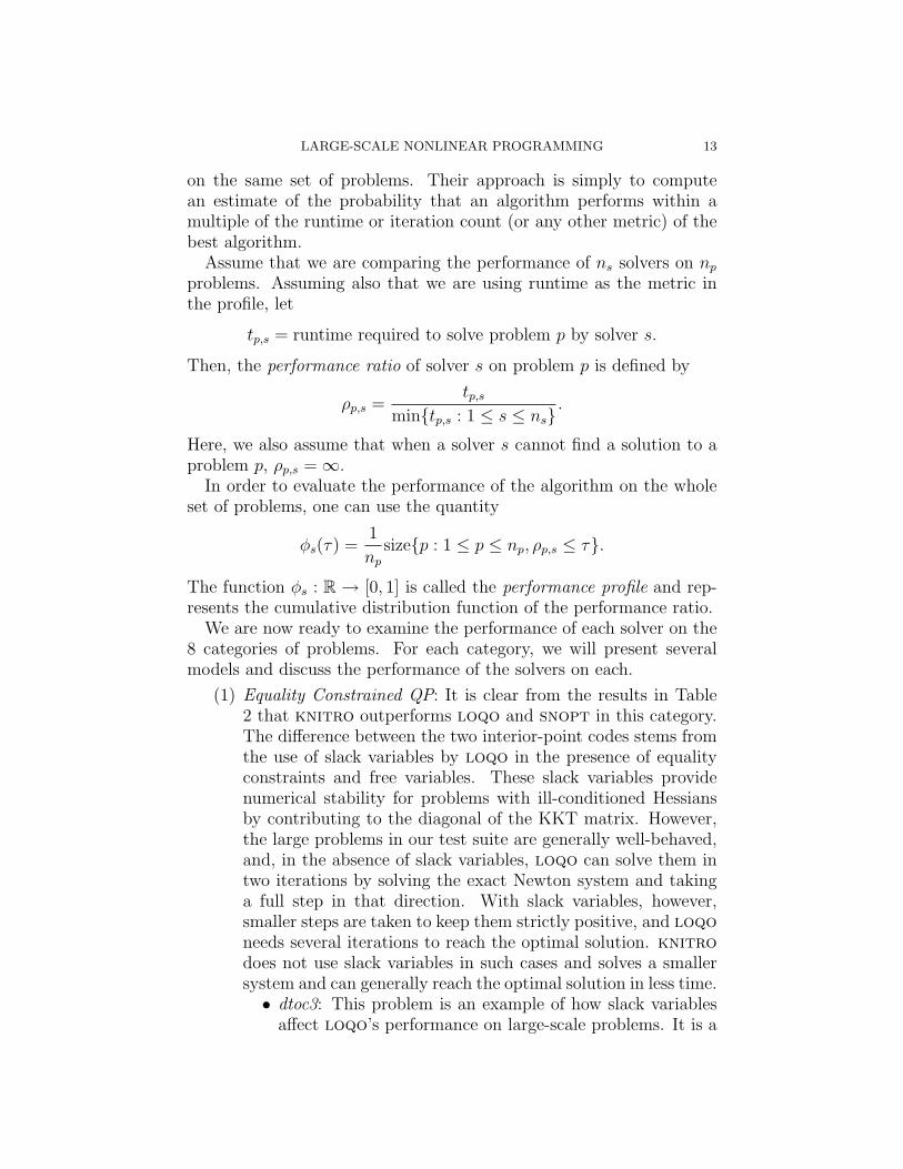
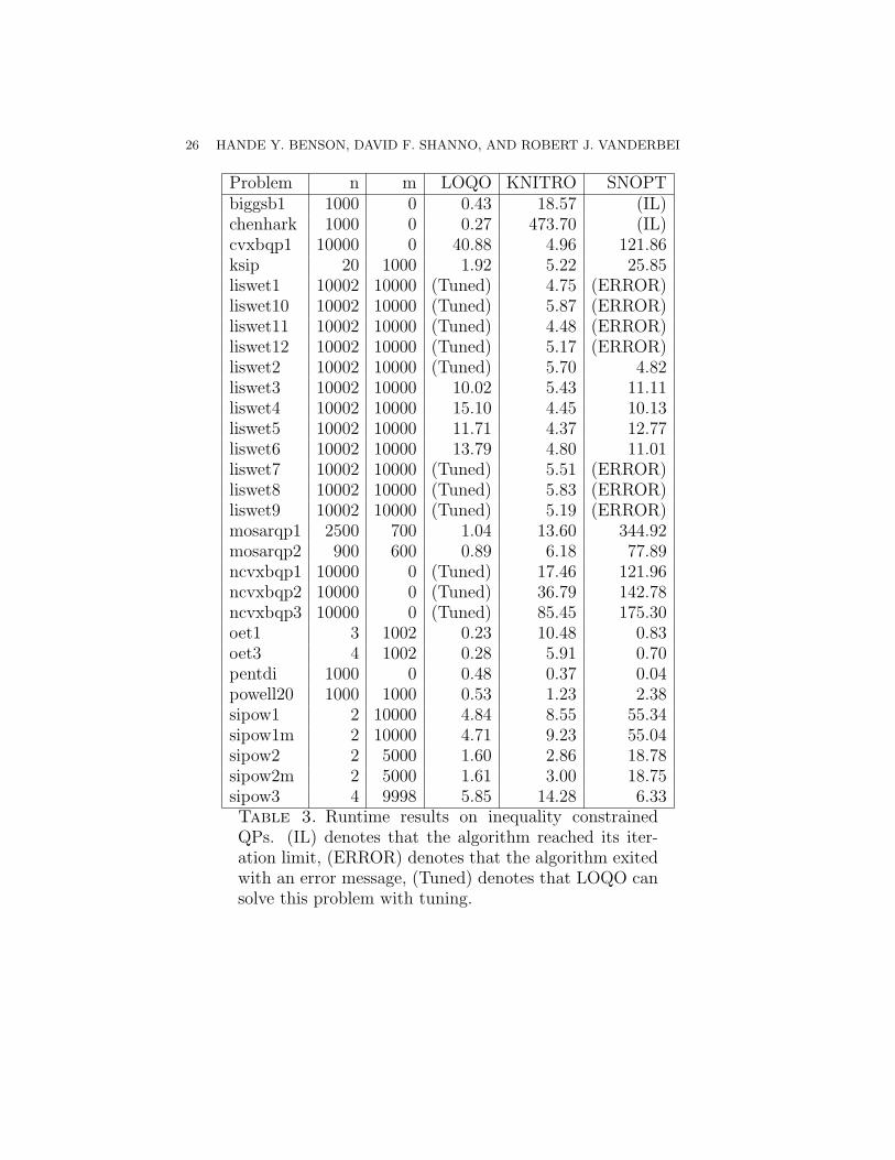
(2) Inequality Constrained QP: For these problems, loqo outper-forms knitro and snopt in most cases, but it is slow or needstuning on the liswet set. The performance profile for this cate-gory of problems is given in Figure 1.• mosarqp1: This problem has 2500 variables and 700 con-

straints. It is quite sparse, with 3422 nonzeros in the Jaco-bian of the constraints and 2590 nonzeros in the Hessian.Moreover, the Cholesky factor of the reduced KKT matrixhas 22509 nonzeros that are well-distributed throughoutthe matrix, so the estimate for the number of arithmetic


operations is 703,858. loqo, therefore, takes only 1.04seconds to solve this problem.knitro performs up to 817 conjugate gradient iterationsper major iteration and takes 13.60 seconds. snopt spendstoo much time in identifying the active set, so it takes344.92 seconds to solve the problem.

• yao: This problem has 2000 variables and 1999 constraints.It is quite sparse with 5996 nonzeros in the Jacobian ofthe constraints and 2000 nonzeros in the Hessian. loqo,however, performs many iterations with steplength cutsto make progress toward a solution with the desired levelof accuracy. The steplength cuts result in an increasednumber of iterations, which increases the runtime. loqo’sruntime for this problem is 17.23 seconds.knitro works with a sparse Jacobian and does up to 42conjugate gradient iterations per major iteration. It takes1.41 seconds to solve the problem. snopt does very wellwith this problem, solving it in only 0.13 seconds, becausethere are 2000 variables and 1999 constraints in this prob-lem. snopt favors problems with small degress of freedom,and this problem has only one degree of freedom. How-ever, it also ends up at a worse solution than the other twosolvers.

• cvxbqp1: This problem has 10000 variables with boundsand no constraints. The Hessian of the objective func-tion has 69968 nonzeros, and loqo provides a factoriza-tion with 328,879 nonzeros and with some dense columns.In this case, the number of arithmetic operations requiredto factor the Hessian is 33,936,122. Not surprisingly, loqotakes too much time, 40.88 seconds, for the 17 iterationsneeded to solve this problem. Only about 1 second of thistime is spent in function evaluations—the rest can be at-tributed to the Cholesky factorization.knitro performs quite well on this problem, performingonly between 1 and 11 conjugate gradient iterations permajor iteration. It solves the problem in 4.96 seconds.snopt suffers from the many degrees of freedom in this un-constrained problem. It takes 10000 iterations and 121.86seconds to solve this problem.

• biggsb1: This problem has 1000 variables and only 2998nonzeros in its Hessian. loqo finds a very sparse factor-ization with only 999 nonzeros in the Cholesky factor and


Performance Profiles for QPs with both Equality and Inequality Constraints

0

0.2

0.4

0.6

0.8

1

1.2

0 5 10 15 20 25 30 35 40 45 50

tau

ph

i

LOQO

KNITRO

SNOPT

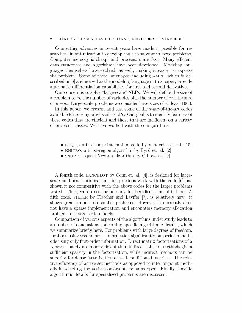
Figure 2. Performance Profiles for QPs with bothEquality and Inequality Constraints.

hence solves this problem in 0.43 seconds. knitro, on theother hand, performs up to 1469 conjugate gradient itera-tions per major iteration and takes 18.57 seconds. snoptstops when it reaches its iteration limit.

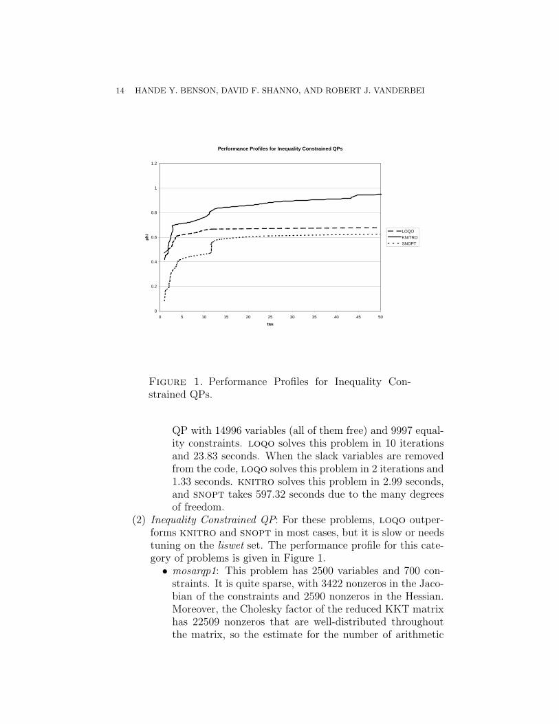
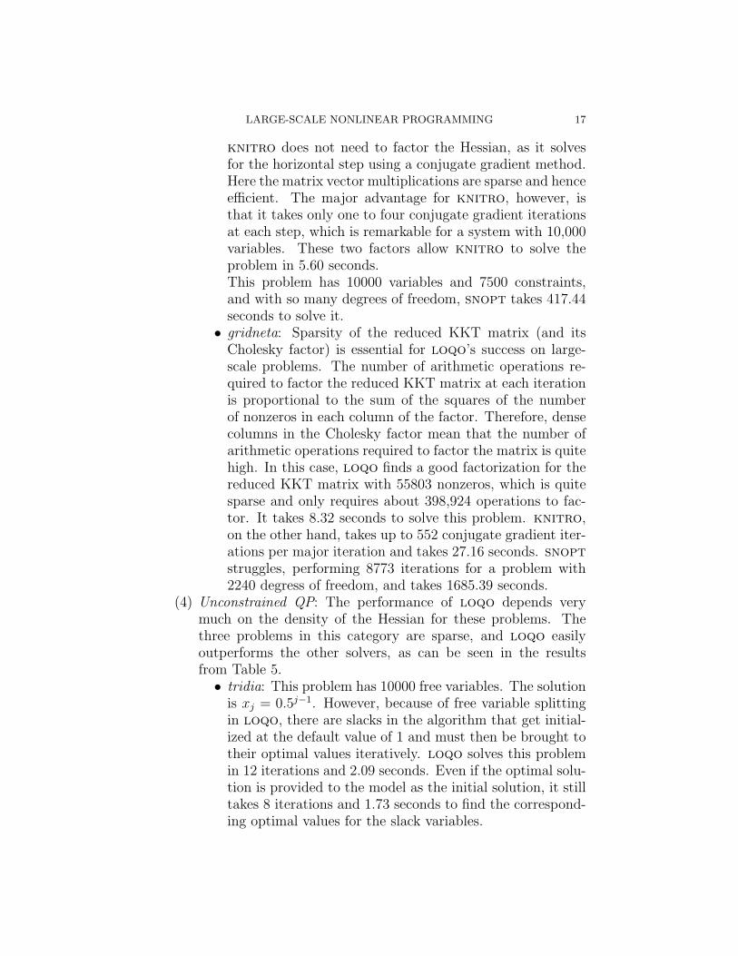
(3) QPs with both Equality and Inequality Constraints: There areseveral large sets of problems in this category, and the resultsof the comparison are mixed as can be seen in the performanceprofile in Figure 2. While knitro solves more problems withthe defaults on this category than the other two solvers, loqois able to solve the whole set with proper tuning of the slackinitialization parameter.• cvxqp3: The Jacobian of the constraints, A, and the Hes-

sian of the Lagrangian, H are both quite sparse, but thereduced KKT matrix has a dense factorization. Therefore,loqo takes 6173.21 seconds to solve the problem due tothe time required for the Cholesky factorization.


knitro does not need to factor the Hessian, as it solvesfor the horizontal step using a conjugate gradient method.Here the matrix vector multiplications are sparse and henceefficient. The major advantage for knitro, however, isthat it takes only one to four conjugate gradient iterationsat each step, which is remarkable for a system with 10,000variables. These two factors allow knitro to solve theproblem in 5.60 seconds.This problem has 10000 variables and 7500 constraints,and with so many degrees of freedom, snopt takes 417.44seconds to solve it.

• gridneta: Sparsity of the reduced KKT matrix (and itsCholesky factor) is essential for loqo’s success on large-scale problems. The number of arithmetic operations re-quired to factor the reduced KKT matrix at each iterationis proportional to the sum of the squares of the numberof nonzeros in each column of the factor. Therefore, densecolumns in the Cholesky factor mean that the number ofarithmetic operations required to factor the matrix is quitehigh. In this case, loqo finds a good factorization for thereduced KKT matrix with 55803 nonzeros, which is quitesparse and only requires about 398,924 operations to fac-tor. It takes 8.32 seconds to solve this problem. knitro,on the other hand, takes up to 552 conjugate gradient iter-ations per major iteration and takes 27.16 seconds. snoptstruggles, performing 8773 iterations for a problem with2240 degress of freedom, and takes 1685.39 seconds.

(4) Unconstrained QP: The performance of loqo depends verymuch on the density of the Hessian for these problems. Thethree problems in this category are sparse, and loqo easilyoutperforms the other solvers, as can be seen in the resultsfrom Table 5.• tridia: This problem has 10000 free variables. The solution

is xj = 0.5j−1. However, because of free variable splittingin loqo, there are slacks in the algorithm that get initial-ized at the default value of 1 and must then be brought totheir optimal values iteratively. loqo solves this problemin 12 iterations and 2.09 seconds. Even if the optimal solu-tion is provided to the model as the initial solution, it stilltakes 8 iterations and 1.73 seconds to find the correspond-ing optimal values for the slack variables.


Performance Profiles for Equality Constrained NLPs

0

0.2

0.4

0.6

0.8

1

1.2

0 5 10 15 20 25 30 35 40 45 50

tau

ph

i

LOQO

KNITRO

SNOPT

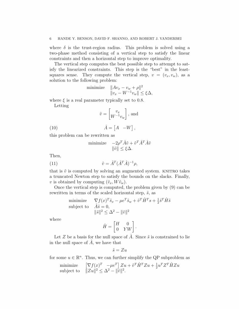
Figure 3. Performance Profiles for Equality Con-strained NLPs.

knitro solves the problem with the default initial valuein 5.72 seconds and snopt ran for several hours withoutmaking any progress, due to the many degrees of freedom.When the optimal solution is provided as the initial value,knitro exits with the error message that the step size issmaller than the machine precision, but snopt detects thatthe solution is optimal in 0 iterations and 0.40 seconds.

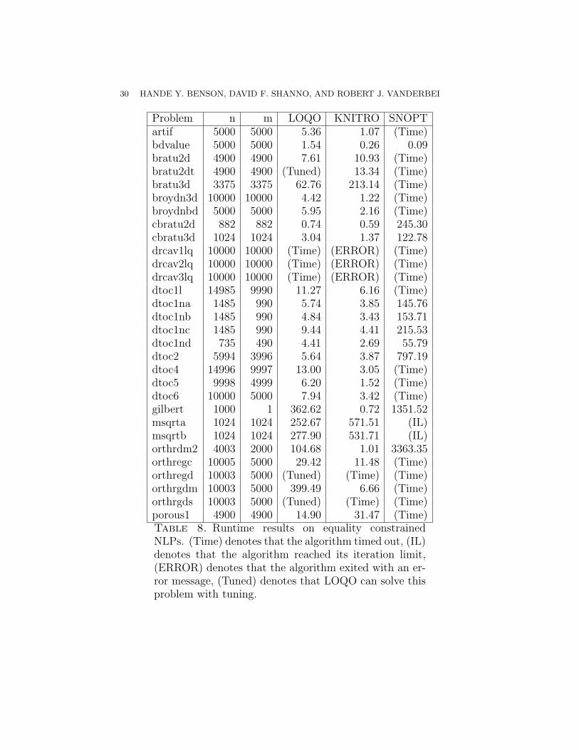
(5) Equality Constrained NLP: The performance profiles for thesolvers are given by Figure 3. knitro outperforms loqo forthis set of problems, and snopt reaches its time limit due to theeffort required by the limited-memory quasi-Newton approach.

• gilbert: This problem has one constraint that has quadraticterms for each variable. Even though the Hessian is diag-onal, the one dense row in the reduced KKT matrix fillsup the Cholesky factor when using the default settings inloqo. The resulting factor has 500500 nonzeros, and loqotakes 362.62 seconds to solve this problem. However, when


the “primal ordering” is requested, the nonzeros of the Ja-cobian cannot diffuse into the rest of the reduced KKTmatrix, so we have a problem with only 1000 nonzeros andloqo solves it in 0.73 seconds. This runtime is compara-ble to knitro’s runtime of 0.72 seconds. snopt solves thisproblem in 1351.52 seconds.

• dtoc4: This problem has an objective function with 5000terms and 4999 nonlinear equality constraints. Therefore,the evaluation times for the functions and the Hessian takeup about half of loqo’s runtime of 13.00 seconds. knitrosolves this problem in 3.05 seconds, and snopt times out.

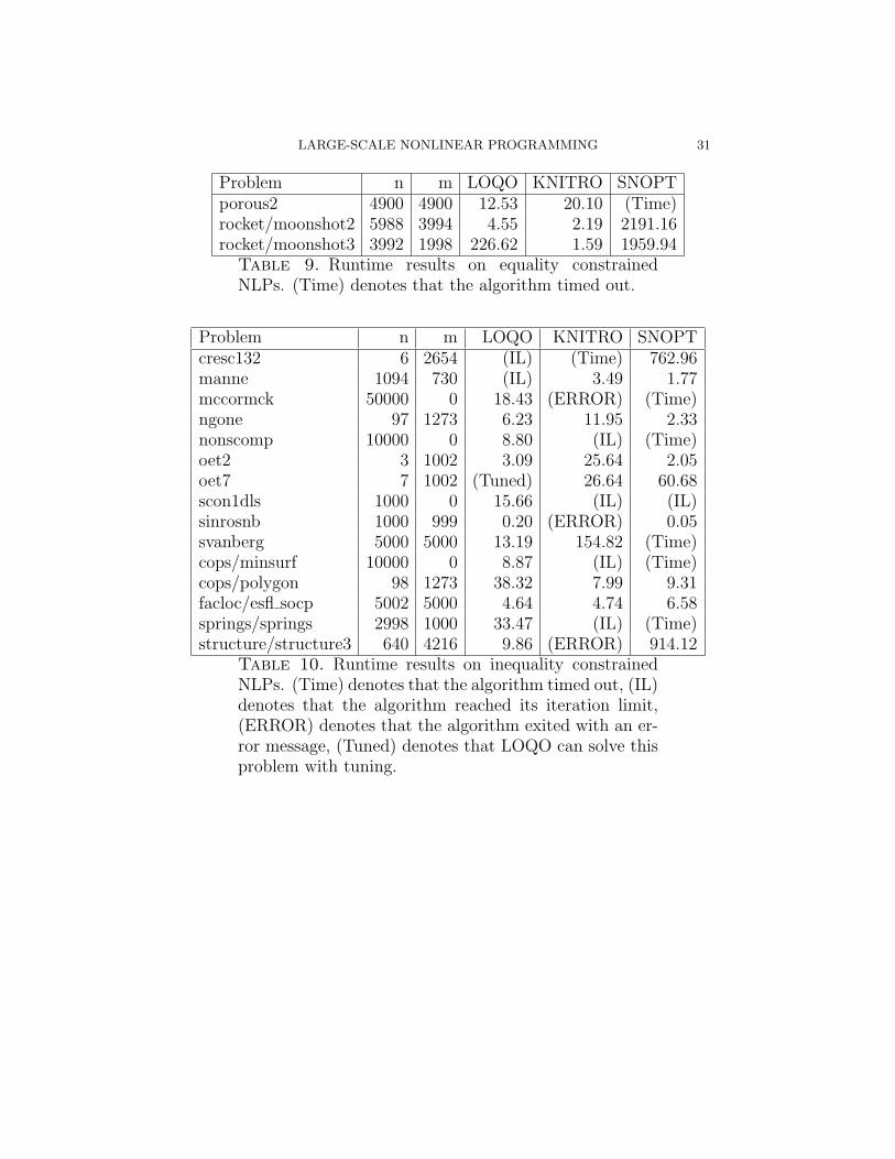
(6) Inequality Constrained NLP: As can be seen in Table 9, loqooutperforms knitro and snopt on this set of problems.• cops/polygon: loqo performs 364 iterations, most of them

with perturbations to the reduced KKT matrix and filtercuts, so it takes 38.32 seconds to solve this problem. How-ever, if a nondefault initial solution for the slack variablesis given to be 0.01, loqo then solves this problem in 37iterations and 2.72 seconds.knitro takes 7.99 seconds on this problem, and snoptsolves it in 17.34 seconds.

• svanberg: loqo solves this problem in 13.19 seconds, butknitro performs up to 1260 conjugate gradient iterationsper major iteration and takes 154.82 seconds. snopt timesout on this problem.

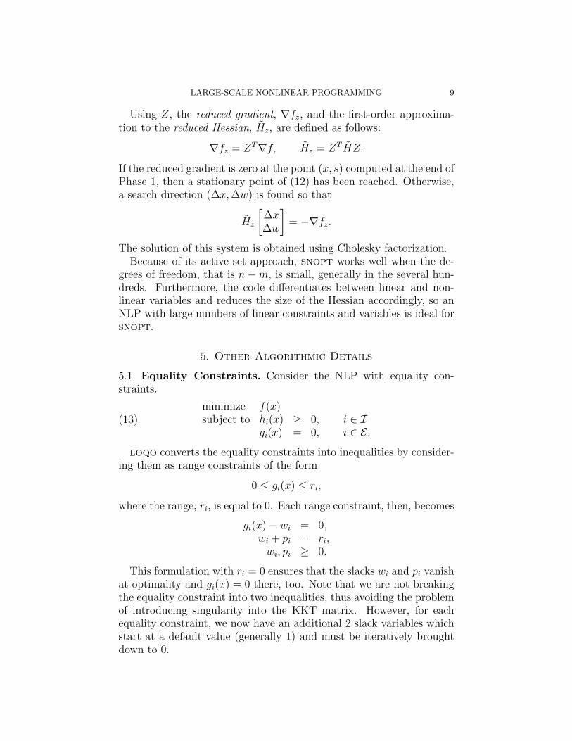
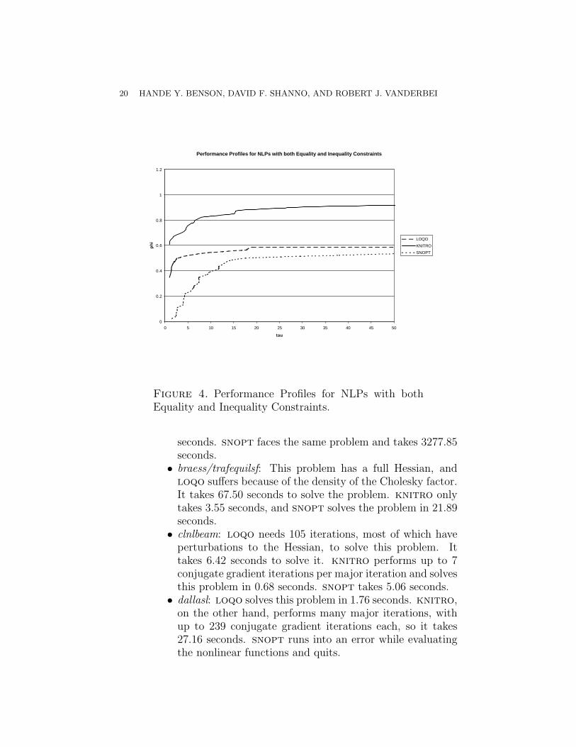
(7) NLPs with both Equality and Inequality Constraints: On thisset of problems, knitro outperforms the other solvers largelydue to the fact that it solves most of these problems on thedefaults. loqo struggles on several problem because of theinitialization of the slack variables on the equality constraints,but, given proper tuning, it solves most of these problems. Theperformance profile for this category of problems is given inFigure 4.• cops/gasoil: This problem has 20001 variables and 19998

constraints. The Jacobian of the constraints, A, is quitelarge and has 175974 nonzeros. loqo solves the problemin 186.41 seconds. However, to compute the vertical stepgiven by (11), knitro needs to first factor AT A, where A

is defined by (10). Due to the size of A and the density of

AT A, this computation requires a considerable amount oftime per iteration. knitro solves the problem in 1158.95


Performance Profiles for NLPs with both Equality and Inequality Constraints

0

0.2

0.4

0.6

0.8

1

1.2

0 5 10 15 20 25 30 35 40 45 50

tau

ph

i

LOQO

KNITRO

SNOPT

Figure 4. Performance Profiles for NLPs with bothEquality and Inequality Constraints.

seconds. snopt faces the same problem and takes 3277.85seconds.

• braess/trafequilsf: This problem has a full Hessian, andloqo suffers because of the density of the Cholesky factor.It takes 67.50 seconds to solve the problem. knitro onlytakes 3.55 seconds, and snopt solves the problem in 21.89seconds.

• clnlbeam: loqo needs 105 iterations, most of which haveperturbations to the Hessian, to solve this problem. Ittakes 6.42 seconds to solve it. knitro performs up to 7conjugate gradient iterations per major iteration and solvesthis problem in 0.68 seconds. snopt takes 5.06 seconds.

• dallasl: loqo solves this problem in 1.76 seconds. knitro,on the other hand, performs many major iterations, withup to 239 conjugate gradient iterations each, so it takes27.16 seconds. snopt runs into an error while evaluatingthe nonlinear functions and quits.


Performance Profiles for Unconstrained NLPs

0

0.2

0.4

0.6

0.8

1

1.2

0 5 10 15 20 25 30 35 40 45 50

tau

ph

i

LOQO

KNITRO

SNOPT

Figure 5. Performance Profiles for Unconstrained NLPs.

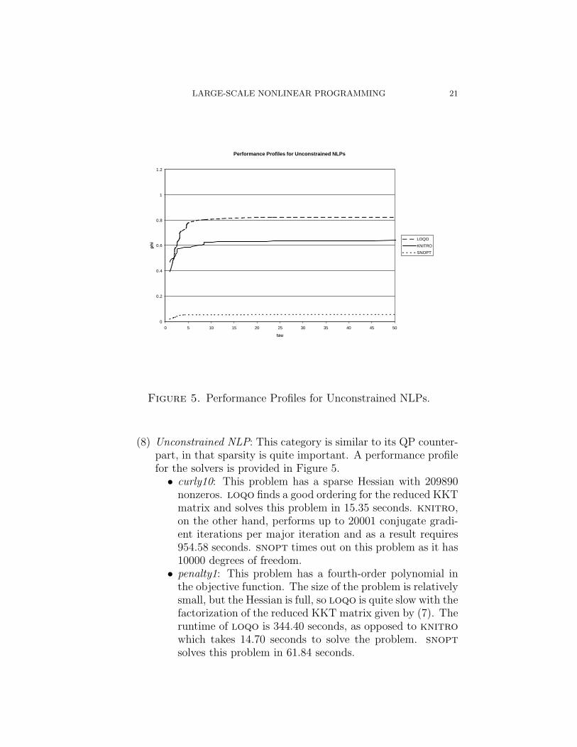
(8) Unconstrained NLP: This category is similar to its QP counter-part, in that sparsity is quite important. A performance profilefor the solvers is provided in Figure 5.• curly10: This problem has a sparse Hessian with 209890

nonzeros. loqo finds a good ordering for the reduced KKTmatrix and solves this problem in 15.35 seconds. knitro,on the other hand, performs up to 20001 conjugate gradi-ent iterations per major iteration and as a result requires954.58 seconds. snopt times out on this problem as it has10000 degrees of freedom.

• penalty1: This problem has a fourth-order polynomial inthe objective function. The size of the problem is relativelysmall, but the Hessian is full, so loqo is quite slow with thefactorization of the reduced KKT matrix given by (7). Theruntime of loqo is 344.40 seconds, as opposed to knitrowhich takes 14.70 seconds to solve the problem. snoptsolves this problem in 61.84 seconds.


7. Conclusion.

As shown in the numerical results section, each of the algorithmspresented and tested in this study has certain classes of problems onwhich they work well and others on which they perform poorly. Hereare some of the results we found after numerical testing:

• Results on sparse NLPs with sparse factorizations for the re-duced KKT matrix strongly indicate that a true Newton stepis more efficient than one employing conjugate gradients on thistype of problem.

• For dense factorizations, a conjugate gradient approach to solv-ing the Newton equations can be efficient if the matrix is suffi-ciently well-conditioned.

• For a QP with all linear equality constraints, problems shouldbe solved directly and not converted to an inequality constrainedproblem for use with an interior-point method as loqo cur-rently does. A QP with all inequality constraints, on the otherhand, is solved best using an interior-point method such asloqo. However, when the constraints are mixed (both equal-ities and inequalities), it remains to be determined whetherloqo, knitro, or an alternative approach will prove most suc-cessful in identifying the active set of the inequality constraintsand solving them most efficiently. Computational work we haveperformed for this study is inconclusive on the best way to solvethis type of problem.

• For constrained problems, loqo’s splitting of the free variableshas proved quite effective in improving the conditioning of thereduced KKT matrix [10]. For unconstrained problems, addingslacks for which initial estimates are unknown can complicatethe problem unnecessarily.

• snopt works on a reduced-space of the variables by using theconstraints, and therefore, it can efficiently solve problems withsmall degrees of freedom. Because it uses only first-order in-formation to estimate the reduced Hessian, by using a limitedmemory BFGS, the results clearly show that when the degreeof freedom is large, a quasi-Newton method is not competitivewith a Newton approach.

• For NLPs with equality constraints, the default initializationparameters for loqo often fail, as indicated by the numberof problems listed in Tables 8, 9, 11, 12 as tuned. These areproblems solved succesfully with different initial parameters.


This indicates that further research on good default setting isnecessary.

As we gain more experience in building and testing codes on a wide-variety of models, other issues might arise. So far, the results on theefficiency of state-of-the-art algorithms are quite encouraging.


References

[1] H.Y. Benson, D.F. Shanno, and R.J. Vanderbei. Interior-point methods fornonconvex nonlinear programming: Filter methods and merit functions. Tech-nical Report ORFE 00-06, Department of Operations Research and FinancialEngineering, Princeton University, 2000.

[2] R.H. Byrd, M.E. Hribar, and J. Nocedal. An interior point algorithm for largescale nonlinear programming. SIAM J. Opt., 9(4):877–900, 1999.

[3] A.R. Conn, N. Gould, and Ph.L. Toint. Constrained and unconstrained testingenvironment. http://www.dci.clrc.ac.uk/Activity.asp?CUTE.

[4] A.R. Conn, N.I.M. Gould, and Ph.L. Toint. LANCELOT: a Fortran Packagefor Large-Scale Nonlinear Optimization (Release A). Springer Verlag, Heidel-berg, New York, 1992.

[5] E. D. Dolan and J. J. More. Benchmarking optimization software with COPS.Technical Report ANL/MCS-246, Argonne National Laboratory, November2000.

[6] E. D. Dolan and J. J. More. Benchmarking optimization software with perfor-mance profiles. Math. Programming, 91:201–214, 2002.

[7] R. Fletcher and S. Leyffer. Nonlinear programming without a penalty func-tion. Technical Report NA/171, University of Dundee, Dept. of Mathematics,Dundee, Scotland, 1997.

[8] R. Fourer, D.M. Gay, and B.W. Kernighan. AMPL: A Modeling Language forMathematical Programming. Scientific Press, 1993.

[9] P.E. Gill, W. Murray, and M.A. Saunders. User’s guide for SNOPT 5.3: A For-tran package for large-scale nonlinear programming. Technical report, SystemsOptimization Laboratory, Stanford University, Stanford, CA, 1997.

[10] D.F. Shanno and R.J. Vanderbei. Interior-point methods for nonconvex non-linear programming: Orderings and higher-order methods. Math. Prog.,87(2):303–316, 2000.

[11] R.J. Vanderbei. AMPL models. http://orfe.princeton.edu/rvdb/ampl/nlmodels.[12] R.J. Vanderbei. A comparison between the minimum-local-fill and minimum-

degree algorithms. Technical report, AT&T Bell Laboratories, 1990.[13] R.J. Vanderbei. Symmetric quasi-definite matrices. SIAM Journal on Opti-

mization, 5(1):100–113, 1995.[14] R.J. Vanderbei. LOQO: An interior point code for quadratic programming.

Optimization Methods and Software, 12:451–484, 1999.[15] R.J. Vanderbei and D.F. Shanno. An interior-point algorithm for noncon-

vex nonlinear programming. Computational Optimization and Applications,13:231–252, 1999.

Hande Y. Benson, Princeton University, Princeton, NJ

David F. Shanno, Rutgers University, New Brunswick, NJ

Robert J. Vanderbei, Princeton University, Princeton, NJ


Problem n m LOQO KNITRO SNOPTaug2d 20192 9996 27.47 5.36 (Time)aug2dc 20200 9996 28.76 4.34 (Time)aug3d 3873 1000 5.54 0.78 585.03aug3dc 3873 1000 5.56 0.54 1657.08dtoc3 14996 9997 23.83 2.99 597.32gridnetb 13284 6724 14.10 4.30 (Time)hager1 10000 5000 (Tuned) 0.97 (Time)hager2 10000 5000 (Tuned) 1.54 (Time)hager3 10000 5000 (Tuned) 1.85 (Time)

Table 2. Runtime results on equality constrained QPs.(Time) denotes that the algorithm timed out, (Tuned)denotes that LOQO can solve this problem with tuning.


Problem n m LOQO KNITRO SNOPTbiggsb1 1000 0 0.43 18.57 (IL)chenhark 1000 0 0.27 473.70 (IL)cvxbqp1 10000 0 40.88 4.96 121.86ksip 20 1000 1.92 5.22 25.85liswet1 10002 10000 (Tuned) 4.75 (ERROR)liswet10 10002 10000 (Tuned) 5.87 (ERROR)liswet11 10002 10000 (Tuned) 4.48 (ERROR)liswet12 10002 10000 (Tuned) 5.17 (ERROR)liswet2 10002 10000 (Tuned) 5.70 4.82liswet3 10002 10000 10.02 5.43 11.11liswet4 10002 10000 15.10 4.45 10.13liswet5 10002 10000 11.71 4.37 12.77liswet6 10002 10000 13.79 4.80 11.01liswet7 10002 10000 (Tuned) 5.51 (ERROR)liswet8 10002 10000 (Tuned) 5.83 (ERROR)liswet9 10002 10000 (Tuned) 5.19 (ERROR)mosarqp1 2500 700 1.04 13.60 344.92mosarqp2 900 600 0.89 6.18 77.89ncvxbqp1 10000 0 (Tuned) 17.46 121.96ncvxbqp2 10000 0 (Tuned) 36.79 142.78ncvxbqp3 10000 0 (Tuned) 85.45 175.30oet1 3 1002 0.23 10.48 0.83oet3 4 1002 0.28 5.91 0.70pentdi 1000 0 0.48 0.37 0.04powell20 1000 1000 0.53 1.23 2.38sipow1 2 10000 4.84 8.55 55.34sipow1m 2 10000 4.71 9.23 55.04sipow2 2 5000 1.60 2.86 18.78sipow2m 2 5000 1.61 3.00 18.75sipow3 4 9998 5.85 14.28 6.33Table 3. Runtime results on inequality constrainedQPs. (IL) denotes that the algorithm reached its iter-ation limit, (ERROR) denotes that the algorithm exitedwith an error message, (Tuned) denotes that LOQO cansolve this problem with tuning.


Problem n m LOQO KNITRO SNOPTsipow4 4 10000 7.17 20.85 8.63tfi2 3 10000 6.62 (ERROR) 8.26yao 2000 1999 17.23 1.41 (ERROR)cops/bearing 10000 0 21.18 240.83 (Time)cops/torsion 2500 0 21.17 582.23 (Time)nnls/nnls 1200 0 2068.59 1539.96 530.03

Table 4. Runtime results on inequality constrainedQPs. (Time) denotes that the algorithm timed out, (ER-ROR) denotes that the algorithm exited with an errormessage.


Problem n m LOQO KNITRO SNOPTaug2dcqp 20200 9996 22.53 89.49 (Time)aug2dqp 20192 9996 22.99 73.71 (Time)aug3dcqp 3873 1000 2.48 22.49 869.33aug3dqp 3873 1000 2.78 20.96 196.82blockqp1 2005 1001 1.03 1.26 15.49blockqp2 2005 1001 0.72 1.77 18.18blockqp3 2005 1001 1.81 2.38 17.53blockqp4 2005 1001 1.10 1.97 18.18blockqp5 2005 1001 1.86 3.33 16.03bloweya 2002 1002 4.70 1.01 2.79bloweyb 2002 1002 8.37 1.18 1.98bloweyc 2002 1002 1.68 0.63 2.01cvxqp1 1000 500 7.03 1.73 6.03cvxqp2 10000 2500 1609.03 288.39 (Time)cvxqp3 10000 7500 6173.21 5.60 417.44gouldqp2 699 349 0.45 2.45 7.23gouldqp3 699 349 0.30 0.92 1.40gridneta 8964 6724 8.32 27.16 1685.39gridnetc 7564 3844 14.82 67.98 (Time)hager4 10000 5000 7.80 8.05 (Time)hues-mod 10000 2 41.59 (IL) (Time)huestis 10000 2 8.09 (IL) (Time)ncvxqp1 1000 500 357.97 2.17 1.63ncvxqp2 1000 500 171.22 1.82 2.60ncvxqp3 1000 500 56.48 3.09 4.96ncvxqp4 1000 250 191.04 1.61 1.48ncvxqp5 1000 250 50.23 1.70 1.63ncvxqp6 1000 250 51.29 4.08 2.75ncvxqp7 1000 750 456.35 1.81 1.98ncvxqp8 1000 750 178.97 2.91 2.21Table 5. Runtime results on QPs with both equalityand inequality constraints. (Time) denotes that the algo-rithm timed out, (IL) denotes that the algorithm reachedits iteration limit, (Tuned) denotes that LOQO can solvethis problem with tuning.


Problem n m LOQO KNITRO SNOPTncvxqp9 1000 750 104.51 2.81 4.21nnls/nnls2 1249 949 1.39 5.11 9.55reading2 15001 10000 11.26 7.69 996.02sosqp2 20000 10001 17.44 37.38 (Time)ubh1 17997 12000 27.93 3211.41 (Time)markowitz/markowitz2 1200 201 557.56 130.83 192.51stengel/ex3.3.1a 1599 1598 0.61 0.27 6.68stengel/ex3.3.1b 2399 2397 3.20 0.61 11.61stengel/ex3.3.1c 2399 2397 1.44 0.62 11.54structure/structure4 720 1537 17.86 (IL) (Time)

Table 6. Runtime results on QPs with both equalityand inequality constraints. (Time) denotes that the algo-rithm timed out, (IL) denotes that the algorithm reachedits iteration limit, (Tuned) denotes that LOQO can solvethis problem with tuning.

Problem n m LOQO KNITRO SNOPTdqdrtic 5000 0 1.18 0.39 (Time)power 1000 0 0.19 1.02 695.27tridia 10000 0 2.09 5.72 (Time)

Table 7. Runtime results on unconstrained QPs.(Time) denotes that the algorithm timed out.


Problem n m LOQO KNITRO SNOPTartif 5000 5000 5.36 1.07 (Time)bdvalue 5000 5000 1.54 0.26 0.09bratu2d 4900 4900 7.61 10.93 (Time)bratu2dt 4900 4900 (Tuned) 13.34 (Time)bratu3d 3375 3375 62.76 213.14 (Time)broydn3d 10000 10000 4.42 1.22 (Time)broydnbd 5000 5000 5.95 2.16 (Time)cbratu2d 882 882 0.74 0.59 245.30cbratu3d 1024 1024 3.04 1.37 122.78drcav1lq 10000 10000 (Time) (ERROR) (Time)drcav2lq 10000 10000 (Time) (ERROR) (Time)drcav3lq 10000 10000 (Time) (ERROR) (Time)dtoc1l 14985 9990 11.27 6.16 (Time)dtoc1na 1485 990 5.74 3.85 145.76dtoc1nb 1485 990 4.84 3.43 153.71dtoc1nc 1485 990 9.44 4.41 215.53dtoc1nd 735 490 4.41 2.69 55.79dtoc2 5994 3996 5.64 3.87 797.19dtoc4 14996 9997 13.00 3.05 (Time)dtoc5 9998 4999 6.20 1.52 (Time)dtoc6 10000 5000 7.94 3.42 (Time)gilbert 1000 1 362.62 0.72 1351.52msqrta 1024 1024 252.67 571.51 (IL)msqrtb 1024 1024 277.90 531.71 (IL)orthrdm2 4003 2000 104.68 1.01 3363.35orthregc 10005 5000 29.42 11.48 (Time)orthregd 10003 5000 (Tuned) (Time) (Time)orthrgdm 10003 5000 399.49 6.66 (Time)orthrgds 10003 5000 (Tuned) (Time) (Time)porous1 4900 4900 14.90 31.47 (Time)Table 8. Runtime results on equality constrainedNLPs. (Time) denotes that the algorithm timed out, (IL)denotes that the algorithm reached its iteration limit,(ERROR) denotes that the algorithm exited with an er-ror message, (Tuned) denotes that LOQO can solve thisproblem with tuning.


Problem n m LOQO KNITRO SNOPTporous2 4900 4900 12.53 20.10 (Time)rocket/moonshot2 5988 3994 4.55 2.19 2191.16rocket/moonshot3 3992 1998 226.62 1.59 1959.94

Table 9. Runtime results on equality constrainedNLPs. (Time) denotes that the algorithm timed out.

Problem n m LOQO KNITRO SNOPTcresc132 6 2654 (IL) (Time) 762.96manne 1094 730 (IL) 3.49 1.77mccormck 50000 0 18.43 (ERROR) (Time)ngone 97 1273 6.23 11.95 2.33nonscomp 10000 0 8.80 (IL) (Time)oet2 3 1002 3.09 25.64 2.05oet7 7 1002 (Tuned) 26.64 60.68scon1dls 1000 0 15.66 (IL) (IL)sinrosnb 1000 999 0.20 (ERROR) 0.05svanberg 5000 5000 13.19 154.82 (Time)cops/minsurf 10000 0 8.87 (IL) (Time)cops/polygon 98 1273 38.32 7.99 9.31facloc/esfl socp 5002 5000 4.64 4.74 6.58springs/springs 2998 1000 33.47 (IL) (Time)structure/structure3 640 4216 9.86 (ERROR) 914.12

Table 10. Runtime results on inequality constrainedNLPs. (Time) denotes that the algorithm timed out, (IL)denotes that the algorithm reached its iteration limit,(ERROR) denotes that the algorithm exited with an er-ror message, (Tuned) denotes that LOQO can solve thisproblem with tuning.


Problem n m LOQO KNITRO SNOPTbigbank 1773 814 1.31 64.10 (Time)brainpc0 6905 6900 (Tuned) 51.14 378.32brainpc1 6905 6900 (Tuned) 194.94 797.75brainpc2 13805 13800 (Tuned) 329.19 793.75brainpc3 6905 6900 (Tuned) 71.00 836.21brainpc4 6905 6900 (Tuned) 64.89 836.21brainpc5 6905 6900 278.39 193.01 820.16brainpc6 6905 6900 (Tuned) 199.29 795.96brainpc7 6905 6900 180.02 367.99 801.20brainpc8 6905 6900 (Tuned) 68.69 804.86brainpc9 6905 6900 (Tuned) 333.45 826.44clnlbeam 1499 1000 6.42 0.68 5.06corkscrw 8997 7000 14.22 (IL) 1611.34dallasl 837 598 1.76 27.16 (ERROR)gausselm 1495 3690 (IL) 23.18 (ERROR)gridnetd 3945 2644 7.48 10.34 48.20gridnete 7565 3844 10.30 5.77 (Time)gridnetf 7565 3844 22.72 121.22 (Time)kissing 127 903 (Tuned) 111.04 (Inf)optcdeg2 1198 799 2.01 1.41 13.89optcdeg3 1198 799 1.67 1.43 13.20reading1 10001 5000 (Tuned) 31.15 (Time)sawpath 589 782 2.82 26.30 4.35semicon1 1000 1000 (Tuned) 4.56 (IL)semicon2 1000 1000 1.94 0.68 (IL)sreadin3 10000 5000 14.55 2.70 (Time)trainf 20000 10002 59.21 891.67 (Time)trainh 20000 10002 (Tuned) 2011.92 (Time)ubh5 19997 14000 (Tuned) (IL) (Time)cops/gasoil 20001 19998 186.41 1158.95 3277.85

Table 11. Runtime results on NLPs with both equal-ity and inequality constraints. (Time) denotes that thealgorithm timed out, (Inf) denotes that the SNOPT con-cluded that the problem is infeasible, (IL) denotes thatthe algorithm reached its iteration limit, (ERROR) de-notes that the algorithm exited with an error message,(Tuned) denotes that LOQO can solve this problem withtuning.


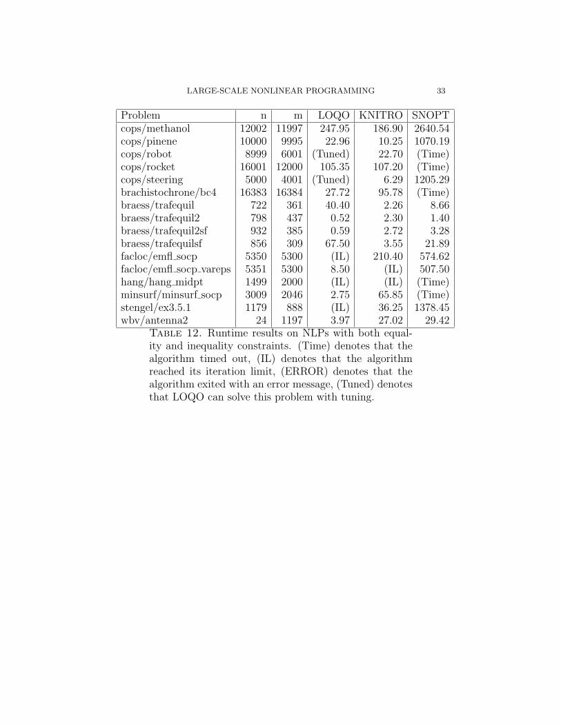
Problem n m LOQO KNITRO SNOPTcops/methanol 12002 11997 247.95 186.90 2640.54cops/pinene 10000 9995 22.96 10.25 1070.19cops/robot 8999 6001 (Tuned) 22.70 (Time)cops/rocket 16001 12000 105.35 107.20 (Time)cops/steering 5000 4001 (Tuned) 6.29 1205.29brachistochrone/bc4 16383 16384 27.72 95.78 (Time)braess/trafequil 722 361 40.40 2.26 8.66braess/trafequil2 798 437 0.52 2.30 1.40braess/trafequil2sf 932 385 0.59 2.72 3.28braess/trafequilsf 856 309 67.50 3.55 21.89facloc/emfl socp 5350 5300 (IL) 210.40 574.62facloc/emfl socp vareps 5351 5300 8.50 (IL) 507.50hang/hang midpt 1499 2000 (IL) (IL) (Time)minsurf/minsurf socp 3009 2046 2.75 65.85 (Time)stengel/ex3.5.1 1179 888 (IL) 36.25 1378.45wbv/antenna2 24 1197 3.97 27.02 29.42

Table 12. Runtime results on NLPs with both equal-ity and inequality constraints. (Time) denotes that thealgorithm timed out, (IL) denotes that the algorithmreached its iteration limit, (ERROR) denotes that thealgorithm exited with an error message, (Tuned) denotesthat LOQO can solve this problem with tuning.


Problem n m LOQO KNITRO SNOPTarwhead 5000 0 1.67 0.37 (Time)bdexp 5000 0 4.17 0.87 (Time)bdqrtic 1000 0 0.47 0.35 124.87bratu1d 1001 0 (Tuned) 1.31 (IL)broydn7d 1000 0 (IL) 2.18 1198.03brybnd 5000 0 8.44 4.14 (Time)chainwoo 1000 0 1.67 (IL) (IL)clplatea 4970 0 2.61 2.23 (Time)clplateb 4970 0 3.61 8.38 (Time)clplatec 4970 0 2.80 16.05 (Time)cosine 10000 0 3.85 (ERROR) (Time)cragglvy 5000 0 2.83 (ERROR) (Time)curly10 10000 0 15.35 954.58 (Time)curly20 10000 0 29.31 (Time) (Time)curly30 10000 0 47.16 (Time) (Time)dixmaana 3000 0 0.90 0.35 1522.23dixmaanb 3000 0 1.98 0.81 1613.16dixmaanc 3000 0 2.22 0.70 1669.69dixmaand 3000 0 2.29 0.77 1672.60dixmaane 3000 0 1.55 2.81 2667.47dixmaanf 3000 0 4.12 2.11 2656.85dixmaang 3000 0 3.51 2.08 2711.34dixmaanh 3000 0 4.13 2.13 2396.91dixmaani 3000 0 1.63 13.68 (Time)dixmaanj 3000 0 4.06 11.06 2526.37dixmaank 3000 0 4.44 11.50 (Time)dixmaanl 3000 0 4.52 9.85 3521.97dqrtic 5000 0 5.20 1.39 (Time)drcavty1 10000 0 (Time) (IL) (Time)drcavty2 10000 0 (Time) (IL) (Time)

Table 13. Runtime results on unconstrained NLPs.(Time) denotes that the algorithm timed out, (IL) de-notes that the algorithm reached its iteration limit, (ER-ROR) denotes that the algorithm exited with an errormessage, (Tuned) denotes that LOQO can solve thisproblem with tuning.


Problem n m LOQO KNITRO SNOPTdrcavty3 10000 0 (Time) (Time) (Time)edensch 2000 0 0.59 0.37 480.78engval1 5000 0 1.88 (ERROR) (Time)fletcbv3 10000 0 (ERROR) (IL) (Time)fletchbv 10000 0 (IL) (IL) (Time)fminsrf2 1024 0 (Tuned) 2.47 (Time)fminsurf 1024 0 364.16 116.48 250.41freuroth 5000 0 3.15 (ERROR) (Time)indef 1000 0 (ERROR) (IL) (Unb)liarwhd 10000 0 8.10 2.55 (Time)lminsurf 15129 0 346.25 (IL) (Time)morebv 5000 0 1.23 19.85 0.14msqrtals 1024 0 855.79 575.24 (IL)msqrtbls 1024 0 778.64 382.13 (IL)nondia 9999 0 4.63 0.82 (Time)nondquar 10000 0 6.74 57.37 (Time)penalty1 1000 0 344.40 14.70 61.84quartc 10000 0 12.47 2.69 (Time)scosine 10000 0 27.13 (IL) (Time)scurly10 10000 0 109.52 (Time) (Time)scurly20 10000 0 182.77 (Time) (Time)scurly30 10000 0 273.64 (Time) (Time)sinquad 10000 0 59.38 72.55 (Time)srosenbr 10000 0 5.01 1.91 (Time)woods 10000 0 12.17 6.03 (Time)brachistochrone/bc7 16383 0 (IL) (ERROR) (Time)

Table 14. Runtime results on unconstrained NLPs.(Time) denotes that the algorithm timed out, (IL) de-notes that the algorithm reached its iteration limit,(Unb) denotes that SNOPT reported that the problem isunbounded, (ERROR) denotes that the algorithm exitedwith an error message, (Tuned) denotes that LOQO cansolve this problem with tuning.

a comparative study of large-scale nonlinear optimization algorithms

Documents