a comparative study of covariance and precision matrix

A Comparative Study of Covariance and PrecisionMatrix Estimators for Portfolio Selection

M. Senneret1, Y. Malevergne2,3, P. Abry4, G. Perrin1, L. Jaffres1

1 Vivienne Investissement, Lyon, France2 Coactis EA 4161 – Universite de Lyon - Universite de Saint-Etienne, France

3 EMLYON Business School, France4 CNRS, ENS Lyon, France

Preliminary draft. Do not quote

Abstract

We conduct and empirical analysis of the relative performance of several estimationmethods for the covariance and the precision matrix of a large set of European stock re-turns with application to portfolio selection in the mean-variance framework. We developseveral precision matrix estimators and compare their performance to their covariance ma-trix estimators counterpart. We account for the presence of short-sale restrictions, or thelack thereof, on the optimization process and study their impact on the stability of the op-timal portfolios. We show that the best performing estimation strategy, on the basis of theex-post Sharpe ratio, does not actually depend on the fact that we choose to estimate thecovariance or the precision matrix. Nonetheless, the optimal portfolios derived from theestimated precision matrix enjoy a much lower turnover rate and concentration level evenin the absence of constraints on the investment process.

Keywords: Portfolio selection, covariance matrix, precision matrix, multivariate estima-tion, shrinkage, sparsity.

JEL Code: C13, C51, C61, G11, G15.

1 Introduction

The estimation of the covariance matrix of assets returns is an important step for a successfulimplementation of the mean-variance portfolio optimization approach (Elton and Gruber 1973,DeMiguel et al. 2009). However the estimation of large covariance matrices is a notoriouslydifficult task. Actually, if the pointwise convergence of the usual estimators is guaranteed undermild assumptions met in real-life conditions, their eigenvalues and eigenvectors often remainquite noisy, testifying of a significant loss of information during the estimation process. Be-sides, the inversion of large matrices is a tedious task, numerically unstable when the matrixis ill-conditioned as is usually the case in practice when the number of observations is (in themost favorable case) close to the number of assets under consideration. Hence matrix inversionmay contribute to add some noise during the optimization step and to make the mean-varianceapproach useless due to its tendency to maximize the effects of errors in the input assumptions(Michaud 1989). In fact, the estimation error and the numerical instability are so large thatDeMiguel et al. (2009) concluded that the naive equally-weighted investment scheme is supe-rior to the optimal asset allocation derived from the mean-variance method both in terms ofSharpe ratio and certainty equivalent. For the US stock market, based on monthly returns, theyestimated that the sample size needed for the mean-variance strategy to outperform the equally-weighted portfolio is larger than 3,000 months for a portfolio with 25 assets and 6,000 monthsfor a portfolio made of 50 assets. This should lead one to pessimistically conclude with theseauthors that “there are still many miles to go before the gains promised by optimal portfolio

choice can actually be realized out-of-sample.”

However, Ledoit and Wolf (2004b) report significantly lower ex-post variances for globalminimum-variance portfolios (GMVP) derived from shrinked sample covariance matrices com-pared with the ex-post variance of the equally-weighted portfolio or the GMVP obtained onthe basis of the raw sample covariance matrix. These findings are confirmed by Disatnik andBenninga (2007) which also suggest that the way the sample covariance matrix is shrinked isnot so important as far as the ex-post variance only is concerned. In addition to the ex-post

variance of the GMVP obtained by shrinkage methods, Jagannathan and Ma (2003) focus ontheir out-of-sample performance in terms of Sharpe ratio. Their results contrast with those ob-tained by DeMiguel et al. (2009) in so far as, in the absence of investment restrictions, theGMVP derived from the shrinkage methods exhibit ex-post Sharpe ratios larger than the one ofthe equally-weighted strategy. Hence, any hope for achievable gains from the optimal portfoliotheory is maybe not out of reach.

It is nonetheless surprising that, at the noticeable exception of the recent paper by Kourtiset al. (2012), all the efforts developed during the last decade to provide a better assessment of

1

the optimal portfolios in the mean-variance framework has been devoted to the improvement ofthe covariance matrix estimation while, in this context, the very input parameter of interest isnot the covariance matrix itself but its inverse, i.e., the so-called precision matrix. Actually, theinverse of the estimated covariance matrix is expected to provide a rather poor estimate of theprecision matrix. Not only because of the numerical instability of the inversion process, but alsobecause it is well-known that the inverse of the unbiased sample covariance matrix only pro-vides a (severely) biased estimator on the inverse covariance matrix (Muirhead 2005). Hence,for a portfolio made of 50 assets and a sample size of 100 observations, the precision matrixestimated by direct inversion of the sample covariance matrix is, on average, twice as large asthe population precision matrix. In this respect, it is important to develop reliable estimators ofthe precision matrix and to compare their accuracy, in terms of portfolio performance, with theresults obtained from the inversion of the estimated covariance matrix. It is the primary goal ofthis paper.

In addition, it seems that the introduction of restrictions on short-sales improves the per-formance of the GMVP, lowering the out-of-sample risk. It is important to understand to whatextend this result is related to the instability of the inversion of the estimated covariance matrix.Indeed, Jagannathan and Ma (2003) show that the introduction of investment restrictions actsas a shrinkage of the covariance matrix and thus leads to deal with an “effective” covariancematrix whose conditionning is better and, hence, enjoys better numerical properties and exhibitsa more suitable behavior during the optimization process. In this respect, Jagannathan and Ma(2003) suggest that the introduction of wrong constraints on the investment strategy may actu-ally help improve the portfolio performance. Pushing this argument one step further, we canwonder whether the estimation of the precision matrix still makes the addition of unnecessaryconstraints relevant or if it is enough, in and of itself, to stabilize the optimization. It is thesecondary goal of the paper.

The paper is organized as follows. In the next section, we recall the basic framework forthe mean-variance approach with and without restrictions on short-sales and we fix the mainnotations. In section 3, we present the different estimation strategies considered here. Webriefly survey relevant results for covariance matrix estimation and state new results relativeto the estimation of the precision matrix. In section 4, we report the results of our empiricalanalysis conducted on a large dataset of stocks comprised in the Euro Stoxx 600 index over thelast decade. We briefly conclude in section 5. All proofs and technical details are gathered inappendix.

2

2 Minimum variance portfolio allocation

Given a set of p risky securities, with a full-rank p×p covariance matrix of assets returns denotedby Σ, the global minimum variance portfolio without restriction on short-sales is solution to theoptimization program

w∗ = argminw w′Σw

s.t. 1′pw = 1, (1)

where 1p is the p-vector of ones and ·′ denotes the transpose operator.

The solution to the problem (1) is well-known

w∗ =Θ1p

1′pΘ1p, (2)

where Θ = Σ−1 denotes the p × p precision matrix of the assets returns. The only practicalissue we have to care about is the way to reliably estimate the weights of this portfolio. Indeedshall we prefer the estimator

w∗ =Θ1p

1′pΘ1por w∗ =

Σ−11p

1′pΣ−11p

? (3)

Intuition should suggest to prefer the first one for accuracy reasons, but common practice pro-motes the use of the second one. An obvious motivation is its ease of implementation. It istherefore important to investigate their relative properties for different estimation strategies.

Now, when short-sales are restricted, and even forbidden, the optimization program reads

w∗ = argminw w′Σw

s.t. 1′pw = 1

w ≥ 0

, (4)

where the inequality is to be taken as a generalized inequality over the nonnegative orthant.Jagannathan and Ma (2003) showed that the constraints can make the optimization problemmore robust and explain why introducing wrong constraints may help reduce the global portfoliorisk. Actually, the introduction of constraints acts as the shrinkage of the covariance matrix,which allows rationalizing the observation reported by Pantaleo et al. (2011), among others,that the choice of the covariance matrix estimator is not very important in the presence of short-sale restrictions. To understand this point, let us consider the Lagrangian of the constrainedproblem (4)

L(w, λ, ν) = w′Σw + λ(1′pw − 1

)− ν ′w, (5)

3

where λ ∈ R and ν ∈ Rp+ are the Lagrange multipliers associated to the two sets of constraints.

Writing down the Karush-Kuhn-Tucker conditions of optimality, we get

2Σw + λ · 1p − ν = 0 , (6a)

1′w − 1 = 0 , (6b)

Diag(ν)w = 0 , (6c)

w, ν ≥ 0 . (6d)

Hence equation (6a) together with equations (6b-6c) is equivalent to

2

[Σ + Diag(ν)− 1

2·(1pν

′ + ν1′p)]w + λ · 1p = 0 , (7)

so that, with a sightly different expression than the one mentioned by Jagannathan and Ma(2003), the optimal portfolio with short-sale restrictions is the same as the unconstrained opti-mal portfolio with the actual covariance matrix Σ replaced by the “effective” covariance matrixΣ + Diag(ν) − 1

2·(1pν

′ + ν1′p). This additional term leads to a decay in the effective corre-

lations between the assets. Indeed, the diagonal terms of the additional matrix are all zero, sothat the individual variances remain unchanged while the correlation between assets i and j areshifted by the amount − νi+νj

2·√

Σii·Σjj. As a consequence, the actual diversification increases and

the weights of the constrained optimal portfolio are more spread out over the different assets.

As in the absence of constraints, the solution to the constrained optimization problem in-volves the estimation of the covariance matrix or of the precision matrix. In this respect, it issensible to compare the relative performance of both approaches. The results of our empiricalstudy will be reported in section 4. Before that, let us expose the different estimation methodswe will compare.

3 Covariance and precision estimation strategies

In this section we present the main estimation approaches retained in the paper and just providea brief overview of their main properties. We refer the reader to Bai and Shi (2011) for anin-depth survey of alternative estimation strategies for the covariance matrix. We also introducenew results regarding the estimation of the precision matrix. When needed, we will refer to p asthe number of assets in the portfolio and to n as the sample size, i.e., the number of observationsfrom which the covariance/precision matrix can be estimated.

4

3.1 Direct sample estimates

The sample covariance matrix estimator is certainly the most simple estimator one can consider.However, it suffers from two main deficiencies. First of all, when the number of observationsn is less than the number of assets p, the sample covariance matrix is not full rank, hence itis not invertible. In such a case, the Moore-Penrose generalized inverse is usually retained toestimate the inverse covariance matrix. Secondly, even if the sample covariance matrix is fullrank, its inverse only provides a biased estimator of the inverse population covariance matrix.Many simple, and sometimes naive but efficient, alternatives have been proposed. Among manyothers, let us refer to the replacement of the sample covariance matrix by a scalar matrix, whichleads to the equally-weighted portfolio as the global minimum variance portfolio, or by thediagonal matrix of the sample variances or by the covariance matrix derived from a constantcorrelation model (Elton and Gruber 1973). The sample covariance matrix and its (generalized)inverse will provide the benchmark strategy for the horse race exposed in section 4.

Alternatively, in order (i) to reduce the noise in the sample covariance matrix, (ii) to geta full rank estimate of the covariance matrix even when the number of assets is larger thanthe number of observations and (iii) to get a reliable estimate of the inverse covariance ma-trix, the factor models can provide a simple approach. The simplest case is derived from theSharpe (1963) market model in which the return on the market portfolio is assumed to be thesingle relevant factor. More general models based on the Fama and French (1992) three fac-tors model or the Carhart (1997) four factors model can provide better approximations to theactual covariance matrix for stock returns. Alternatively, when the factors are unknown orunobservable, an approximate factor structure (Chamberlain and Rothschild 1983) can be re-constructed from a principal component analysis or a singular value analysis (Connor 1982, Baiand Ng 2002, Malevergne and Sornette 2004). For simplicity we will consider the single indexmarket model as representative of this second class of models:

rt = α + β · rm,t + εt, (8)

where rt denotes the p-vector of assets returns on day t ∈ {1, . . . , n}, rm,t is the return on themarket index on day t, α and β are the p-vectors of intercepts and factor loadings while εt is thep-vector of residuals with diagonal covariance matrix ∆. For simplicity, the assume the iid-nessof the observations. The covariance and precision matrices read

Σ = ∆ + σ2mββ

′ and Θ = ∆−1 − ∆−1β · β′∆−1

1σ2m

+ β′∆−1β, (9)

where σ2m = Var rm,t.

5

Based on the OLS estimate of β and the unbiased estimate of ∆, we easily get an unbiasedestimator of the covariance matrix

Σ =n− 2

n− 1· ∆ + σ2

mββ′, (10)

where σ2m is the unbiased estimate of σ2

m. We can notice that it only differs from the naiveplug-in estimator by the multiplicative factor (n− 2)/(n− 1) which becomes quickly close toone as soon as n increases. In this respect, there is no significant difference to expect betweenthis estimator and the pug-in estimator as soon as the number of observation is not ridiculouslysmall. In particular, the statistical properties of the estimator are independent from the numberof assets in portfolio.

We can also propose an alternative estimator to the plug-in estimator of the precision matrix(see Appendix B for the derivation):

Θ =n− 4

n− 2∆−1 +

(n−4n−2

)2σ2m∆−1ββ′∆−1 − 1

n−1∆−1

1 + n−4n−2

σ2mβ′∆−1β − p

n−1

. (11)

Here also, it is interesting to notice that, in the limit n goes to infinity, the estimator convergestoward the plug-in estimator but, on the contrary to the previous case, even for large n, if thenumber of assets p remains large so that p(n)/n → γ > 0, the correction in the denominatordoes not vanish and this estimator still significantly departs from the plug-in estimator.

To conclude this survey of simple estimators, let us mention the latent factors approachwhich is, to a large extend, related to the so-called random matrix theory introduced by Wigner(1953) and recently brought back to the front of the scene by Laloux et al. (1999, 2000) andtheir followers. As for the principal component analysis, the idea consists in the identificationof the eigenvalues and the eigenvectors of the covariance matrix. It is well-known that theeigenstructure of the sample covariance matrix is a highly distorted version of the populationeigenstructure unless the ratio p/n of the number of assets to the number of observations is verysmall. Indeed, the largest sample eigenvalues are larger than they should be while the smallestones are smaller. As an example, the range of the distribution of the eigenvalues of the samplecovariance matrix derived from n iid random vectors in Rp whose entries are independent stan-

dard Gaussian random variables varies between the two bounds given by(

1±√p/n)2

, in thelimit of large n and p, instead of a mass at the point 1. Hence, bias corrections are necessaryin order to squeeze the sample spectrum and make it closer to the population one. It is theseminal idea introduced by Stein (1975), Haff (1991) or more recently by El Karoui (2008). Asa consequence, we will not consider these approaches in the paper and we will just restrict to astandard PCA.

6

3.2 The shrinkage approach

The shrinkage approach is based on the minimization of a quadratic loss function. It was orig-inally introduced by Stein (1956) and provides an optimal mix between the sample estimateof the covariance/precision matrix and a target matrix. More recently, Ledoit and Wolf (2004a,2004b, 2004c) considered the shrinkage toward a scalar matrix and toward the covariance matriximplied by Sharpe’s market model while Bengtsson and Holst (2003) considered shrinking thesample covariance matrix toward the covariance matrix derived from a latent factors model es-timated by principal component analysis1. The loss function they consider is the Mean SquaredError and the optimal shrinkage parameter is such that it achieves the best trade-off between thebias and the variance of the resulting estimator. All in all, Disatnik and Benninga (2007) suggestthat the simplest approach to shrinkage provides the best results. However the recent advancesproposed by Chen et al. (2010, 2011) show that better approximations of the covariance matrixcan be obtained on the basis of improved shrinkage parameters in particular in the case wherein the input data are fat-tailed. Alternatively, non-linear shrinkage methods either based on theintroduction of an upper limit for the condition number of the estimated covariance matrix (Wonand Kim 2006, Tanaka and Nakata 2013) or on the Marcenko and Pastur (1967) equation seemto provide significant improvements (Ledoit and Peche 2011, Ledoit and Wolf 2012).

Nonetheless, we restrict our attention to the case of linear shrinkage and use the OracleApproximating Shrinkage (OAS) estimator introduced by Chen et al. (2010) for the shrinkagetoward the identity matrix since its performance is actually very close to the performance ofthe oracle shrinkage estimator, i.e., the estimator obtained when the population parameters areknown.

Lemma 1 (Chen et al. 2010, Theorem 3). Under the assumption of iid normally distributed

asset returns, given the unbiased sample covariance matrix estimator Sn, the Oracle Approxi-

mating Shrinkage estimator of the covariance matrix toward the identify matrix is

ΣOAS = ρOAS ·TrSnp· Idp + (1− ρOAS) · Sn, (12a)

ρOAS = min

(

1− 2p

)Tr (S2

n) + (TrSn)2(n− 2

p

)·[Tr (S2

n)− (TrSn)2

p

] , 1 . (12b)

The proof of this result is recalled in Appendix C as well as a generalization to the shrinkagetoward a diagonal matrix with free diagonal parameters which, to the best of our knowledge, isa new result.

1The shrinkage parameter for several classical models can be found in Schafer and Strimmer (2005).

7

The shrinkage approach can also be successfully applied to the estimation of the precisionmatrix, which may be more relevant than the application of the shrinkage to the covariancematrix itself since, as recalled in section 2, the solution to the mean-variance optimization pro-gram directly involves this former one. When the sample covariance matrix is well-conditioned,namely when the number of observations n is larger than the number of assets p, Haff (1979)provides several random shrinkage estimators that outperform the naive estimator obtained byinversion of the sample covariance matrix. The proposed strategy is, in essence, quite close tothe strategy applied by Ledoit and Wolf for the shrinkage of the covariance matrix. Now, whenthe sample covariance matrix is singular, so that the previous method does not apply, Kubokawaand Srivastava (2008) recently provides a shrinkage method to improve on the classical Moore-Penrose generalized inverse.

In the context of portfolio optimization, the shrinkage of the precision matrix has only beenrecently considered by Kourtis et al. (2012) who propose a non-parametric cross-validationmethod for the estimation of the shrinkage parameter. We depart from their approach andpropose a closed-form OAS estimator for the precision matrix when the sample covariancematrix is well-conditioned and its inverse admits a finite second order moment, i.e. n > p+ 4.

Lemma 2. Under the assumption of iid normally distributed asset returns, given the unbiased

sample precision matrix estimator Pn = n−p−2n−1

· S−1n with finite second order moment, the

Oracle Approximating Shrinkage estimator of the precision matrix toward the identify matrix is

ΘOAS = ρOAS ·TrPnp· Id + (1− ρOAS) · Pn, (13a)

ρOAS = min

n−p− 2

p(n−p−2)

n−p−1· Tr (P 2

n) +n−p−2− 2

p

n−p−1· (TrPn)2[

n−p− 2p

(n−p−2)

n−p−1+ n− p− 4

]·[Tr (P 2

n)− (TrPn)2

p

] , 1 . (13b)

We postpone the proof to Appendix C which also provides a generalization of this result tothe shrinkage toward a diagonal matrix.

The singular case is much more tedious to handle since the sample covariance matrix doesnot admit a regular inverse. The sample precision matrix is then usually estimated by help ofthe Moore-Penrose generalized inverse whose statistic follows the generalized inverse Wishartdistribution (Bodnar and Okhrin 2008). Unfortunately, to the best of our knowledge, the mo-ments of this distribution do not admit known closed-form expressions apart from the case ofcross-sectionally uncorrelated returns (Cook and Forzani 2011). Hence the derivation of theshrinkage estimator of the precision matrix in the singular case is left to future works.

8

3.3 The sparsity approach

The celebrated principle of parsimony (Occam’s razor) has also long ago been summoned forlarge covariance or precision matrices estimation (Dempster 1972, Dahl et al. 2008, Friedmanet al. 2008, Boyd et al. 2010, Cai et al. 2011, Lian 2011, e.g.). Such a calling upon parsimonyin that context may be motivated from two different origins: Either from an a priori sparsemodeling choice or from estimation issues.

Assuming a priori a sparse dependence model, i.e., the fact that, beyond the diagonal terms,only a small (compared to p(p− 1)) number of entries of covariance or precision matrices theo-retically differ from zero may first stem from some theoretical or background knowledge on thesystem governing the data at hand: Assets belonging to a given class shall be related togetherwhile assets pertaining to different classes are more likely to be independent. It then remains anopen and difficult question to decide whether such a relative independence of classes of assetsis better modeled with non diagonal zeroed entries in the covariance or in the precision matrix.When the covariance matrix is chosen sparse, its corresponding inverse, the precision matrix,is usually not sparse (and vice-versa). As a consequence, assuming that either the covarianceor the precision matrix is sparse amounts to choosing from the very beginning between twodifferent structural models. Sparse covariance is equivalent, in a Gaussian framework, to con-sider that the corresponding covariates are independent. It is likely more relevant when oneconsiders assets traded on different markets with weak cross-market correlations, thus yieldingblock-sparse covariance matrices. Conversely, sparse precision corresponds, within that sameframework, to covariates that are conditionally independent. It thus appears more naturallywhen assets returns can be assumed to be linearly related, so that given the knowledge of agiven subset, the remainders are uncorrelated. Beyond, these theoretical considerations, the nu-merical experimentations and analyses reported in Section 4 below can be read as elements ofanswers, in the context of practical portfolio allocation performance, to the challenging issue ofdeciding between a sparse a priori imposed to covariance or precision.

The second category of reasons motivating sparsity in dependence matrices stems from thewell-known screening effect that accompanies large covariance or precision matrix estimation(Hero and Rajaratnam 2011): For large matrices, estimated from short sample size, i.e., whenn & p or even when n . p, estimation performance for the non diagonal entries are suchthat it cannot be decided whether small values correspond to actual non zero correlations or toestimation fluctuations, and thus noise. Therefore, small values should be discarded and largevalues only are significantly estimated and should be further used.

In both cases – sparse modeling or estimation issues – the practical challenge is to decidehow many and which non diagonal entries should be set to zero. There have been on-going

9

efforts to address sparse matrix estimation issues, concentrating first on the precision matrix(Dempster 1972, Dahl et al. 2008, Friedman et al. 2008, Boyd et al. 2010, Cai et al. 2011, Lian2011) and more recently on the covariance matrix (Bien and Tibshirani 2011, Rothman 2012).In essence, the estimation of sparse precision matrices relies on minimizing a cost function, con-sisting of a balance between a data fidelity term associated to the precision matrix and a penaltyterm aiming at promoting sparsity. A state-of-the-art formulation of this problem is now re-ferred to as the Graphical Lasso (Friedman et al. 2008). It balances the negative log-likelihoodfunction, thus relying on the Graphical Gaussian Model framework, and hence following theoriginal formulation due to Dempster (1972), with an l1 penalization of the estimated precisionmatrix:

Θ = argminΘ

Tr(SnΘ)− log det Θ + λ · ||Θ||1, (14)

where λ denotes a penalization parameter to be selected. Indeed, l1 penalization has beenobserved to act as an efficient surrogate of l0 penalization, that explicitly counts non zero entries,yet results in a non convex optimization problem. Instead, estimating Θ from Eq. (14) thusamounts to solving a convex optimization problem, and practical solutions were described in theliterature, the two most popular relying on the so-called path-wise coordinate descent (Bien andTibshirani 2011) or Alternating Direction Method of Multipliers algorithms (Boyd et al. 2010).In the present contribution, used is made of this latter algorithm.

Sparsity can be imposed onto the covariance matrix throught the same formulation:

Σ = argminΣ

Tr(SnΣ−1) + log det Σ + λ · ||Σ||1, (15)

which however consists of a non-convex problem and is hence far more difficult to solve. It hashowever been observed that the argument in Eq. (15) can actually be split into concave and aconvex function, and that minimization can thus be performed by a majorization-minimizationalgorithm (Bien and Tibshirani 2011). The corresponding procedure has kindly been madeavailable to us by the authors of (Bien and Tibshirani 2011) and is used in Section 4.

4 Empirical results

We now turn to the implementation of the different portfolio optimization strategies on a datasetmade of the daily returns of the p = 211 stocks comprised in the Euro Stoxx 600 index be-tween December 14, 2001 and January 24, 2013. We consider both the constrained and theunconstrained optimization programs exposed in Section 2 (see Appendix D for details on theoptimization algorithms in the presence of short-sale restrictions) and different estimators of

10

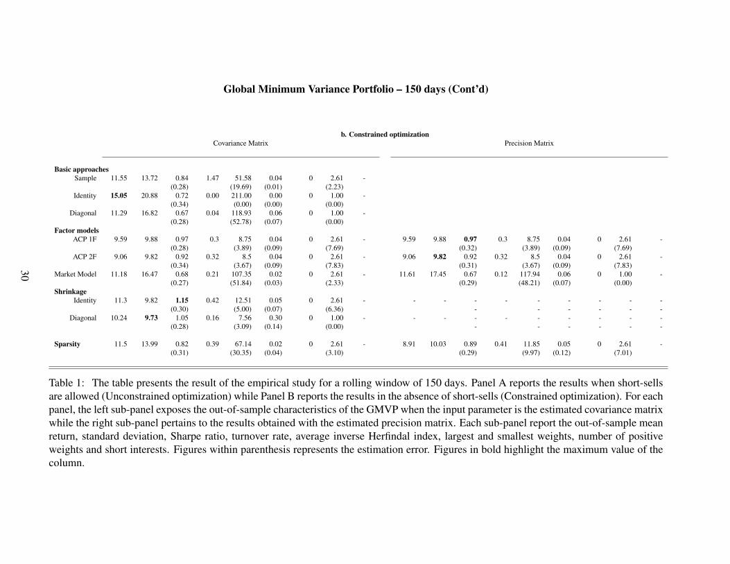
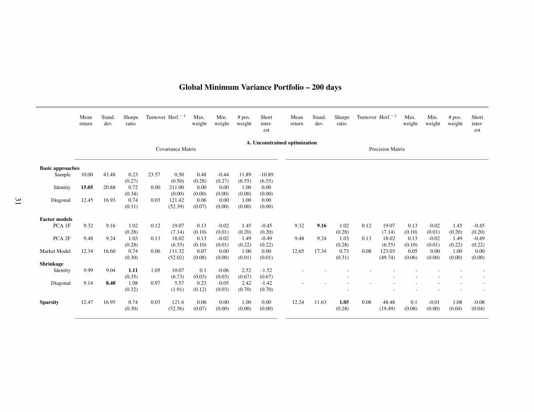
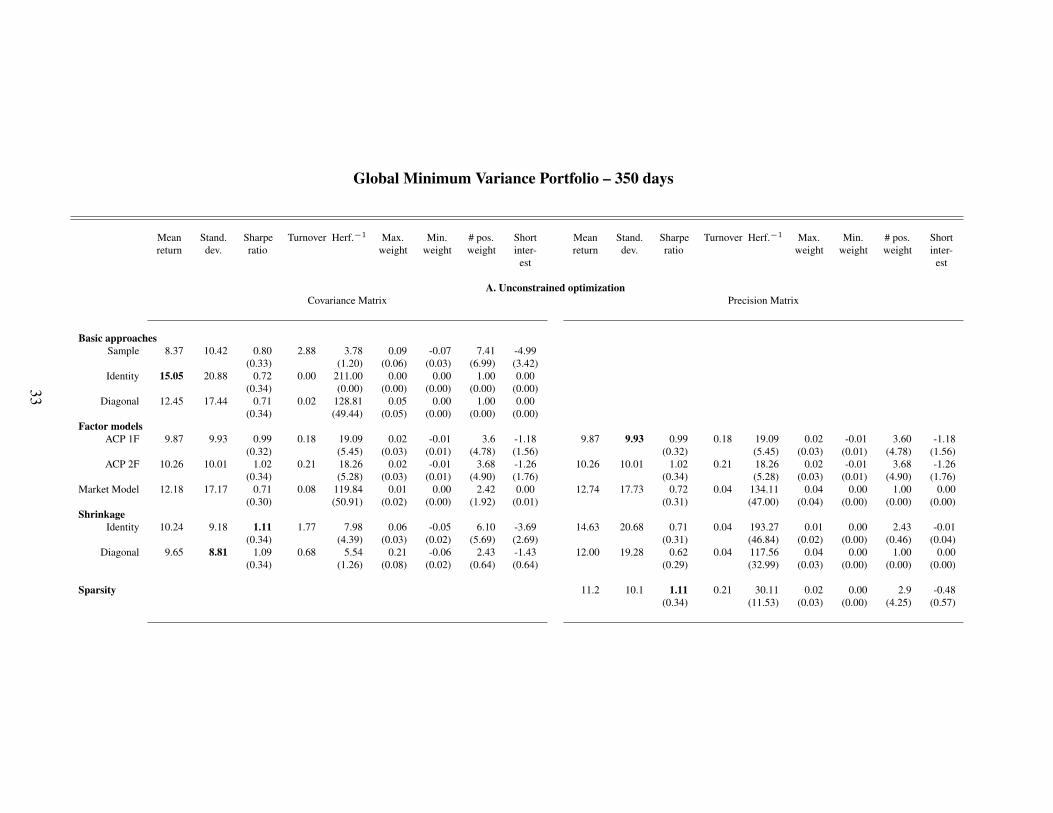
the covariance and the precision matrices. The covariance and precision matrices are estimatedover three rolling windows of size n = 150, 200 and 350 days. In the first case, the samplecovariance matrix is a highly singular matrix, in the second one a matrix near its critical pointand in the last one a full rank matrix. The portfolios, whose inception date is April 15, 2003,are rebalanced every week (five trading days). We do not account for transaction costs. Theresults are gathered in Tables 1 to 3 which report the out-of-sample performance of the optimalportfolios.

[Introduce Table 1 somewhere here]



As detailed in the previous section, we consider four classes of estimators of the covarianceand precision matrices. The first group of estimators focuses on the usual sample covarianceestimator, the identity matrix which yields the equally-weighted portfolio and the diagonal ma-trix of the sample variances. For the sample covariance matrix, the Moore-Penrose generalizedinverse is used when necessary, i.e, for rolling windows 150 and 200 days. We do not report theresults for the precision matrix since, within this group, the precision matrix estimator is (up amultiplicative factor that ensures the unbiasedness) the inverse of the corresponding covariancematrix estimator. Hence the optimization results are the same in both cases.

The second group of estimators pertains to the class of (latent) factor models. We considerthe estimators derived from a Principal Component Analysis with one and two factors, andan estimator derived from the single index market model, with the Euro Stoxx 600 index as aproxy for the market factor. In this later case, we use unrelated estimators of the covariance andthe precision matrix, i.e., the estimator of the precision matrix is not merely the inverse of thecovariance matrix estimator (see section 3.1). For the PCA-based estimators, the derivation ofspecific precision matrix estimators is left for future developments.

The third group of estimators belongs to the class of shrinkage estimators. We consider theshrinkage of the sample covariance and precision matrices toward the identity matrix (times anoverall scaling factor) and toward the diagonal matrix of the variances or precisions of eachstock. The shrinkage of the precision matrix is based on the method derived in section 3.2. Forthe time being, it requires the sample covariance matrix to be invertible. Hence, we only reportthe results obtained with a shrinked precision matrix for the rolling window of 350 days.

Finally, the fourth class of estimators is based upon the sparsity approach exposed in sec-tion 3.3 and we report both the results obtained by use of the covariance matrix and the precisionmatrix. In each case, we only report the results for the value of the penalization parameter λ

11

which leads to the smallest out-of-sample variance of the GMVP.

In terms of out-of-sample standard deviation, the shrinked covariance matrices outperformthe other covariance-based methods both with or without short-sale restrictions. Nonethelessthe superiority of the shrinkage approach diminishes with the size of the rolling window and islower in the presence of constraints. As for the precision-based approaches, both the sparsityand PCA provide the best results, depending on the length of the rolling window under con-sideration. Again, the differences between the methods tend to fade away with the length ofthe rolling window and the presence of constraints. But overall, at the noticeable exception ofthe sparse precision matrix for the rolling window of 150 days, the shrinkage of the covariancematrix alway leads to the GMVP with the lowest out-of-sample standard deviation among allthe estimation methods we have implemented in this study.

Now, regarding the performance in terms of Sharpe ratio, the shrinkage of the covariancematrix toward the identity matrix uniformly dominates of the covariance-based strategies irre-spective of the size of the rolling window and of the presence of constraints or not. We alsonotice that for the shortest rolling windows (150 and 200 days) for which for the number ofassets is larger than the sample size, the constrained optimization program leads to GMVP withhigher Sharpe ratios compared to the unconstrained case. This observation holds not only forthe best performing strategy, but for all the covariance-based strategies (at the exception of thePCA approach with two latent factors). The reverse phenomenon is observed for the longestrolling window (350 days). Hence, in line with Jagannathan and Ma (2003), we can concludethat the introduction of constraints makes the optimization process more robust when the samplecovariance matrix is ill-conditioned.

For the precision-based approaches, the sparse matrix estimation method always leads tothe highest Sharpe ratios in the absence of short-sale restrictions and still dominates in thepresence of restrictions for the longest rolling window. We do not observe that the introductionof constraints help stabilize the optimization process for small sample size. On the contrary, onaverage, the introduction of constraints spoils the performance of the GMVP. Besides when wecompare the best precision-based strategy to the best covariance-based strategy, we can onlyconclude to the lack of a significant difference. Thus, depending on the chosen approach, eitherbased on the estimation of the covariance or based on the precision matrix, the champion ofeach group is different but they lead to comparable ex-post performance.

However, if we look at the average composition of the optimal portfolios, divergences appearbetween the best performing covariance and precision-based methods. For the 150 days rollingwindow, if we compare the best performing GMVP in the absence of constraints based on bothmethods, we observe that the concentrations of the portfolios, as measured by the Herfindal

12

index (Woerheide and Persson 1993), remain close one to the other, but the turnover and theshort interest are more than three times smaller for the precision-based portfolio, which can beconsidered as a significant advantage in a practical perspective. The picture remains the samefor all rolling windows in the absence of short-sale restrictions. The composition of the bestperforming portfolio derived from the precision matrix is more stable (in terms of turnover) andexhibits lower levels of short interests. In addition, while the best performing GMVP based onthe covariance approach remains concentrated on a dozen of stocks irrespective of the size ofthe rolling window, the best performing GMVP based on the precision approach becomes lessconcentrated as the size of the rolling window increases. Of course, the introduction of short-sale restrictions naturally enforces a high-level of diversification, hence lowers the concentrationand the turnover of the portfolio, and thus rubs out the differences between the two approachesaccording to these criteria.

To sum up, our empirical results show that in terms of risk only, as measured by the out-of-sample standard deviation of the returns of the GMVP, the shrinkage of the covariance matrixdominates irrespective of the sample size and of the presence or the absence of short-sale re-strictions. Nonetheless, this lower level of out-of-sample risk does not translate into a betterout-of-sample performance, as measured by the ex-post Sharpe ratio of the GMVP. Actually,we do not observe any significant difference between the performance of the champions of thecovariance and the precision-based approaches. However, in the absence of constraints, theprecision-based approach leads to more stable GMVPs, as measured by lower concentration,lower turnover rate and lower level of short interests. Hence, as far as performance as well asrisk are concerned, the direct estimation of the precision matrix, and in particular of sparse pre-cision matrices, seems relevant for the construction of optimal portfolios from a large universeof stocks.

5 Conclusion

We have conducted an in-depth study of the relative performance of different estimation strate-gies of the GMVP based of the inversion of the estimated covariance matrix or the direct es-timation of the precision matrix. Our first contribution is the confirmation of the relevanceof the shrinkage and the positive impact of the constraints on the ex-post performance of theGMVP when focusing on the covariance-based optimization approach. However, if we confirmthe superiority of the equally-weighted portfolio in terms of raw return, it is not the case on arisk adjusted basis. More important, our analysis of the precision-based approach shows that,if the gain in terms of Sharpe ratio is not significant with respect to the standard covariance-based approach, the former leads to much more stable optimal portfolios even in the absence of

13

additional, and sometimes irrelevant, constraints.

We think that these empirical results are of interest both from an academic and a profes-sional point of view in so far as they pave the way toward the development of new estimationmethods for optimal portfolio weights in the mean-variance framework and yield new questionsregarding the informational contain of the sample covariance and precision matrices.

References

Bai, J., and S. Ng (2002) Determining the Number of Factors in Approximate Factor Models.Econometrica, 70, 191-221.

Bai, J., and S. Shi (2011) Estimating High Dimensional Covariance Matrices and its Applica-tions. Annals of Economics and Finance, 12, 199–215.

Bajeux-Besnainou, I., W. Bandara, and E. Bura (2012) A Krylov Subspace Approach to LargePortfolio Optimization. Journal of Economic Dynamics & Control 36, 1688–1699.

Bengtsson, C., and J. Holst (2003) On Portfolio Selection: Improved Covariance Matrix Esti-mation for Swedish Asset Returns. Working paper Lund University.

Bien, J., and R. J. Tibshirani (2011) Sparse Estimation of a Covariance Matrix. Biometrika 98,807–820.

Bodnar, T., and Y. Okhrin (2008) Properties of the Singular, Inverse and Generalized InversePartitioned Wishart Distributions. Journal of Multivariate Analysis 99, 2389–2405.

Boyd, S., N. Parikh, E. Chu, B. Peleato and J. Eckstein (2010) Distributed Optimization andStatistical Learning via the Alternating Direction Method of Multipliers. Foundations

and Trends in Machine Learning 3, 1-122.

Cai, T., W. Liu, and X. Luo(2011) A Constrained l1 Minimization Approach to Sparse PrecisionMatrix Estimation. Journal of the American Statistical Association 106, 594–607.

Carhart, M. M. (1997) On Persistence in Mutual Fund Performance. Journal of Finance 52,57–82.

Chamberlain, G., and M. Rothschild (1983) Arbitrage, Factor Structure and Mean-VarianceAnalysis in Large Asset Markets. Econometrica 51, 1305–1324.

Chen, Y., A. Wiesel, Y. C. Eldar and A. O. Hero (2010) Shrinkage Algorithms for MMSECovariance Estimation. IEEE Transactions on Signal Processing 58, 5016–5029.

14

Chen, Y., A. Wiesel and A. O. Hero (2011) Robust shrinkage estimation of high dimensionalcovariance matrices. IEEE Transactions on Signal Processing 59, 4097–4107.

Connor, G., (1982) Asset pricing in factor economies. Doctoral dissertation (Yale university).

Cook, R. D., and L. Forzani (2011) On the Mean and Variance of the Generalized Inverse of aSingular Wishart Matrix. Electronic Journal of Statistics 5, 146–158.

Dahl, J., L. Vandenberghe and V. Roychowdhury (2008) Covariance selection for non-chordalgraphs via chordal embedding. Optimization Methods and Software 23, 501–520.

DeMiguel, V., L. Garlappi and R. Uppal (2009) Optimal versus Naive Diversification: HowInefficient is the 1/N Portfolio Strategy? Review of Financial Studies 22, 1915–1953.

Dempster, A. P. (1972) Covariance Selection. Biometrics 28, 157–75

Desmoulins-Lebeault, F., and C. Kharoubi (2012) Non-Gaussian Diversification: When SizeMatters. Journal of Banking and Finance 36, 1987-1996.

Disatnik, D. J., and S. Benninga (2007) Shrinking the Covariance Matrix – Simpler is Better.Journal of Portfolio Management 33(4), 55–63.

El Karoui, N. (2008) Spectrum estimation for large dimensional covariance matrices using ran-dom matrix theory. Annals of Statistics, 36, 2757–2790.

Elton, E. J., and M. J. Gruber (1973) Estimating the Dependence Structure of Share Prices –Implications for Portfolio Selection, Journal of Finance 28, 1203–1232.

Evans, J., and S. Archer (1968) Diversification and the Reduction of Dispersion: An Empiricalanalysis. Journal of Finance 23, 761–767.

Fama, E. F., and K. R. French (1992) The Cross-Section of Expected Stock Returns. Journal of

Finance 47, 427–465.

Friedman, J., H. Trevor, and R. Tibshirani (2008) Sparse Inverse Covariance Estimation withthe Graphical Lasso. Biostatistics 9, 432–441.

Haff, L. R. (1979) Estimation of the Inverse Covariance Matrix: Random Mixtures of the In-verse Wishart Matrix and the Indentity. Annals of Statistics 7, 1264-1276.

Haff, L. R. (1991) The Variational Form of Certain Bayes Estimators. Annals of Statistics 19,1163–1190.

15

Hero, A. O., and B. Rajaratnam (2011) Large Scale Correlation Screening. Journal of the Amer-

ican Statistical Association 106, 1540–1552.

Jagannathan, R., and T. Ma (2003) Risk Reduction in Large Portfolios: Why Imposing theWrong Constraints Helps. Journal of Finance 58, 1651-1684.

Kourtis, A., G. Dotsis, and R. N. Markellos (2012) Parameter Uncertainty in Portfolio Selection:Shrinking the Inverse Covariance Matrix. Journal of Banking and Finance 36, 2522–2531.

Kubokawa, T. and M. S. Srivastava (2008) Estimation of the Precision Matrix of a SingularWishart Distribution and its Application in High-Dimensional Data. Journal of Multi-

variate Analysis 99, 1906–1928.

Laloux, L., P. Cizeau, J. P. Bouchaud, and M. Potters (1999). Noise Dressing of FinancialCorrelation Matrices. Physical Review Letters 83, 1467-1470.

Laloux, L., P. Cizeau, J. P. Bouchaud, and M. Potters 2000. Random Matrix Theory and Finan-cial Correlations. International Journal of Theoretical and Applied Finance 3, 391–397.

Ledoit, O. and S. Peche (2011) Eigenvectors of some large sample covariance matrix ensembles.Probability Theory and Related Fields 151, 233–264.

Ledoit, O., and M. Wolf (2004a) A Well-Conditioned Estimator for Large-Dimensional Covari-ance Matrices. Journal of Multivariate Analysis 88, 365-411.

Ledoit, O., and M. Wolf (2004b) Improved Estimation of the Covariance Matrix of Stock Re-turns With an Application to Portfolio Selection. Journal of Empirical Finance 10, 603–621.

Ledoit, O., and M. Wolf (2004c) Honey, I Shrunk the Sample Covariance Matrix. Journal of

Portfolio Management 30(4), 110–119.

Ledoit, O., and M. Wolf (2012) Nonlinear Shrinkage Estimation of Large-Dimensional Covari-ance Matrices. Annals of Statistics 40, 1024–1060.

Lian, H. (2011) Shrinkage Tuning Parameter Selection in Precision Matrices Estimation. Jour-

nal of Statistical Planning and Inference 141, 2839–2848.

Malevergne, Y., and D. Sornette (2004) Collective Origin of the Coexistence of Apparent Ran-dom Matrix Theory Noise and of Factors in Large Sample Correlation matrices. Physica

A 331, 660–668.

16

Marcenko, V. A., and Pastur, L. A. (1967). Distribution of eigenvalues for some sets of randommatrices. Sbornik: Mathematics 1, 457–483

Michaud, R. O. (1989) The Markowitz Optimization Enigma: Is ‘Optimized’ Optimal? Finan-

cial Analysts Journal 45, 31–42.

Muirhead, R. J. (2005) Aspects of Multivariate Statistical Theory (Wiley-Interscience, 2nd edi-tion)

Pantaleo, E., M. Tumminello, F. Lillo and R. N. Mantegna (2011) When do Improved Co-variance Matrix Estimators Enhance Portfolio Optimization? An Empirical ComparativeStudy of Nine Estimators. Quantitative Finance 11, 1067–1080.

Rothman, A. J. (2012) Positive definite estimators of large covariance matrices. Biometrika 99,733–740.

Schafer, J. and K. Strimmer (2005) A Shrinkage Approach to Large-Scale Covariance MatrixEstimation and Implications for Functional Genomics. Statistical Applications in Genet-

ics and Molecular Biology 4, DOI: 10.2202/1544-6115.1175.

Sharpe, W. (1963) A Simplified Model for Portfolio Analysis. Management Science 79, 277–231.

Siskind, V. (1972) Second Moments of Inverse Wishart-Matrix Elements. Biometrika 59, 690–691.

Statman, M. (1987) How Many Stocks Make a Diversified Portfolio. Journal of Financial and

Quantitative Analysis 22, 353–363.

Stein, C. (1956) Inadmissibility of the Usual Estimator for the Mean of a Multivariate NormalDistribution. Proceedings of the Third Berkeley Symposium on Mathematical Statistics

and Probability 1, 197–206.

Stein, C. (1975) Estimation of a Covariance Matrix. Rietz Lecture, 39th Annual Meeting IMS.Atlanta, Georgia.

Tanaka, M., and K. Nakata (2013) Positive definite matrix approximation with condition num-ber constraint. Optimization Letters, DOI:10.1007/s11590-013-0632-7.

Wigner, E. P. (1953) On a Class of Analytic Functions from the Quantum Theory of Collisions.Annals of Mathematics 53, 36–67.

Woerheide, W., and D. Persson (1993) An Index of Portfolio Diversification. Financial Review

Services 2, 73–85.

17

Won, J. H., and S. J. Kim (2006) Maximum likelihood covariance estimation with a conditionnumber constraint. Fortieth Asilomar Conference on Signals, Systems, and Computers,1445–1449

Yang, R. and J. 0. Berger (1994) Estimation of a Covariance Matrix Using the Reference Prior.The Annals of Statistics 22, 1195–1211.

18

A Estimation of the precision matrix in the constant correla-tion model

Under the assumption of normally distributed assets returns with values µ ∈ Rp and covariancematrix Σ, the log-likelihood of the precision matrix Θ = Σ−1 reads

log det Θ− Tr (ΘSn) , (16)

where Sn denotes the sample covariance matrix estimate from n iid random vectors of assetsreturns.

Under the constant correlation assumption, the covariance matrix reads Σ = ∆R∆ where∆ = diag(σ1, · · · , σp) and R is the correlation matrix

R = (1− ρ)Id+ ρ11t, (17)

with ρ > −1/(p− 1). By application of the Sherman-Morrison inversion formula, we get

R−1 =1

1− ρ

[Id− ρ

1 + (p− 1)ρ11t]. (18)

Thus, given that the eigenvalues of R are 1 + (p− 1)ρ and 1− ρ, with multiplicity p− 1, we get

log det Θ = log det ∆−1R−1∆−1, (19)

= 2

p∑i=1

log σ−1i − log [1 + (p− 1)ρ]− (p− 1) log(1− ρ) (20)

while

Tr (ΘSn) = Tr[∆−1R−1∆−1Sn

], (21)

= Tr[R−1∆−1Sn∆−1

], (22)

=1

1− ρTr[∆−1Sn∆−1

]− ρ

(1− ρ)[1 + (p− 1)ρ]Tr[11t∆−1Sn∆−1

], (23)

=1

1− ρTr[∆−1Sn∆−1

]− ρ

(1− ρ)[1 + (p− 1)ρ]1t∆−1Sn∆−11. (24)

19

Finally, the log likelihood reads

logL ({σi}pi=1, ρ) =

p∑i=1

log σ−1i − log [1 + (p− 1)ρ]− (p− 1) log(1− ρ)

− 1

1− ρTr[∆−1Sn∆−1

](25)

+ρ

(1− ρ)[1 + (p− 1)ρ]1t∆−1Sn∆−11.

B The one factor model

We consider the one factor model

rt = α + β · rm,t + εt, (26)

where rt denotes the p-vector of assets returns on day t ∈ {1, . . . , n}, rm,t is the return on themarket index on day t, α and β are the p-vectors of intercepts and factor loadings while εt is thep-vector of residuals with diagonal covariance matrix ∆.

The covariance and precision matrices then reads

Σ = ∆ + σ2mββ

′, (27)

The OLS estimate of the factor loading for asset i ∈ {1, . . . , p} satisfies

βi = βi +1′n (1n · r′m − rm · 1′n) εi

n · r′mrm − (1′nrm)2 , (28)

where 1n is the n-vector of ones, from which we immediately get

E[βiβj|rm

]= βiβj +

n ·∆ij

n · r′mrm − (1′nrm)2 . (29)

Hence, by the law of iterated expectations, given the unbiased estimator of σ2m

σ2m =

1

n− 1

n∑t=1

(rm,t −

1

n

n∑s=1

rm,t

)2

, (30)

=n · r′mrm − (1′nrm)2

n · (n− 1), (31)

20

we obtain, under normality,

E[σ2m · ββ′

]= E

[σ2m · E

[ββ′|rm

]]= σ2

m · ββ′ +1

n− 1∆. (32)

Thus, considering the unbiased estimator of ∆, i.e. the sum of the squared empirical residualsnormalized by (n− 2), we conclude that

Σ =n− 2

n− 1· ∆ + σ2

mββ′, (33)

is an unbiased estimator of the covariance matrix.

As for the precision matrix, which reads

Θ = ∆−1 − ∆−1β · β′∆−1

1σ2m

+ β′∆−1β, (34)

or equivalently

Θ = ∆−1 − σ2m ·∆−1β · β′∆−1

1 + σ2m · β′∆−1β

, (35)

we can improve on the basic plug-in estimator if we account for the bias of ∆−1

E[∆−1

]=n− 2

n− 4·∆−1 (36)

since each diagonal entry of ∆ follows a χ2-distribution with n− 2 degrees of freedom.

In addition, under normality, the estimators of β and ∆ are independent, hence

E

[βi · βj

∆ii ·∆jj

∣∣∣∣∣ rm]

= E[βi · βj|rm

]· E[∆−1ii |rm

]· E[∆−1jj |rm

], (37)

=

(βiβj +

n ·∆ij

n · r′mrm − (1′nrm)2

)·(n− 2

n− 4

)2

· 1

∆ii ·∆jj

, (38)

=

(n− 2

n− 4

)2

·[βi · βj

∆ii ·∆jj

+1

(n− 1) · σ2m

· ∆ij

∆ii ·∆jj

], (39)

so that, by the law of iterated expectations, we obtain

E[σ2m · ∆−1β · β′∆−1

]=

(n− 2

n− 4

)2

·[σ2m ·∆−1β · β′∆−1 +

1

(n− 1)·∆−1

](40)

21

Similarly, we can show that

E[1 + σ2

m · β′∆−1β]

= 1 +n− 2

n− 4

[σ2m · β′∆−1β +

p

n− 1

], (41)

hence an improved estimator of the precision matrix is

Θ =n− 4

n− 2∆−1 +

(n−4n−2

)2σ2m∆−1ββ′∆−1 − 1

n−1∆−1

1 + n−4n−2

σ2mβ′∆−1β − p

n−1

. (42)

C The shrinkage approach

We follow the approach of Ledoit and Wolf (2004b) and, in a first time, we apply it to the deriva-tion of the optimal shrinkage toward the identity matrix. We are thus look for the parameter ρand ν which minimizes the quadratic loss function

L(ν, ρ) = E[||ρνId+ (1− ρ)Sn − Σ||2

](43)

where ||·|| denotes the Frobenius norm while Sn denotes the unbiased sample covariance matrixestimate from n iid random vectors of Gaussian assets returns with covariance matrix Σ.

The expansion of the quadratic loss function reads

L(ν, ρ) = ρ2Tr (νId− Σ)2 + (1− ρ)2E[Tr (Sn − Σ)2] , (44)

since Sn is an unbiased estimator of Σ so that the cross-product cancels out. The differentiationwith respect to ν yields

ν =1

pTr Σ, (45)

i.e., ν is the average variance, that will be estimated as follows

ν =1

pTrSn. (46)

By substitution into the quadratic loss function we get

L(ν, ρ) = ρ2E

[Tr

(1

p(TrSn) Id− Σ

)2]

+ 2ρ(1− ρ)E

[1

pTr (Sn) · Tr (Sn − Σ)

]+ (1− ρ)2E

[Tr (Sn − Σ)2] , (47)

22

and the differentiation with respect to ρ leads, after simple algebraic manipulations, to

ρ =E [Tr (S2

n)]− Tr (Σ2)− 1pVar (TrSn)

E [Tr (S2n)]− 1

p(TrΣ)2 − 1

pVar (TrSn)

. (48)

Notice that, up to now, this derivation is totally free from the distributional properties of thesample matrix Sn apart from the absence of bias.

Let us now use the fact that the sample covariance matrix follows a Wishart distribution

(n− 1) · Sn ∼ Wp (n− 1,Σ) , (49)

so that (Muirhead 2005)

Cov(

(Sn)ij , (Sn)kl

)=

1

(n− 1)2· Cov

((n− 1) · (Sn)ij , (n− 1) · (Sn)kl

), (50)

=1

n− 1(Σik · Σjl + Σil · Σjk) . (51)

As a consequence

E[Tr(S2n

)]=

p∑i=1

E[(S2n

)ii

]=

p∑i,j=1

E[(Sn)2

ij

], (52)

=

p∑i,j=1

Var (Sn)ij︸︷︷︸Σ2ij

+ΣiiΣjj

n−1

+ E[(Sn)ij

]2

︸︷︷︸Σ2

ij

, (53)

=n

n− 1Tr(Σ2)

+1

n− 1(Tr Σ)2 , (54)

and

Var (TrSn) = Var

[p∑i=1

(Sn)ii

]=

p∑i,j=1

Cov[(Sn)ii , (Sn)jj

]︸︷︷︸

2n−1

Σ2ij

, (55)

=2

n− 1Tr(Σ2). (56)

Notice that these relations can straightforwardly be obtained by application of the Stein-Haffidentity.

23

By substitution of equations (54) and (56) in (48), we obtain

ρ =

(1− 2

p

)Tr (Σ2) + (Tr Σ)2(

n− 2p

)Tr (Σ2) +

(1− n−1

p

)(Tr Σ)2

. (57)

This expression is the same as the one given by equation (7) in Chen et al. (2010) with thereplacement n → n − 1 to account for the fact the mean value is unknown in the present case.It can be estimated by the Oracle Approximating Shrinkage (OAS) estimator

ΣOAS = ρOAS · ν · Id+ (1− ρOAS) · Sn, (58)

ρOAS = min

(

1− 2p

)Tr (S2

n) + (TrSn)2(n− 2

p

)·[Tr (S2

n)− (TrSn)2

p

] , 1 . (59)

We can notice, in passing, that there is a typo in eq. (20) of the working paper version of Chenet al. (2010); the right equation is

φ =Tr (S2

n)− (TrSn)2

p(1− 2

p

)Tr (S2

n) + (TrSn)2. (60)

As for the shrinkage estimator of the precision matrix, the quadratic loss function reads

L(ν, ρ) = E[||ρνId+ (1− ρ)Pn −Θ||2

], (61)

where Θ = Σ−1 and Pn is the unbiased sample precision matrix obtained by inversion of thesample covariance matrix Sn if n > p or is given by the Moore-Penrose generalized inverse ifn ≤ p.

The same derivations as previously yield

ν =1

pTr Θ, (62)

i.e., ν is the inverse of the harmonic mean of the individual variances, which can be estimatedby

ν =1

pTrPn. (63)

24

As a consequence,

L(ν, ρ) = ρ2E

[Tr

(1

p(TrPn) Id−Θ

)2]

+ ρ(1− ρ)E

[1

pTr (Pn) · Tr (Pn −Θ)

]+ (1− ρ)2E

[Tr (Pn −Θ)2] , (64)

and the differentiation with respect to ρ leads to

ρ =E [Tr (P 2

n)]− Tr (Θ2)− 1pVar (TrPn)

E [Tr (P 2n)]− 1

p(Tr Θ)2 − 1

pVar (TrPn)

. (65)

In the case n > p, the inverse of the sample covariance exists and the unbiased sampleestimator of the precision matrix is

Pn =n− p− 2

n− 1· S−1

n . (66)

Indeed, given1

n− p− 2· Pn = ((n− 1) · Sn)−1 ∼ W−1

p (n− 1,Θ) , (67)

whereW−1 is the inverse Wishart distribution, we immediately get

E

[1

n− p− 2· Pn

]=

1

n− p− 2·Θ, (68)

so that Pn is actually unbiasedE [Pn] = Θ. (69)

From Siskind (1972), we know that

Cov(

(Pn)ij , (Pn)kl

)= (n− p− 2)2 · Cov

(1

n− p− 2· (Pn)ij ,

1

n− p− 2· (Pn)kl

),(70)

=2 ·Θij ·Θkl + (n− p− 2) (Θik ·Θjl + Θil ·Θjk)

(n− p− 1)(n− p− 4). (71)

25

Hence

E[Tr(P 2n

)]=

p∑i=1

E[(P 2n

)ii

]=

p∑i,j=1

E[(Pn)2

ij

], (72)

=

p∑i,j=1

{Var (Pn)ij + E

[(Pn)ij

]2}, (73)

=

(n− p

(n− p− 1)(n− p− 4)+ 1

) p∑i,j=1

Θ2ij

+n− p− 2

(n− p− 1)(n− p− 4)

p∑i,j=1

Θii ·Θjj, (74)

=

(n− p

(n− p− 1)(n− p− 4)+ 1

)Tr(Θ2)

(75)

+n− p− 2

(n− p− 1)(n− p− 4)(Tr Θ)2 , (76)

(77)

and

Var (TrPn) = Var

[p∑i=1

(Pn)ii

]=

p∑i,j=1

Cov[(Pn)ii , (Pn)jj

], (78)

= 2 ·p∑

i,j=1

Θii ·Θjj + (n− p− 1) ·Θ2ij

(n− p− 1)(n− p− 4), (79)

=2 · (Tr Θ)2 + 2(n− p− 2) · Tr (Θ2)

(n− p− 1)(n− p− 4). (80)

Thus, the oracle shrinkage parameter is

ρ =

n−p− 2p

(n−p−2)

(n−p−1)(n−p−4)· Tr (Θ2) +

n−p−2− 2p

(n−p−1)(n−p−4)· (Tr Θ)2[

1 +n−p− 2

p(n−p−2)

(n−p−1)(n−p−4)

]Tr (Θ2) +

[n−p−2− 2

p

(n−p−1)(n−p−4)− 1

p

](Tr Θ)2

. (81)

In order to derive an (hopefully) efficient estimator of the oracle shrinkage parameter, we fol-low the line of Chen et al. (2010) and introduce the Oracle Approximating Shrinkage (OAS)estimator for the precision matrix:

Lemma 3 (Shrinkage toward Identity). The Oracle Approximating Shrinkage estimator of the

26

precision matrix Θ toward the identity matrix when n > p+ 2 is

ΘOAS = ρOAS ·1

pTrPn · Id+ (1− ρOAS) · Pn, (82)

ρOAS = min

n−p− 2

p(n−p−2)

n−p−1· Tr (P 2

n) +n−p−2− 2

p

n−p−1· (TrPn)2[

n−p− 2p

(n−p−2)

n−p−1+ n− p− 4

]·[Tr (P 2

n)− (TrPn)2

p

] , 1 . (83)

Proof. We follow Chen et al. (2010), and define the AOS estimator as the limit of the iterativeprocess

Θj = ρj ·1

pTrPn · Id+ (1− ρj) · Pn, (84)

and

ρj+1 =

[n−p− 2

p(n−p−2)

]Tr(ΘjPn)+

(n−p−2− 2

p

)(TrPn)2[

n−p− 2p

(n−p−2)+(n−p−1)(n−p−4)]Tr(ΘjPn)+

[n−p−2− 2

p− 1

p(n−p−1)(n−p−4)

](TrPn)2

. (85)

Thus, by substitution of (84) into (85), we get

ρj+1 =1−

[n− p− 2

p(n− p− 2)

]φ · ρj

1 + (n− p− 1)(n− p− 4)φ−[n− p− 2

p(n− p− 2)− (n− p− 1)(n− p− 4)

]φ · ρj

(86)with

φ =Tr (P 2

n)− (TrPn)2

p[n− p− 2

p(n− p− 2)

]Tr (P 2

n) +(n− p− 2− 2

p

)(TrPn)2

. (87)

Hence

limj→∞

ρj = min

1[n− p− 2

p(n− p− 2)− (n− p− 1)(n− p− 4)

]φ, 1

(88)

by the fixed-point theorem and the result follows immediately.

A similar result can be obtained for the shrinkage of the sample precision matrix toward adiagonal matrix:

Lemma 4 (Shrinkage toward diagonal). The Oracle Approximating Shrinkage estimator of the

27

precision matrix Θ toward a diagonal matrix when n > p+ 4 is

ΘOAS = ρOAS ·Diag (Pn) + (1− ρOAS) · Pn, (89)

ρOAS = min

2 · Tr(Diag (Pn)2)+ n−p

n−p−1· Tr (P 2

n) + n−p−2n−p−1

· (TrPn)2(n−pn−p−1

+ n− p− 4)·[Tr (P 2

n)− Tr(Diag (Pn)2)] , 1

. (90)

Proof. The proof follows exactly the same lines as in the case of the shrinkage toward identity.It is omitted.

D Optimization algorithm

28

Global Minimum Variance Portfolio – 150 days

Meanreturn

Stand.dev.

Sharperatio

Turnover Herf.−1 Max.weight

Min.weight

# pos.weight

Shortinter-

est

Meanreturn

Stand.dev.

Sharperatio


Min.weight

# pos.weight

Shortinter-

est

A. Unconstrained optimizationCovariance Matrix Precision Matrix

Basic approachesSample 23.29 32.44 0.72 27.69 1.62 0.47 -0.47 19.13 -16.52

(0.29) (1.65) (0.23) (0.20) (6.01) (4.15)Identity 15.05 20.88 0.72 0.00 211.00 0.00 0.00 1.00 0.00

(0.34) (0.00) (0.00) (0.00) (0.00) (0.00)Diagonal 11.29 16.79 0.67 0.04 118.38 0.06 0.00 1.00 0.00

(0.33) (52.83) (0.08) (0.00) (0.00) (0.00)Factor models

ACP 1F 8.43 9.03 0.93 0.39 19.26 0.03 -0.01 3.74 -1.14 8.43 9.03 0.93 0.39 19.26 0.03 -0.01 3.74 -1.14(0.31) (7.68) (0.05) (0.01) (5.03) (1.39) (0.26) (7.68) (0.05) (0.01) (5.03) (1.39)

ACP 2F 8.69 9.05 0.96 0.47 17.98 0.03 -0.01 3.85 -1.24 8.69 9.05 0.96 0.47 17.98 0.03 -0.01 3.85 -1.24(0.31) (7.02) (0.05) (0.01) (5.17) (1.55) (0.33) (7.02) (0.05) (0.01) (5.17) (1.55)

Market Model 11.09 16.43 0.68 0.21 106.75 0.02 0.00 2.62 -0.01 11.68 17.43 0.67 0.14 114.83 0.06 0 1.01 -0.01(0.31) (51.78) (0.03) (0.00) (2.34) (0.02) (0.30) (48.16) (0.07) (0.00) (0.03) (0.03)

ShrinkageIdentity 10.21 8.97 1.14 2.71 12.51 0.07 -0.06 6.07 -3.46 - - - - - - - - -

(0.28) (8.06) (0.02) (0.02) (4.15) (2.03) - - - - - -Diagonal 10.24 9.73 1.05 0.16 7.56 0.30 0.00 1.00 0.00 - - - - - - - - -

(0.28) (3.09) (0.14) (0.00) (0.00) (0.00) - - - - - -

Sparsity 11.3 16.81 0.67 0.09 118.54 0.01 0 2.61 0 10.37 7.81 1.33 0.76 14.94 0.03 0 3.79 -1.18(0.32) (52.99) (0.03) (0.00) (2.09) (0.00) (0.31) (5.89) (0.07) (0.00) (5.81) (1.00)

29

Global Minimum Variance Portfolio – 150 days (Cont’d)

b. Constrained optimizationCovariance Matrix Precision Matrix

Basic approachesSample 11.55 13.72 0.84 1.47 51.58 0.04 0 2.61 -

(0.28) (19.69) (0.01) (2.23)Identity 15.05 20.88 0.72 0.00 211.00 0.00 0 1.00 -

(0.34) (0.00) (0.00) (0.00)Diagonal 11.29 16.82 0.67 0.04 118.93 0.06 0 1.00 -

(0.28) (52.78) (0.07) (0.00)Factor models

ACP 1F 9.59 9.88 0.97 0.3 8.75 0.04 0 2.61 - 9.59 9.88 0.97 0.3 8.75 0.04 0 2.61 -(0.28) (3.89) (0.09) (7.69) (0.32) (3.89) (0.09) (7.69)

ACP 2F 9.06 9.82 0.92 0.32 8.5 0.04 0 2.61 - 9.06 9.82 0.92 0.32 8.5 0.04 0 2.61 -(0.34) (3.67) (0.09) (7.83) (0.31) (3.67) (0.09) (7.83)

Market Model 11.18 16.47 0.68 0.21 107.35 0.02 0 2.61 - 11.61 17.45 0.67 0.12 117.94 0.06 0 1.00 -(0.27) (51.84) (0.03) (2.33) (0.29) (48.21) (0.07) (0.00)

ShrinkageIdentity 11.3 9.82 1.15 0.42 12.51 0.05 0 2.61 - - - - - - - - - -

(0.30) (5.00) (0.07) (6.36) - - - - - -Diagonal 10.24 9.73 1.05 0.16 7.56 0.30 0 1.00 - - - - - - - - - -

(0.28) (3.09) (0.14) (0.00) - - - - - -

Sparsity 11.5 13.99 0.82 0.39 67.14 0.02 0 2.61 - 8.91 10.03 0.89 0.41 11.85 0.05 0 2.61 -(0.31) (30.35) (0.04) (3.10) (0.29) (9.97) (0.12) (7.01)

Table 1: The table presents the result of the empirical study for a rolling window of 150 days. Panel A reports the results when short-sellsare allowed (Unconstrained optimization) while Panel B reports the results in the absence of short-sells (Constrained optimization). For eachpanel, the left sub-panel exposes the out-of-sample characteristics of the GMVP when the input parameter is the estimated covariance matrixwhile the right sub-panel pertains to the results obtained with the estimated precision matrix. Each sub-panel report the out-of-sample meanreturn, standard deviation, Sharpe ratio, turnover rate, average inverse Herfindal index, largest and smallest weights, number of positiveweights and short interests. Figures within parenthesis represents the estimation error. Figures in bold highlight the maximum value of thecolumn.

30


Meanreturn

Stand.dev.

Sharperatio


Min.weight

# pos.weight

Shortinter-

est

Meanreturn

Stand.dev.

Sharperatio


Min.weight

# pos.weight

Shortinter-

est



(0.27) (0.50) (0.28) (0.27) (6.55) (6.55)Identity 15.05 20.88 0.72 0.00 211.00 0.00 0.00 1.00 0.00

(0.34) (0.00) (0.00) (0.00) (0.00) (0.00)Diagonal 12.45 16.93 0.74 0.03 121.42 0.06 0.00 1.00 0.00

(0.31) (52.39) (0.07) (0.00) (0.00) (0.00)

Factor modelsPCA 1F 9.32 9.16 1.02 0.12 19.07 0.13 -0.02 1.45 -0.45 9.32 9.16 1.02 0.12 19.07 0.13 -0.02 1.45 -0.45

(0.28) (7.14) (0.10) (0.01) (0.20) (0.20) (0.28) (7.14) (0.10) (0.01) (0.20) (0.20)PCA 2F 9.48 9.24 1.03 0.13 18.02 0.13 -0.02 1.49 -0.49 9.48 9.24 1.03 0.13 18.02 0.13 -0.02 1.49 -0.49

(0.28) (6.55) (0.10) (0.01) (0.22) (0.22) (0.28) (6.55) (0.10) (0.01) (0.22) (0.22)Market Model 12.34 16.60 0.74 0.06 111.32 0.07 0.00 1.00 0.00 12.65 17.34 0.73 0.08 123.03 0.05 0.00 1.00 0.00

(0.30) (52.02) (0.08) (0.00) (0.01) (0.01) (0.31) (49.74) (0.06) (0.00) (0.00) (0.00)Shrinkage

Identity 9.99 9.04 1.11 1.05 10.07 0.1 -0.06 2.52 -1.52 - - - - - - - - -(0.35) (6.73) (0.03) (0.03) (0.67) (0.67) - - - - - -

Diagonal 9.14 8.48 1.08 0.97 5.57 0.23 -0.05 2.42 -1.42 - - - - - - - - -(0.32) (1.91) (0.12) (0.03) (0.70) (0.70) - - - - - -

Sparsity 12.47 16.95 0.74 0.03 121.6 0.06 0.00 1.00 0.00 12.24 11.63 1.05 0.08 48.48 0.1 -0.01 1.08 -0.08(0.30) (52.56) (0.07) (0.00) (0.00) (0.00) (0.28) (19.49) (0.08) (0.00) (0.04) (0.04)

31




(0.32) (69.28) (0.05) (0.04)Identity 15.05 20.88 0.72 0.00 211.00 0.00 0 1.00 -

(0.34) (0.00) (0.00) (0.00)Diagonal 12.48 16.96 0.74 0.03 121.97 0.06 0 1 -

(0.29) (52.35) (0.07) (0.00)Factor models

PCA 1F 10.25 9.93 1.03 0.09 8.57 0.27 0 1.00 - 10.25 9.93 1.03 0.09 8.57 0.27 0 1.00 -(0.34) (3.46) (0.12) (0.00) (0.34) (3.46) (0.12) (0.00)

PCA 2F 9.84 9.89 1.00 0.09 8.38 0.27 0 1.00 - 9.84 9.89 1.00 0.09 8.38 0.27 0 1.00 -(0.33) (3.25) (0.12) (0.00) (0.33) (3.25) (0.12) (0.00)

Market Model 12.41 16.65 0.75 0.06 111.87 0.06 0 1.00 - 12.69 17.36 0.73 0.08 123.98 0.05 0 1.00 -(0.30) (52.06) (0.08) (0.00) (0.29) (49.78) (0.06) (0.00) (0.00)

ShrinkageIdentity 11.62 9.86 1.18 0.13 11.13 0.2 0 1.00 - - - - - - - - - -

(0.32) (3.60) (0.07) (0.00) (0.00) - - - - - -Diagonal 10.68 9.84 1.09 0.13 7.5 0.3 0 1.00 - - - - - - - - - -

(0.36) (2.87) (0.13) (0.00) (0.00) - - - - - -

Sparsity 12.51 14.99 0.83 0.06 93.94 0.07 0 1.00 - 12.38 12.34 1.00 0.06 48.36 0.10 0 1.00 -(0.31) (43.26) (0.07) (0.00) (0.00) (0.30) (20.31) (0.08) (0.00) (0.00)


32


Meanreturn

Stand.dev.

Sharperatio


Min.weight

# pos.weight

Shortinter-

est

Meanreturn

Stand.dev.

Sharperatio


Min.weight

# pos.weight

Shortinter-

est



(0.33) (1.20) (0.06) (0.03) (6.99) (3.42)Identity 15.05 20.88 0.72 0.00 211.00 0.00 0.00 1.00 0.00

(0.34) (0.00) (0.00) (0.00) (0.00) (0.00)Diagonal 12.45 17.44 0.71 0.02 128.81 0.05 0.00 1.00 0.00

(0.34) (49.44) (0.05) (0.00) (0.00) (0.00)Factor models

ACP 1F 9.87 9.93 0.99 0.18 19.09 0.02 -0.01 3.6 -1.18 9.87 9.93 0.99 0.18 19.09 0.02 -0.01 3.60 -1.18(0.32) (5.45) (0.03) (0.01) (4.78) (1.56) (0.32) (5.45) (0.03) (0.01) (4.78) (1.56)

ACP 2F 10.26 10.01 1.02 0.21 18.26 0.02 -0.01 3.68 -1.26 10.26 10.01 1.02 0.21 18.26 0.02 -0.01 3.68 -1.26(0.34) (5.28) (0.03) (0.01) (4.90) (1.76) (0.34) (5.28) (0.03) (0.01) (4.90) (1.76)

Market Model 12.18 17.17 0.71 0.08 119.84 0.01 0.00 2.42 0.00 12.74 17.73 0.72 0.04 134.11 0.04 0.00 1.00 0.00(0.30) (50.91) (0.02) (0.00) (1.92) (0.01) (0.31) (47.00) (0.04) (0.00) (0.00) (0.00)

ShrinkageIdentity 10.24 9.18 1.11 1.77 7.98 0.06 -0.05 6.10 -3.69 14.63 20.68 0.71 0.04 193.27 0.01 0.00 2.43 -0.01

(0.34) (4.39) (0.03) (0.02) (5.69) (2.69) (0.31) (46.84) (0.02) (0.00) (0.46) (0.04)Diagonal 9.65 8.81 1.09 0.68 5.54 0.21 -0.06 2.43 -1.43 12.00 19.28 0.62 0.04 117.56 0.04 0.00 1.00 0.00

(0.34) (1.26) (0.08) (0.02) (0.64) (0.64) (0.29) (32.99) (0.03) (0.00) (0.00) (0.00)

Sparsity 11.2 10.1 1.11 0.21 30.11 0.02 0.00 2.9 -0.48(0.34) (11.53) (0.03) (0.00) (4.25) (0.57)

33




(0.32) (2.47) (0.07) (8.11)Identity 15.05 20.88 0.72 0.00 211.00 0.00 0 1.00 -

(0.34) (0.00) (0.00) (0.00)Diagonal 12.48 17.46 0.71 0.02 129.34 0.05 0 1.00 -

(0.33) (49.34) (0.05) (0.00)Factor models

ACP 1F 8.90 10.43 0.85 0.13 8.55 0.03 0 2.42 - 8.90 10.43 0.85 0.13 8.55 0.03 0 2.42 -(0.32) (2.43) (0.06) (7.53) (0.33) (2.43) (0.06) (7.53)

ACP 2F 8.41 10.41 0.81 0.14 8.42 0.03 0 2.42 - 8.41 10.41 0.81 0.14 8.42 0.03 0 2.42 -(0.33) (2.35) (0.06) (7.62) (0.33) (2.35) (0.06) (7.62)

Market Model 12.20 17.20 0.71 0.08 120.32 0.01 0 2.42 - 12.77 17.74 0.72 0.04 134.62 0.04 0 1 -(0.30) (50.85) (0.02) (1.90) (0.29) (46.86) (0.04) (0.00)

ShrinkageIdentity 9.7 10.25 0.95 0.19 9.60 0.03 0 2.42 - 14.66 20.71 0.71 0.03 194.79 0.01 0 2.42 -

(0.31) (1.96) (0.05) (7.20) (0.33) (42.84) (0.01) (0.40)Diagonal 8.85 10.25 0.86 0.08 7.77 0.27 0 1.00 - 12.04 19.3 0.62 0.04 118.74 0.04 0 1 -

(0.34) (2.53) (0.10) (0.00) (0.34) (2.53) (0.10) (0.00)

Sparsity - 11.02 11.64 0.95 0.14 30.19 0.02 0 2.42 -(0.29) (13.20) (0.04) (4.51)


34

a comparative study of covariance and precision matrix

Documents