a comparative review of connectivity-based wireless sensor

A Comparative Review of Connectivity-Based Wireless SensorLocalization Techniques∗

Charles J. Zinsmeyer and Turgay Korkmaz†

The University of Texas at San AntonioSan Antonio, Texas, U.S.A.

{czinsmey, korkmaz}@cs.utsa.edu

Abstract

One of the key problems in Wireless Sensor Networks (WSNs) is how to identify the location ofeach node. The research community has done considerable work on this localization problem anddeveloped various techniques ranging from hardware-based ones requiring extra units (e.g., GPS,directional antennas) to software-based ones requiring only the connectivity information. In this pa-per, we present an overview of the key localization techniques and then focus on the range-free orconnectivity based approaches. After the overview, we implement and compare the performance ofconnectivity-based techniques using simulations. We show these techniques vary considerably intheir ability to localize a wireless sensor network.

Key Words: Wireless Sensor Network, Localization, Multidimensional Scaling, Force Directed,Combinatorial Delaunay Complex

1 Introduction

Intelligent wireless sensing devices are becoming ubiquitous and are being applied in many applicationsranging from environmental monitoring to animal tracking and numerous other applications. The devicesthemselves are usually small and inexpensive. They typically have limited computing resources andlimited wireless range. However, to collect and process various types of sensory data over large areas,these devices are often assembled into vast networks called Wireless Sensor Networks (WSNs), wherethe devices (nodes) communicate with a base station through other nodes.

To efficiently perform various tasks (e.g., routing, clustering, data dissemination etc.) in WSNs, thenodes and/or the base station often need to know the exact or relative locations of the other. To solvethe localization problem in WSNs, the research community has done significant amount of work undervarious assumptions [9]. Some of the early techniques that are discussed in [4] includes the followingthree techniques: (i) Triangulation, (ii) Proximity, and (iii) Scene analysis. Triangulation uses measuresbetween an unknown point and at least three known points to determine the location of the unknownpoint. Proximity attempts to measure the nearness to the known set of points. Scene analysis examines aview from a particular vantage point.

One of the key issues in all of the above techniques is how to measure the distance between thenodes. Most of the early work on localization was focused on using physical measurements such as timeof flight (TOF) or angle of arrival (AOA) to triangulate the position of a node. These techniques requireextra hardware units (e.g., GPS, directional antennas) for physical range measurement. Therefore, weclassify such techniques as hardware-based (or range-based) ones. Hardware-based approaches are notalways the best solution for locating simple and power limited wireless sensing devices. Design solutions

Journal of Internet Services and Information Security (JISIS), volume: 2, number: 1/2, pp. 59-72∗This work is supported by DoD Infrastructure Support Program for HBCU/MI, Grant: 54477-CI-ISP (UNCLASSIFIED).†Corresponding author: Dept. of Computer Science, The University of Texas at San Antonio, One UTSA Circle, San

Antonio, TX 78249, USA, Tel: +1-210-458-7346

59

A Comparative Review of Connectivity-Based Localization Techniques Zinsmeyer and Korkmaz

often try to keep node costs, size, and power consumption to a minimum. Also, the range measurementssuch as RSSI are often not accurate and are significantly affected by environmental factors. GPS isbecoming ubiquitous, but would not function for the nodes placed indoors. Clearly, there is a need fornew localization techniques that are not limited by these constraints.

In response to this, the research community has been investigating and developing new techniquesthat utilize connectivity information. We classify such techniques as connectivity-based or range-freedue to the fact that all of the work is done in software by processing the connectivity information withoutrequiring physical range measurements. These software-based techniques determine the logical positionof nodes relative to the other nodes. The calculated position resulting from these techniques is not in aphysical coordinate system such as latitude/longitude as in GPS, but a logical coordinate system perhapsan x− y coordinate system based on hop counts between nodes. The calculated logical positions willoften be a rotation, translation and/or flip from a physical position. These positions may be mapped toa physical location when anchor nodes are provided. In many cases though (e.g., routing, clustering), itmay not be necessary to determine the exact physical position of a node. In such cases, only computingrelative positions is necessary.

In this paper, we first present a review of the existing localization techniques with a special focuson software-based (connectivity-based) techniques. We then select and implement three of the proposedconnectivity-based localization techniques and compare their performances using simulations. Our maingoal here is to better understand and compare the accuracy and complexity of the proposed techniques.In general, we observed that these techniques only offer a rough localization of the nodes with positionerrors varying from 7 percent to 78 percent from the original positions. In all cases the estimated positionswere requiring at least a translation and rotation to get into a final position. To facilitate comparison, thepositions were normalized to be in the range [0, 1].

The rest of this paper is organized as follows. In Section 2, we review the localization techniques.In Section 3, we present our simulation results. In Section 4 we analyze our results and compare theconnectivity-based localization techniques. Finally, we conclude this paper and provide some directionsfor future research in Section 5.

2 WSN Localization Techniques

In essence, we divide existing localization techniques into two classes: hardware-based (range-based)ones requiring extra units (e.g., GPS, directional antennas) to measure ranges, and software-based (connectivity-based, range-free) ones processing only the connectivity information obtained from the readily availableradios without any other physical range measurement. We now review the existing techniques underthese two classes with the special emphasis on connectivity-based ones.

2.1 Hardware-based Techniques

In this subsection, we review four localization techniques utilizing various hardware units to measure therange: Time of Flight based approach, Angle Based Approach, Global Positioning System, and SignalStrength Based Approach.

2.1.1 Time of Flight Based Approach

Time of Flight (TOF) is used to measure the distance between two nodes by measuring the time it takesfor a radio or acoustical signal to move between two nodes. By measuring the time, one can computethe distances. By measuring the distance between three or more nodes and using the known position ofat least three nodes, one can use lateration to calculate the position of a fourth node in two dimensional

60


space [5]. Same ideas can be generalized to three dimensions and used for localization with the additionof another node, as described by [5].

2.1.2 Angle Based Approach

Similarly, one can use directional antennas to measure the Angle of Arrival (AOA) of a signal froma known node through angulation. Given three or more angles, the position of a fourth node can becalculated [11]. While lateration uses distance, angulation uses angle measurements.

2.1.3 Global Positioning System

The Global Positioning System or GPS is mature, relatively inexpensive and ubiquitous. It is perhapsthe most accurate mechanism for locating a device. GPS uses satellites orbiting the earth and precisemeasurement of timing signals sent from the satellites to determine position. Time of Arrival (TOA)methods require explicit synchronization within the locating system and uses a signal stamped with anabsolute time to measure the time the signal traveled from the transmitter to the receiver. Knowing thepropagation time of a signal, the distance traveled can be computed.

Time Difference of Arrival (TDOA), which is used by GPS, uses the time difference of arrival bymeasuring the time of arrival from three or more synchronized transmitters as received by a receivingstation. For GPS to function, it must have clear access to the sky to receive the GPS signals and thereforedoes not function within locations such as buildings. Like the other approaches discussed so far, GPSrequires additional hardware such as an antenna and a GPS chip. This may increase the cost, size andpower requirements of a simple wireless sensing device.

2.1.4 Signal Strength Based Approach

Received Signal Strength Indicator (RSSI) has been proposed as alternative to TOF or AOA for makingdistance measurements. The power of a signal decreases at 1/dn,n≥ 2 . Therefore, in theory, one coulduse the received signal strength to estimate the distance between nodes and use lateration to calculate theposition of the node. But, it is well known that RSSI is not an accurate indicator of distance. Environ-mental factors, such as the presences of a wall and other obstructions affect the received signal strength.Transmissions from other devices also interfere with RSSI. On the positive side, RSSI is incorporatedinto all wireless transceivers and is readily available with no additional hardware.

2.2 Software-based Techniques

In this subsection, we focus on three localization techniques utilizing connectivity information: Multidi-mensional Scaling, Force Directed, and Combinatorial Delaunay Complex. These three algorithms canbe implemented using centralized and distributed approaches.

A centralized approach involves sending connectivity information from the nodes through the net-work to a central base station where the localization algorithms are executed. If the nodes require theresulting location information, it must be forwarded back to each of the nodes in the network. Centralizedalgorithms suffer from high traffic cost and reliability (single point of failure).

In a distributed approach, each node is responsible for calculating its position within a network.Messages are often flooded throughout the underlying network so that each node can get connectivityinformation about the other nodes and calculate its own position.

In the rest of this section, we describe the centralized versions to keep the algorithmic descriptionssimple. Some work has already been done to convert them to distributed algorithms [11].

61


2.2.1 Multidimensional Scaling Algorithm

This algorithm, like others in this section, utilizes connectivity information to derive the location ofnodes in a network. Multidimensional Scaling (MDS) is a data analysis technique often used in datavisualization to uncover the similarities or dissimilarities within a data set and is taken from work done inpsychometrics and psychophysics. In our case the data set comprises the connectivity between neighborsin the network. If a measure of distance is available, then it can be incorporated as a weighting on theconnectivity.

The authors in [10] presented an algorithm called MDS-MAP which they described as a classicalmetric approach based on the work in [12]. This is the simplest case of MDS and takes a matrix contain-ing dissimilarities between pairs of items, in our case the connectivity between nodes, and computes acoordinate matrix that minimizes a loss function called strain. The result is the coordinates of the nodesin a Euclidian space. The MDS-MAP technique is summarized in the following pseudo code:

Compute MDS-MAP

Begin

Using an all pairs shortest path algorithm, estimate

the distance between each pairs of the possible nodes

producing a distance matrix

Using these distances, apply classical MDS and keep the two

largest eigenvalues and eigenvectors to build the

relative 2D map

End Compute MDS-MAP

For our work, we assumed a distance of one for a neighboring node within radio distance and did notweight the distance. Our implementation does not utilize anchor nodes. Had we utilized anchor nodes,we would have performed a third step which would use three anchor nodes to transform the relative mapinto an absolute map.

2.2.2 Force Directed Algorithm

This approach views the nodes of a network as physical elements, such as weights and springs. The nodesare modeled as forces pulling or pushing each other. The basic idea behind force directed localization isdefined as follows [1].

To embed a graph we replace the vertices by steel rings and replace each edge with a springto form a mechanical system... The vertices are placed in some initial layout and let go sothat spring forces on the rings move the system to a minimal energy state.

Force directed algorithms can be some of the most flexible algorithms for simple undirected graphs.They define a method for using an objective function for mapping each graph layout into a number thatrepresents the energy of the layout. The objective function is defined such that graph layouts in whichthe adjacent nodes are in some pre-defined distance have lower energies.

In [3] the goal of this technique was to layout an aesthetically pleasing graph. This was later inves-tigated in [2] as an approach to network localization. A total of five different force directed approacheswere investigated in [2]: Fruchterman and Reingold (FR) Kamada-Kawai, Fruchterman-Reingold RangeAlgorithm, Kamada-Kawai Range Algorithm, multi-scale Kamada-Kawai Range Algorithm, and Multi-scale Dead Reckoning.

62


In essence, the FR algorithm [3] defines two functions: an attractive force function and repulsiveforce function. The attractive force function is used for adjacent nodes and the repulsive force functionis used for non-adjacent nodes. In the algorithm, vertices in the graph are moved repeatedly until a lowenergy state is achieved. An attractive and repulsive force is computed using Equation (1).

fa(d) = d2d2/k (1)

fr(d) = −k2/d

where d is the distance between vertices and k is the empty area around a vertex. The displacement ofeach vertex is limited to maximum value with the maximum value decreasing with each iteration and ineach iteration refinement becomes finer and finer until “low energy state” of the graph is achieved. Thetechnique is summarized in the following pseudo code:

ForceDirected

Begin

While Refinement > low energy state

For each Vertex v1For each Vertex v2

if v1 and v2 are not the same vertex

d = distance between v1 and v2Compute Vertex Displacement using fr(d)

Endif

End Loop

End Loop

For each Edge Ed = edge distance

Compute Edge Displacement using fa(d)End Loop

For each Vertex vCompute New v Position Using Displacement and Refinement

End Loop

Reduce Refinement

End Loop

End ForceDirected

2.2.3 Combinatorial Delaunay Complex Algorithm

One of the problems faced by many of the algorithms is the ability to handle large networks with com-plex structures and holes. In [6] the authors proposed an approach that dealt with these problems. Theiralgorithm utilizes graph rigidity theory and higher order topological extraction to determine the positionsof the devices. The steps involved in this algorithm are:

Identify Landmarks

Begin

Compute Boundaries

Determine Medial Axis

Identify Landmarks

End Identify Landmarks

63


Compute Voronoi Diagram

Begin

Flood for Voronoi Cells

Build Voronoi Cells

Identify Voronoi Cells for Landmarks

End Compute Voronoi Diagram

Compute Delaunay Complex

Begin

Identify Witnesses

Collect Delaunay Edges

Construct Simplices

Embed landmarks

End Compute Delaunay Complex

Begin Main

Identify Landmarks

Compute Voronoi Diagram

Compute Delaunay Complex

Trilaterate Remaining Nodes

End Main

3 Results

3.1 Input Graphs

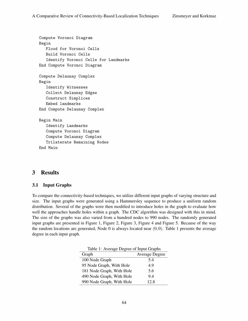
To compare the connectivity-based techniques, we utilize different input graphs of varying structure andsize. The input graphs were generated using a Hammersley sequence to produce a uniform randomdistribution. Several of the graphs were then modified to introduce holes in the graph to evaluate howwell the approaches handle holes within a graph. The CDC algorithm was designed with this in mind.The size of the graphs was also varied from a hundred nodes to 990 nodes. The randomly generatedinput graphs are presented in Figure 1, Figure 2, Figure 3, Figure 4 and Figure 5. Because of the waythe random locations are generated, Node 0 is always located near (0,0). Table 1 presents the averagedegree in each input graph.

Table 1: Average Degree of Input GraphsGraph Average Degree100 Node Graph 5.495 Node Graph, With Hole 4.9181 Node Graph, With Hole 5.6490 Node Graph, With Hole 9.4990 Node Graph, With Hole 12.8

64


Figure 1: Input Graph 1, 100 Nodes, No Hole

Figure 2: Input Graph 2, 95 nodes, 1 hole

Figure 3: Input Graph 3, 181 Nodes, 1 Hole

3.2 Output Graphs

To facilitate the comparison of the resulting localized graphs with the input graphs, the node locationswere normalized to be in the range [0 1] and the output graphs were flipped, rotated and translated so thatthe nodes roughly match the input graph. Node 0, which was located near (0,0), was used to determinethe rotation and translation offsets for the graph. So, Node 0 on the output graph was lined up with Node0 on the input graph and the resulting offset was applied to the remaining nodes.

65




3.3 Performance Metric

To measure how well a localization technique works, we compare the given node positions in the inputgraphs with the estimated node positions in the corresponding output graph, after having flipped, rotatedand/or translated the output graph. To quantify the degree of error in each output graph, we use thedistance between the original and computed position of every node, as shown in Equation (2).

Error =√

(Xoriginal−Xcomputed)2 +(Yoriginal−Ycomputed)2 (2)

We present the minimum, maximum, and average errors under each graph.

3.4 Results for Multidimensional Scaling

The output of the MDS approach was a flip and translate from the original layout. Figures 6, 7, 8, 9 and10 are the output from graph 1, graph 2, graph 3, graph 4 and graph 5, respectively. Table 2 presents theerror for each graph size. We should note that the hole present in graphs 2, 3, 4 and 5 were resolved inthe output graphs.

3.5 Results for Force Directed

The output of the force directed approach was a flip and translate from the original graph. Node 0 waslocated on the left side of the input graph and located on the right side of the output graph. Figures 11,

66


Table 2: MDS Localization ErrorGraph Average Min Max100 No Hole 0.067 0.005 0.1795, Hole 0.55 0.06 1.07200, Hole 0.72 0.06 1.07490, Hole 0.60 0.02 1.4990, Hole 0.08 0.002 0.18

Figure 6: MDS Raw Output, 100 Nodes, No Hole

Figure 7: MDS Raw Output, 95 Nodes, With Hole

12, 13, 14 and 15 are the output graphs from the force directed approach. Table 3 presents the error foreach graph size.

We note the considerable variability in the general shape of the output graphs. Input graph 3, asseen in 13, resulted in an output that resembles an hour glass and not the square layout of the originalgraph. Likewise, input graphs 4 and 5, as seen in Figures 14 and 15, resulted in outputs that visually varyconsiderably from the input graphs.

3.6 Results for Combinatorial Delaunay Complex

The output of the CDC algorithm was only a translation from the original graph. The CDC algorithmwas run on the 990 node data set only. It was noted during this work the CDC algorithm was sensitive to

67


Figure 8: MDS Raw Output, 181 Nodes, With Hole

Figure 9: MDS Raw Output 490 Nodes

Figure 10: MDS Raw Output, 990 Nodes

the initial embedding for the landmarks, including the selection of the first landmarks that are embedded.The more hops included in the initial embedding, the greater the error that was observed. This is dueto the fact that hop counts do not represent distantdistance. Figure 16 presents the output of the CDCalgorithm. Table 4 presents the error for the CDC approach.

68


Table 3: Force Directed Localization ErrorGraph Average Min Max100, No Hole 0.49 0.05 1.1995, Hole 0.06 0.004 0.16200, Hole 0.79 0.02 1.33490, Hole 0.48 0.01 1.08990, Hole 0.23 0.01 0.74

Figure 11: Force Directed Raw Output, 100 Nodes, No Hole

Figure 12: Force Directed Raw Output, 95 Nodes, No Hole

4 Analysis

All of the localization techniques focused on in this paper are based on connectivity. As such, thesetechniques do not resolve to an embedding within physical dimensions. Also, unless anchors are pro-vided, the resulted embedding may be offset by a rotation, translation or mirror from the actual layout.Nevertheless, these techniques can be useful when it is impractical to include the necessary hardwarerequired by other approaches.

We compare the average errors of the three localization techniques in Table 5. The MDS approachperformed the best for the 100 nodes no hole and 990 nodes with hole. It performed well for the 990-nodegraph, even resolving the hole as seen in Figure 10. Force directed performed better than MDS with 95nodes with a hole and slightly better than 490 nodes with a hole, though the error was significant. The

69


Figure 13: Force Directed Raw Output, 181 Nodes, Hole



CDC approach performed poorer than the MDS approach and roughly the same as the Force directed. Itdid not resolve the hole well. It should be noted that CDC works best on larger graphs [6].

These algorithms were implemented as centralized approach. So we assume that each node wouldtransmit a single packet of information containing the list of neighboring nodes back to a central com-puter that would localize the network and then transmit back the result to each node. Traffic across thenetwork would only occur when a change in the network is detected. This would work well for relativelystatic networks, but for dynamic networks, this approach would incur considerable network overhead.In such dynamic cases, the distributed approaches may work better. Some work has been done in thatdirection and we plan to evaluate their performance in our future work.

70


Table 4: CDC Localization ErrorGraph Average Min Max990, Hole 0.25 0.004 0.5

Figure 16: CDC Raw Output, 990 Nodes, Hole

5 Conclusions and Future Work

In this paper we examined localization techniques in wireless sensor networks and compared the perfor-mance of three connectivity-based algorithms: multi-dimensional scaling, force directed and combinato-rial Delaunay complex, for localizing network nodes using only connectivity information. We examinednetwork sizes up to 990 nodes with a single hole in the graph and compared the performance of thealgorithms with respect to their ability to localize the nodes. We have shown the algorithms generated anembedding that was flipped, rotated or translated relative to the input graph. We have also shown thesealgorithms vary considerably in their ability to localize a graph. Performance ranged from as good as a7 percent error to as poor as a 78 percent error.

Clearly, connectivity-based solutions are not mature enough to provide low error rate for criticalapplications. Further research is necessary to improve the performance of connectivity-based approacheswhile keeping their protocol overheads to a minimum. Specifically the graphs with holes create greatchallenges to the connectivity-based algorithms. Actually, CDC has been proposed to deal with theproblem of holes within the graph. However, it requires larger graph and its performance was not atthe desired level yet. In a follow on paper [7], the authors proposed a refinement to original work thatutilizes an incremental Delaunay refinment method which allows for a more robust algorithm that is lesssensitive to the noise results of their boundary detection. They showed the refinement performed wellwith networks of low average degree with complex shapes. Most recently the authors in [8] presented anapproach they call Approximate Convex Decomposition Localization (ACDL), which decomposes thenetwork into regularly graphs and then uses MDS approach.

Table 5: Average Localization Errors of Different TechniquesGraph Multi-Dimensional Scaling Force Directed CDC100, No Hole 0.067 0.49 —95, Hole 0.55 0.06 —200, Hole 0.72 0.79 —490, Hole 0.60 0.48 —990, Hole 0.08 0.23 0.25

71


In the future, we plan to work on new connectivity based algorithms. We also plan to expand ourstudy to the distributed version of these algorithms to determine their strengths and weakness so that en-gineers and wireless network practitioners can select the best algorithms for deployment in their systems.

References[1] P. Eades. A heuristic for graph drawing. Congressus Nutnervantiunt, 42:149–160, 1984.[2] A. Efrat, D. Forrester, A. Iyer, S. Koborouv, C. Erten, and O. Kilic. Force-directed approaches to sensor

localization. ACM Transactions on Sensor Networks, 7(3), September 2010.[3] T. M. Fruchterman and E. M. Reingold. Graph drawing by force-directed placement. Software - Practice

and Experience, 21(11):1129–1160, November 1991.[4] J. Hightower and G. Borriello. Location systems for ubiquitous computing. IEEE Computer, 34(8):57–66,

August 2001.[5] H. Karl and A. Willig. Protocols and Architectures for Wireless Sensor Networks. John Wiley and Sons Ltd,

April 2005.[6] S. Lederer, W. Yue, and G. Jie. Connectivity-based localization of large scale sensor networks with complex

shape. ACM Transactions on Sensor Networks, 5(4), November 2009.[7] S. Lederer, W. Yue, and G. Jie. Connectivity-based localization with incremental delaunay refinement

method. In Proc. of the 28th Annual IEEE International Conference on Computer Communications (IN-FOCOM’09), Rio de Janeiro, Brazil, pages 2401–2409. IEEE, April 2009.

[8] W. Liu, D. Wang, H. Jian, W. Liu, and W. Chonggang. Aproximate convex decomposition based locliza-tion in wireless sensor networks. In Proc. of the 31st Annual IEEE International Conference on ComputerCommunications (INFOCOM’12), Orlando, Florida, USA, pages 1853–1861. IEEE, March 2012.

[9] G. Mao and B. Fidan. Localization Algorithms and Strategies for Wireless Sensor Networks: Monitoring andSurveillance Techniques for Target Tracking. IGI Global, May 2009.

[10] Y. Shang, W. Ruml, Y. Zhang, and M. P. J. Fromherz. Localization from mere connectivity. In Proc. of the4th ACM International Symposium on Mobile Ad Hoc Networking & Computing (MobiHoc’03), Annapolis,Maryland, USA, pages 201–212. ACM Press, June 2003.

[11] I. Stojmenovic. Handbook of Sensor Networks: Algorithms and Architetures. Wiley, 2005.[12] W. S. Torgeson. Multidimensional scaling of similarity. Psychometrika, 30(4):379–393, 1965.

Charles Zinsmeyer Received his B.Sc in computer science from St. Mary’s Univer-sity, San Antonio TX in 1986 graduating Cum Laude. He received a M.Sc in Com-puter Information Systems from St. Mary’s University, San Antonio TX in 1996. Heis currently a graduate student at the University of Texas at San Antonio working withDr. Korkmaz on sensor localization. He is currently employed at Kinetic Concepts,Inc. as a Staff Engineer responsible for developing medical device software. He alsoholds an adjunct position at St. Mary’s University teaching software engineering.

Turgay Korkmaz received the B.Sc. degree with the first ranking from ComputerScience and Engineering at Hacettepe University, Ankara, Turkey, in 1994, and twoM.Sc. degrees from Computer Engineering at Bilkent University, Ankara, and Com-puter and Information Science at Syracuse University, Syracuse, NY, in 1996 and1997, respectively. In Dec 2001, Dr. Korkmaz received his PhD degree from Elec.and Computer Eng. at University of Arizona, under the supervision of Dr. MarwanKrunz. In January 2002, he joined the University of Texas at San Antonio as an As-

sistant Professor of Computer Science Department. Dr. Korkmaz received his tenure in September 2008,and he is currently an Associate Professor of Computer Science Department. Dr. Korkmaz works in thearea of computer networks and network security.

72

a comparative review of connectivity-based wireless sensor

Documents