a comparative assessment of correlation-based transition ... · pdf filea comparative...

American Institute of Aeronautics and Astronautics

1

A Comparative Assessment of Correlation-based Transition

Models for Wind Power Applications

David A. Corson1

Altair Engineering, Inc., Malta, NY, 12020

Alonso Zamora2

Siemens Energy – Wind Power, Boulder, CO, 80302

Shivaji Medida3

Altair Engineering, Sunnyvale, CA, 94087

The turbulent transition process plays a critical role in the aerodynamic design of wind

turbine rotors. Analysis tools such as Computational Fluid Dynamics must accurately

predict the boundary layer transition process to be successfully applied to wind turbine

design. Early work in the transition modeling field, performed by Langtry and Menter,

focused on the coupling of a local correlation based transition model with the SST

turbulence closure1. This transition modeling approach, referred to as the γ-Reθ model,

proved to be very successful in a number of industries, wind power included. As usage of the

model diversified, it has been coupled with other turbulence closures and it has also been

simplified into a new model known as the γ model, which was recently proposed by Menter2.

In this work, the two most prominent transition models, namely the γ-Reθ and γ models, are

evaluated in conjunction with the SST and Spalart-Allmaras turbulence closures using the

CFD solver AcuSolve. These models are validated on a series of test cases relevant to wind

turbine blade design in order to assess the accuracy and simulation efficiency of each

approach.

I. Introduction

Computational Fluid Dynamics (CFD) simulations play a key role in the design and analysis of wind turbine

rotors. Accurate drag estimations, required to correctly estimate power production, depend on the modeling of

laminar to turbulent boundary layer transition and the prediction of the onset of boundary layer separation.

Traditional Reynolds-Averaged Navier-Stokes (RANS) closures cannot predict the transition process due to their

direct correlation between non-zero strain rate and the production of turbulent kinetic energy and eddy viscosity.

However, due to the recent advances in numerical models designed to predict boundary layer transition, the use of

flow solvers equipped with transition modeling capability has become commonplace. In particular, the local

correlation-based transition model of Langtry and Menter1, coupled with the SST turbulence closure, has drastically

changed the adoption of transition modeling in research and industrial applications alike. Examples of engineering

simulations that now routinely use transition modeling include sub-sonic aircraft wings, wind turbine blades,

rotorcraft blades, race car wings, compressor blades, etc. The γ-Reθ model requires the solution of two auxiliary

transport equations (one for γ and another for Reθ) to control the production and destruction of turbulent kinetic

energy in the SST turbulence model. By building knowledge of what constitutes favorable conditions for the growth

1 AcuSolve Program Manager, 2715 Route 9, Ste 102, Malta, NY 12020 2 R&D Aerodynamics Engineer, Siemens Energy Inc., 1050 Walnut St. Ste 303, Boulder, CO 80302 3Senior CFD Development Engineer, 100 Mathilda Place, 6th Floor, Sunnyvale, CA 94086


2

of a turbulent boundary layer into the auxiliary equations, the model is able to trigger the growth of turbulent kinetic

energy only when the freestream turbulence level and local pressure gradient supports it. The model provides good

results across a wide range of engineering applications, and the implicit correlations can be modified to optimize the

predictive capability for a given flow of interest. Medida, et. al acknowledged the benefit of the γ-Reθ model to

improve transition prediction, and pursued a modified version that was compatible with the one-equation Spalart-

Allmaras (SA) turbulence model3. Favorable numerical properties of the SA model, combined with rapid run times

motivated the pursuit of this modification. This work proved successful for improving the results of simulations

using the Spalart-Allmaras model in a similar fashion as the SST model. Application of the γ-Reθ transition model to

both turbulence closures produced a significant step forward for the CFD community. However, both

implementations of the γ-Reθ model come at the expense of increased simulation run times. This increase in run time

is triggered both by the additional transport equations that are being solved as well as a degradation in convergence

rate of the turbulence closure. To facilitate a simpler and more efficient transition model, Menter proposed a new

model2 that eliminated the need to solve a transport equation for the momentum thickness Reynolds number.

Instead, a single equation for intermittency is solved. As with the γ-Reθ transition model, this work was performed

within the context of the SST turbulence closure. Following on the earlier work of Medida, the γ transition model

has also been adapted for support with the Spalart-Allmaras turbulence closure4. The adaptation of the γ model to

the Spalart-Allmaras turbulence closure yields a promising combination for those needing to predict turbulent

transition. The desirable numerical properties of Spalart-Allmaras combined with the addition of a single equation to

predict the laminar-to-turbulent transition process has the potential to reduce simulation times over the more

commonly used SST based approaches.

In this work, we perform a comparative assessment of 4 combinations of turbulent transition closures with the goal

of identifying the level of accuracy that can be achieved by each. In addition to comparing the accuracy of the

models, the associated compute expense for a range of cases focused on wind power applications is also

investigated. The applications investigated for this work include a publicly available airfoil design as well as a series

of proprietary airfoils provided by Siemens Wind Power. The proprietary airfoils are representative of airfoils used

in current state-of-the-art horizontal axis wind turbines. In addition to the airfoil simulations, the turbulence models

are also exercised on the NREL Phase-VI wind turbine blade to establish accuracy expectations for full blade

simulations.

II. Simulation Approach

A. CFD Solver Description

In this work, the governing equations are solved using AcuSolve, a commercially available flow solver based on the

Galerkin/Least-Squares (GLS) finite element method5,6. AcuSolve is a general purpose CFD flow solver that is used

in a wide variety of applications and industries such as automotive, off-shore engineering, electronics cooling,

chemical mixing, bio-medical, consumer products, national laboratories, and academic research7,8,9,10,11,12. The flow

solver is architected for parallel execution on shared and distributed memory computer systems and provides fast

and efficient transient and steady state solutions for unstructured element topologies.

The GLS formulation provides second order accuracy for spatial discretization of all variables and utilizes tightly

controlled numerical diffusion operators to obtain stability and maintain accuracy. In addition to satisfying

conservation laws globally, the formulation implemented in AcuSolve ensures local conservation for individual

elements. Equal-order nodal interpolation is used for all working variables, including pressure and turbulence

equations. The semi-discrete generalized-alpha method is used to integrate the equations in time for transient

simulations12. The resultant system of equations is solved as a fully coupled pressure/velocity matrix system using a

preconditioned iterative linear solver. The iterative solver yields robustness and rapid convergence on large

unstructured meshes even when high aspect ratio and badly distorted elements are present. Due to the low Mach

number involved in these simulations, the solver was run using an incompressible density model.

The two turbulence models that are investigated in this work correspond to the Spalart-Allmaras13 1-equation model

and the SST 2-equation model14. For both models, the turbulence equations are solved segregated from the flow

equations using the GLS formulation. A stable linearization of the source terms is constructed to produce a robust

implementation of each model. For the transition simulations, each turbulence model is paired with either the γ


3

or γ-Reθ model.

III. Airfoil Simulations

A. Single Element Airfoil Test Cases

The first series of test cases used to evaluate the accuracy and performance of the transition models focuses on

single element airfoils. We first look at a publicly available airfoil geometry, the FFA-W3-30115, in order to

establish a suitable modeling methodology. This airfoil is characterized by a 30% thickness-to-chord ratio and has

been utilized on the inboard section of a number of utility scale wind turbine rotors16. Proper modeling of the

boundary layer transition is critical to accurately predict the aerodynamic performance of this airfoil.

B. Geometry Construction

The geometry for the airfoil simulations was constructed using an automated airfoil modeling toolkit developed by

Altair. The airfoil coordinates are used to generate a solid model of the airfoil geometry, which is then subtracted

from a large cylindrical bounding volume. The resulting solid model contains the Parasolid representation of the

fluid volume surrounding the airfoil. The cylindrical bounding volume of the geometry is constructed with a

diameter of 500 chord lengths to minimize the impact of the far-field boundary conditions on the solution. The

airfoil simulations are performed as 2-dimensional, so the geometry is simply extruded in the span to create the solid

body. The span-wise extent of the domain is set to 50 chord lengths. Figure 1 shows the airfoil coordinates of the

FFA-W3-301 airfoil.

Figure 1. FFA-W3-301 airfoil coordinates.

All airfoils simulated in this work were generated using a consistent modeling process and set of parameters for the

geometry construction.


4

C. Mesh Construction

The unstructured meshing software, AcuMeshSim was used to discretize the fluid geometry. The mesher operates

directly on the underlying CAD model to produce discretizations that are true to the original geometry. This

characteristic of the meshing process plays a vital role in airfoil simulations. Accurate representation of the

geometric curvature is necessary to ensure precise replication of the airfoil shape in the simulation model. To

achieve this, the mesher leverages the underlying CAD kernel of the solid model to determine the placement of

nodes on the surfaces, ensuring that the discretization represents the geometry precisely. A single extruded element

was created in the span-wise direction to restrict the solutions to 2-dimensions. The mesh on the airfoil surface was

controlled using a simple expression that uses an exponential relationship to cluster nodes near the leading and

trailing edges. A minimum and maximum surface mesh size was defined, and the transition between sizes was

controlled as a function of chord-wise location. The minimum mesh size was used at the leading and trailing edges

and the mesh size was transitioned to the maximum size at the mid-chord location. The mesh was also refined in the

near field region of the airfoil to maintain adequate nodal distribution close the airfoil. The mesh was allowed to

expand with a growth rate of approximately 1.3 towards the far-field boundaries. This yields very large elements in

the far-field and minimizes the computational overhead associated with the large diameter bounding volume. A

thorough mesh sensitivity study of the mesh controls described in this section was performed on the FFA-W3-301

airfoil and is presented in a later section.

Resolution of the boundary layer physics plays a critical role in producing accurate simulations of airfoils. For this

application, the boundary layer mesh controls were set to yield a maximum y+ value of less than 1.0 and grow to a

total layer height of 0.004*chord before transitioning to fully unstructured elements. The number of layers of

elements in the boundary layer were held fixed, and the mesher was allowed to shrink the boundary layer stack to

resolve any poor quality elements that would have resulted from the original mesh controls. Upon completion of the

surface and boundary layer meshing process, the elements on the surface were extruded in the span-wise direction to

create a single layer of elements. The following images depict a typical mesh used in the airfoil simulations.


5

Figure 1. Unstructured mesh used for FFA-W3-301 airfoil simulations.

Note that the meshes used in these simulations consist of hexahedral elements in the boundary layer and prisms in

the surrounding volume.

D. Boundary Conditions

A constant velocity and turbulence field was applied to the far-field boundary of the computational domain for each

simulation. When specifying a far-field boundary condition in AcuSolve, the velocity vector is assigned by the user,

and the software determines which faces of the boundary are acting as inflow versus outflow by comparing the

outward facing surface normal to the prescribed vector direction of the velocity field. For nodes that are acting as an

inflow, the velocity and turbulence fields are assigned a nodal boundary condition. For faces that are acting as an

outflow, there is no nodal boundary condition assigned, and an integrated pressure boundary condition is assigned

instead. For the purposes of the suite of simulations run in this work, it is necessary to assign boundary conditions to

the velocity field, each variable of the turbulence models (i.e. �̂� for the Spalart-Allmaras model and 𝑘 and 𝜔 for the

SST turbulence model), as well as each variable in the transition models (i.e. 𝛾 and Reθ). The far-field velocity was

chosen to yield an angle of attack (α) and Reynolds number that was consistent with the test data being compared

against. The turbulence field was computed based on the assumption of a turbulence intensity (TI) of .1% and a

turbulent viscosity ratio (𝜈𝑟𝑎𝑡𝑖𝑜) of 0.1. The relationships used to define the far-field boundary condition values are

shown below.


6

Variable Expression

x-velocity (u) 𝑈 ∗ cos(𝛼)

y-velocity (v) 𝑈 ∗ sin(𝛼)

Spalart-Allmaras Variable (�̂�) 𝜈𝑟𝑎𝑡𝑖𝑜 ∗𝜇

𝜌

Turbulent Kinetic Energy (𝑘) 3

2(𝑈 ∗ 𝑇𝐼)2

Turbulent Eddy Frequency (𝜔) 𝐶𝜇 ∗ √𝑘

0.01 ∗ 𝑙

Intermittency (𝛾) 1.0

Transition Momentum Thickness Reynolds Number (Reθ) 1173.51 − 589.428 ∗ 𝑇𝐼 ∗ 100 +0.2196

(100 ∗ 𝑇𝐼)2

Table 1. Inlet boundary condition values used for airfoil simulations. Where U=wind speed, ρ=density,

l=airfoil chord, μ= dynamic viscosity, and Cμ=0.09. The correlation used for the transition momentum

thickness Reynolds number was provided by Langtry, et. al.1

For simulations that were run with the SST turbulence model, a source term was added to the kinetic energy and

eddy frequency equations to prevent the decay of the freestream turbulence values. This ensures that the eddy

viscosity prescribed at the inlet is maintained up to the leading edge of the airfoil and provides a consistent

comparison between the Spalart-Allmaras and SST based models. The Spalart-Allmaras model does not suffer from

a decay of freestream turbulence values, thus no source term was necessary to maintain the levels of �̂� specified at

the inlet boundary.

The airfoil surface was modeled as no-slip and the faces defining the minimum and maximum extent of the span

were modeled as symmetry planes.

E. Solver Settings and Convergence Monitoring

All simulations presented in this work were performed as steady state using second order accurate spatial

differencing and a first order accurate time marching algorithm. To rapidly march the equations towards a steady

state, the equations were iterated to convergence using an infinite time step size (1.0e10 seconds). Small amounts of

incremental updating were used to increase the rate of convergence. Because each airfoil geometry was investigated

over a range of angles of attack, a restart procedure was used to accelerate the simulations. Using this procedure, the

simulations were performed in order of increasing angle of attack, and only the most negative angle of attack was

started from constant initial conditions. The next case in the sequence of sorted angles of attack was simply restarted

from the converged result from the previous angle of attack with an updated far-field velocity vector. This procedure

was found to produce a modest acceleration in the number of steps necessary to reach a converged result.

Due to the challenge in identifying a suitable threshold of residuals that yielded asymptotic forces for all of the

angles of attack that were investigated, a force convergence algorithm was used to signal the solver when the

simulation should halt. For the airfoil simulations, convergence was achieved when the difference between the lift

and drag coefficient at each step differed by no more than .1% of the lift and drag coefficients computed using a

weighted averaged over the previous 10 steps. Once these criteria were satisfied for 5 consecutive time steps, the

simulations were halted, and the solver moved on to the next angle of attack. This procedure ensures that the slope

of the lift and drag coefficient time history traces have reached an asymptotic level. At high angles of attack, some

of the models did not readily converge to a fully steady solution. In this case, a second, larger averaging window

was looked at and convergence was declared when the short and long time average values of lift and drag coefficient

agreed within .1% for 5 consecutive steps.

F. Mesh Sensitivity Study

A mesh sensitivity study was performed to ensure that the results of the airfoil simulations were mesh independent.

Past experience with the simulation of airfoils using AcuSolve produced a set of best practice guidelines. However,

since we are now including the effects of transition, it is necessary to revisit these guidelines to understand the


7

relative importance of each mesh control. In addition, it is possible that the meshing guidelines necessary to achieve

grid convergence are not consistent for each of the 4 transition model combinations that will be investigated.

One of the most critical parameter for obtaining accurate airfoil simulation results is the boundary layer resolution.

In addition to that, the resolution of the leading and trailing edges plays a significant role. The resolution of the flow

field immediately surrounding the airfoil is also of importance. Identification of these key features allows us to

parameterize our mesh controls and investigate their impact on the results systematically. To investigate the

sensitivities, a total of 5 meshes were built. Each mesh was constructed to investigate different aspects of the mesh

design to understand the sensitivity of the solution to the given parameters. Table 2 shows the parameters that were

investigated, as well as the resulting node count for each mesh.

Mesh # Min. Surface

Mesh Size

Max. Surface

Mesh Size

Near-field

Mesh Size

Average y+

(at α=0)

Boundary

Layer Stretch

Ratio

Number of

Nodes

1 0.005 0.05 0.02 1.0 1.3 101,350

2 0.001 0.05 0.02 1.0 1.3 129,624

3 0.001 0.05 0.02 0.4 1.2 189,378

4 0.001 0.05 0.01 0.4 1.2 234,156

5 0.001 0.005 0.005 0.4 1.1 444,738

Table 2. Mesh controls used for mesh sensitivity study. All mesh sizes are normalized by the airfoil chord.

The meshes described above were constructed to yield the average y+ values at a Reynolds number of 3.0e6. This

condition aligns with the test data that is available for this airfoil from the Siemens wind tunnel testing.

A total of 6 different model combinations were run with each mesh. For each model combination, 17 different

angles of attack were investigated, ranging from -20.3 to 18.2. A summary of the model combinations, as well as the

notations used to distinguish them, is shown in Table 3.

Model Name Turbulence Model Transition Model

sa Spalart-Allmaras None

sa-gamma Spalart-Allmaras γ

sa-gamma-re_theta Spalart-Allmaras γ-Reθ

sst SST None

sst-gamma SST γ

sst-gamma-re_theta SST γ-Reθ

Table 3. Naming convention used to identify simulations.


8

The results of the simulations were compared based on the drag polars. The following sequence of plots shows the

results of the mesh sensitivity study for each model.

Figure 3. Results of mesh sensitivity study for the FFA-W3-301 airfoil simulations; Re=3.0e6, TI = .1%.

The plots illustrate some clear trends in the results. The first trend of interest corresponds to the noticeably different

behaviors of the Spalart-Allmaras and SST turbulence models when running fully turbulent simulations. The fully

turbulent cases reveal some significant mesh sensitivity in the drag polars at both highly positive and highly negative

angles of attack for the SST model. The largest sensitivities appear as a result of the change in boundary layer mesh

parameters and minimum surface mesh size. Mesh 1 utilizes a minimum surface mesh size of 0.005*chord, an

average y+ of 1.0, and a stretch ratio of 1.3. Mesh 2 utilizes the same boundary layer mesh controls, and differs with

Mesh 1 only by the minimum surface mesh size. The results indicate significant differences between these two

meshes, particularly at high angles of attack. Mesh 3 reflects a refinement in the boundary layer resolution with the

same surface mesh size used in Mesh 2. The response of the SST model to this change in mesh controls also

indicates sensitivity at the higher angles of attack. The extent of the mesh sensitivity displayed by the SST model is

in contrast to the behavior of the Spalart-Allmaras model, which produces nearly identical results at all angles of

attack on all meshes for the fully turbulent simulations. This contrasting behavior between the two turbulence

models reflects the more complex near wall behavior of the SST model.

The trends associated with the fully turbulent simulations are carried forward into the transition model results. At the

extremes of the angles of attack that were investigated, we see more sensitivity from the SST based transition

simulations than we do for the Spalart-Allmaras based transition simulations. The addition of the transition model to

the Spalart-Allmaras simulations does show a small amount of mesh sensitivity at the highest positive angles of

attack when comparing the results from Mesh 1 and Mesh 2, but at all other angles of attack, the results are nearly

identical. Comparison of the results between the different transition closures also shows that the γ and γ-Reθ models

have similar meshing requirements when coupled with the Spalart-Allmaras model. However, when coupled with

the SST turbulence closure, the γ model appears to have slightly more sensitivity to mesh size, most notably in the

leading and trailing edge surface mesh size and the boundary layer resolution. Based on the fully turbulent results, it

is safe to assume that some of the mesh sensitivity displayed by the SST based results is due to the underlying

turbulence model, and some of it is also introduced by the transition model.

Although it is clear from the results presented in this section that the Spalart-Allmaras based transition models

require significantly less mesh to reach a grid converged state at high positive and negative angles of attack, the

calculations presented in later sections are based on the mesh controls consistent with Mesh 4. Since a single mesh is


9

being used for all model runs, we must construct it such that it is appropriate for the most demanding turbulence

model (i.e. SST).

G. Comparison Against Experimental Data

Siemens Wind Power provided wind tunnel measurements for the FFA-W3-301 airfoil and 6 other proprietary

airfoils for the purpose of validating the transition models being investigated in this work. The results of the FFA-

W3-301 airfoil simulations are presented in the figures below in conjunction with the experimental data. For the

purpose of validating the transition models, we focus solely on the angles of attack exhibiting attached flow. The

inability of RANS based turbulence models to predict stall is well documented, and generally not attributed to the

lack of the RANS model’s ability to predict the transition phenomena. Therefore, we focus our attention on the

regime where the transition model has the largest impact on the results.

The first comparison used to assess the accuracy of the modeling approaches focuses on the drag prediction. Figure

4 illustrates the improvement to the drag predicted by the simulations when incorporating the effects of transition.

Figure 4. Simulation results for drag coefficient; FFA-W3-301, Re=3.0e6, TI = 0.1%.

The benefit of including a transition model in the simulations is clearly illustrated for both the Spalart-Allmaras and

SST turbulence models. Fully turbulent simulations with both models over predict the drag significantly. The

inclusion of the transition closure corrects this behavior by allowing for laminar flow on the airfoil and therefore

delaying the onset of turbulent boundary layer growth. The end result is that the drag decreases due to the less

energetic boundary layer at the leading edge of the airfoil, yielding better agreement with the experiment at low

angles of attack. Although experimental data is not available for the skin friction coeffient, inspection of this

quantity is useful in further illustrating the difference between the fully turbulent and transition model results.


10

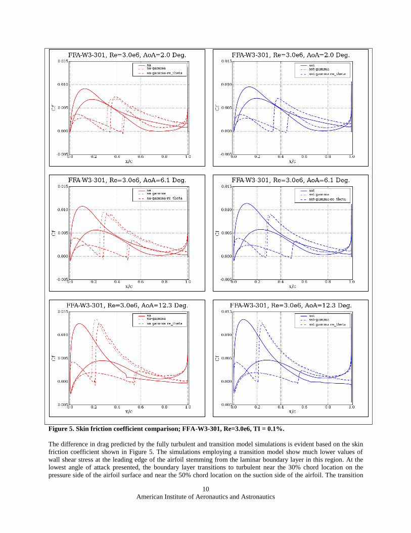
Figure 5. Skin friction coefficient comparison; FFA-W3-301, Re=3.0e6, TI = 0.1%.

The difference in drag predicted by the fully turbulent and transition model simulations is evident based on the skin

friction coefficient shown in Figure 5. The simulations employing a transition model show much lower values of

wall shear stress at the leading edge of the airfoil stemming from the laminar boundary layer in this region. At the

lowest angle of attack presented, the boundary layer transitions to turbulent near the 30% chord location on the

pressure side of the airfoil surface and near the 50% chord location on the suction side of the airfoil. The transition


11

location is characterized by the rapid increase in the skin friction coefficient. As the angle of attack is increased, the

transition location of the suction side boundary layer moves forward, while the transition location of the pressure

side boundary layer moves towards the trailing edge. This change in transition location is a direct result of the

change in pressure gradient that occurs as the angle of attack is increased.

Figure 5 also indicates that the γ-Reθ model tends to predict a later transition location when compared to the γ

model. This trend appears for the Spalart-Allmaras model at all angles of attack presented, and for the SST closure

at 6.1 and 12.3 degree angles of attack. This subtle change in the transition location is clearly evident in the plots of

skin friction coefficient, and also appears in the plots of drag coefficient. The γ-Reθ model tends to predict a slightly

lower drag regardless of which turbulence closure it is paired with.

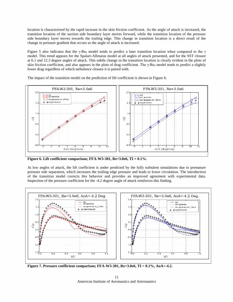
The impact of the transition model on the prediction of lift coefficient is shown in Figure 6.

At low angles of attack, the lift coefficient is under predicted by the fully turbulent simulations due to premature

pressure side separation, which increases the trailing edge pressure and leads to lower circulation. The introduction

of the transition model corrects this behavior and provides an improved agreement with experimental data.

Inspection of the pressure coefficient for the -4.2 degree angle of attack reinforces this finding.

Figure 6. Lift coefficient comparison; FFA-W3-301, Re=3.0e6, TI = 0.1%.

Figure 7. Pressure coefficient comparison; FFA-W3-301, Re=3.0e6, TI = 0.1%, AoA=-4.2.


12

Figure 7 illustrates that the fully turbulent simulations consistently over predict the pressure coefficient along the

trailing edge of the airfoil surface whereas the transition model simulations show closer agreement with experiment

in this region. At higher angles of attack, the pressure coefficient predicted by the transition simulations also shows

consistent improvement over the fully turbulent results. This is illustrated in Figure 8.

Figure 8. Pressure coefficient comparison; FFA-W3-301, Re=3.0e6, TI = 0.1%.


13

With the benefits of transition modeling clearly illustrated, we now turn our attention to a comparison between the

available transition models. Inspection of the lift and drag results from the sa-gamma and sa-gamma-re_theta models

show very little difference between the two transition closures. The simplifications present in the sa-gamma model

appear to have no significant impact on the results of the simulations. The same conclusion is reached when

comparing the sst-gamma model results with the sst-gamma-re_theta results. The differences that appear in terms of

transition location do impact the results, but all results are deemed to match well with experiment.

The next result of interest is an analysis of all 4 transition model combinations in comparison to each other and to

experiment.

Figure 9. Drag polar comparison; FFA-W3-301, Re=3.0e6, TI = 0.1%.

Figure 9 indicates the excellent agreement between all transition models for the FFA-W3-301 airfoil. It also

reinforces the benefits of including transition compared to the fully turbulent results. Analysis of the drag polar also

reveals some additional trends, however. At low angles of attack, the Spalart-Allmaras based transition models

provide a slightly better match with data by predicting a higher drag coefficient when compared against the SST

based models. As the angle of attack increases, we see a slight deviation of the results based on which transition

closure is used. For both the Spalart-Allmaras and SST based models, the γ transition closure shows slightly higher

drag predictions than the γ-Reθ closure does. Although this deviation in behavior exists at the higher angles of

attack, the results of all transition models agree very well with each other and provide improvements in the

comparison to experiment over the fully turbulent results.

In addition to the drag polar, the lift to drag ratio is used as a metric to quantify the performance of the transition

models. This metric is plotted in the following figure.


14

Figure 10. Lift to drag ratio comparisons; FFA-W3-301, Re=3.0e6, TI = 0.1%.

Figure 10 once again reinforces the improvement to the results that is realized when using the transition models. The

fully turbulent cases under predict the lift to drag ratio at all but the lowest angle of attack. All 4 transition model

combinations improve on this result and provide good agreement with experimental data. As the airfoil approaches

stall, however, we do see some deviation between simulation and experiment. This behavior is expected, and is

attributed more to a weakness of the underlying RANS model than a deficiency of the transition model.

Visual inspection of each of the flow field provides further insight into the impact that the transition model has on

the flow around the airfoil. The transition model delays the growth of eddy viscosity in the boundary layer by

suppressing the growth of turbulent kinetic energy until the local conditions are favorable for the generation of

turbulent structures. In the case of the airfoil, the transition process is dominated by the local pressure gradient.

Favorable pressure gradients tend to suppress the growth of the turbulent boundary layer, while an adverse pressure

gradient tends to accelerate the rate at which turbulent kinetic energy increases. The eddy viscosity fields predicted

by each of the models is shown in Figure 11. For the fully turbulent simulations, the eddy viscosity begins to grow at

the leading edge of the airfoil and gives rise to a rapidly thickening boundary layer. The transition model

simulations, however, delay the appearance of the turbulent boundary layer until the flow has reached approximately

40% of the airfoil chord. Visual inspection of the eddy viscosity field also reaffirms the similarities in the results

predicted by the 4 different transition models. At this low angle of attack, there is no discernable difference between

the models.


15

Figure 11. Contours of viscosity ratio for the FFA-W3-301 airfoil simulations; Re=3.0e6, TI=.1%, AoA= 0.0

degrees.

The results of this first set of experimental comparisons shows a very promising trend in the simulations. The

Spalart-Allmaras based transition models agree well with the SST based transition models. In addition, there is

excellent agreement between the γ and γ-Reθ transition models regardless of which turbulence model they are

coupled with. With the level of accuracy established, the next metric of interest is the computational expense

associated with each modeling approach. To provide some insight into this, the total non-linear iteration count

necessary to perform the simulations in the range of -5 to 12 degrees angle of attack was summed for each model.

The performance numbers were then normalized by the fully turbulent Spalart-Allmaras metrics. The relative

number of iterations and relative run time for each modeling approach is summarized in Table 4.

sa sa-gamma sa-gamma-re_theta sst sst-gamma sst-gamma-re_theta

Relative iterations 1.0 1.0 1.04 0.76 1.36 0.92

Relative run time 1.0 0.91 1.80 1.16 1.92 1.45

Table 4. Performance comparison for angles of attack ranging between -5 and 12 degrees.

Table 4 indicates that the increase in non-linear iteration count for the sweep of angles of attack on this airfoil is

very modest. For the case of sst-gamma-re_theta, the transition model simulations take a smaller total number of

iterations than the fully turbulent Spalart-Allmaras model does. This finding is somewhat surprising, but it must be

kept in mind that the expense of the iterations increases when additional equations are added. This expense comes

from the additional complexity of the non-linear system as well as the increase in stiffness of the linear systems that

arise with transition models. When considering the additional expense of the iterations, the only model that produces

solutions in comparable run time as the fully turbulent Spalart-Allmaras model is the sa-gamma model. Although

this is a promising result, these results do not take into account the post-stall behavior of the models. When

including the stall and post-stall angles of attack, we obtain the following performance results:

sa sa-gamma sa-gamma-re_theta sst sst-gamma sst-gamma-re_theta

Relative iterations 1.0 1.25 1.28 0.72 1.66 0.93

Relative run time 1.0 1.24 2.42 1.09 2.44 1.44

Table 5. Performance comparison for angles of attack ranging between -20 and 20 degrees.


16

The performance trend of the models remains consistent in the sense that sa-gamma provides the best performance

relative to the fully turbulent Spalart-Allmaras simulation. When including all angles of attack, however, we see that

the total cost of adding the transition model is on the order of 25%. The additional expense associated with the

transition models is expected to be case dependent, but the metrics shown for this application are extremely

promising, indicating that for pre-stall angles of attack, the additional compute expense of transition is negligible

when using the sa-gamma model.

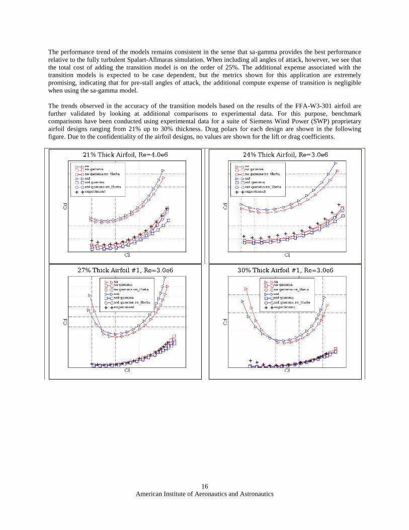
The trends observed in the accuracy of the transition models based on the results of the FFA-W3-301 airfoil are

further validated by looking at additional comparisons to experimental data. For this purpose, benchmark

comparisons have been conducted using experimental data for a suite of Siemens Wind Power (SWP) proprietary

airfoil designs ranging from 21% up to 30% thickness. Drag polars for each design are shown in the following

figure. Due to the confidentiality of the airfoil designs, no values are shown for the lift or drag coefficients.


17

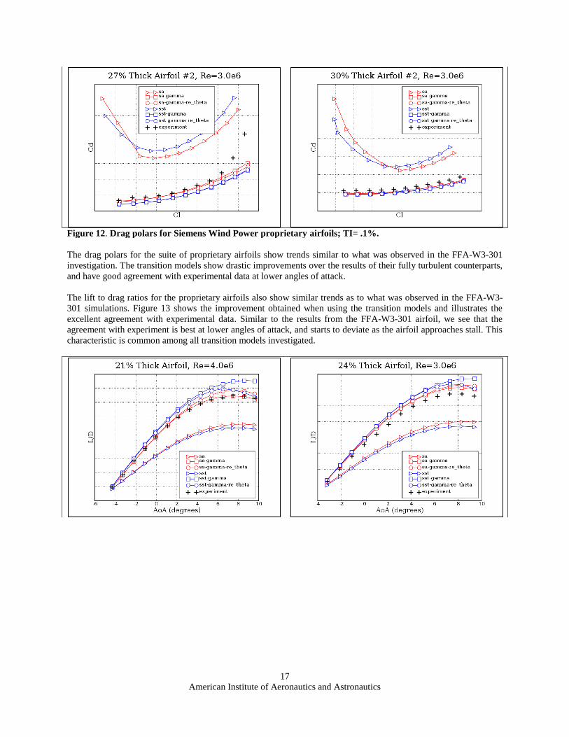
Figure 12. Drag polars for Siemens Wind Power proprietary airfoils; TI= .1%.

The drag polars for the suite of proprietary airfoils show trends similar to what was observed in the FFA-W3-301

investigation. The transition models show drastic improvements over the results of their fully turbulent counterparts,

and have good agreement with experimental data at lower angles of attack.

The lift to drag ratios for the proprietary airfoils also show similar trends as to what was observed in the FFA-W3-

301 simulations. Figure 13 shows the improvement obtained when using the transition models and illustrates the

excellent agreement with experimental data. Similar to the results from the FFA-W3-301 airfoil, we see that the

agreement with experiment is best at lower angles of attack, and starts to deviate as the airfoil approaches stall. This

characteristic is common among all transition models investigated.


18

Figure 13. Lift to drag ratios for Siemens Wind Power proprietary airfoils. TI= .1%.

IV. Wind Turbine Simulations

A. NREL Phase-VI Wind Turbine Rotor

The NREL Phase-VI model-scale rotor is one of the most widely investigated configurations in wind power research

due to the availability of detailed experimental data16. In this work, the NREL model is investigated using the same

suite of models that was applied to the airfoil cases. Of specific interest from the results are the rotor thrust, power,

pressure coefficient, and robustness of the transition closures for application to three-dimensional industrial scale

applications.

B. Geometry Construction

A solid model of the NREL Phase-VI geometry was created based on the S-809 airfoil sections that make up the

blade. This geometry was imported into SolidWorks where the bounding fluid volume around the rotor was created

using a cylindrical solid region. A boolean subtraction operation was used to subtract the blade volume from the

surrounding volume, leaving only the air volume represented as a geometric solid. To keep the computational

expense to a minimum, we exploit the rotational periodicity of the 2-bladed rotor. By modeling a 180-degree sector

of the rotor, only a single blade is modeled, but the aerodynamics of the full rotor are taken into account through the

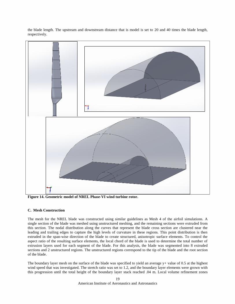
periodic constraints. The geometric model for simulations of the NREL blade is shown in Figure 14. Note that the

blade surface has been segmented along its length to generate geometric edges that will be utilized in the meshing

process. Additionally, the blade is nested within a smaller cylindrical volume, which will be used to form the region

in which the model is solved in a rotating frame of reference. To minimize the impact of any boundary conditions

applied to the CFD model, the outer bounding cylinder of the domain is sized to have a diameter equal to 20 times


19

the blade length. The upstream and downstream distance that is model is set to 20 and 40 times the blade length,

respectively.

Figure 14. Geometric model of NREL Phase-VI wind turbine rotor.

C. Mesh Construction

The mesh for the NREL blade was constructed using similar guidelines as Mesh 4 of the airfoil simulations. A

single section of the blade was meshed using unstructured meshing, and the remaining sections were extruded from

this section. The nodal distribution along the curves that represent the blade cross section are clustered near the

leading and trailing edges to capture the high levels of curvature in these regions. This point distribution is then

extruded in the span-wise direction of the blade to create structured, anisotropic surface elements. To control the

aspect ratio of the resulting surface elements, the local chord of the blade is used to determine the total number of

extrusion layers used for each segment of the blade. For this analysis, the blade was segmented into 8 extruded

sections and 2 unstructured regions. The unstructured regions correspond to the tip of the blade and the root section

of the blade.

The boundary layer mesh on the surface of the blade was specified to yield an average y+ value of 0.5 at the highest

wind speed that was investigated. The stretch ratio was set to 1.2, and the boundary layer elements were grown with

this progression until the total height of the boundary layer stack reached .04 m. Local volume refinement zones


20

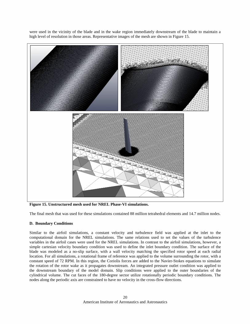
were used in the vicinity of the blade and in the wake region immediately downstream of the blade to maintain a

high level of resolution in those areas. Representative images of the mesh are shown in Figure 15.

Figure 15. Unstructured mesh used for NREL Phase-VI simulations.

The final mesh that was used for these simulations contained 88 million tetrahedral elements and 14.7 million nodes.

D. Boundary Conditions

Similar to the airfoil simulations, a constant velocity and turbulence field was applied at the inlet to the

computational domain for the NREL simulations. The same relations used to set the values of the turbulence

variables in the airfoil cases were used for the NREL simulations. In contrast to the airfoil simulations, however, a

simple cartesian velocity boundary condition was used to define the inlet boundary condition. The surface of the

blade was modeled as a no-slip surface, with a wall velocity matching the specified rotor speed at each radial

location. For all simulations, a rotational frame of reference was applied to the volume surrounding the rotor, with a

constant speed of 72 RPM. In this region, the Coriolis forces are added to the Navier-Stokes equations to simulate

the rotation of the rotor wake as it propagates downstream. An integrated pressure outlet condition was applied to

the downstream boundary of the model domain. Slip conditions were applied to the outer boundaries of the

cylindrical volume. The cut faces of the 180-degree sector utilize rotationally periodic boundary conditions. The

nodes along the periodic axis are constrained to have no velocity in the cross-flow directions.


21

E. Comparison Against Experimental Data

The NREL rotor simulations were run using all 6 turbulence/transition model combinations at wind speeds

corresponding to 5, 7, 10, 13, 15, 20, and 25 m/s. Each case was iterated to convergence using the same solution

strategy as identified for the airfoil simulations. The thrust and power of the rotor was monitored during the

simulations to identify the level to which the forces on the blade had converged. Due to the challenge in obtaining a

completely steady solution at all wind speeds for this application, the convergence was monitored by comparing the

agreement between the average forces on the blades. For lower wind speeds that converge readily to a steady

solution, the simulations were halted when the instantaneous forces agreed within .1% of the averaged forces from

the last 20 time steps. However, at higher wind speeds, low amplitude oscillations in the solution prevented these

criteria from ever being met. Therefore, a second averaging window was defined and the results from a short and

long time averaging window were compared to determine force convergence. This method detects a solution that is

oscillating about a mean value that is not drifting in time. For wind speeds around the stall point of the rotor, these

criteria were responsible for halting the simulation. Using this approach, convergence was deemed sufficient when

the total change in forces on the blade differed by no more than .1% over averaging windows of 20 steps and 40

steps.

The thrust and power from each of the simulations is shown in Figure 16.

Figure 16. Thrust and power prediction for the NREL Phase-VI rotor.

Review of Figure 16 indicates a number of trends in the results. The first trend of interest is the relative insensitivity

of the thrust to the modeling approach that is employed. For the Spalart-Allmaras based simulations, there is very

little change in the predicted thrust when comparing fully turbulent and transition model results. The SST based

simulations show a small amount of sensitivity in the thrust results near stall (i.e. 10 m/s wind speed). Although the

difference is minor, the SST-gamma-re_theta model predicts slightly lower values of thrust, which does produce a

better agreement with test data.

Analysis of the power predictions shows a much different trend in comparison to the thrust. The power values vary

significantly between the turbulence closures as well as the transition closures, but there are some consistent trends

that are observed. The first observation is that the fully turbulent simulations under predict the rotor power at the 5

m/s and 7 m/s wind speed. Inclusion of the effects of transition increase the predicted power at these wind speeds

and yields good agreement with the test data. This trend holds true for both the Spalart-Allmaras and SST based

models, implying that the transition models are delaying the growth of the turbulent boundary layer appropriately.

As the rotor approaches stall at the 10 m/s wind speed, the differences in the models appear more clearly. The

Spalart-Allmaras based models all over predict the power due to an over prediction of lift along the blade. The SST

based models show a similar level of over prediction for the fully turbulent case and for the sst-gamma case, but the

sst-gamma-re_theta model is doing a much better job at predicting the stall. Investigation of the pressure coefficient

along the blade reveals the cause for the differences in predicted power.


22

Figure 17. Pressure coefficients on NREL Phase-VI turbine blade for the 10 m/s wind speed.

The pressure coefficients reveal the difference in behavior between the models. The inboard section of the blade (i.e.

30% radial location) is predicted with a similar level of accuracy by all models. The models are also comparing well

to the experimental data at this location. However, at the 47% radial location, the models differ significantly, and all

but the sst-gamma-re_theta model over predict the lift. The sst-gamma-re_theta model shows less of a suction peak,

indicating the onset of stall, and leads to the better prediction of rotor power. Although none of the models match the

experimental data for the inboard sections, the sst-gamma-re_theta model shows the best agreement. Comparing

results further out towards the tip of the blade indicates the opposite trend. At the 63% radial location, the sst-

gamma-re_theta model indicates leading edge stall whereas the other models reproduce the leading edge suction

peak that is present in the experimental data. As the results are compared to experiment further out along the blades,

the agreement between models returns and the comparison to experiment is favorable.


23

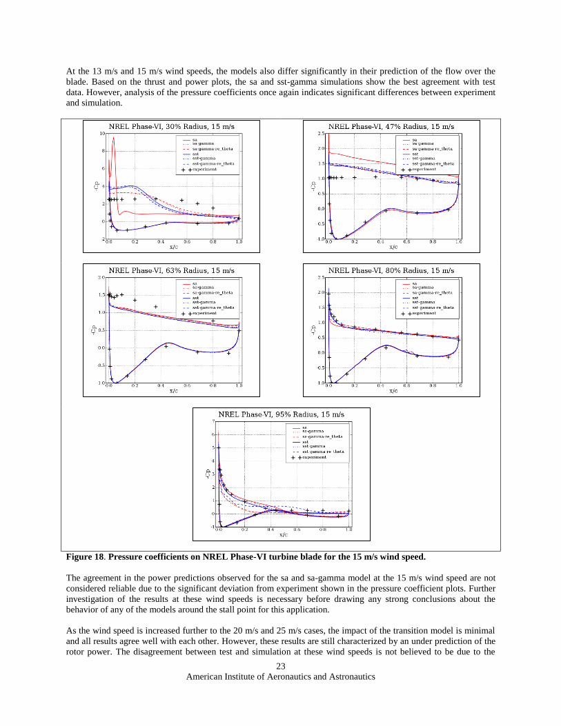
At the 13 m/s and 15 m/s wind speeds, the models also differ significantly in their prediction of the flow over the

blade. Based on the thrust and power plots, the sa and sst-gamma simulations show the best agreement with test

data. However, analysis of the pressure coefficients once again indicates significant differences between experiment

and simulation.

Figure 18. Pressure coefficients on NREL Phase-VI turbine blade for the 15 m/s wind speed.

The agreement in the power predictions observed for the sa and sa-gamma model at the 15 m/s wind speed are not

considered reliable due to the significant deviation from experiment shown in the pressure coefficient plots. Further

investigation of the results at these wind speeds is necessary before drawing any strong conclusions about the

behavior of any of the models around the stall point for this application.

As the wind speed is increased further to the 20 m/s and 25 m/s cases, the impact of the transition model is minimal

and all results agree well with each other. However, these results are still characterized by an under prediction of the

rotor power. The disagreement between test and simulation at these wind speeds is not believed to be due to the


24

impact of boundary layer transition, and the agreement of the fully turbulent simulations with the transition model

cases supports this theory.

The agreement with test data for the NREL Phase-VI model is improved by the introduction of the transition models

at the lower wind speeds. As the wind speed is increased and the rotor approaches stall, the influence of the

transition models becomes less consistent. Review of the available data indicates that in some cases where the

integrated quantities (i.e. rotor power) are improved by the transition model, the local quantities are not necessarily

improved (i.e. pressure coefficient). Although the sst-gamma-re_theta model shows good agreement with test for the

rotor power at 10 m/s, review of the pressure coefficient indicates significant error when compared to test data. This

same argument applies to the performance of the sst-gamma model at the 15 m/s wind speed.

V. Summary

In this work, a series of simulations relevant to wind power engineering were performed for the purpose of assessing

the performance of local correlation-based transition models. The investigation focused on the γ-Reθ and γ transition

closures paired with the Spalart-Allmaras and SST turbulence models. The performance of the transition models, as

well as their fully turbulent counter parts, were compared on a series of 7 different airfoil designs and the NREL

Phase-VI wind turbine rotor.

The findings from the airfoil simulations illustrate the benefit of incorporating the transition model closures into the

simulations. Fully turbulent simulations using both the Spalart-Allmaras and SST turbulence models show a

consistent over prediction of drag when comparing against experimental data. Introduction of a transition model into

the simulation improved the prediction of drag regardless of the underlying RANS model that was in use. This

improvement to predictive capability appears in the pre-stall regime. As the airfoils approach stall, the physics

become increasingly difficult for the underlying RANS model to capture properly, and the benefits of including a

transition model diminish, regardless of which model combination is employed.

The airfoil simulations were also successful at illustrating the agreement in predictive capability between the γ-Reθ

and γ transition closures when paired with a given RANS model. Both transition closures show similar trends and

exhibit similar levels of accuracy. Although all transition/turbulence model combinations produced substantial

improvement over fully turbulent simulations, the Spalart-Allmaras based transition simulations showed slightly

better agreement with experiment.

When comparing the expense of the various modeling approaches, the Spalart-Allmaras based closures have some

clear advantages. The mesh sensitivity study illustrated the relaxed meshing requirements that the Spalart-Allmaras

model has in comparison to the SST model. The Spalart-Allmaras model appears to achieve grid convergence using

approximately 130,000 nodes whereas it was necessary to use nearly double that node count to achieve grid

convergence using the SST model. This sensitivity is evident for both fully turbulent simulations as well as cases

that utilize a transition model. In addition to the increased meshing expense, the overall run time of the simulations

using the SST based models was shown to be greater than the Spalart-Allmaras based equivalents. When

investigating the pre-stall performance of the FFA-W3-301 airfoil, the total compute time of the sa-gamma model

was equivalent to the fully turbulent Spalart-Allmaras simulation. This illustrates the efficiency of the single

equation RANS closure coupled with the single equation transition model.

The suite of transition models was also applied to simulations of the NREL Phase-VI wind turbine rotor. These

simulations revealed trends that were consistent with the findings of the airfoil simulations. At pre-stall wind speeds,

the introduction of a transition model consistently improved the prediction of rotor power when compared to fully

turbulent simulations. This trend was observed for both the Spalart-Allmaras and SST models when paired with the

γ and γ-Reθ transition models. As the wind speed increases, the rotor approaches stall, and differences appeared

based on which RANS closure and transition model was in use. The sst-gamma-re_theta model proved to be the

only model that predicted the stalled portions of the blade at the 10 m/s wind speed. This model combination also

did the best job at predicting power at the 13 m/s wind speeds. At 15 m/s, however, it over predicted the stall and

thus under predicted the power output of the rotor. This observation further reinforces the inability of transition

closures to improve RANS predictions of flows near or at stall.


25

The benefits of using transition models to simulate applications relevant to wind turbine blade design are clearly

illustrated by the results presented in this work. The γ-Reθ and γ models show similar levels of accuracy in the pre-

stall regime. These models also show similar levels of accuracy when paired with either the Spalart-Allmaras or SST

RANS closure. With these findings, it is concluded that all models are suitable for application in wind power

engineering, and engineers can freely choose from the available suite to fit their needs. Due to the relaxed meshing

requirements and reduced set of differential equations, however, the sa-gamma model provides clear performance

benefits over the others and incorporates the effect of transition for very little additional compute cost when

compared to fully turbulent simulations.

Acknowledgements

D. Corson wishes to thank Siemens Wind Power for the use of their test data and also for their guidance throughout

this investigation. Their input has been an invaluable contribution to this work.

References

1 Langtry, R.B., Menter, F.R.,2009, “Correlation-Based Transition Modeling for Unstructured Parallelized

Computational Fluid Dynamics Codes”. AIAA J. 47(12), 2984-2906 2 Menter, F.R., Smirnov, P.E., Liu, T., Avancha, R.,2015, “A One-Equation Local Correlation-Based Transition

Model”, Flow, Turbulence, and Combustion. 1-37 3 Medida,S., Baeder, J.,2011, “Application of the Correlation-based γ-Reθ Transition Model to the Spalart-

Allmaras Turbulence Model”, AIAA 201103979, 20th AIAA Computational Fluid Dynamics Conference, Honolulu,

Hawaii. 4 Medida, S., Corson, D., Barton, M., 2016, “Implementation and Validation of Correlation-based Transition

Models in AcuSolve”, AIAA Aviation Conference, Washington DC, June 13-17. 5 Hughes, T.J.R., Franca, L.P. and Hulbert, G.M., 1989, "A new finite element formulation for computational

fluid dynamics.VIII. The Galerkin/least-squares method for advective-diffusive equations", Comp. Meth. Appl.

Mech. Engg., 73, pp 173-189. 6 Shakib, F., Hughes, T.J.R. and Johan, Z., 1991, "A new finite element formulation for computational fluid

dynamics. X. The compressible Euler and Navier-Stokes equations", Comp. Meth. Appl. Mech. Engg., 89, pp 141-

219. 7 Godo, M.N, Corson, D. and Legensky, S.M., 2009, “An Aerodynamic Study of Bicycle Wheel Performance

using CFD”, 47th AIAA Aerospace Sciences Annual Meeting, Orlando, FL, USA, 5-8 January, AIAA Paper No.

2009-0322. 8 Lyons, D.C., Peltier, L.J., Zajaczkowski, F.J., and Paterson, E.G., 2009 “Assessment of DES Models for

Separated Flow From a Hump in a Turbulent Boundary Layer”, J. Fluids Engg, 131, 111203-1 – 111203-9. 9 Bagwell, T.G., “CFD Simulation fo Flow Tones From Grazing Flow Past a Deep Cavity”, Proceedings of 2006

ASME International Mechanical Engineering Congress and Exposition, Nov. 5-10, 2006, Chicago, Illinois. 10 Johnson, K and Bittorf, K., “Validating the Galerkin Least Square Finite Element Methods in Predicting

Mixing Flows in Stirred Tank Reactors”, Proceedings of CFD 2002, The 10th Annual Conference of the CFD

Society of Canada, 2002. 11Corson, D. A., Griffith, D. T., Ashwill, T., and Shakib, F., 2012, “Investigating aeroelastic performance of

multi-megawatt wind turbine rotors using CFD”, AIAA 2012-1827, 53rd AIAA/ASME/ASCE/AHS/ASC Structures,

Structural Dynamics and Materials Conference. 12 Jansen, K. E. , Whiting, C. H. and Hulbert, G. M., 2000, "A generalized-alpha method for integrating the

filtered Navier-Stokes equations with a stabilized finite element method", Comp. Meth. Appl. Mech. Engg.", 190, pp

305-319. 13 Spalart, P.R. and Allmaras, S.R., 1992, “A one-equation Turbulence Model for Aerodynamic Flows”, 30th

AIAA Aerospace Sciences Annual Meeting, Reno NV, USA, 6-9 January, AIAA Paper No. 92-0439. 14 Menter, F.R.,1994, Two-equation eddy-viscosity turbulence models for engineering applications. AIAA J.

32(8), 269-289 15Bjork, A., 1990, “Coordinates and Calculation for the FFA-Wl-xxx, FFA-W2-x.u, FFA-W3-xxx Series of

Airfoils for Horizontal Axis Wind Turbines”, The Aeronautical Research Institute of Sweden, Technical Report

FFA TN 1990-15.


26

16Fuglsang, P., Antoniou, I., Dahl, K., Madsen, H., 1998, “Wind Tunnel Tests of the FFA-W3-241, FFA-W3-

301, and NACA 63-430 Airfoils,” Riso Tech. Report Riso-R-1041(EN).

17Hand, M. M., Simms, D. A., Fingersh, L. J., Jager, D. W., Cotrell, J. R., Schrech, S., Lawood, S. M., 2001,

“Unsteady aerodynamics experiment phase VI: Wind tunnel test configurations and available data campaigns,”

NREL Tech. Report TP-500-29955.

a comparative assessment of correlation-based transition ... · pdf filea comparative...

Documents