a compact high-brightness liquid-metal-jet x-ray source10352/... · 2006-05-30 · the first x-ray...
TRANSCRIPT

A Compact High-Brightness Liquid-Metal-Jet X-Ray Source
Mikael Otendal
Doctoral Thesis Department of Applied Physics Royal Institute of Technology
Stockholm, Sweden 2006

TRITA-FYS 2006:36 ISSN 0280-316X ISRN KTH/FYS/--06:36--SE ISBN 91-7178-371-7 Akademisk avhandling som med tillstånd av Kungl. Tekniska Högskolan framlägges till offentlig granskning för avläggande av teknologie doktorsexamen fredagen den 9 juni 2006 klockan 10.00 i seminariesal D3, Lindstedtsvägen 5, Kungl. Tekniska Högskolan, Stockholm.
© Mikael Otendal, maj 2006
Tryck: Universitetsservice US AB


iii
To my family
”Listen, damn it, we will win”
James Hetfield


v
Abstract
This thesis describes the development and characterization of a compact high-brightness liquid-metal-jet anode x-ray source. Initial calculations show that a source based on this concept could potentially lead to a >100-fold increase of the brightness compared to current state-of-the-art rotating-anode x-ray sources. This improvement is due to an increased thermal load capacity of the anode.
A low-power proof-of-principle source has been built, and experiments show that the liquid-metal-jet anode can be operated at more than an order of magnitude higher power densities than modern solid-metal anodes. This brightness enhancement has been utilized to acquire in-line phase-contrast images of weakly absorbing objects with substantially shorter exposure times than previously reported. To be able to target different application areas different liquid-jet-anode materials have been tested. The Sn-jet anode could potentially be used in mammography examinations, whereas the Ga-jet could be utilized for, e.g., protein-structure determination with x-ray diffraction.
Scaling to higher power and brightness levels is discussed and seems conceivable. A potential obstacle for further development of this source concept, the generation of a microscopic high-speed liquid-metal jet in vacuum, is investigated and is proven to be feasible. Dynamic-similarity experiments using water jets to simulate 30-µm, ~500-m/s tin and gallium jets show good coherence and directional stability of the jet. Other potential difficulties in the further source development, such as excessive debris emission and instabilities of the x-ray emission spot, are also investigated in some detail.


vii
List of Papers
This thesis is based on the following papers:
Paper 1 O. Hemberg, M. Otendal, and H. M. Hertz, “Liquid-Metal-Jet Anode Electron-Impact X-Ray Source”, Appl. Phys. Lett. 83, 1483-1485 (2003).
Paper 2 O. Hemberg, M. Otendal, and H. M. Hertz, “A Liquid-Metal-Jet Anode X-Ray Tube”, Opt. Eng. 43, 1682-1688 (2004).
Paper 3 M. Otendal, O. Hemberg, T. T. Tuohimaa, and H. M. Hertz, “Microscopic High-Speed Liquid-Metal Jets in Vacuum”, Exp. Fluids 39, 799-804 (2005).
Paper 4 T. Tuohimaa, M. Otendal, and H. M. Hertz, “X-Ray Imaging with an Electron-Impact Liquid-Metal-Jet-Anode Source”, submitted to Radiology.
Paper 5 M. Otendal, T. Tuohimaa, and H. M. Hertz, “Stability and Debris in Liquid-Metal-Jet-Anode Microfocus X-Ray Sources”, submitted to J. Appl. Phys.
Paper 6 M. Otendal, T. Tuohimaa, U. Vogt, and H. M. Hertz, “A 9-keV Electron-Impact Liquid-Gallium-Jet X-Ray Source”, submitted to Appl. Phys. Lett.

ix
Other Publications
The following papers, contributed to by the author, are related to the work in this thesis, but are not included in it.
Papers O. Hemberg, M. Otendal, and H. M. Hertz, “The Liquid-Metal-Jet Anode X-Ray Source”, Proc. SPIE 5196, 421-431 (2003).
P. A. C. Jansson, B. A. M. Hansson, O. Hemberg, M. Otendal, A. Holmberg, J. de Groot, and H. M. Hertz, “Liquid-Tin-Jet Laser-Plasma Extreme Ultraviolet Generation”, Appl. Phys. Lett. 84, 2256-2258 (2004).
M. Otendal, T. Tuohimaa, O. Hemberg, and H. M. Hertz, “Status of the Liquid-Metal-Jet Anode Electron-Impact X-Ray Source”, Proc. SPIE 5537, 57-63 (2004).
T. Tuohimaa, M. Otendal, and H. M. Hertz, “High-Intensity Electron Beam for Liquid-Metal-Jet Anode Hard X-Ray Generation”, Proc. SPIE 5918, 225-230 (2005).


xi
Contents
Abstract ....................................................................................................................... v List of Papers ............................................................................................................ vii Other Publications ..................................................................................................... ix Contents ..................................................................................................................... xi Chapter 1 Introduction.................................................................................................1 Chapter 2 Liquid Jets .................................................................................................. 3
2.1 Physical Breakup Mechanisms of Liquid Jets.................................................................. 3 2.1.1 Surface Tension........................................................................................................ 3 2.1.2 Viscosity .................................................................................................................... 5 2.1.3 Atmospheric Interactions ....................................................................................... 5 2.1.4 Velocity Profile Relaxation ..................................................................................... 6 2.1.5 Turbulence ................................................................................................................ 8
2.2 Jet Characterization in Practice ......................................................................................... 8 2.2.1 Reynolds Number.................................................................................................... 9 2.2.2 Weber Number ........................................................................................................ 9 2.2.3 Atmospheric Weber Number............................................................................... 10 2.2.4 Mach Number ........................................................................................................ 10 2.2.5 Ohnesorge Number............................................................................................... 11 2.2.6 Stability Curve ........................................................................................................ 11
2.3 Jet Velocity and Nozzle Design ...................................................................................... 12 2.4 Liquid Jets in Vacuum ...................................................................................................... 14
2.4.1 Cavitation ................................................................................................................ 14 2.4.2 High-Speed Liquid-Metal Jets in Vacuum.......................................................... 15
Chapter 3 Introductory X-Ray Physics......................................................................17 3.1 Electron-Matter Interaction............................................................................................. 17
3.1.1 Atomic Configuration ........................................................................................... 18 3.1.2 Electron Attenuation and Backscattering ........................................................... 18 3.1.3 Continuous Bremsstrahlung ................................................................................. 19 3.1.4 Characteristic Line Emission and Auger Electrons........................................... 20
3.2 X-Ray-Matter Interaction................................................................................................. 22 3.2.1 Photoelectric Absorption...................................................................................... 22 3.2.2 Scattering................................................................................................................. 23
3.3 Index of Refraction........................................................................................................... 24
xii Contents
Chapter 4 Electron-Impact X-Ray Sources ..............................................................27 4.1 Conventional Electron-Impact Sources .........................................................................28
4.1.1 Stationary-Anode Tubes........................................................................................28 4.1.2 Rotating-Anode Tubes ..........................................................................................29
4.2 Liquid-Metal-Jet Anode X-Ray Source...........................................................................32 4.2.1 Source Principles ....................................................................................................32 4.2.2 Performance Characteristics and Future Improvements ..................................33
Chapter 5 X-Ray Imaging .........................................................................................35 5.1 Absorption-Contrast Imaging..........................................................................................36 5.2 Phase-Contrast Imaging....................................................................................................38
5.2.1 X-Ray Interferometry ............................................................................................39 5.2.2 Diffraction-Enhanced Imaging ............................................................................40 5.2.3 In-Line Phase-Contrast Imaging ..........................................................................42
Appendix....................................................................................................................47 Summary of Papers....................................................................................................49 Acknowledgements ................................................................................................... 51 Bibliography ..............................................................................................................53

1
Chapter 1
Introduction
Almost instantly after their discovery in 1895 [1], x-rays found extensive use in science, industry, and medicine. This is still the case today, and that is due to some basic properties of x-rays, such as their ability to penetrate optically opaque objects and, thus, reveal otherwise hidden information about internal structures and material properties. Other important factors for the wide acceptance and exploitation of Röntgen’s discovery was the rather simple equipment required to both produce and detect this new kind of radiation. This made it possible to immediately set up a variety of different experiments, e.g., imaging of the human interior (cf. Fig. 1.1 below), as well as basic materials research.
Figure 1.1. The first x-ray image (Mrs. Röntgen’s hand, 1895).
In the early years, the development of x-ray imaging was mainly in the area of source improvements. In 1919 the line focus principle was discovered, and about a decade later, in 1929, the idea of having a rotating anode was realized. However, since then there have been no further breakthroughs in terms of source performance, but rather gradual improvements mostly due to refined engineering of the x-ray tube. With the advent of modern electronics in the 1960s, substantial progress in the field of image acquisition, and digital image processing and storage took place. Therefore, most modern applications are

2 Chapter 1. Introduction
limited by the source performance, which motivates further development and improvement of x-ray sources.
This thesis is about a novel source concept where x-rays are emitted when a beam of energetic electrons interact with a liquid-metal-jet anode. This is a kind of electron-impact source, just like most modern x-ray tubes, but this particular source can reach higher brightness values than conventional compact sources. Brightness is the radiated power per unit source area and unit solid angle, and since this quantity cannot be increased, but at best conserved, in an optical system [2], the maximum obtainable brightness is given by the source brightness.
Utilizing this new source concept, the brightness could possibly be increased by a factor of >100, which would lead to significantly improved imaging possibilities. However, this requires that a stable, fast, and coherent liquid-metal jet can be produced, which will be discussed in some detail in Chapter 2. A brief overview of some basic x-ray physics in given in Chapter 3, whereas modern electron-impact x-ray tubes are compared with this x-ray source based on a liquid-metal-jet anode in Chapter 4. Finally, Chapter 5 is devoted to a description of some possible imaging techniques for acquisition of different types of object information.
3
Chapter 2
Liquid Jets
One of the most critical components in this new type of x-ray source is the high-speed liquid-metal jet. To be able to build a system that can produce such jets a solid understanding of the dynamics of the behavior of fast jets is required. This chapter will therefore briefly present some of the fundamental processes determining the characteristics of the breakup of a liquid jet. To start with, there will be a brief review of the development of the theoretical models describing jet-breakup behavior. Over the years, this has lead to an increased agreement with the actual experiments. However, due to the complexity of the more detailed and general models the results may be difficult to use in practice, which has lead to simpler rules and formulas based on experimental findings for specific types of jets. This approach utilizing more hands-on dimensionless flow parameters will also be discussed in this chapter.
2.1 Physical Breakup Mechanisms of Liquid Jets Liquid jets are inherently unstable. The phenomenon of jet disintegration has been a subject of theoretical and experimental investigations since the early parts of the 1800s [3,4], and over the years it has been ranging in applications from fire hose nozzles to production of metal powder. There are several different physical mechanisms that affect the fashion of which jets break up into droplets. A few of these are discussed in the following subsections, but even though they are treated separately, a real jet is, to some extent, subject to all of these mechanisms simultaneously.
2.1.1 Surface Tension
In 1873, Plateau [5] found that the surface energy of a jet is not the lowest possible if the jet length exceeds its circumference. Instead, it could attain a lower and more stable energetic state if the jet was broken up into droplets. A few years later, Rayleigh [6] presented a mathematical analysis on the instability of jets, where he used a model of an infinite stationary cylinder, consisting of an inviscid incompressible liquid not subjected to gravitational forces. He also superimposed a spectrum of infinitesimal perturbations to the cylinder, but where the jet is only destroyed by the particular disturbance with the spatial frequency with the highest growth rate. By taking the z-axis along the axis of the jet, the radius, r, of the jet would at any time, t, be represented by
4 Chapter 2. Liquid Jets
= + cos r a δ kz , (2.1)
where a is the undisturbed radius of the jet, and δ is the amplitude of the disturbance responsible for the breakup. This amplitude is always small in comparison with a, and k = 2π/λ, where λ is the wavelength of the disturbance. The surface tension forces act for a reduction of the surface energy, which in this case merely is a question of minimizing the surface area of the jet. Calculating the difference in surface area per unit length of the jet for the disturbed (S) and the undisturbed (S0) case results in
( )− = −2
2 20
π 12δS S k aa
. (2.2)
Obviously, ka < 1 results in a decrease of surface area for the disturbed jet, which means that the jet is unstable with respect to the perturbations where λ > 2πa. Given this restriction of λ, Rayleigh further computed the growth rate of the disturbances
( )( ) ( )= −12 2
30
1I γσq γ γI γρa
, (2.3)
where γ = ka, σ and ρ are the surface tension and density of the jet liquid, respectively, and I0 and I1 are zero and first order modified Bessel functions of the first kind. By differentiation and maximization of Eq. 2.3, and assuming exponential growth of the jet perturbations, Rayleigh further developed the expression of the growth rate. The resulting formula was found to be
= 30.97 σqρd
, (2.4)
and is based on the assumption that the amplitude of the disturbance grows exponentially with time and, thus, distance from the nozzle. In the above equation σ and ρ are the surface tension and density of the jet liquid, respectively, and d = 2a is the undisturbed diameter of the jet. By knowing the expression for the disturbance growth rate the formula for calculating the jet breakup length, L, is as follows:
⎛ ⎞= ⎜ ⎟⎝ ⎠
3
01.03 ln
2ρddL v
δ σ, (2.5)
where v is the speed of the jet and δ0 is the initial amplitude of the disturbance. Eq. 2.5 is a result of a linearized analysis of the growth rate of infinitesimal perturbations of the jet, which is only valid if they are small in comparison with the jet radius. But, since a breakup

2.1. Physical Breakup Mechanisms of Liquid Jets 5
is defined as the disturbance growing to the size of the radius, this approach to find the breakup length is not strictly correct. However, for being an initial theoretical investigation, the errors introduced by the linear analysis are not of any major concern, especially not since δ will only become comparable to a close to the breakup point due to its exponential growth.
2.1.2 Viscosity
Weber [7] extended the theory in Section 2.1.1 to include viscous effects of the jet, as well as the interaction of the jet with an inviscid ambient atmosphere. The main contribution of Weber’s work to the understanding of jet disintegration was on how viscosity affects breakup. By adding viscosity to the stationary jet, the expression for the growth rate factor of Eq. 2.4 is modified into
−
⎡ ⎤= +⎢ ⎥⎢ ⎥⎣ ⎦
13 3ρd µdqσ σ
, (2.6)
where µ is the dynamic viscosity, which is commonly referred to as the (coefficient of) viscosity. The breakup length of a viscous jet could be predicted by using Eq. 2.6 instead of Eq. 2.4 as the description of the growth rate, which results in
⎡ ⎤⎛ ⎞= +⎢ ⎥⎜ ⎟
⎝ ⎠ ⎢ ⎥⎣ ⎦
3
0
3ln
2ρd µddL v
δ σ σ. (2.7)
By examining the above expression we see that the viscous effects will always work for increased stability of the jet. In the limit of infinite viscosity, the jet will never break up. The equations above are based on the assumption that the liquid under consideration is Newtonian, i.e., it has a viscosity that is dependent on temperature, but independent of the applied shear rate. Many common real liquids, such as water and molten metals, behave as Newtonian fluids over a wide range of conditions, and it is therefore not a very strict restraint for the jets of interest in this thesis. More information about the viscous behavior of fluids could be found in most standard textbooks on fluid mechanics, e.g., Refs. 8 and 9.
2.1.3 Atmospheric Interactions
As the jet exits from the nozzle, the initial disturbances could be amplified by an ambient atmosphere, which leads to an increased disturbance growth rate. As these growth rate enhancements become significant, Eq. 2.7 will overestimate the breakup length for a viscous jet injected into a non-vacuum atmosphere. The interaction of the jet and the

6 Chapter 2. Liquid Jets
atmosphere could be divided into two subcategories: aerodynamic pressure effects and effects due to the viscosity of the atmosphere.
In the second part of his famous work from 1931, Weber [7] considered the effects of aerodynamic interaction on jet stability, however neglecting the viscosity of the atmosphere. Later, another approach to the problem, this time including the viscosity of the ambient fluid into the equation, was done by Sterling and Sleicher [10]. In their semi-empirical investigation of the interaction of the atmosphere with the jet they found that Weber’s theory did not correctly predict the aerodynamic pressure effect on the breakup process. Based on experimental results they modified Weber’s expression for the growth rate factor q by inserting a scaling factor C to the last term (as seen in Eq. 2.8 below), responsible for atmosphere-related instabilities, i.e.,
( ) ( )( )+ = − +
2 302 2 2
2 3 21
31
2 2Aµγ ρ vγ K γσq q γ γ Cρ K γρa ρa a
. (2.8)
Here, ρA is the density of the atmosphere, K0(γ) and K1(γ) are the zero and first order modified Bessel functions of the second kind, γ is a function of the density of the atmosphere and the viscosity of the jet, and the value of C is 0.175. This theory predicts a maximum of the jet breakup length as the instabilities related to atmospheric interactions become more important for higher jet speeds. The longest breakup length occurs at the so called critical velocity, usually denoted vc, see also Sect. 2.2.6.
These results are strictly valid only for jets where the velocity is constant over the entire cross-section of the jet, i.e., for uniform velocity profiles. Any other velocity profile will, after exit from the nozzle, redistribute to a uniform profile causing destabilization. This phenomenon is more extensively discussed in the next section.
2.1.4 Velocity Profile Relaxation
Many experimental investigations, e.g. [11-13], have failed to verify the formulas in the previous sections, since the effects of the radial flow velocity gradients have not been taken into account. These effects originate from the fact that for a flow of any viscous fluid (µ ≠ 0) in contact with a rigid body, e.g., the interior wall of a nozzle, a boundary layer will be created, where a smooth adjustment of the flow velocity to virtually zero on the boundary of the body takes place [8], cf. Fig. 2.1. This is also known as the no-slip condition.

2.1. Physical Breakup Mechanisms of Liquid Jets 7
Free stream,
v(x)
Boundary
layer, v(x,y)
x
y
Figure 2.1. The flow velocity decreases with the distance to the wall within the boundary layer. Adapted from [14].
The thickness of the boundary layer is a function of the downstream distance – the further downstream, the thicker the boundary layer. Consider a flow in a pipe of infinite length; at a certain point downstream, the entire cross-section of the flow will be made up of a boundary layer. From this point on there will be no change in the velocity profile, hence the flow is referred to as fully developed. Depending on whether the flow is laminar or turbulent the fully developed velocity profile will be different [15-17], see Fig. 2.2.
a)
b)
Figure 2.2. Velocity distributions and flow profiles for a) laminar and b) turbulent flow. Adapted from [18].
As the flow reaches the nozzle exit, the constraint of the nozzle wall is removed and velocity profile relaxation occurs. In this process the velocity components of the jet relaxes into a uniform profile over the entire cross-section, by a mechanism of momentum transfer between transverse layers within the jet [17,19]. The effect of the relaxation depends on the extent to which the velocity profile differs from a uniform profile [10]. As
8 Chapter 2. Liquid Jets
can be seen in Fig. 2.2, a fully developed turbulent flow has a flatter velocity distribution over the jet cross section than the laminar flow profile. This means that, from a velocity profile relaxation point-of-view, fully developed laminar jets are the most unstable upon exit from the nozzle, since the energy redistribution during profile relaxation can be quite violent [17].
2.1.5 Turbulence
When the liquid elements of a jet are flowing in streams parallel to each other and the jet axis, the flow is said to be laminar. When the paths of the liquid particles cross each other in a more or less disorderly manner, the flow is turbulent. Despite the frequent occurrence and technical importance of turbulent flows, e.g., streams from fire hoses and fuel injection in car engines, there is little understanding of the correlation of jet-breakup behavior and turbulence. Due to the high level of complexity of turbulent flows it is very difficult to develop a mathematical theory for the breakup. Instead, much of the knowledge and the vast majority of existing equations describing turbulent jets stem from experimental observations and measurements of jet lengths, drop formation, and drop size distributions.
Experiments have shown that the disturbance at the nozzle exit is considerably larger for fully turbulent jets than for laminar ones [20], thus resulting in a faster breakup. The radial velocity components cause large-amplitude disturbances of the jet at the nozzle exit, creating short wavelength surface waves, soon leading to surface film rupture and the subsequent disintegration of the jet [15]. In combination with atmospheric interactions, turbulent jets will burst into small droplets quickly and violently. It should, however, be noted that the atmosphere is not needed for breakup. Even in a vacuum environment a jet will break up, solely under the influence of its own turbulence [15,21].
2.2 Jet Characterization in Practice Often the level of complexity of a fluid mechanics problem is too high for it to be satisfactorily described mathematically, or the equations describing it cannot be solved. However, methods of using dimensionless flow parameters for describing a flow have been created, and the flows have been empirically categorized depending on their behavior in a certain parameter range. For a more detailed report of the practical use of dimensionless parameters in different flow situations, consult, e.g., Refs. 22-25.
By definition, a dimensionless parameter is the ratio of two similar physical quantities. The analysis of a particular flow problem may be simplified by forming relevant dimensionless parameters, since the number of variables could be reduced [26-28]. Furthermore, these parameters are useful when defining the physical conditions that exist in a flow, and are also good indicators of which properties of a flow that are of importance. The first
2.2. Jet Characterization in Practice 9
technique of using dimensionless parameters to describe a flow system was developed in the early years of the 20th century, and is known as the Buckingham π method [29,30].
In the design process of, e.g., a vessel, an airplane, or a liquid jet, it is very important to know the flow pattern around the structure and the magnitude of the forces acting on the body (or nozzle). To save time and money, and reduce the risk of bad design decisions, a model could be built and used in a test series of possible flow situations. In order for the test program to generate any useful information, the theories of dynamical similarity [31,32] must be accurately utilized. In short, this means that matching the relevant dimensionless flow parameters for the model and the final full-scale product will ensure identical flow patterns from which conclusions regarding flow forces could be drawn (see Paper 3).
Depending on the type of flow being modeled, different sets of dimensionless parameters are of importance. In the case of fast liquid-metal jets, which this examination is restricted to, only four independent parameters need attention: the Reynolds number, the Weber number, the atmospheric Weber number, and the Mach number. A fifth dimensionless parameter, the Ohnesorge number, is also discussed, despite it not being independent from all the others.
2.2.1 Reynolds Number
The ratio of the inertial forces and the viscous forces of the flow in the nozzle is called the Reynolds number, Re, and is defined as
Re = =inertial forcesviscous forces
ρvdµ
, (2.9)
where v is the average speed of the flow, ρ and µ are the density and viscosity of the liquid, respectively, and d is the internal diameter of the nozzle. Re is sometimes considered being a measure of the turbulence in a flow, but that is an over-simplification of the meaning of this parameter. Instead, Re should be thought of as an indicator of the probability of a flow being turbulent. The higher the Re, the more sensitive it is to disturbances that could initiate turbulence. Below a certain critical value of Re the flow will always be laminar, and for long pipes this value has been found to be about 2300 [15,33]. However, the onset of turbulence in nozzles have been reported to start anywhere in the span <1000 to >18000, see e.g. Refs. 11, 34 and Paper 3.
2.2.2 Weber Number
The Weber number, denoted by We or WeL, is a measure of the ratio of the inertial forces and the surface tension forces in a flow, and is defined as

10 Chapter 2. Liquid Jets
= =2inertial forces
surface tension forcesLρv dWeσ
, (2.10)
where σ is the surface tension of the liquid of the jet, and the subscripted L is short for “liquid”; an elucidation that this parameter refers to the Weber number of the liquid jet, as opposed to that of the ambient atmosphere, see Sect. 2.2.3. Various definitions of WeL occur in different texts, and care should therefore be used when considering published values of this parameter. A couple of variants of WeL are the square root of Eq. 2.10, and the inverse of the same equation.
2.2.3 Atmospheric Weber Number
The influence of the surrounding atmosphere on the liquid jet is measured with the atmospheric Weber number, WeA. This parameter is related to WeL, but with the slight modification by a multiplication of the factor ρA/ρ, which generates the following expression:
=2
AA
ρ v dWeσ
, (2.11)
where the subscript A refers to the atmosphere, which means that ρA is the density of the atmosphere. It has been shown, both theoretically and experimentally, that the threshold value above which the atmosphere starts influencing the breakup of the jet is at WeA ~ 1-5 [12,35-37].
2.2.4 Mach Number
The ratio of the flow velocity to the speed of sound in the jet liquid is called the Mach number, and is defined as
= =flow velocityspeed of sound
vMac
. (2.12)
Ma is an indicator of whether the flow is compressed or not, which is of importance, e.g., when calculating the speed of a jet. If the flow is compressed, an error to the incompressible flow theory will be introduced, resulting in an overestimation of the jet speed. Ma ≈ 0.25 - 0.3 is often used as the limit of the incompressible theory [38,39] (see Sect. 2.3.1), since this generates a ~1% error of the calculated jet speed [38].
2.2. Jet Characterization in Practice 11
2.2.5 Ohnesorge Number
The Ohnesorge number, Z, is not an independent parameter, but related to the Reynolds number and the Weber number and could also be written as
Re
= = =viscous forcessurface tension forces
Lµ WeZσρd
, (2.13)
and does therefore not provide any extra information once Re and WeL are known. This parameter is, however, an indicator of the importance of viscous forces in a flow. For Z << 1 the flow could often be assumed to behave as an inviscid fluid (except at walls in contact with the flow, where boundary layers still will be formed and be responsible for the creation of velocity profiles, cf. Sect. 2.1.4).
2.2.6 Stability Curve
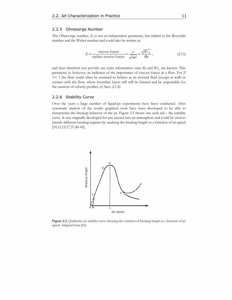
Over the years a large number of liquid-jet experiments have been conducted. After systematic analysis of the results graphical tools have been developed to be able to characterize the breakup behavior of the jet. Figure 2.3 shows one such aid – the stability curve. It was originally developed for jets ejected into an atmosphere and could be used to classify different breakup regimes by studying the breakup length as a function of jet speed [10,11,15,17,37,40-43].
A B
C
D
E
F
vcJet speed
Bre
akup len
gth
Figure 2.3. Qualitative jet stability curve showing the variation of breakup length as a function of jet speed. Adapted from [41].

12 Chapter 2. Liquid Jets
The initial part (ABC) of the stability curve, where the jet speed is not sufficiently high to create a jet, but only a train of drops, is referred to as the drip-flow regime. Once a jet is formed (point C), the breakup length increases proportionally with the jet speed up to about point D. In that region (CD) the effect of the ambient atmosphere is negligible and the breakup process of jets in this part of the curve is fairly well described by the analyses made by Rayleigh [6] and Weber [7], and is dominated by surface tension forces. In the literature it commonly referred to as Rayleigh breakup.
The longest possible coherent jet (point E) is generated at the so-called critical jet speed, vc, after which any further speed increase results in shorter breakup lengths (until point F is reached). This part (DEF) is called the wind-induced breakup regime and the shape of the breakup curve slightly past point E is well described by the stability theories developed by Sterling and Sleicher [10]. Beyond point F (spray regime) the disturbances due to atmospheric interactions are very large, and many different results of the coherent length of the jet have been reported. So far, there is no unifying theory that accurately predicts the breakup length of jets in this regime.
To further complicate the discussion, the onset of turbulence in the nozzle and velocity profile relaxation of the jet will also start influencing the breakup length at some stage in the stability curve. This does, however, depend very much on the specific experimental setup, and no general rules have been made to cover for that.
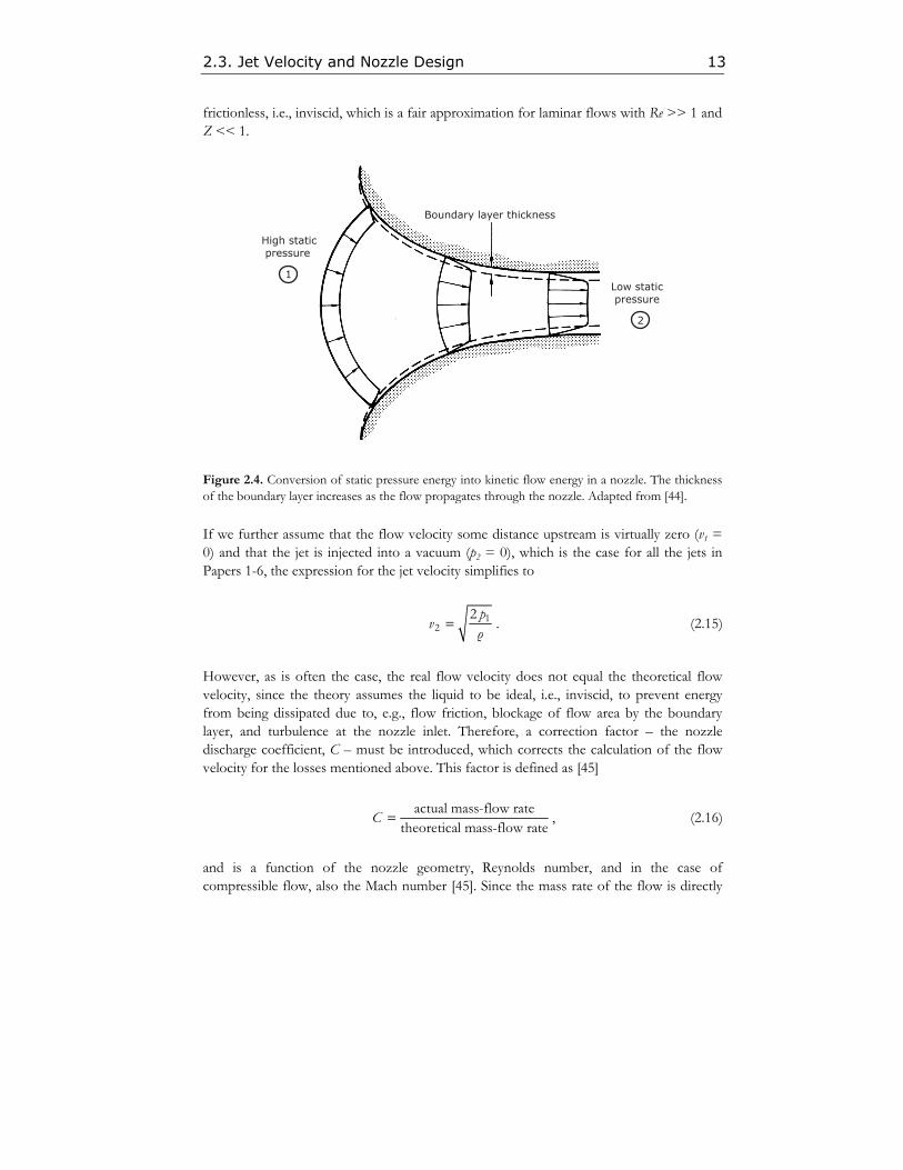
2.3 Jet Velocity and Nozzle Design A nozzle is a converging duct. The primary purpose of a nozzle is to convert static pressure energy into kinetic flow energy, and with proper design the efficiency of this energy conversion could be as high as 99% [44]. As the flow propagates through the convergent nozzle it is continuously accelerated, and boundary layers are formed along the nozzle surfaces. If the Re of the flow at the nozzle exit is >104 the boundary layers will be very thin in comparison to the nozzle diameter, unless for very long nozzles where the boundary layer eventually will fill the entire cross section of the flow [44] (cf. Sect. 2.1.4, and Figs. 2.1 and 2.4).
Assuming incompressible flow (ρ = const.) in the nozzle and that the pressure energy is perfectly transformed into kinetic energy in the nozzle, the equation for the conservation of the total pressure could be written as [44]
+ = +2 21 2
1 22 2ρv ρvp p , (2.14)
where p is the static pressure in the liquid, and the subscripts 1 and 2 refer to the different positions in Fig. 2.4 below. These presumptions are valid if the flow could be considered
2.3. Jet Velocity and Nozzle Design 13
frictionless, i.e., inviscid, which is a fair approximation for laminar flows with Re >> 1 and Z << 1.
Boundary layer thickness
High static pressure
1Low static pressure
2
Figure 2.4. Conversion of static pressure energy into kinetic flow energy in a nozzle. The thickness of the boundary layer increases as the flow propagates through the nozzle. Adapted from [44].
If we further assume that the flow velocity some distance upstream is virtually zero (v1 = 0) and that the jet is injected into a vacuum (p2 = 0), which is the case for all the jets in Papers 1-6, the expression for the jet velocity simplifies to
= 12
2 pvρ
. (2.15)
However, as is often the case, the real flow velocity does not equal the theoretical flow velocity, since the theory assumes the liquid to be ideal, i.e., inviscid, to prevent energy from being dissipated due to, e.g., flow friction, blockage of flow area by the boundary layer, and turbulence at the nozzle inlet. Therefore, a correction factor – the nozzle discharge coefficient, C – must be introduced, which corrects the calculation of the flow velocity for the losses mentioned above. This factor is defined as [45]
= actual mass-flow ratetheoretical mass-flow rate
C , (2.16)
and is a function of the nozzle geometry, Reynolds number, and in the case of compressible flow, also the Mach number [45]. Since the mass rate of the flow is directly
14 Chapter 2. Liquid Jets
proportional to the flow velocity, the expression for the flow speed at the nozzle exit in Eq. 2.15 modifies to
= 12
2 pv Cρ
. (2.17)
Numerical values for different nozzle shapes could, e.g., be found in Refs. 46-49. When striving for a discharge coefficient as close to unity as possible, there are some general guidelines to be followed. For instance, the contraction angle of the nozzle inlet in combination with streamlining of the interior of the nozzle is of major importance in order to prevent build-up of a thick boundary layer, create a more uniform velocity profile, and suppress the initiation of turbulence in the flow [17].
2.4 Liquid Jets in Vacuum The introduction of vacuum to the problem of generating a well-collimated jet has both pros and cons. One of the advantages is, of course, the negligible amplification of any disturbances due to atmospheric interactions (discussed in Sect. 2.1.3). On the other hand, a possible drawback is the introduction of the possibility of spontaneous bursting of the jet due to cavitation, which therefore is a subject in need of some further attention.
2.4.1 Cavitation
When the static pressure on a liquid body (at constant temperature) is reduced below a critical value (typically the vapor pressure) – either by static or dynamic means – spontaneous vaporization could occur, which is also referred to as cavitation. This should not be confused with boiling, which is vaporization of a liquid due to an increase of temperature at about constant pressure. The vaporization is initiated by the formation of a vapor void in the liquid body, a process usually referred to as nucleation. The nucleation phenomenon could also be divided into two different groups depending on the type of core that is responsible for the nucleation and growth of bubbles. Homogeneous nucleation is when thermal motions within the liquid form cores as microscopic voids, which could grow to macroscopic bubbles. This nucleation process generally occurs in very pure liquids in clean environments. However, in most ordinary engineering systems substantial amounts of small particles and other impurities are suspended in the liquid, which make excellent cores for bubble growth. The initiation of vaporization of the liquid in this manner is termed heterogeneous nucleation [50,51].
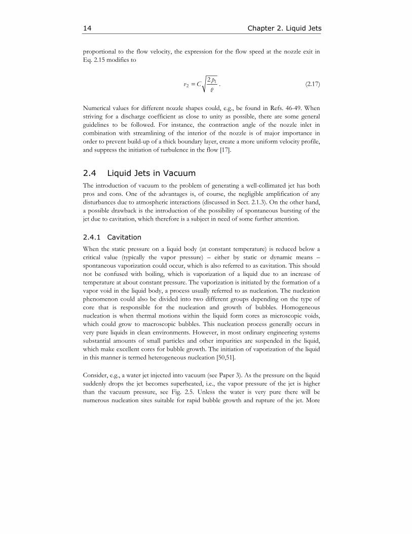
Consider, e.g., a water jet injected into vacuum (see Paper 3). As the pressure on the liquid suddenly drops the jet becomes superheated, i.e., the vapor pressure of the jet is higher than the vacuum pressure, see Fig. 2.5. Unless the water is very pure there will be numerous nucleation sites suitable for rapid bubble growth and rupture of the jet. More
2.4. Liquid Jets in Vacuum 15
information on the bubble growth dynamics and the potential bursting of a jet injected into vacuum can be found in Refs. 52-54.
T0p0 ,
Solid stateIce
Liquid state
Water
Gaseous state
Vapor
-50 0 50 100
10-1
1
10-2
10-3
10-4
Starting pointp0 ,T0
Superheatedwater jet
Endconditions
Evaporated gas flow
Inner part
Surface
Temperature (oC)
Am
bie
nt
pre
ssure
(at
m)
Figure 2.5. Phase diagram of a water jet injected into vacuum. Adapted from [53].
Cavitation could also occur inside the nozzle if the static pressure is substantially reduced, e.g., at a sharp bend. This is an unwanted effect, since the violent nature of a cavitation could result in considerable consequences for the performance of the nozzle due to, at least, two reasons: i) cavitations will effectively destroy any well-ordered flow, and ii) cavitation could damage the nozzle walls. Cavitation and its effects on adjacent solid boundaries are dealt with in more detail in Refs. 51, 55, and 56.
2.4.2 High-Speed Liquid-Metal Jets in Vacuum
This thesis is focused on the feasibility of making a high-brightness hard-x-ray source based on a liquid-metal-jet anode. One of the fundamental requirements for success is therefore a coherent, directionally stable, microscopic, high-speed liquid-metal jet in vacuum, which will be a regenerative electron-beam target, see Sect. 4.2. Without going into too much detail about the engineering-related problems this section will be devoted to a brief discussion on the metal jet.
As previously mentioned, injecting a jet into vacuum is connected with both advantages and disadvantages regarding the stability of the jet. The lack of atmosphere-related
16 Chapter 2. Liquid Jets
instabilities (cf. Sects. 2.1.3 and 2.2.6) should be weighed against the risk of cavitation in the jet. However, in the case of using metal as jet liquid the cavitation probability is practically zero, since the vapor pressure of most metals are well below any standard laboratory vacuum (~10-5 mbar in Papers 1-6). As an example, liquid tin at 300°C (m.p. 232°C) has a vapor pressure of ~10-19 mbar. Consequently, for a liquid-metal jet with such low vapor pressure the vacuum acts only beneficially from a coherence and stability point-of-view.
Directional stability has been shown not to be a major issue by experiments measuring the angular dispersion of a jet to about ±2 µrad for liquids with low vapor pressure [52,57,58]. There is no reason to believe that similar stabilities could not be achieved with liquid-metal jets provided that the liquid metal is satisfactorily pure and homogenous (cf. Paper 1). It is also important to have sufficient control over the heating process when preparing the liquid metal, since solidification close to the nozzle could seriously change the flow pattern, and, thus, also affect the jet performance.
The small diameter of the jet (<100 µm) also has pros and cons. Fluid mechanically it is an advantage, since (with everything else kept constant) it reduces the risk of turbulence (Re ∝ d), cf. Sect. 2.2.1. On the other hand, it could make the engineering somewhat troublesome. For instance, shaping of the nozzle to optimize jet performance may be mechanically difficult, and the sensitivity to solid particles in the liquid becomes rather high.
The requirement of a high-speed jet is probably one of the most difficult problems to solve. High speed requires a high driving pressure, and to make matters worse the high density of metals results in a need of even higher pressures compared to most other liquids. In order to create a ~500 m/s liquid-tin jet (further discussed in Sect. 4.2.2) about 10,000 bar of backing pressure must be obtained (cf. Eq. 2.15). A more exotic solution to this problem might be to combine a large electric current with a strong magnetic field applied over the metal reservoir. This might generate a driving force large enough to accelerate the molten metal to the required speed [59]. Whichever the final solution will be, it is quite likely to be an engineering challenge.

17
Chapter 3
Introductory X-Ray Physics
X-rays are electromagnetic radiation, just like, e.g., radio waves, microwaves, gamma rays, and visible light. The main difference between these types of radiation is the wavelength, or frequency, of the waves. A small part of the electromagnetic spectrum is shown in Fig. 3.1, and this thesis will only consider the part of the spectrum referred to as “hard x-rays”.
Photon energy (keV)
Wavelength (nm)
Figure 3.1. The electromagnetic spectrum from infrared (IR) to γ-rays.
Hard x-rays can be used to reveal internal structures and material properties of a wide range of optically opaque objects, such as a suitcase at an airport, a welding joint, or the heart of a living person. It is also possible to perform diffraction experiments to determine the structure of a crystal or to study the folding of proteins. The wide range of applications of hard x-ray sources in science, industry, and medicine is largely due to this penetrating property of the radiation. This chapter will briefly discuss production of x-rays and their interaction with matter from a semi-classical point-of-view [60,61]. More in-depth information on this topic, as well as the classical and quantum mechanical approach, could be found in a large number of standard textbooks, e.g., Refs. 62-65.
3.1 Electron-Matter Interaction When analyzing the electron-matter interaction, a distinction has to be made between thin and thick electron targets. A target is considered to be thin if the probability of more than one electron-matter interaction to occur during target passage is small. Conversely, an electron entering a thick target is likely to collide with many target atoms and deposit,
18 Chapter 3. Introductory X-Ray Physics
more or less, its entire kinetic energy to it. This discussion is restricted to thick targets only, since these theories apply to most standard x-ray tubes (cf. Section 4.1), as well as the liquid-metal-jet anode x-ray source (cf. Section 4.2 and Papers 1-6).
3.1.1 Atomic Configuration
An atom is made up of a nucleus consisting of protons and neutrons closely packed together at the center, and a cloud of orbiting electrons bound to the nucleus and arranged in different subshells. These shells are labeled K, L, M, and so forth counting from the center and out. The electrons in the innermost subshell are bound the strongest to the nucleus, and for each successive outward subshell the binding energies of the electrons are reduced. The K, and for the heavier elements even the L electrons, have binding energies in the x-ray range, which are only very weakly influenced by the surroundings of the atom. The much more loosely bound outer electrons are much more easily affected by the close environment and, thus, largely determine the chemical properties of the atom.
3.1.2 Electron Attenuation and Backscattering
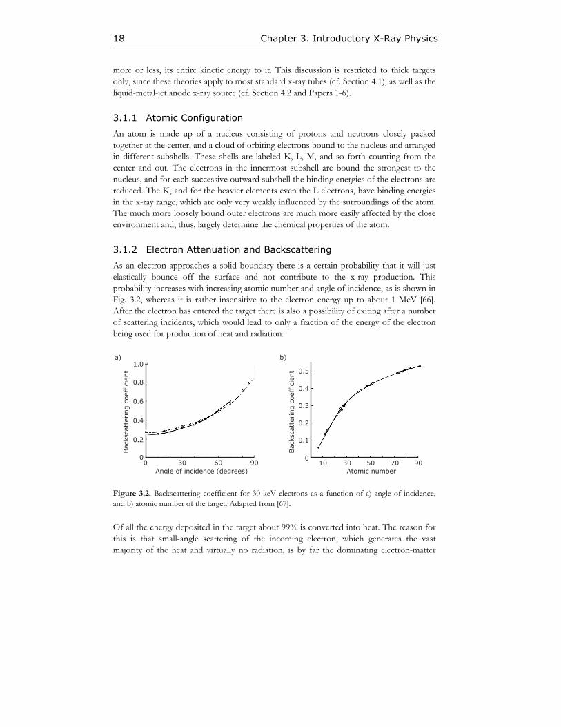
As an electron approaches a solid boundary there is a certain probability that it will just elastically bounce off the surface and not contribute to the x-ray production. This probability increases with increasing atomic number and angle of incidence, as is shown in Fig. 3.2, whereas it is rather insensitive to the electron energy up to about 1 MeV [66]. After the electron has entered the target there is also a possibility of exiting after a number of scattering incidents, which would lead to only a fraction of the energy of the electron being used for production of heat and radiation.
Angle of incidence (degrees)
0
0.2
0.4
0.6
0.8
1.0
Bac
ksca
tter
ing c
oef
fici
ent
300 60 90
a)
70503010 900
0.1
0.2
0.3
0.4
0.5
Atomic number
Bac
ksca
tter
ing c
oef
fici
ent
b)
Figure 3.2. Backscattering coefficient for 30 keV electrons as a function of a) angle of incidence, and b) atomic number of the target. Adapted from [67].
Of all the energy deposited in the target about 99% is converted into heat. The reason for this is that small-angle scattering of the incoming electron, which generates the vast majority of the heat and virtually no radiation, is by far the dominating electron-matter
3.1 Electron-Matter Interaction 19
interaction process. According to the classical theory, photons would be emitted every time the electron is deflected, but a quantum-mechanical treatment of the problem shows that the probability of that is very small for glancing deflections [68].
3.1.3 Continuous Bremsstrahlung
As mentioned above, only rarely will an incident electron be deflected through a large angle. This deflection is due to the Coulomb force between the electron and the heavily charged atomic nucleus. The larger the scattering angle, the more kinetic energy is lost during the event, which means more energy is emitted in the form of an x-ray photon, the so-called bremsstrahlung (or braking radiation). The intensity of the bremsstrahlung from a thick target has been found, both theoretically and experimentally, to obey the following expression [68]:
( ) ( )= −maxI hv CZ hv hv , (3.1)
where C is a constant, Z is the atomic number of the target atom, hνmax is the energy of the incident electron, and hν is the energy of the emitted bremsstrahlung photon. Figure 3.3a shows this dependence for a few different electron acceleration voltages. The total conversion efficiency, η, of the kinetic energy of the incident electron into emitted bremsstrahlung could be found by integrating Eq. 3.1, which results in
=η KZV , (3.2)
where K is a material constant, and V is the electron acceleration voltage in kilovolts. The theoretical value of K found by Kramers [60] is 9.2×10⁻⁷ kV-1. The experimentally found values are in good agreement with this, but with a slight dependence on Z. K ranges from 1.5×10⁻⁶ for aluminum (Z = 13) down to 7.5×10⁻⁷ for Z ~ 60 [69].
One particular property of the bremsstrahlung worth pointing out is the non-lambertian angular distribution, which makes it possible to increase the brightness of the radiation quite dramatically by observing the x-ray source at an angle (further discussed in Sect. 3.2.2). The angular and spectral distributions of the bremsstrahlung are shown in Fig. 3.3.

20 Chapter 3. Introductory X-Ray Physics
Anode 2080 60 40 20 806040 100%100%
0o10o10o
20o 20o
30o 30o
40o40o
50o 50o
60o 60o
70o 70o
80o 80o
90o 90o
8 16 504133250
8
7
6
5
4
3
2
1
Photon energy (keV)
Inte
nsi
ty (
a.u.)
19.8
29.4
39.3
49 keV
a) b)
1
2
3
Figure 3.3. a) Bremsstrahlung spectra for different electron energies. Adapted from [70]. b) Angular distribution of bremsstrahlung radiation from interaction of 70-keV electrons with a tungsten target. Curve 1 shows unfiltered radiation, curve 2 is radiation filtered with 10 mm of aluminum, and curve 3 describes the angular distribution according to the Lambert cosine law [71]. Adapted from [72].
3.1.4 Characteristic Line Emission and Auger Electrons
If an incident electron of sufficient energy knocks out an electron from, e.g., the K- or L-shell of the atom (given the Bohr atomic model), a vacancy is produced in the shell structure of the atom, as in Fig. 3.4a. That is a highly unstable state for an atom and the empty position is immediately (~10-11 s) filled by an electron from an outer shell. In this process, the energy difference between the two bound states is emitted in the form of a photon, see Fig. 3.4b. This photon is emitted in a random direction, and its energy, Eph, is characteristic to the element in question, and is calculated by using the following formula
( )∞⎛ ⎞
= − −⎜ ⎟⎜ ⎟⎝ ⎠
22 21 1
ph Kf i
E hcR Z σn n
, (3.3)
where h is Planck’s constant, c is the speed of light in vacuum, R∞ is the Rydberg constant, Z is the atomic number of the element, σK is a screening constant, n is the shell number, and the subscripts f and i stand for “final” and “initial”, respectively [73]. As the vacancy of the inner-shell electron is filled, a new hole is created in an outer shell, thus leading to another electron transition between an even more weakly bound electron and the new hole generating more characteristic radiation, but this time with a lower photon energy. This process repeats itself until all vacancies are filled, and the atom is stable again [74].
3.1 Electron-Matter Interaction 21
+ZeK
L
M
Primaryelectron
e-
e-
e-
Scatteredprimaryelectron
Secondaryelectron
KL
M
hv
+Ze
a) b)
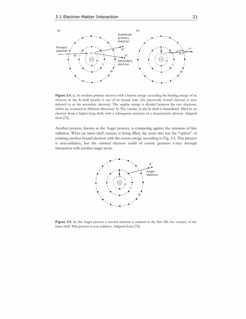
Figure 3.4. a) An incident primary electron with a kinetic energy exceeding the binding energy of an electron in the K-shell knocks it out of its bound state (the previously bound electron is now referred to as the secondary electron). The surplus energy is divided between the two electrons, which are scattered in different directions. b) The vacancy in the K-shell is immediately filled by an electron from a higher-lying shell, with a subsequent emission of a characteristic photon. Adapted from [75].
Another process, known as the Auger process, is competing against the emission of line radiation. When an inner-shell vacancy is being filled, the atom also has the “option” of emitting another bound electron with the excess energy according to Fig. 3.5. This process is non-radiative, but the emitted electron could of course generate x-rays through interaction with another target atom.
KL
M
Augerelectron
e-
+Ze
Figure 3.5. In the Auger process a second electron is emitted as the first fills the vacancy of the inner shell. This process is non-radiative. Adapted from [75].

22 Chapter 3. Introductory X-Ray Physics
Radiative decay as a hole in an inner shell is filled is proportional to Z4, whereas the likelihood of Auger emission of an electron is constant for all elements. This means that the probability of the emission of a characteristic photon, ω, is given by the ratio [76]
=+
4
4Zω
Z a, (3.4)
where a is a constant, e.g., for K-shell emission a = 1.12×10⁶. Thus, for elements with low Z the Auger process is dominating, while the situation is the reversed for heavy, high-Z electron targets.
3.2 X-Ray-Matter Interaction As x-rays penetrate matter some of the radiation is lost due to absorption and scattering. The dominating types of x-ray-matter interactions are the photoelectric absorption, coherent (Rayleigh) scattering, and incoherent (Compton) scattering. For higher photon energies (typically >1 MeV) other interaction possibilities also need to be considered, but they are outside the scope of this text.
Consider a large number, N0, of x-ray photons of a specific energy as they start to penetrate a piece of matter. According to Lambert’s law, “equal parts of the same absorbing medium attenuate equal fractions of the radiation” [77], which could be expressed mathematically in the form of the law of attenuation [78]:
−= 0attµ dN N e . (3.5)
Here, N is the number photons still unattenuated a distance d into the material, and µatt is the linear attenuation coefficient, which is a parameter depending on the x-ray energy, the element number and the density of the matter. The linear attenuation coefficient could be divided into two terms: the linear absorption coefficient, and the linear scattering coefficient. A very brief physical explanation of these parameters is found in the following two subsections.
3.2.1 Photoelectric Absorption
The photoelectric absorption (also called photoelectric effect or photo-ionization) is when an incoming x-ray photon interacts with a bound electron in an inner shell and transfers all of its energy to the electron, see Fig. 3.6. The energy of the photon must be larger than the binding energy of the electron, and the remaining energy is converted into kinetic energy for the emitted electron. The probability of photoelectric absorption increases with element number, but decreases with increasing photon energy [77,79].

3.2 X-Ray-Matter Interaction 23
Photoelectron
e-Photon
hv
E = hv - Eb
KL
M
+Ze
Figure 3.6. An incident photon can knock a bound electron out if the energy of the photon, hv, is larger than the binding energy of the electron, Eb. The surplus energy is transformed into kinetic energy, E, for the emitted photoelectron. Adapted from [75].
3.2.2 Scattering
The process of coherent (Rayleigh) scattering arise when the electric field of the incident x-ray photon interacts with a strongly bound electron, which is forced into vibration of the same frequency as the x-ray. These electrons will then emit dipole radiation with the same wavelength as the incoming radiation, i.e., without any loss of energy from the photon to the atom (Fig. 3.7a). The cross section for Rayleigh scattering is larger for lower x-ray energies and higher atomic numbers [80], see Fig. 3.8 below.
Eph
Eph
a) b)
Eph
Eph'
e-
'
Figure 3.7. a) In coherent, or Rayleigh, scattering the incident radiation interacts with a tightly bound electron and is scattered without any transfer of energy to the atom (Eph = E’ph). b) In the incoherent Compton scattering process the incident x-ray interacts with a loosely bound electron, which results in ionization. The scattered photon has lower energy than the incident photon (Eph > E’ph). Adapted from [81].

24 Chapter 3. Introductory X-Ray Physics
Incoherent (Compton) scattering, on the other hand, is a process where energy is transferred to the target atom. The scattering electron is only loosely bound to the atom and is upon collision with the x-ray photon knocked out of its orbit, leading to ionization of the atom, cf. Fig. 3.7b. Due to conservation of energy and momentum the scattered photon is then shifted towards a longer wavelength. The probability of Compton scattering is roughly the same for all x-ray energies and all materials [82], which could also be seen in Fig. 3.8.
10-2
100
102
104
106
Photon energy (keV)
10-2
100
102
104
106
Photon energy (keV)102101102101In
tera
ctio
n c
ross
sec
tion (
bar
n/a
tom
)
Carbon (Z=6) Lead (Z=82)
σtot
σtot
σRs
σRs
σCsσCs
σpa
σpa
Figure 3.8. The interaction cross section for some basic photon-matter interactions for carbon and lead in the energy range 5-300 keV. Subscript pa stands for photoelectric absorption, Rs for Rayleigh scattering, Cs for Compton scattering, and tot for the total cross section. Data generated by Ref. 83.
3.3 Index of Refraction X-rays are, just like visible light, electromagnetic waves. As an x-ray interacts with matter a phase change occurs due to coherent scattering. The amount of phase shift is determined by the refractive index, n, of the matter, which could be written as [84,85]
= − +1n δ iβ , (3.6)
where δ is the decrement of the real part of the refractive index responsible for the phase shift, and β is the imaginary term determining the absorption in the object. δ depends on both the radiation wavelength, λ, and the density, ρ, atomic number, Z, and atomic weight, A, of the object. For x-ray energies substantially larger than the K-absorption edge, δ could be written as [86]
=2 2
2 208π
A
e
N Zρe λδAε m c
, (3.7)
3.3 Index of Refraction 25
where e is the elementary charge, NA is Avogadro’s number, ε0 is the permittivity in vacuum, and me is the electron rest mass. This formula could be written in a more compact form by realizing that e2/4πε0mec2 is the expression for the classical electron radius, re, and that NAZρ/A is the electron density, ρe, in the object:
=2
2πe er λ ρδ . (3.8)
These simple expressions are only valid for radiation energies well above all absorption edges of the object. For most biological samples it should be satisfactorily accurate for x-rays above 10 keV, since the binding energies for K electrons in tissue and bone are typically in the range of a few hundred eV up to a few keV. The absorption term, β, may also be calculated if the linear absorption coefficient, µabs, is known [87]:
=4π
absλµβ . (3.9)
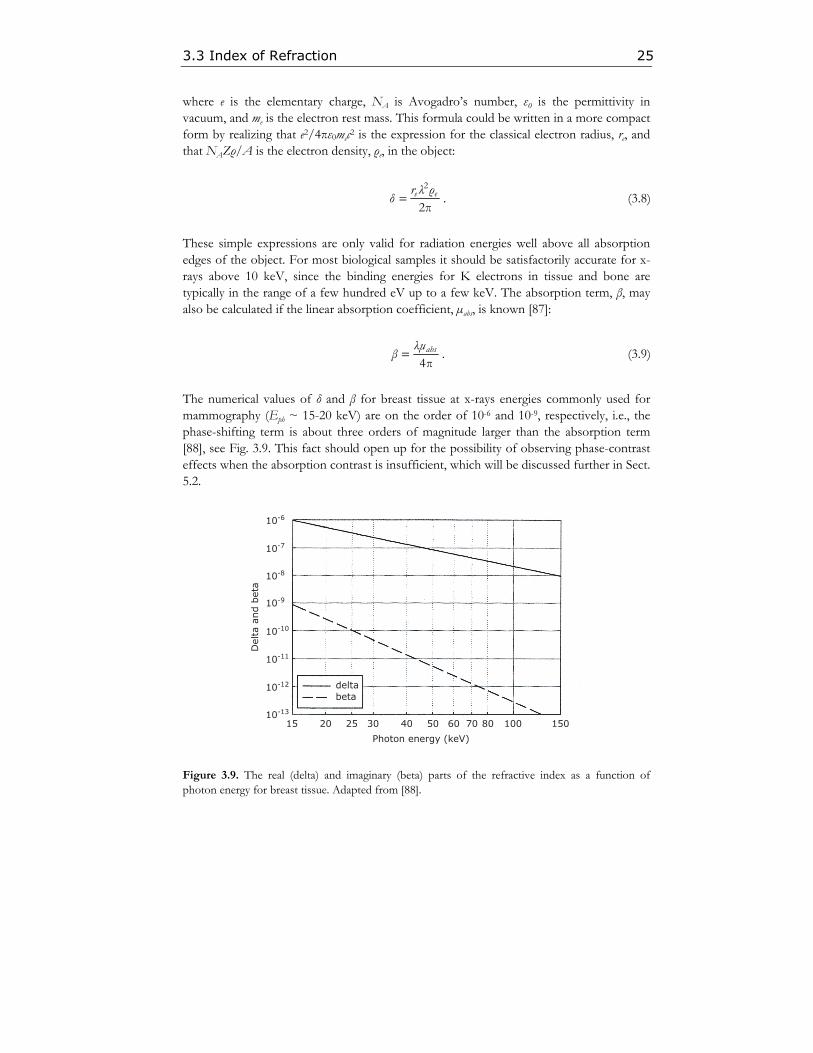
The numerical values of δ and β for breast tissue at x-rays energies commonly used for mammography (Eph ~ 15-20 keV) are on the order of 10-6 and 10-9, respectively, i.e., the phase-shifting term is about three orders of magnitude larger than the absorption term [88], see Fig. 3.9. This fact should open up for the possibility of observing phase-contrast effects when the absorption contrast is insufficient, which will be discussed further in Sect. 5.2.
10-6
10-10
10-8
10-7
10-9
10-11
10-12
10-13
deltabeta
Del
ta a
nd b
eta
2015 25 30 40 50 60 70 80 100 150
Photon energy (keV)
Figure 3.9. The real (delta) and imaginary (beta) parts of the refractive index as a function of photon energy for breast tissue. Adapted from [88].

27
Chapter 4
Electron-Impact X-Ray Sources
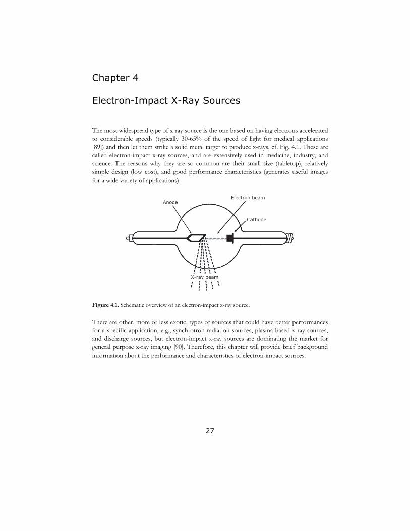
The most widespread type of x-ray source is the one based on having electrons accelerated to considerable speeds (typically 30-65% of the speed of light for medical applications [89]) and then let them strike a solid metal target to produce x-rays, cf. Fig. 4.1. These are called electron-impact x-ray sources, and are extensively used in medicine, industry, and science. The reasons why they are so common are their small size (tabletop), relatively simple design (low cost), and good performance characteristics (generates useful images for a wide variety of applications).
Anode
X-ray beam
Cathode
Electron beam
Figure 4.1. Schematic overview of an electron-impact x-ray source.
There are other, more or less exotic, types of sources that could have better performances for a specific application, e.g., synchrotron radiation sources, plasma-based x-ray sources, and discharge sources, but electron-impact x-ray sources are dominating the market for general purpose x-ray imaging [90]. Therefore, this chapter will provide brief background information about the performance and characteristics of electron-impact sources.

28 Chapter 4. Electron-Impact X-Ray Sources
4.1 Conventional Electron-Impact Sources As previously mentioned, most of the kinetic energy of the electrons is converted into heat as the electrons strike a target, and, thus, the anode plate needs to be appropriately cooled and made of a high-melting-point material. The choice of anode material is done after an analysis of the atomic number, maximum permissible temperature, specific heat, thermal conductivity, and the density of different elements. This analysis shows that tungsten is, in general, the best choice [91], but for some applications, e.g., mammography, a molybdenum anode is preferable due to its better match of characteristic line emission for that specific application.
Electron-impact x-ray sources can be divided into two main categories depending on the anode type: stationary-anode and rotating-anode tubes. Stationary-anode x-ray sources have, as the name implies, a non-moving anode, which makes the construction very reliable and robust. These are further discussed in Sect. 4.1.1. By letting the anode rotate it is possible to load a given target area with a larger electron-beam current and, thus, increase the x-ray flux by a factor of 5-10 [92]. The construction becomes more complex but for certain applications with high demands on the tube performance, such as computed tomography (CT), a rotating-anode x-ray source is preferred. More details about the rotating anode will be covered in Sect. 4.1.2.
4.1.1 Stationary-Anode Tubes
A typical stationary anode is a tungsten target embedded in a copper cooling block. The heat from the electron impact area is dissipated via conduction through the tungsten and copper to the surroundings. Additional heat removal could be attained by having a flow of water or oil passing close to the anode, but this is hardly ever used for diagnostics x-ray tubes.
Stationary-anode x-ray tubes have many applications in hospital environments, e.g., radiography and fluoroscopy. Such x-ray examinations are always a trade-off between maximizing image contrast and resolution (to be able to make a reliable diagnosis), and limiting the patient dose (to minimize the risk of causing radiation injuries). An additional requirement is to keep the exposure time as short as possible to reduce image blurring due to motion of the patient and, also, for comfort reasons.
X-ray sources for these applications have typical spot sizes between one and ten square millimeters, and operate at powers up to several kilowatts. The electron-beam impact spot on the anode is usually in the shape of a narrow rectangle. However, by observing the spot from an angle the x-rays will appear to originate from a square-shaped spot. This is called the line-focus principle and has two major benefits: the object “sees” a symmetrical x-ray source, which results in the same image resolution both vertically and horizontally, and the effective brightness of the source is substantially increased.

4.1 Conventional Electron-Impact Sources 29
The x-ray source brightness is a measure of the photon flux per unit solid angle and could be expressed in the unit photons/(s×mm2×mrad2). The spectral brightness is another frequently occurring source parameter, which is commonly measured in photons/(s×mm2×mrad2×0.1%BW). These units could be somewhat difficult to envision and the following text will therefore discuss the electron-beam power density on target instead (unit: kW/mm2). This switch could be done since the x-ray photon flux is proportional to the incident electron-beam power on the anode. For radiographic examinations the maximum power load on the anode surface is 0.1-1 kW/mm2, whereas fluoroscopy, which requires continuous source operation, has a limit of ~0.03 kW/mm2 [89].
Another type of stationary-anode tube is the microfocus source, which has a spot size of less than 100 µm and in some extreme cases even below 1 µm. These sources are run at much lower power (<50 W) and are typically used when studying non-living objects, e.g., examining the quality of solder joints or searching for cracks in machine parts. Even though these sources operate at such low effect, which yields quite long exposure times, they have a considerably higher power density limit at ~10 kW/mm2 and have found extensive use because of the very high image resolution that could be achieved due to their very small spot size (cf. Sect. 5.1).
4.1.2 Rotating-Anode Tubes
Already in 1896, the year after Roentgen’s discovery of x-rays, the American physicist R.W. Wood suggested that the e-beam power load capacity of an anode would increase if it could be rotated during the exposure [93]. However, the complexity of such an x-ray tube delayed the introduction of rotating-anode sources on the market until 1929 when Philips presented their Rotalix tube.
The main advantage of the rotating anode is an increase of the area that is targeted by the incoming electron beam, which leads to an enhanced heat dissipation. The e-beam power load limit, Plim, could be expressed as [89]
( )max
lim− −
=+
π ∆
1π
safety initiall T T T κρcfRdP
tfdkR
, (4.1)
where the parameters l, d, and R are defined in Fig. 4.2, κ is the thermal conductivity, ρ is the density, c is the specific heat capacity, f is the rotation frequency of the anode, t is the

30 Chapter 4. Electron-Impact X-Ray Sources
exposure time, and k is a correction factor depending on anode thickness, thermal radiation, and heat diffusion in the radial direction. The temperature Tmax is the upper limit in the focal spot before initiation of arc discharges between cathode and anode, which will disturb or interrupt the ongoing exposure. Therefore, a safety margin, ∆Tsafety, is used to avoid that kind of problem. Tinitial is the temperature of the anode before the start of the exposure.
Figure 4.2. Schematic view of a rotating anode and the utilization of the line-focus principle. Adapted from Paper 2.
The power density capacity on target of a modern rotating anode is ~10 kW/mm2 (~100 kW, ~1×10 mm2) for short electron-beam load times. As the exposure time is increased the maximum power load is reduced to avoid damaging the anode, see Fig. 4.3. Given a specific anode material composition the only way to increase this power load limit is to increase the rotation frequency and the radius of the disk [94]. But, since stable and fast rotation of large and heavy objects is difficult to obtain the performance of this type of source is practically limited by the engineering of the rotation mechanism.
4.1 Conventional Electron-Impact Sources 31
1000 mA
800 mA
700 mA
600 mA
500 mA
Maximum exposure time (s)
.01 .02 .04 .06 .1 .2 .4 .6 1 2 4 6 1030
150
140
130
120
110
100
90
80
70
60
50
40
Peak
voltag
e (k
V)
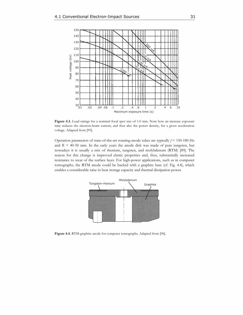
Figure 4.3. Load ratings for a nominal focal spot size of 1.0 mm. Note how an increase exposure time reduces the electron-beam current, and thus also the power density, for a given acceleration voltage. Adapted from [95].
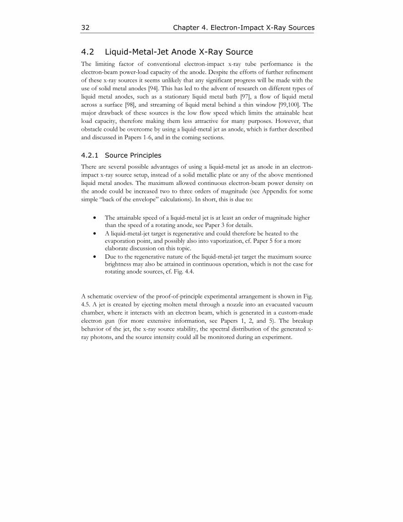
Operation parameters of state-of-the-art rotating-anode tubes are typically f = 150-180 Hz and R = 40-50 mm. In the early years the anode disk was made of pure tungsten, but nowadays it is usually a mix of rhenium, tungsten, and molybdenum (RTM) [89]. The reason for this change is improved elastic properties and, thus, substantially increased resistance to wear of the surface layer. For high-power applications, such as in computer tomographs, the RTM anode could be backed with a graphite base (cf. Fig. 4.4), which enables a considerable raise in heat storage capacity and thermal dissipation power.
Tungsten-rheniumMolybdenum
Graphite
Figure 4.4. RTM-graphite anode for computer tomographs. Adapted from [96].
32 Chapter 4. Electron-Impact X-Ray Sources
4.2 Liquid-Metal-Jet Anode X-Ray Source The limiting factor of conventional electron-impact x-ray tube performance is the electron-beam power-load capacity of the anode. Despite the efforts of further refinement of these x-ray sources it seems unlikely that any significant progress will be made with the use of solid metal anodes [94]. This has led to the advent of research on different types of liquid metal anodes, such as a stationary liquid metal bath [97], a flow of liquid metal across a surface [98], and streaming of liquid metal behind a thin window [99,100]. The major drawback of these sources is the low flow speed which limits the attainable heat load capacity, therefore making them less attractive for many purposes. However, that obstacle could be overcome by using a liquid-metal jet as anode, which is further described and discussed in Papers 1-6, and in the coming sections.
4.2.1 Source Principles
There are several possible advantages of using a liquid-metal jet as anode in an electron-impact x-ray source setup, instead of a solid metallic plate or any of the above mentioned liquid metal anodes. The maximum allowed continuous electron-beam power density on the anode could be increased two to three orders of magnitude (see Appendix for some simple “back of the envelope” calculations). In short, this is due to:
• The attainable speed of a liquid-metal jet is at least an order of magnitude higher than the speed of a rotating anode, see Paper 3 for details.
• A liquid-metal-jet target is regenerative and could therefore be heated to the evaporation point, and possibly also into vaporization, cf. Paper 5 for a more elaborate discussion on this topic.
• Due to the regenerative nature of the liquid-metal-jet target the maximum source brightness may also be attained in continuous operation, which is not the case for rotating anode sources, cf. Fig. 4.4.
A schematic overview of the proof-of-principle experimental arrangement is shown in Fig. 4.5. A jet is created by ejecting molten metal through a nozzle into an evacuated vacuum chamber, where it interacts with an electron beam, which is generated in a custom-made electron gun (for more extensive information, see Papers 1, 2, and 5). The breakup behavior of the jet, the x-ray source stability, the spectral distribution of the generated x-ray photons, and the source intensity could all be monitored during an experiment.

4.2 Liquid-Metal-Jet Anode X-Ray Source 33
CZT diode
Aperture
Pressure tank
Heater
Nozzle
Jet
CCD camera
E-beam dump
Pinhole cameraLaser illumination
E-beam gun
Figure 4.5. Proof-of-principle setup of the liquid-metal-jet anode electron-impact hard-x-ray source system and source diagnostics equipment. Adapted from Paper 2.
4.2.2 Performance Characteristics and Future Improvements
Typical performance characteristics of the present system:
• Metal jet: circular cross-section, down to ~20 µm diameter, 50-60 m/s max speed
• Electron gun: 600 W continuous operation (50 kV acceleration voltage, 12 mA electron-beam current), ~10 µm FWHM minimum focus spot size
A source spectrum from an experiment with a 30-µm diameter tin jet and a ~20 µm FWHM e-beam operated at 75 W is shown in Fig. 4.6. It has been corrected for detector efficiency, attenuation in filters, spot size, and measurement geometry to give the average spectral source brightness of the x-ray spot. The power density on the jet target is ~100 kW/mm2 within the FWHM, which is about 10× higher than state-of-the-art commercial electron-impact x-ray sources.

34 Chapter 4. Electron-Impact X-Ray Sources
20 504540353025Photon energy (keV)
0
6
5
4
3
2
1
×107
Spec
tral
brightn
ess
(ph/s
/mm
2/m
rad
2/0
.1%
BW
)
Figure 4.6. Source spectrum for a 75 W e-beam interacting with a 30-µm tin jet. The two peaks are the Kα and Kβ lines at 25.3 and 28.5 keV, respectively.
In principle, this could be increased at least one additional order of magnitude from today’s levels. For this to be realized the tin jet speed should be increased about a factor of ten to ~500 m/s (requires a driving pressure of 5,000-10,000 bar, see Paper 3). This improvement seems to be quite challenging from an engineering point-of-view, but there are no fundamental physical reasons that prevent it from being realized.

35
Chapter 5
X-Ray Imaging
Immediately after the discovery of x-rays in 1895 it found extensive use in society. The usefulness of being able to image the interior of a human body was instantly recognized and also practically utilized. Within a year, x-rays was a common diagnostic tool in medical practice both in Europe and in the US. X-ray imaging as a means of non-destructive testing of, e.g., machine parts and products in the industry was not introduced until about two decades later with the invention of the Coolidge tube [101]. This new type of x-ray source made it possible to generate acceleration voltages in excess of 100,000 volts, which is necessary to be able to penetrate thick metal objects.
As an introduction to this chapter about x-ray imaging, let us start by considering a plane electromagnetic wave in the x-ray region that is propagating parallel to the z-axis [102]:
( ) ( )0, i ωt kzz t e− −=E E , (5.1)
where E0 is the amplitude, ω is the angular frequency, and k is the wave number of the wave. At position z0 this wave strikes an object of thickness ∆z and complex refractive index n, which is given by (cf. Sect. 3.3)
1n δ iβ= − + . (5.2)
The wave number, k, of the radiation wave may be written on the form
( )1ωn ωk δ iβc c
= = − + , (5.3)
where c is the phase velocity of electromagnetic radiation in vacuum. The electromagnetic wave can upon exit from the object be represented by the expression
( ) ( )( )00
amplitude phase normal decay shiftpropagation
, i t k z z k z ik zz t e e e− − +∆ − ∆ − ∆=E E ω β δ , (5.4)

36 Chapter 5. X-Ray Imaging
where the first factor describes the wave if there had not been any object in its path, the second factor corresponds to the decay of wave amplitude due to radiation absorption in the object, and the third factor represents the modified phase shift due to the different refractive index of the object compared to the ambient medium.
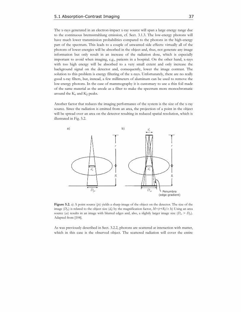
Different parts of the object absorb different amounts of x-rays, which results in substantially different values of the second term in Eq. 5.4 for different ray paths. This feature makes it possible to differentiate between, e.g., hard and soft tissue, and will be further discussed in Sect. 5.1. Another type of contrast mechanism utilizes the fact that the phase of the electromagnetic x-ray wave is changed when interacting with an object (the third term in Eq. 5.4). This could make it possible to detect and/or distinguish between almost non-absorbing objects. Different approaches of how to employ the phase shift in x-ray imaging are described in Sect. 5.2.
5.1 Absorption-Contrast Imaging If we place a detector behind the object considered above, an image of the integrated absorption along each x-ray path will be recorded, cf. Fig. 5.1. The detector records the intensity, I, which is proportional to the square of the time-averaged value of the electric field, E. This results in the following expression:
020
k zI I e−= β , (5.5)
where I0 is the intensity on the detector if the object was removed. This imaging technique yields clear and informative images when there are distinct absorption differences between different parts of the object. However, there are a few quality-degrading effects that need to be understood and, as far as possible, controlled in order to be able to acquire sharp absorption-contrast images.
X-Ray Tube
Object
Detector
Figure 5.1. Schematic view of the absorption-contrast imaging technique. Adapted from [103].
5.1 Absorption-Contrast Imaging 37
The x-rays generated in an electron-impact x-ray source will span a large energy range due to the continuous bremsstrahlung emission, cf. Sect. 3.1.3. The low-energy photons will have much lower transmission probabilities compared to the photons in the high-energy part of the spectrum. This leads to a couple of unwanted side effects: virtually all of the photons of lower energies will be absorbed in the object and, thus, not generate any image information but only result in an increase of the radiation dose, which is especially important to avoid when imaging, e.g., patients in a hospital. On the other hand, x-rays with too high energy will be absorbed to a very small extent and only increase the background signal on the detector and, consequently, lower the image contrast. The solution to this problem is energy filtering of the x-rays. Unfortunately, there are no really good x-ray filters, but, instead, a few millimeters of aluminum can be used to remove the low-energy photons. In the case of mammography it is customary to use a thin foil made of the same material as the anode as a filter to make the spectrum more monochromatic around the Kα and Kβ peaks.
Another factor that reduces the imaging performance of the system is the size of the x-ray source. Since the radiation is emitted from an area, the projection of a point in the object will be spread over an area on the detector resulting in reduced spatial resolution, which is illustrated in Fig. 5.2.
r
RR
r
do
Dps
do
Das
dsa) b)
Penumbra(edge gradient)
Figure 5.2. a) A point source (ps) yields a sharp image of the object on the detector. The size of the image (Dps) is related to the object size (do) by the magnification factor, M=(r+R)/r. b) Using an area source (as) results in an image with blurred edges and, also, a slightly larger image size (Das > Dps). Adapted from [104].
As was previously described in Sect. 3.2.2, photons are scattered at interaction with matter, which in this case is the observed object. The scattered radiation will cover the entire
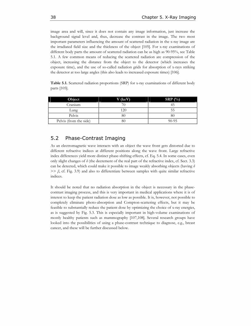
38 Chapter 5. X-Ray Imaging
image area and will, since it does not contain any image information, just increase the background signal level and, thus, decrease the contrast in the image. The two most important parameters influencing the amount of scattered radiation in the x-ray image are the irradiated field size and the thickness of the object [105]. For x-ray examinations of different body parts the amount of scattered radiation can be as high as 90-95%, see Table 5.1. A few common means of reducing the scattered radiation are compression of the object, increasing the distance from the object to the detector (which increases the exposure time), and the use of so-called radiation grids for absorption of x-rays striking the detector at too large angles (this also leads to increased exposure times) [106].
Table 5.1. Scattered radiation proportions (SRP) for x-ray examinations of different body parts [105].
Object V (keV) SRP (%) Cranium 70 45
Lung 120 55 Pelvis 80 80
Pelvis (from the side) 80 90-95
5.2 Phase-Contrast Imaging As an electromagnetic wave interacts with an object the wave front gets distorted due to different refractive indices at different positions along the wave front. Large refractive index differences yield more distinct phase-shifting effects, cf. Eq. 5.4. In some cases, even only slight changes of δ (the decrement of the real part of the refractive index, cf. Sect. 3.3) can be detected, which could make it possible to image weakly absorbing objects (having δ >> β, cf. Fig. 3.9) and also to differentiate between samples with quite similar refractive indices.
It should be noted that no radiation absorption in the object is necessary in the phase-contrast imaging process, and this is very important in medical applications where it is of interest to keep the patient radiation dose as low as possible. It is, however, not possible to completely eliminate photo-absorption and Compton-scattering effects, but it may be feasible to substantially reduce the patient dose by optimizing the choice of x-ray energies, as is suggested by Fig. 5.3. This is especially important in high-volume examinations of mostly healthy patients such as mammography [107,108]. Several research groups have looked into the possibilities of using a phase-contrast technique to diagnose, e.g., breast cancer, and these will be further discussed below.

5.2 Phase-Contrast Imaging 39
3.0
2.0
1.0
0.80.70.60.5
0.4
0.3
0.215 20 30 40 50 60 70 80 100 150
Photon energy (keV)
KERM
A (
µG
y/10
6 p
hoto
ns/
cm2)
Figure 5.3. The kinetic energy released in matter (KERMA) as a function of photon energy for breast tissue. Adapted from [88].
There are three different approaches to use the phase information to increase the image contrast: x-ray interferometry, diffraction-enhanced imaging, and in-line phase contrast. The physics of these methods will be briefly described in the following subsections, along with some of the benefits and drawbacks, and why this contrast mechanism is currently not used in, e.g., everyday diagnostics in hospitals.
5.2.1 X-Ray Interferometry
Information about optical properties and/or geometrical features of the object can be revealed by detecting the phase change of electromagnetic radiation in an interferometer [109]. This is just as true for x-rays as it is for optical wavelengths. The experimental arrangement of an x-ray interferometer is depicted in Fig. 5.4, which shows an x-ray beam from a synchrotron radiation source being monochromatized by Bragg diffraction [110] in a silicon crystal and divided into two separate coherent waves in the splitter crystal. These waves are reflected back towards each other in the mirror crystal after which a sample is placed in one of the beam paths. Finally, the waves overlap again at the analyzer crystal where they set up an interference pattern, which is recorded by the detector. This method has been used to detect density variation as small as 10-9 g/cm3 in biological samples [111], which is enough to be able to separate healthy tissue from cancer tumors in, e.g., breast, liver, and kidney.

40 Chapter 5. X-Ray Imaging
Synchrotron Radiation
MonochromatorSplitter Mirror Analyzer
Object
Detector
Figure 5.4. Experimental setup for x-ray interferometry. Adapted from [111].
The radiation source for this type of phase-contrast imaging is virtually always a synchrotron. The main reason for that is their very high spectral brightness which typically ranges from ~1015 to ~1019 photons/(mm2×s×mrad2×0.1%BW) [112,113]. This number should be compared to the ~109 photons/(mm2×s×mrad2×0.1%BW) of the Sn-Kα peak of the liquid-metal-jet anode source (cf. Paper 4), and it becomes quite clear that x-ray interferometry using a compact electron-impact x-ray source would result in extremely long exposure times and is, thus, practically useless.
5.2.2 Diffraction-Enhanced Imaging
The experimental arrangement for diffraction-enhanced imaging (DEI) is simpler than the one for x-ray interferometry, as can be seen in Fig. 5.5a. DEI is most often used with monochromatic radiation, which is accomplished in a similar manner as in the interferometry case utilizing Bragg diffraction in a crystal. The radiation that strikes the object is essentially parallel and can interact with it in a few different ways: it may be absorbed, scattered (coherently or incoherently) into a large span of angles (see Fig. 5.6), or refracted with angles of the order of microradians [111]. The refraction angles are proportional to the gradient of the real part of the refractive index, and due to the very small deviations from unity of δ (cf. Sect. 3.3) the refraction angles are also very small.
X-RaysMonochromator
Object
Analyzer
Detector
Ref
lect
ivity
-5 50Angle (µrad)
a) b)
Figure 5.5. a) Experimental arrangement for diffraction-enhanced imaging. b) An example of a rocking curve for the analyzer crystal. Adapted from [111].

5.2 Phase-Contrast Imaging 41
Behind the object is a so-called analyzer crystal, whose reflectivity depends on the incident angles of the x-rays. The reflectivity strongly depends on the angle of incidence (falls down to zero for angles of ±5-10 µrad off the peak reflection angle) and is called the rocking curve of the crystal, cf. Fig. 5.5b. If the analyzer is aligned for maximum reflection of the non-scattered transmitted radiation, the image on the detector will look like a standard radiograph, but with better contrast due to the rejection of the scattered x-rays. By slightly adjusting the tilting angle of the crystal to where the refracted photons are reflected the most leads to dramatically increased contrast of refractive index gradients.
Figure 5.6. Probability functions for a) Rayleigh scattering and b) Compton scattering for three different photon energies interacting with a water target. Each curve is normalized to 100% for the most likely scattering angle. Adapted from [114].
By using this technique, the x-ray image will clearly show the boundaries between parts of the object with different refractive indices [111], cf. Fig. 5.7 below. DEI could also be used to separate absorption and phase-contrast effects by combining two images taken on either side of the rocking curve [111,115].
a) b)
Figure 5.7. a) Digital radiograph (standard absorption-contrast image) and b) diffraction-enhanced image of the same breast tissue sample [116]. The arrows indicate areas of interest for mammography specialists.

42 Chapter 5. X-Ray Imaging
A number of studies have examined the visibility of features in x-ray images using DEI as a function of absorbed dose in the tissue. These investigations have mainly studied breast tissue in the search for tumors [108,116-118], but also cartilage [119], tendons and ligaments [120], and lungs [121]. Although most of these studies have been done at synchrotron facilities this is not necessary. Ingal et al. [108] have performed DEI experiments using an electron-impact source with an Ag anode (Kα line @ 22.2 keV) operated at an e-beam power density of ~15 kW/mm2. The required exposure time to record a high-quality DEI mammogram was about 20 min, but they argue that this could be reduced to 1-10 s with a better choice of commercially available x-ray sources and detectors. This statement makes it plausible that the exposure times using the metal-jet-anode concept in Papers 1-6 could be reduced another order of magnitude due to the much higher power density capacity and, thus, be clinically acceptable. The potential improvement in making more accurate diagnoses and reducing patient dose by introducing DEI as a tool in the search of, e.g., breast cancer, certainly warrants further experimental studies in this field.
5.2.3 In-Line Phase-Contrast Imaging
The simplest way to image the phase information of an object is the in-line phase-contrast method. This imaging technique has many different names in the literature, e.g., in-line holography, out-line phase contrast, and phase-propagation imaging. Whereas the experimental arrangements in Sects. 5.2.1 and 5.2.2 require rather elaborate optics the only requirements here are a source with moderate spatial coherence, a sufficient flux to keep exposure times reasonable, and some distance between the object and the detector, cf. Fig. 5.8.
d
X-Rays
Object
Detector
Figure 5.8. Experimental arrangement for in-line phase-contrast imaging. Adapted from [111].
The theory of in-line phase-contrast imaging could be described fairly well in a few simple steps. More in-depth information on this subject could be found in, e.g., Refs. 121-126. The total x-ray phase change relative to vacuum, φ, as a function of the transverse coordinates (x, y) in the object is found in the third term in Eq. 5.4:
( ) ( ), ∆ ,φ x y k zδ x y= , (5.6)

5.2 Phase-Contrast Imaging 43
if the thickness of the object is ∆z. The absorption in the object can in a similar manner be expressed as (cf. Eq. 5.5)
( ) ( ), 2 ∆ ,µ x y k zβ x y= . (5.7)
Given Eqs. 5.6 and 5.7, an incident plane wave e-i(ωt-kz) may immediately after interaction with the object (located at position z0) be described by the following wave function
( ) ( )( ) ( ) ( )0 ∆ , , /2, i ωt k z z iφ x y µ x yf x y e e− − + −= ⋅ . (5.8)
By placing a detector immediately behind the object it should be noted that no phase information will be recorded in the image, since the image intensity, I, is given by
( ) ( )−= =2 ,, µ x yI f x y e . (5.9)
An interesting special case of in-line phase-contrast imaging is when the object is thin and/or only weakly interacting with the radiation, as is the case for the image of the latex spheres in Paper 4. The transmission function, q(x,y) , which is the second factor in Eq. 5.8, can after Taylor expansion be written as
( ) ( ) ( ) ( ) ( )−= + −, , /2, 1 , , / 2iφ x y µ x yq x y e iφ x y µ x y , (5.10)
which could be even further simplified by neglecting the absorption:
( ) ( )+, 1 ,q x y iφ x y . (5.11)
Under the assumption of negligible absorption, an expression for the intensity in a plane behind the object can be represented in Fourier space [124,125]:
( ) ( ) ( )+, , 2Φ , sinzI u v δ u v u v χ , (5.12)
where it is important not to confuse the Dirac delta function, δ(u,v), with the decrement of the real part of the refractive index, δ, cf. Eqs. 3.6-3.8. Ф is the Fourier transform of φ, the variables u and v denote the transverse spatial frequencies in Fourier space, and χ = πλz(u2+v2). By working in the so-called near-field region where χ is much smaller than π/2 Eq. 5.12 may be slightly modified by using sin χ ≈ χ resulting in:
( ) ( ) ( ) ( )2 2, , 2π Φ ,zI u v δ u v λz u v u v+ + . (5.13)

44 Chapter 5. X-Ray Imaging
Taking the inverse Fourier transform of Eq. 5.13 yields an expression for the pure phase-contrast intensity a distance z behind the object:
( ) ( )⊥= − ∇2, 1 ,2πzλzI x y φ x y , (5.14)
where 2⊥∇ is the two-dimensional Laplacian acting on φ(x, y). Combining this formula
with Eqs. 3.8 and 5.6 results in the following expression:
( ) ( )( )2, 1 ,ez e
λzrI x y ρ x y dzk ⊥= − ∇ ∫ , (5.15)
where re is the classical electron radius, and ρe is the electron density in the object. This Laplacian will turn up on the detector as an edge-enhancement in the form of a sharp black and white fringe, as in Fig. 5.9 below. It should also be noted that the location of this fringe is independent of the wavelength of the radiation. Hence, unlike the phase-contrast mechanisms described in the two previous sections, there is not a very strict limitation to the spectral bandwidth of the x-ray source for in-line phase-contrast imaging.
Figure 5.9. In-line phase-contrast image of objects with insignificant absorption. On the left there is a cable tie of nylon with a thickness of 0.75 mm. Note the dark and bright fringes at sharp edges. On the right side there is a feather with some 100-µm diameter polystyrene spheres attached to it.
Spatial coherence, on the other hand, is of much more importance. In short, each point in the x-ray emitting area generates a diffraction pattern of the object at slightly different locations on the detector. The overall intensity distribution is found by adding the individual images, which results in more blurring with increasing source size. A more elaborate discussion on spatial coherence considerations and implications could be found in several articles, e.g., Refs. 124-126.
The main reason this imaging technique has not yet found any place in clinical examinations is the very long exposure times needed (several minutes) with conventional

5.2 Phase-Contrast Imaging 45
electron-impact sources. To meet the requirement of spatial coherence the source size must be quite small, which by necessity results in rather lengthy exposures [123-125] due to the low power-load capacity of conventional sources, and the long propagation distance between object and detector that is needed. The future may prove that further development of the liquid-metal-jet anode source may be a way to make it practically feasible to implement phase-contrast imaging into standard x-ray diagnostics.


47
Appendix
This appendix will, by using a very simple physical model of the interaction between the electron beam and the liquid-tin jet, show that the attainable electron-beam power density is 100-1000 times higher than for rotating anode x-ray sources.
By assuming a cylindrical liquid-tin jet with diameter d, which is struck by an electron beam of the same diameter d, the required power to fully evaporate the targeted volume segment may be calculated. In combination with the interaction area between the tin jet and the electron beam, the electron-beam power density is given. This is only an approximate calculation to indicate the potential of the heat load capacity of this type of anode. Considerable refinement of this model is needed to generate a more accurate result.
Liquid-tin jet parameters:
• Speed, v: 500 m/s • Jet temperature, Tjet: 300°C • Density @ Tjet, ρ: 7.0×10³ kg/m3 • Boiling temperature @ pvacuum ~10-4 mbar, Tboil: ~1000°C • Specific heat capacity, cp: 230 J/(kg K) • Heat of vaporization, Evap: 2.45×10⁶ J/kg
By combining Eqs. 3 and 4 in Paper 2, the following expression for the electron-beam power density required for complete evaporation of the intersection volume of the tin jet and the electron beam may be calculated (cf. Fig. 2 in Paper 2):
( )p boil jet vapP ρv c T T EA
⎡ ⎤= − +⎣ ⎦ , (A.1)
which results in 9 MW/mm2, which is about three orders of magnitude more than for rotating-anode sources (cf. Sect. 4.1.2).

49
Summary of Papers
This thesis is based on the six papers listed below. They are all directed towards the development of a compact high-brightness hard-x-ray source based on a liquid-metal-jet anode. The author has been main responsible for Papers 3, 5, and 6. In the other papers the author has been actively involved in the planning, preparation, and performing of the experiments, however not in the design of the electron gun or the details of the imaging calculations.
Paper 1
This paper introduces a new liquid-metal-jet anode concept for electron-impact sources. Initial calculations show that this could potentially increase the attainable brightness in compact x-ray tubes by more than a factor 100. The x-ray source is demonstrated in a low-power, proof-of-principle experiment verifying the basic concept.
Paper 2
In this paper there is a more extensive demonstration of the liquid-metal-jet anode concept and the low-power system. An anode-material figure-of-merit depending on thermal properties and x-ray conversion efficiency is developed, and the system details are described. High-power scaling and source limitations are also discussed.
Paper 3
This paper investigates the fluid mechanics of microscopic high-speed liquid-metal-jets in vacuum by dynamic-similarity experiments using water. It is shown that the vacuum environment prevents wind-induced breakups, but instead the possibility of jet breakup due to cavitation must be considered. It is concluded that a 30-µm diameter, 500-m/s liquid-tin jet in vacuum should be possible to generate, and that cavitation is not of any concern for metal jets.
Paper 4
In this paper the high-brightness liquid-tin-jet x-ray source is used for high-resolution phase-contrast imaging of weakly absorbing objects, and it is showed that this contrast mechanism also could increase the observable resolution. The jet-anode concept is operated at an electron-beam power density about an order of magnitude higher than state-of-the-art solid metal anodes.

50 Summary of Papers
Paper 5
This paper investigates the feasibility of scaling the power and power density to levels close to the fundamental limit set by the cathode. Potential obstacles to this improvement such as instabilities of the x-ray spot and the debris emission are discussed. The impact of varying the speed and size of the metal-jet target is also briefly examined.
Paper 6
In this paper a 9-keV source based on a liquid-gallium jet is demonstrated. An improved e-beam focusing lens makes it possible to attain ~10-µm spots at high power-density levels. A brightness spectrum is recorded and future source improvements along with possible applications such as crystallography and microscopy are discussed.

51
Acknowledgements
I have been fortunate to spend the last few years at the department of Biomedical & X-Ray Physics together with a very interesting group of people of vast diversity. This has led to an inevitable development, not only of the x-ray source concept described in this thesis, but also of me, if I may say so myself. Therefore, there are a number of people that I feel a great need to acknowledge.
First of all, I would like to thank my professor, Hans Hertz. His very straightforward and pragmatic approach to how to think about physics has made a major impact on me. Combining this with his leadership of this department by the example of always being open to new ideas, work hard, and a sincere interest in his students’ well-being, he is as close as you get to the ultimate supervisor.
A big thank you goes to Tomi Tuohimaa, a great co-worker and an even better friend. Thanks to his never-ending supply of new ideas he has been a major reason to why this work has been so much fun.
Special thanks also to Oscar Hemberg, who taught me a lot about how to think about and deal with applied physics in general and metal-jet x-ray machines in particular.
I would also like to thank:
Jalmar Thoresen for his splendid assistance during the many, and sometimes tedious, water-jet experiments.
Magnus Lindblom, Anders Holmberg, Martin Wiklund, and Ulrich Vogt for the many lunches together that almost always result in some interesting discussion.
The rest of my past and present colleagues at the department: Michael Bertilsson, Klaus Biedermann, Kjell Carlsson, Mats Gustafsson, Jaco de Groot, Anna Gustrin, Björn Hansson, Jessica Hultström, Göran Johansson, Elle Kristiansson, Anders Liljeborg, Linda Lundström, Göran Manneberg, Otto Manneberg, Karolina Pihlblad, Milan Pokorny, Stefan Rehbein, Heide Stollberg, Per Takman, Peter Unsbo, and Nils Åslund.
Rolf Helg and Kjell Hammarström for great service in the mechanical workshop, and without whom none of my work could have been done.

52 Acknowledgements
Gustav Amberg for the interesting and valuable discussions on various fluid mechanics problems.
Seshadri Seetharaman for all the help regarding properties of molten metals.
Also, Cecilia Heyman in the Albanova library deserves many thanks for her fast and excellent service.
Finally I would like to express the gratitude I feel to my family. They are, by far, the most important people in my life. Despite the many difficulties in the past few years, my family has always been there to support, inspire and encourage me to strive for something more, and for that I owe you. Much to my regret, my father, Leif, cannot share this moment with me. I would have liked that.

53
Bibliography
[1] W. C. Röntgen, ”Über eine neue Art von Strahlen”, Sitzungsberichte Med. Phys. Gesellshaft Würzburg, pp. 137-141 (1895).
[2] M. V. Klein, Optics (John Wiley & Sons, New York, 1970), Chapter 4.1 – Radiometry and Photometry, pp. 132-134.
[3] G. Bidone, ”Expériences sur la Forme et sur la Direction des Veines et des Courants d´Eau Lances par Diverses Ouvertures”, Imperiale Royale, Turin, pp. 1-136 (1829).
[4] F. Savart, ”Memoire sur la Constitution des Veines Lequides Lancees par des Orifices Circulaires en Mince Paroi”, Ann. Chim. Phys. 53, 337-386 (1833).
[5] J. Plateau, Statique Expérimentale et Théorique des Liquides Soumis aux Seules Forces Moléculaires (Canthier Vallars, Paris, 1873).
[6] L. Rayleigh, ”On the Instability of Jets”, Proc. London Math Soc. 10, 4-13 (1879).
[7] C. Weber, ”Zum Zerfall eines Flüssigkeitsstrahles”, Z. Angew. Math. Mech. 11, 136-159 (1931).
[8] D. J. Acheson, Elementary Fluid Dynamics (Oxford University Press, 1990), Chapter 2.1 – Elementary Viscous Flow – Introduction, pp. 26-30.
[9] R. F. Probstein, Physicschemical Hydrodynamics (John Wiley & Sons, New York, 1994), 2nd ed., Chapter 2.2 – Viscosity and Momentum Transport, pp. 10-17.
[10] A. M. Sterling, and C. A. Sleicher, “The Instability of Capillary Jets”, J. Fluid Mech. 68, 477-495 (1975).
[11] R. P. Grant, and S. Middleman, ”Newtonian Jet Stability”, A.I.Ch.E. J. 12, 669-678 (1966).
[12] R. W. Fenn, and S. Middleman, ”Newtonian Jet Stability: The Role of Air Resistance”, A.I.Ch.E. J. 15, 379-383 (1969).
[13] B. J. Meister, and G. F. Scheele, “Prediction of Jet Length in Immiscible Liquid Systems”, A.I.Ch.E. J. 15, 689-699 (1969).
[14] D. J. Acheson, Elementary Fluid Dynamics (Oxford University Press, 1990), Fig. 8.6, p. 266.
54 Bibliography
[15] A. H. Lefebvre, Atomization and Sprays (Taylor & Francis, 1989), Chapter 2 – Basic Processes in Atomization, pp. 27-78.
[16] R. D. Blevins, Chapter 6.2 – Velocity Profiles for Fully Developed Pipe Flow, pp. 39-42, in [23].
[17] M. J. McCarthy, and N. A. Molloy, “Review of Stability of Liquid Jets and the Influence of Nozzle Design”, Chem. Eng. J. 7, 1-20 (1974).
[18] A. H. Lefebvre, Atomization and Sprays (Taylor & Francis, 1989), Fig. 2.9, p. 46.
[19] R. D. Reitz, Atomization and Other Breakup Regimes of a Liquid Jet, Ph.D. Thesis, Princeton University, 1978, Chapter 2.5.4 – Velocity Profile Rearrangement and Jet Breakup, pp. 37-39.
[20] R. E. Phinney, ”The Breakup of a Turbulent Liquid Jet in a Gaseous Atmosphere”, J. Fluid Mech. 60, 689-701 (1973).
[21] P. H. Schweitzer, ”Mechanisms of Disintegration”, Penn. State Coll. Eng. Exp. Sta. Bull. No. 40, Appendix I, pp. 63-66 (1932).
[22] J. F. Douglas, J. M. Gasiorek, and J. A. Swaffield, Fluid Mechanics (Longman Scientific & Technical, Essex, 1995), 3rd ed.
[23] R. D. Blevins, Applied Fluid Dynamics Handbook (Krieger Publishing Company, Florida, 1992), reprint ed.
[24] W. M. Rohsenow, J. P. Hartnett, and E. N. Ganić, eds., Handbook of Heat Tranfer Fundamentals (McGraw-Hill, New York, 1985), 2nd ed.
[25] F. P. Incropera, and D. P. DeWitt, Fundamentals of Heat and Mass Transfer (Wiley, New York, 1996), 4th ed.
[26] J. F. Douglas, J. M. Gasiorek, and J. A. Swaffield, Chapter 8 – Dimensional Analysis, pp. 233-255, in [22].
[27] W. M. Rohsenow, J. P. Hartnett, and E. N. Ganić, Chapter 8B-2 – Dimensional Groups of Flow and Transport Parameters, p. 8-8, in [24].
[28] R. D. Blevins, Chapter 4 – Dimensional Analysis, pp. 8-17, in [23].
[29] E. Buckingham, ”Model Experiments and the Forms of Empirical Equations”, Trans. A.S.M.E. 37, 263-296 (1915).
[30] J. F. Douglas, J. M. Gasiorek, and J. A. Swaffield, Chapter 8.13 – Dimensional Analysis by the Group Method, pp. 247-251, in [22].

55
[31] J. F. Douglas, J. M. Gasiorek, and J. A. Swaffield, Chapter 9.2 – Dynamical Similarity, pp. 262-267, in [22].
[32] D. J. Tritton, Physical Fluid Dynamics (Clarendon Press, Oxford, 1988), 2nd ed., Chapter 7 – Dynamical Similarity, pp. 89-96.
[33] F. P. Incropera, and D. P. DeWitt, Chapter 8.1.1 – Flow Conditions, pp. 420-421, in [25].
[34] R.E. Phinney, ”Stability of a Laminar Viscous Jet – The Influence of the Initial Disturbance Level”, A.I.Ch.E. J. 18, 432-434 (1972).
[35] R. D. Reitz, Atomization and Other Breakup Regimes of a Liquid Jet, Ph.D. Thesis, Princeton University, 1978, Chapter 1.3 – Four Regimes of Jet Breakup, pp. 4-9.
[36] R. E. Phinney, ”Stability of a Laminar Viscous Jet – The Influence of an Ambient Gas”, Phys. Fluids 16, 193-196 (1973).
[37] S. P. Lin, and R. D. Reitz, ”Drop and Spray Formation from a Liquid Jet”, Annu. Rev. Fluid Mech. 30, 85-105 (1998).
[38] R. D. Blevins, Chapter 4.5 – Mach Number, p. 11, in [23].
[39] J. F. Douglas, J. M. Gasiorek, and J. A. Swaffield, Chapter 9.4 – Zone of Dependence of Mach Number, pp. 269-270, in [22].
[40] S. Leroux, C. Dumouchel, and M. Ledoux, “The Break-up Length of Laminar Cylindrical Jets. Modification of Weber’s Theory”, Int. J. Fluid Mech. Res. 24, 428-438 (1997).
[41] R. D. Reitz, and F. V. Bracco, “Mechanisms of Breakup of Round Liquid Jets”, Chapter 10 in The Encyclopedia of Fluid Mechanics (Gulf, Houston, 1986).
[42] R. D. Reitz, Atomization and Other Breakup Regimes of a Liquid Jet, Ph.D. Thesis, Princeton University, 1978, Fig. 1.1, p. 165.
[43] R. D. Blevins, Chapter 9.6.1 – Liquid Jets in Gases, pp. 262-264, in [23].
[44] R. D. Blevins, Chapter 7.2 – Theoretical Nozzle Performance, pp. 124-136, in [23].
[45] R. D. Blevins, Chapter 7.3 – Nozzle Discharge Coefficient, pp. 136-143, in [23].
[46] R. D. Blevins, Table 7.5 – Nozzle Discharge Coefficients, pp. 139-141, in [23].
[47] V. I. Asihmin, Z. I. Geller, and Y. A. Skobelcyn, ”Discharge of a Real Fluid from Cylindrical Nozzles”, Oil Ind. 9, 135-172 (1961).
[48] R. P. Benedict, and J. S. Wyler, “Analytical and Experimental Studies of ASME Flow Nozzles”, Trans. ASME J. Fluids Eng. 100, 265-275 (1978).

56 Bibliography
[49] Y. Nakayama, ”Action of Fluid in the Air Micrometer: First Report, Characteristics of Small Diameter Nozzle and Orifice”, Bull. Jap. Soc. Mech. Eng. 4, 516-541 (1961).
[50] C. E. Brennen, Cavitation and Bubble Dynamics (Oxford University Press, 1995), online ed., Chapter 1 – Phase Change, Nucleation, and Cavitation, Information available online at http://caltechbook.library.caltech.edu/1/04/chap1.htm, 7 March 2006.
[51] R. T. Knapp, J. W. Daily, and F. G. Hammitt, Cavitation (McGraw-Hill, New York, 1970), Chapter 1 – Cavitation and Cavitation Types and Effects, pp. 1-19.
[52] E. P. Muntz, S-S. Qian, and M. Dixon, “The Injection of Liquids into High Vacuum for R.G.D. and Space Applications”, Proc. 14th Int. Symp. Rarefied Gas Dyn. (1984).
[53] H. Fuchs, and H. Legge, ”Flow of a Water Jet into Vacuum”, Acta Astronaut. 6, 1213-1226 (1979).
[54] M. Dixon, H. Legge, G. Koppenwallner, and E. P. Muntz, ”Cavitation of Liquid Streams in a Vacuum”, AIAA Papers 1325 (1986).
[55] C. E. Brennen, Cavitation and Bubble Dynamics (Oxford University Press, 1995), online ed., Chapter 3 – Cavitation Bubble Collapse, Information available online at http://caltechbook.library.caltech.edu/1/04/chap3.htm, 7 March 2006.
[56] J. F. Douglas, J. M. Gasiorek, and J. A. Swaffield, Chapter 25.10 – Cavitation in Pumps and Turbines, pp. 772-777, in [22].
[57] E. P. Muntz, and M. Dixon, ”Applications to Space Operations of Free-Flying, Controlled Streams of Liquids”, J. Spacecraft 23, 411-419 (1986).
[58] E. P. Muntz, and M. Orme, ”Characteristics, Control, and Uses of Liquid Streams in Space”, AIAA J. 25, 746-756 (1987).
[59] S. Cho, and S. H. Hong, ”The Magnetic Field and Performance Calculations for an Electromagnetic Pump of a Liquid Metal”, J. Phys. D: Appl. Phys. 31, 2754-2759 (1998).
[60] H. A. Kramers, “On the Theory of X-Ray Absorption and of Continuous X-Ray Spectrum” Philos. Mag. 46, 836-871 (1923).
[61] G. Wentzel, ”Zur Quantentheorie des Röntgenbremsspektrums,” Z. Phys. 27, 257-284 (1924).
[62] B. K. Agarwal, X-Ray Spectroscopy, vol. 15 of Springer Series in Optical Sciences (Springer-Verlag, Berlin, 1991), 2nd ed.
57
[63] A. G. Michette, and C. J. Buckley, ed., X-Ray Science and Technology (Institute of Physics Publishing, Bristol, 1993).
[64] A. H. Compton, and S. K. Allison, X-Rays in Theory and Experiment (Macmillan and Company, London, 1935), 2nd ed.
[65] H. Haken, and H. C. Wolf, The Physics of Atoms and Quanta (Springer-Verlag, Berlin, 1996), 5th ed.
[66] W. R. Leo, Techniques for Nuclear and Particle Physics Experiments (Springer-Verlag, New York, 1994), 2nd ed., Chapter 2.5.2 – Backscattering of Low-Energy Electrons, p. 48.
[67] J. I. Goldstein, and H. Yakowitz, eds., Practical Scanning Electron Microscopy (Plenum Press, New York, 1975), Figs. 3.4 and 3.7b, pp. 58 and 62.
[68] B. K. Agarwal, Chapter 1.16 – Kramers’ Semiclassical Theory, pp. 27-38, in [62].
[69] N. A. Dyson, X-Rays in Atomic and Nuclear Physics (Cambridge University Press, Cambridge, 1990), 2nd ed., Chapter 2.8 – The Efficiency of Production of Continuous X-Radiation, pp. 45-48.
[70] H. Haken, and H. C. Wolf, Fig. 18.5, p. 311, in [65].
[71] R. W. Boyd, Radiometry and the Detection of Optical Radiation (John Wiley & Sons, New York, 1983), Chapter 2.4 – Lambertian Sources, pp. 20-22.
[72] E. Krestel, ed., Imaging Systems for Medical Diagnostics (Siemens Aktiengesellschaft, Berlin and Munich, 1990), Fig. 3.2, p. 62.
[73] B. K. Agarwal, Chapter 2.2 – Moseley Law, pp. 53-54, in [62].
[74] B. K. Agarwal, Chapter 2.1 – Line Emission, pp. 51-53, in [62].
[75] D. Attwood, Soft X-Rays and Extreme Ultraviolet Radiation (Cambridge University Press, New York, 1999), Fig. 1.2, p. 5.
[76] A. G. Michette, and C. J. Buckley, Chapter 2.2.7 – Fluorescence Yield, p. 61, in [63].
[77] B. K. Agarwal, Chapter 3.12 – Absorption Coefficients, pp. 144-150, in [62].
[78] E. Krestel, ed., Imaging Systems for Medical Diagnostics (Siemens Aktiengesellschaft, Berlin and Munich, 1990), 2nd ed., Chapter 3.2 – Interaction of X-Rays and Gamma Rays with Matter, pp. 70-88.
[79] J. Beutel, H. L. Kundel, and R. L. Van Metter, eds., Handbook of Medical Imaging – Volume 1. Physics and Psychophysics (SPIE Press, Washington, 2000), Fig. 1.27, p. 30.

58 Bibliography
[80] E. Krestel, ed., Imaging Systems for Medical Diagnostics (Siemens Aktiengesellschaft, Berlin and Munich, 1990), Fig. 3.12, p. 81.
[81] J. Beutel, H. L. Kundel, and R. L. Van Metter, eds., Handbook of Medical Imaging – Volume 1. Physics and Psychophysics (SPIE Press, Washington, 2000), Figs. 1.14 and 1.17, pp. 20 and 22.
[82] E. Krestel, ed., Imaging Systems for Medical Diagnostics (Siemens Aktiengesellschaft, Berlin and Munich, 1990), Fig. 3.17, p. 86.
[83] M. J. Berger, J. H. Hubbell, S. M. Seltzer, J. Chang, J. S. Coursey, R. Sukumar, and D. S. Zucker, XCOM: Photon Cross Sections Database, ver. 3.1, available online at http://physics.nist.gov/PhysRefData/Xcom/Text/XCOM.html, 16 March 2006.
[84] D. Attwood, Soft X-Rays and Extreme Ultraviolet Radiation (Cambridge University Press, New York, 1999), Chapter 1.4 – Scattering, Diffraction, and Refraction of Electromagnetic Radiation, pp. 18-21.
[85] T. Weitkamp, Imaging and Tomography with High Resolution Using Coherent Hard Synchrotron Radiation, Ph.D. Thesis, Hamburg University, 2002, Chapter 1.2 – Complex Refractive Index, pp. 7-8.
[86] T. Weitkamp, Imaging and Tomography with High Resolution Using Coherent Hard Synchrotron Radiation, Ph.D. Thesis, Hamburg University, 2002, Chapter 1.3 – Refraction, pp. 8-10.
[87] T. Weitkamp, Imaging and Tomography with High Resolution Using Coherent Hard Synchrotron Radiation, Ph.D. Thesis, Hamburg University, 2002, Chapter 1.4 – Absorption, p. 10.
[88] R. A. Lewis, “Medical Phase Contrast X-Ray Imaging: Current Status and Future Prospects”, Phys. Med. Biol. 49, 3573-3583 (2004).
[89] E. Krestel, ed., Imaging Systems for Medical Diagnostics (Siemens Aktiengesellschaft, Berlin and Munich, 1990), 2nd ed., Chapter 7.1.1 – The X-Ray Tube, pp. 222-246.
[90] J. Beutel, H. L. Kundel, and R. L. Van Metter, eds., Handbook of Medical Imaging – Volume 1. Physics and Psychophysics (SPIE Press, Washington, 2000), Chapter 1.1.4 – General Purpose X-Ray Tubes, pp. 9-17.
[91] E. Krestel, ed., Imaging Systems for Medical Diagnostics (Siemens Aktiengesellschaft, Berlin and Munich, 1990), 2nd ed., Chapter 3.1.3 – Tungsten as a Target Material, pp. 65-68.
[92] B. D. Cullity, and S. R. Stock, Elements of X-Ray Diffraction (Prentice-Hall, New Jersey, 2001), 3rd ed., Chapter 1.7 – Production of X-Rays, pp. 19-26.
59
[93] R.W. Wood, “Note on focus tubes for producing X-rays”, Phil. Mag. 41, 382 (1896).
[94] J. Freudenberger, E. Hell, and W. Knüpfer, ”Perspectives on Medical X-Ray Imaging”, Nucl. Instrum. Methods Phys. Res. A 466, 99-104 (2001).
[95] Varian Medical Systems, X-Ray Products. Information available online at http://sales.varian.com/webapp/commerce/command/CategoryDisplay?cgmenbr=1&cgrfnbr=36&cgname=MX125%20Housing&prevcgname=GE, 16 March 2006.
[96] E. Krestel, ed., Imaging Systems for Medical Diagnostics (Siemens Aktiengesellschaft, Berlin and Munich, 1990), Fig. 7.18c, p. 236.
[97] R. K. Smither, G. S. Knapp, E. M. Westbrook, and G. A. Forster, “High Intensity X-Ray Source Using Liquid Gallium Target”, US Patent 4,953,191 (1989).
[98] M. Schuster, ”X-Ray Generator”, US Patent 5,052,034 (1990).
[99] G. Harding, A. Thran, and B. David, “Liquid Metal Anode X-Ray Tubes and their Potetial for High Continuous Power Operation”, Radiat. Phys. Chem. 67, 7-14 (2003).
[100] B. David, H. Barschdorf, V. Doormann, R. Eckart, G. Harding, J-P. Schlomka, A. Thran, P. Bachmann, and P. Flisikowski, ”Liquid Metal Anode X-Ray Tube”, Proc. SPIE 5196, 432-443 (2003).
[101] W. D. Coolidge, ”Vacuum Tube”, US Patent 1,203,495 (1913).
[102] D. Attwood, Soft X-Rays and Extreme Ultraviolet Radiation (Cambridge University Press, New York, 1999), Chapter 3.2 – Phase Variation and Absorption of Propagating Waves, pp. 61-66.
[103] S. A. Kane, “Radiogrphy & Computed Tomography Using Visible Light”, available online at http://www.haverford.edu/physics_astro/course_materials/phys108b/ radiography.doc, 16 March 2006.
[104] J. A. Seibert, “X-Ray Imaging Physics for Nuclear Medicine Technologists. Part 2: X-Ray Interactions and Image Formation”, J. Nucl. Med. Technol. 33, 3-18 (2005).
[105] E. Krestel, ed., Imaging Systems for Medical Diagnostics (Siemens Aktiengesellschaft, Berlin and Munich, 1990), 2nd ed., Chapter 7.1.2.2 – Dependence of the Percentage of Scattered Radiation on the Beam Parameters, pp. 249-250.
[106] E. Krestel, ed., Imaging Systems for Medical Diagnostics (Siemens Aktiengesellschaft, Berlin and Munich, 1990), 2nd ed., Chapter 7.1.2.3 – 7.1.2.5, pp. 250-254.
[107] N. Kato, “Spherical-Wave Theory of Dynamical X-Ray Diffraction for Absorbing Perfect Crystals. I. The Crystal Wave Fields”, J. Appl. Phys. 39, 2225-2230 (1968).

60 Bibliography
[108] V. N. Ingal, E. A. Beliaevskaya, A. P. Brianskaya, and R. D. Merkurieva, ”Phase Mammography – A New Technique for Breast Investigation”, Phys. Med. Biol. 43, 2555-2567 (1998).
[109] A. Momose, “Phase-Sensitive Imaging and Phase Tomography Using X-Ray Interferometers”, Opt. Express 11, 2303-2314 (2003).
[110] B. D. Cullity, and S. R. Stock, Elements of X-Ray Diffraction (Prentice-Hall, New Jersey, 2001), 3rd ed., Chapter 3.3 – Bragg’s Law, pp. 95-96.
[111] R. Fitzgerald, “Phase-Sensitive X-Ray Imaging”, Phys. Today 53, 23-26 (2000).
[112] H. Winick, “Synchrotron Radiation Sources – Present Capabilities and Future Directions”, J. Synchrotron Rad. 5, 168-175 (1998).
[113] D. Attwood, Soft X-Rays and Extreme Ultraviolet Radiation (Cambridge University Press, New York, 1999), Fig. 5.24, p. 169.
[114] J. Beutel, H. L. Kundel, and R. L. Van Metter, eds., Handbook of Medical Imaging – Volume 1. Physics and Psychophysics (SPIE Press, Washington, 2000), Figs. 1.16 and 1.18, pp. 21-22.
[115] R. A. Lewis et al., “Diffraction-Enhanced Imaging: Improved Contrast and Lower Dose X-Ray Imaging”, Proc. SPIE 4682, 286-297 (2002).
[116] E. D. Pisano, “Human Breast Cancer Specimens: Diffraction-Enhanced Imaging with Histologic Correlation-Improved Conspicuity of Lesion Detail Compared with Digital Radiography”, Radiology 214, 895-901 (2000).
[117] M. Z. Kiss, D. E. Sayers, Z. Zhong, C. Parham, and E. D. Pisano, ”Improved Image Contrast of Calcifications in Breast Tissue Specimens Using Diffraction Enhanced Imaging”, Phys. Med. Biol. 49, 3427-3439 (2004).
[118] F. Arfelli et al., “Mammography with Synchrotron Radiation: Phase-Detection Techniques”, Radiology 215, 286-293 (2000).
[119] J. Mollenhauer, M. E. Aurich, Z. Zhong, C. Muehleman, A. A. Cole, M. Hasnah, O. Oltulu, K. E. Kuettner, A. Margulis, and L. D. Chapman, “Diffraction-Enhanced X-Ray Imaging of Articular Cartilage”, J. Osteoarthritis and Cartilage 10, 163-171 (2002).
[120] J. Li, Z. Zhong, R. Lidtke, K. E. Kuettner, C. Peterfy, E. Aliyeva, and C. Muehleman, “Radiography of Soft Tissue of the Foot and Ankle with Diffraction Enhanced Imaging”, J. Anat. 202, 463-470 (2003).

61
[121] Y. Suzuki, N. Yagi, and K. Uesugi, “X-Ray Refraction-Enhanced Imaging and a Method for Phase Retrieval for a Simple Object”, J. Synchrotron Radiat. 9, 160-165 (2002).
[122] A. Snigirev, I. Snigireva, V. Kohn, S. Kuznetsov, and I. Schelokov, ”On the Possibilities of X-Ray Phase Contrast Microimaging by Coherent High-Energy Synchrotron Radiation”, Rev. Sci. Instrum. 66, 5486-5492 (1995).
[123] S. W. Wilkins, T. E. Gureyev, D. Gao, A. Pogany, and A. W. Stevenson, “Phase-Contrast Imaging Using Polychromatic Hard X-Rays”, Nature 384, 335-338 (1996).
[124] A. Pogany, D. Gao, and S. W. Wilkins, “Contrast and Resolution in Imaging with a Microfocus X-Ray Source”, Rev. Sci. Instrum. 68, 2774-2782 (1997).
[125] S. C. Mayo, P. R. Miller, S. W. Wilkins, T. J. Davis, D. Gao, T. E. Gureyev, D. Paganin, D. J. Parry, A. Pogany, and A. W. Stevenson, “Quantitative X-Ray Projection Microscopy: Phase-Contrast and Multi-Spectral Imaging”, J. Microsc. 207, 79-96 (2002).
[126] X. Wu, and H. Liu, ”Clinical Implementation of X-Ray Phase-Contrast Imaging: Theoretical Foundations and Design Considerations”, Med. Phys. 30, 2169-2179 (2003).