Prepared for submission to JHEP OU-HET-1119, UT-Komaba/21-6, YITP-21-133

A comment on a fine-grained description of evaporating

black holes with baby universes

Norihiro Iizuka,a Akihiro Miyata,b Tomonori Ugajinc,d

aDepartment of Physics, Osaka University Toyonaka, Osaka 560-0043, JAPANbInstitute of Physics, University of Tokyo, Komaba,

Meguro-ku, Tokyo 153-8902, JAPANcCenter for Gravitational Physics, Yukawa Institute for Theoretical Physics, Kyoto University, Ki-

tashirakawa Oiwakecho, Sakyo-ku, Kyoto 606-8502, JAPANdThe Hakubi Center for Advanced Research, Kyoto University, Yoshida Ushinomiyacho, Sakyo-ku,

Kyoto 606-8501, JAPAN

E-mail: iizuka (at) phys.sci.osaka-u.ac.jp,

miyata (at) hep1.c.u-tokyo.ac.jp,

tomonori.ugajin (at) yukawa.kyoto-u.ac.jp

Abstract: We study a partially fine-grained description of an evaporating black hole by

introducing an open baby universe with a boundary. Since the Page’s calculation of the

entropy of Hawking radiation involves an ensemble average over a class of states, one can

formally obtain a fine-grained state by purifying this setup. For AdS black holes with a

holographic dual, this purification amounts to introduce an additional boundary (i.e., baby

universe) and then connect it to the original black hole through an Einstein-Rosen bridge.

We uncover several details of this setup. As applications, we briefly discuss how this baby

universe modifies the semi-classical gravitational Gauss law as well as gravitational dressing

of operators behind the horizon.

arX

iv:2

111.

0710

7v1

[he

p-th

] 1

3 N

ov 2

021

Contents

1 Introduction 1

2 Baby Universe and Ensemble nature of Semi-Classical Gravity 5

3 Gauss Law modified by the Baby Universe 10

3.1 The modification of Gauss Law 11

3.2 Comment on gravitational dressing 15

4 Discussion 16

A The von Neumann Entropy of the naive Hawking Radiation, the Black hole

and the Baby Universe 17

A.1 The entropy of the naive Hawking radiation SvN[ρR] = SvN[ρBH∪BU ] 18

A.2 The entropy of the naive Hawking radiation and the baby universe

SvN[ρR∪BU ] = SvN[ρBH ] 19

A.3 The entropy of the baby universe SvN[ρBU ] = SvN[ρBH∪R] 20

1 Introduction

Ever since Hawking discovered that a black hole has a temperature and emits thermal radi-

ations [1, 2], how its time-evolution is consistent with the principle of quantum mechanics is

one of the greatest problems in theoretical physics. One of the key points of recent develop-

ments in quantum gravity is the role of the Euclidean wormholes, which play a crucial role

in resolving black hole information loss problem through their non-perturbative effects (e.g.,

[3–5]).

The von Neumann entropy of the Hawking radiation can be defined by the entanglement

entropy of the bath region R. The island formula [6–8] tells us that this entropy is given by

S(ρR) = MinExtI

[A(∂I)

4GN+ Sbulk(R ∪ I)

], (1.1)

where I is a region in the bulk gravitating spacetime. The region which extremizes the

above generalized entropy functional is called the island (see figure 1). This formula can

be regarded as a natural extention of RT/HRT formulae and its quantum extentions for

holographic entanglement entropy in AdS/CFT [9–13]. This island formula is indeed obtained

– 1 –

by including so called Euclidean replica wormholes to the gravitational path integral [3, 4].

The island formula correctly reproduces the Page curve [14, 15] for the entanglement entropy

of Hawking radiation, thus gives results consistent with the principles of quantum theory

within semi-classical regime of gravity. (See e.g., [16, 17] for reviews on this topic, and

related discussions on the island formula, e.g., [18–77].)

<latexit sha1_base64="DJGDEGTK1nI/FNx8ehR/s54me6w=">AAAQvHicxVfrbts2FFa7S2ttbdz1Z/8wiwPEmGRYTtILvAxdig0pMGCZ2iQFHCGgKNomTIkGRSdIjLzO3mkvM4yUKNu62M2lwAQYpnnO+c7Hc5PpjymJRbv9z4OHX339zbePHtfM775/8nSt/uyH45hNOMJHiFHGP/kwxpRE+EgQQfGnMccw9Ck+8UfvlPzkHPOYsOijuBxjL4SDiPQJgkJunT17+vepjwckmgoyuhoTJCYcX/diBCnea7d2PdM0N+3C8ycn0gLS4r5p1k4RYzyQQoHBFhVNAAXYsnesnWYXAFCU+zO5rRQKYq7Nl1hzPxMrY7NWBEca/LXVVuK8rRZqmVnbzM4EWITNTZBXd2FAXBklFv2RMW7tWk7rZRN0Vyi7muBct0iyDDxXXQ0611Psfw0+gP0DcIgjzmIMAgIHHIYSI+DwIk2EbScB7842ud7kvo6e2u4FGDEuXVp6IT3uXZHBFRx4cxxp2r2ZgV/pgwmBA0sMCRotovoLqHkVvnCAWpKvfSiG4N3vH8tnRKvOiuauUhwV2IQ0SMObETgnjGKRERhTJkAvDhkTQwsIHKl+2nM8MM9RDKap862G+lqXzbOey+9PW+3WtiU/zUazkPnr7v3c8tQtL7t1m3bi1i77dVO/ec/ezehHLMA9H1N24YGpW6Tv3ZBMGUUm5LdIwGhAcYgjAU5wMMCA9YEYYjBPFa9KFRtDRMSlnFqO1SeUpkcRzfwx1tXpGmkV5HJg20rdX6GeVdZy1GIaKynxvLErf/EKSq6mxP0V6nxGaRlqtzy+XSxfLAiCE8bDoeT5uTEeh5DSD0PS1/M4qYPSSH0fUxgF2RjrWJ0lGnp+aYUKFUdjNGaQ9iKFRiWu4+aNXFmvBaMsNz6dYC/TlM7SKtUgWVVCn51jb9p430jLMjNOGtPSEBpAJUCbpyUMcjV8sVjDJGE3x1NIVWWyAF1NVHaS1UnbSJZJFoLl+qp9d2TMG82kqqpV7ExHAc1IpAFYKCP5pglarNUHJEoOxbJ3ZywPggUJca6a0pPKd0M0wLedbFlBFCkXJpOcS+3dyrl6f+/u3LtbMdKWeHfL3stFV5yvHdlXxbm4fyBxqmGq6NirYMxCaebGq08hGgE1EApBqyjPwuT8bHpsp7WbzawspeU6LFotGC2Kuregl++JZfkr0XMX6S2zqqSnZoCM8+zv5HH631tG/u4NtAn+3xb6Av7v1UR5/6vbKD/Add0vA6iiUgmg0nfD1ikE68s0j3OX5nGqm+c2BG/cPs5d2qeCYNo+NfMUR0HuSnpW35AFkjygvHD0YsPQz+FZ/d/TgKGJShaiMI57Cs1y2mNh+bI+Md/bDkNvGsucBpDKW9+1eTqJsYzGCA7wFIZxfBn612AzlDeNuChTm1Wy3kT0X3tTEo0nsiOQVJGy/oQCwYC6fsurGcdI0Et1R0OcCIIAGkIOkZCDIkFSPCnxOeSX0/mdKl64X8WtsfQbMj4ekmhwXbKSl3eUBuxN8oB08WpHL944s4Add1rOy9bOX52Nt/s6dI+NF8aPxpbhGK+Mt8aBcWgcGWjtydr22s9re/Vf6kF9VA9T1YcPtM1zI/fUz/8DIfXrLw==</latexit>

R R

I

BH BH

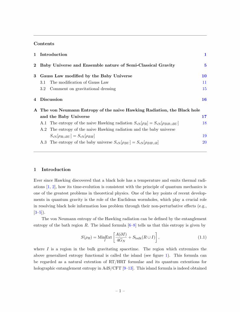
Figure 1: The Penrose diagram of the AdS black hole attached to the non-gravitating heat

bath. We take the radiation region R (violet solid line) in the heat bath. After the Page

time, the island region I (blue solid line) becomes non-empty, and the black hole region BH

(orange solid line) is outside the horizon of the black hole. The entanglement wedge of the

Hawking radiation R is the union of the domain of dependence of the radiation R and island

I regions (violet and blue shaded regions), and that of the black hole BH is the domain of

dependence of the black hole region (orange shaded region).

The island formula suggests that the entanglement wedge of the Hawking radiation con-

tains not only the radiation region R, but also the island region I. On the other hand, the

entanglement wedge of the black hole is its compliment (see figure 1 again). The bound-

ary of the island region ∂I is located just behind the horizon for an evaporating black hole

[6–8, 78, 79]. However for an eternal black hole, it is located outside the horizon [78–82].

In a recent interesting paper [83], such a form of entanglement wedge disconnected from

the asymptotic boundary is argued to be inconsistent with the long range nature of gravita-

tional force or equivalently diffeomorphism invariance. Let us consider a small local operation

on the island I which corresponds to a local excitation of on the radiation Hilbert space HR.

In a theory of gravity, such a small operation seems to be detected on the asymptotic bound-

ary of the spacetime using the gravitational Gauss law. This is problematic because the

asymptotic boundary belongs to the entanglement wedge of the black hole, see figure 2. This

implies that the local operation on the island region I (which is supposed to be a operation

on HR) can actually change the entanglement wedge of the black hole.

The above apparent inconsistency of the gravitational Gauss law is related to the in-

– 2 –

<latexit sha1_base64="FTNcIPZdLabAyX53WWzE7wyQ+x8=">AAAPS3icpVdbb9s2FHa7dWu0JU23x70wiwPEmGRYzq2F4aFLd2mAAsvUpingGAFF0TYRSjQoOkFi5J/s1+x12w/Y79jbMAw71M2SLLstIjSpQp7Ld875zqHojjkLVav11737H3384JNPH64Yn32+uvZo/fEXb0IxkYSeEMGFfOvikHIW0BPFFKdvx5Ji3+X01L14rvdPL6kMmQheq+sx7ft4GLABI1jB0vnj1b0zlw5ZMFXs4mbMiJpIetsLCea022ru9Q3D2LJKz8+SgQbm5XXDWDkjQkgPNhVF21w1EFZo29o1dxsdhFB53832LS1Q2paJ+gJt6abbWtlYKRsnifEnZktvF3WTzWRvTtnBHnMgLSJ4mUJs7pl2c7+ByqZmok6CJydprMC/re+8V+jwBTqmgRQhRR7DQ4l9sONJfBWnybKidHSyRZksSjeJTS/3PEqEBLdm8gJeuzdseIOH/ZkdUO28n4Jb6UMoRT1TjRi5yFt1c1aLIjIXQJTLrUOsRuj5j6/nYyTLYiUzV7EdndwINIpTnAK4ZIJTlQIYc6FQL/SFUCMTKRpotnftPprVKUTT2Pl2Xf+3AdTeKFT5m+1Wc8eEn0a9Uar/bedubmXsVs67dRpW5Naa9+vEfoue+zP4BxX4bcDf1nYC4dEedsUl7aOpU8bfn6E5qIBjazgLzEBJfggUDoac+jRQ6JR6Q4rEAKkRRbNiyapiiTEmTF13tYcB4zwORjWKcWzo+OoxDwpVsCwt7i4RT7m12Gq5kJWQZFHZgb9kBSQngSTdJeIyg7TIamd+vDoUBj/B6FRIfwQ43zVmQx9z/mrEBsm8jIg8N/KOQo4DLx1nbbO9QCKZYolAhYid2KhnJq08hHqlXdspKjlA2JKSkc6DXtRfpvVtPzoa9tMUJs6Btu2N1CjQHkhv52vr8gnNNHMUntaP6rfpsI8kYz+JfGJdu0psx3xHBcJf5QnPolBm9rSlKk7lTOej2MuigLYz2/EIAE6l+Vosr5t919Q9GlGwWsRKZbShDEScgBzn4GDymqI5QCyIghLJ4Y5CCIQq5tMC9eJI4SgJhvRDB2HKnjLk0hyDgrb2Ksfw3b07M+9OxThe4N2Z995fGkV5eB6+AP1q9SoYlepGiYqF2etyTC6QnhalJFXQsTRW31kOy44aDGWtkU7jpVo5pfxW5wPgFXtgUb3m4Dl5eIu0KuHpnoeW/0niS6aiowz64HtJw5AFw7TLh5LSICafqb+60RXz1Agi2PX992PjtJC7g6xnAc9daZqd7PvLvjNmYjvLxLJpqSvTI9c46L+nJmGScIp6EiQmYXd/DB8dEaNdysVV1262zYixMJSPz51kLG+9FHDtQGJM4w/V1LGkXqnbCimr8NUx4LqAkq/LhYoaEMp6rH42HrHt4/Ojhoaj9eNf+lwyzmjgFW5I5+ubUIDoQfMvdvKyWUue4/P1/848QSa6cwnHYdjT1ky7NVamC8SgsrsD9JmG0OAe5iKgt8bZJKTQHhd4SKfYD8Nr371FWz58WoflPb1YtdebqMGT/pQF4wlQkYAI7A0mHCmB9G0Q7iKSEsWv9aWESKYYQWSEJSYK7oyRJY2TM1dieT2dXSLC3IUibI7Bry8kJDAY3s5pQVFJnLCn0YPil4Pd5OWpnSXsTbtp7zd3f2lvPjtMUvew9lXt69p2za4d1J7VXtSOayc1svrr6m+rv6/+sfbn2t9r/6z9G4vev5fofFkrPI8e/A+vwHqi</latexit>

R R

I

BH BH

PR

�(PI)

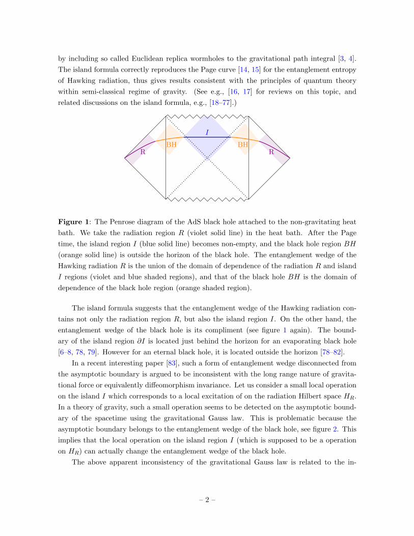
Figure 2: The Penrose diagram of the AdS black hole attached to the non-gravitating heat

bath with a small local operation φ(PI) (PI ∈ I, red dot) in the island region I. The

entanglement wedge of the black hole BH (orange shaded region) includes the asymptotic

AdS boundary. The gravitational Wilson line W (PI , PR) (green line) connecting two points

PI and PR (PR ∈ R, cyan dot) intersects the entanglement wedge of the black hole (orange

shaded region).

consistency of the gravitational dressing of local operators on the island region [83]. In a

theory with diffeomorphism invariance, a local operator can not be physical since it is not

gauge invariant. Instead, such a local operator φ(P ) needs to be “gravitationally dressed”

[84, 85] by attaching a Wilson line W (P, PB) connecting the point P to a point PB on the

asymptotic boundary. Then the resulting operator φ(P )W (P, PB) is gauge invariant. For

the gravitational dressing for a local operator on the island region PI ∈ I, which is a part

of the entanglement wedge of the Hawking radiation, it is natural to choose a point on the

bath region R as the asymptotic boundary point PR ∈ R. In such a case, the Wilson line

W (PI , PR) connects the two points is intersecting with the entanglement wedge of the black

hole. However the dressed operator φ(PI)W (PI , PR) should belong only to the entanglement

wedge of the Hawking radiation, thus this is problematic again. See the figure 2 again.

In this paper, we address the above paradox by carefully examining how the effects of

random fluctuations of an evaporating black hole is geometrized in a semi-classical description

of gravity. In principle the black hole evaporation process is described by the bipartite

system of the Hilbert space of the black hole HBH and the one for the Hawking radiation

HR. Of course, the description of such an entangled state involves a quantum theory of

gravity, therefore it seems impossible to study such a system efficiently. However, as was first

observed by Page [14], one can obtain a time evolution of the radiation entropy consistent with

– 3 –

unitarity, by averaging the entropy over the random fluctuations in the entangled state. This

opens up a possibility of having a partially fine-grained description of the evaporating black

hole while maintaining its semi-classical nature, to the extent of getting results consistent

with the principles of quantum theory. Indeed, in this way, the island formula makes it

possible to recover the Page curve in a semi-classical way. Specifically, the Euclidean replica

wormholes nicely capture the effects of these random fluctuations and their averaging through

a geometric way.

This paper concerns a description of these random fluctuations in a Lorentzian spacetime

in the semi-classical regime. We argue that the averaging over the random fluctuations can

be purified by introducing an auxiliary system, often called a baby universe. This new piece

of the spacetime is connected to the original spacetime with the black hole by an Einstein-

Rosen bridge, can be thought of as accommodating partially fine-grained information of the

evaporating black hole (see figure 4). See also [86, 87] for discussions on the role of baby

universes in the information loss paradox.

Motivated by this observation, we then study the gravitational Gauss law in the presence

of the baby universe sector. Such an introduction of the baby universe significantly modifies

the form of the gravitational Gauss law. For instance, assuming the baby universe part has an

asymptotic boundary, the gravitational Gauss law does not exactly hold within the original

spacetime as there is a contribution from the baby universe sector. This makes sense, because

restricting our attention only to the original black hole spacetime corresponds to a coarse-

graining. This is clearly seen from a Schwarzschild black hole solution, which has the horizon

area and therefore the Bekenstein-Hawking entropy SBH . However it is just one solution,

showing no degeneracy of the states, contradicting the huge degeneracy given by the entropy

eSBH . What we expect is that in full quantum gravity, one obtains microstates of the black

hole and by counting its degeneracy, one obtains eSBH . However after coarse-graining, all

the details of the microstates are lost, and one cannot see the microstate differences in the

Schwarzschild solution. Assuming the dynamics of the black hole is sufficiently chaotic, two

distinct energy eigenstates can never have the same energy, and the minimal value of the

difference is of order e−SBH . Thus the geometric description of such a class of microstates

by a single black hole space-time inevitably involves a coarse-graining, in which the energy

differences of order e−SBH are neglected. This suggests that in the black hole spacetime, one

can only trust the gravitational Gauss law up to O(e−SBH ) corrections.

The introduction of the baby universe with an asymptotic boundary naturally resolves the

paradox of the gravitational dressing as well, because the gravitational Wilson line starting

from the island region can now end on the boundary of the baby universe. This is a kind of

an expected result because the island region corresponds to fine-grained information of the

evaporating black hole, so can not have a simple description within the original black hole

– 4 –

spacetime.

The rest of the paper is organized as follows. In section 2, we study wormholes, and

the baby universe. In section 3, we present our main idea and explain how we modify the

gravitational Gauss law in the presence of the baby universe. We also comment on how the

boundary of the baby universe can resolve the gravitational dressing paradox. In appendix

A, we give the calculation of the von Neumann entropy of the Hawking radiation and that of

the Hawking radiation plus the baby universe in our formalism.

Note added: During the preparation of this paper, the papers [88–90] appeared, and

discussed extra information coming from the ensemble nature of gravity, which is related the

baby universe degrees of freedom in our paper.

2 Baby Universe and Ensemble nature of Semi-Classical Gravity

In this section, we clarify the role of the baby universe in the computation of the fine-grained

entropy of Hawking radiation through the island formula.

To this end, it is appropriate to begin with the fact that there are two distinct descriptions

of a theory of gravity. The first one is the fine-grained description, and the second one is

the coarse-grained one. In the first full-fledged fine-grained description of quantum gravity,

we have a sufficient number of observables (i.e., the complete set of operators of quantum

gravity) to perfectly distinguish quantum states. Note that, in the description, we can perform

measurements with arbitrary precision. We are interested in the gravitational system where

a black hole keeps emitting Hawking radiations. In a full-fledged fine-grained microscopic

description, an actual state in such a system has the following form,

|ΨM 〉 =N∑i=1

k∑α=1

FMiα |ψi〉BH |α〉R , (2.1)

where FMiα takes a fixed number. Here we define the orthonormal bases |ψi〉BH and |α〉R of

the Hilbert space HBH for microstates for the black hole and the similar Hilbert space HR

for the Hawking quanta participating in the entanglement. N and k are their dimensions.

The second description of the system is the coarse-grained one in terms of a semi-classical

theory, where we have a restricted number of observables, i.e., a subset of the complete

set of observables of quantum gravity, or coarse-grained observables like thermodynamical

quantities. The spatial and time resolution of such an observables is much larger than the

Planck scale. In this description, even by measuring coarse-grained observables precisely, we

cannot completely distinguish the underlying full quantum states of the full theory, but at

best a set of states with the same expectation values of the coarse-grained observables and

the same semi-classical geometries.

– 5 –

Owing to the restricted number of observables and also to the fact that the resolution is

much larger than the Planck scale, one is forced to describe the system in a coarse-grained

way, in terms of a mixed state, i.e., an ensemble of states {pM , |ΨM 〉}M . This ensemble

consists of the class of the states |ΨM 〉 with the random coefficient matrix CMiα

|ΨM 〉 =

N∑i=1

k∑α=1

CMiα |ψi〉BH |α〉R . (2.2)

From the semi-classical gravity point of view, two such states |ΨM 〉, |ΨN 〉 with different

random coefficients CM , CN can not be distinguished. This corresponds that a coarse-grained

observer describes the state in terms of the following mixed state,

ρBH∪R =∑M

pM |ΨM 〉〈ΨM | , (2.3)

where pM is the Gaussian probability distribution determined by the ensemble of states or

random coefficient matrix CMiα as

pM =

(Nkπ

)Nkexp

(−Nk tr(CMCM†)

), (2.4)

and satisfies∑

M pM = 1. See (A.1)-(A.3) in appendix A. We also note that the coefficients

Ciα are satisfying the following relationship,

〈1〉 = 1

〈CiαC†βj〉 =1

kNδijδαβ

〈CiαC†βjCkγC†δl〉 =

1

(kN )2(δijδαβ · δklδγδ + δilδαδ · δjkδβγ)

〈(Πna=1Ciaαa)(Πn

b=1C†βbjb

)〉 =1

(kN )n(all possible contractions of indices)

〈(Πna=1Ciaαa)(Πm

b=1C†βbjb

)〉 = 0 for m 6= n

(2.5)

where 〈·〉 means the average over the random coefficient matrix CMiα . Randomness of the

coefficient in (2.2) is due to the fact that the dynamics of a black hole is highly chaotic. These

can be understood as follows: Suppose that an observer tries to experimentally specify the

fine-grained state (2.1). Then the observer needs to perform a measurement with the Planck

scale precision. However, for coarse-grained observers, the resolution of the measurement

is much larger than the Planck scale. Note that during the measurement time-scale, the

microscopic state can evolve. Therefore, if the measurement time-scale is much larger than

the Planck scale, the microscopic state can evolve to almost all states of the form (2.2). In this

way, coarse-grained observers see the black hole state as (2.2). This provides an intuitive way

– 6 –

to understand the reason why the random matrices appear in the semi-classical description

of the black hole dynamics.

Once we coarse-grain the system, the state is reduced from the pure state (2.1) to the

mixed state (2.2), and apparently we lose the microscopic details of the states. However we

nevertheless can compute some aspects of the fine-grained entropy of Hawking radiation by

purifying this mixed state by introducing an auxiliary system HBU , which we often call the

baby universe. For instance, recent progress in understanding the island formula suggests

that the purification enables us to capture some part of fine-grained information of Hawking

radiation while maintaining the semi-classical description. Discussions on the relevance of

random fluctuations for physics of black holes can be found for example in [91–93]. We also

note that Gaussian random fluctuations have a geometric interpretation in terms of end of

the world branes in two-dimensional JT gravity [3].

Note that to purify the original system with the mixed state (2.3), we need an auxiliary

system HBU whose dimension is at least equal to or greater than that of the original system.

The dimension of the baby universe Hilbert space depends in particular on the coarse-graining

procedure. On this new Hilbert space, the simplest purified state is given by

|Φ〉BH∪R∪BU =∑M

√pM |ΨM 〉BH∪R|M〉BU , (2.6)

where {|M〉BU} are orthonormal baby universe states. A fine-grained observer can access

to this auxiliary system, but coarse-grain observers can not. Let us emphasize that the

description using the auxiliary system is not a full fledged fine-grained description of the

system. This is because we are artificially adding degrees of freedom, which do not show up

in the original Hilbert space HBH⊗HR. More concretely, in the quantum gravity description,

the actual fine-grained state realized in the system is one of the states in the ensemble, not the

one with the baby universe. We nevertheless consider the purified state (2.6), because it has

an effective semi-classical description, on the contrary to the full fledged fine-grained state in

quantum gravity. Furthermore, as we will show later, if we are only concerned with averaged

property of the fine-grained entropy, such as the Page curve, considering this purified state is

good enough.

Note that by tracing out the black hole degrees of freedom BH in the mixed state (2.3),

the reduced density matrix of the Hawking radiation ρR gives an approximately thermal

mixed state, and the von Neumann entropy SvN[ρR] gives the Hawking’s result

SvN[ρR] = SvN[ 〈ρ(M)R〉M ]

= log k,(2.7)

where we have defined,

ρ(M)R = trBH [ |ΨM 〉〈ΨM |BH∪R ] , 〈ρ(M)R〉M =∑M

pM ρ(M)R. (2.8)

– 7 –

See the appendix A.1 for detailed derivation.

Now let us consider the same entropy of Hawking radiation in the fine-grained descrip-

tion. To do so, let us first figure out a geometric description of the purified state (2.6). In this

state, the Hawking radiation HR and the black hole HBH are entangled with the auxiliary

baby universe HBU . From the viewpoint of ER=EPR [94], we expect that this is realized geo-

metrically by an Einstein-Rosen bridge connecting the baby universe and the original system

(see figure 4). The property of the ER bridge depends highly on the choice of the ensemble. If

we realize this system with in the framework of the AdS/CFT correspondence, the auxiliary

universe can be modeled by an additional boundary and its gravity dual involves an Einstein-

Rosen bridge connecting the new boundary. This purification process is the key in recent

studies, especially in the finding of the island formula which captures some aspects of fine-

grained information of the quantum gravity states, in the semi-classical description through

a non-perturbative way. For instance, in describing an evaporation process of a black hole

semi-classically, such non-perturbative contributions are required to get a consistent result.

In such a process discreteness of energy spectrum of the black hole microstates is a crucial

ingredient to ensure unitarity of the process. However, in the coarse-grained description, en-

ergy differences between black hole micro-states are invisible, since they are typically of order

O(e−SBH ), where SBH is the Bekenstein-Hawking entropy [95]. A discrete energy spectrum is

only after including non-perturbatively small contributions which are provided by Euclidean

wormholes [96, 97].

What the island formula implies is that one should identify the fine-grained Hilbert space

of the Hawking radiation HR with the tensor product of two Hilbert spaces HR⊗HBU , after

the Page time. On the other hand, before the Page time HR should be identified with just that

of the Hawking radiation HR, and correspondingly the Hilbert space of the black hole should

coincide with the tensor product of the black hole and the baby universe HBH ⊗HBU . This

difference between the radiation Hilbert spaces before and after the Page time comes from the

fact that the inequality for the dimensions of the Hilbert spaces of the Hawking radiation and

that of the black hole changes. In fact, before the Page time, since the total state (2.6) is pure,

the von Neumann entropy of the union of the black hole and the baby universe BH ∪BU is

equal to the previous von Neumann entropy (2.7) of R, i.e., SvN[ρBH∪BU ] = SvN[ρR] = log k,

which is consistent with the island formula before the Page time.

After the Page time, the reduced density matrix of the Hawking radiation and the baby

universe ρR∪BU in (2.6) gives the the fined grained entropy of the Hawking radiation, which

deviates from the entropy (2.7) of the naive density matrix (2.3),

SvN[ρR] = SvN[ρR∪BU ]

= logN

= SBH .

(2.9)

– 8 –

In appendix A.2 we provide details of this calculation. The result reproduces the behaviour of

the Page curve after the Page time, giving the Bekenstein-Hawking entropy SBH . Therefore

by appropriately dividing the total system BH ∪ R ∪ BU , we can get the von Neumann

entropy which obeys the Page curve (see table 1)1.

Black Hole Hawking Radiation von Neumann Entropy

Before the Page time BH ∪BU R SvN[ρBH∪BU ] = SvN[ρR] = log k

After the Page time BH R ∪BU SvN[ρBH ] = SvN[ρR∪BU ] = SBH

Table 1: How to divide the total system BH ∪R∪BU into two sub systems before and after

the Page time, and the corresponding von Neumann entropies.

At the same time, we know that the fine-grained entropy SvN[ρR] of Hawking radiation

is computed by the island formula (1.1) too. In the entropy calculations using this formula,

it was crucial to include the contribution of the island, which typically occupies the region

behind the horizon of the black holes. Therefore it is natural to identify the island region

behind the horizon with the Einstein-Rosen bridge of the purified state (2.6) connecting the

original spacetime and the baby universe, which stores fine-grained information of the original

spacetime.

These states {|M〉BU} in the fine-grained Hilbert space can be naturally identified with

so called α states [98–100] in the baby universe Hilbert space which diagonalizes the boundary

creation operators [87]. Then each fine-grained state |ΨM 〉|M〉 belongs to different superse-

lection sector, because each α state does. In particular, this means that off diagonal element

of matrix 〈ΨM |〈M |(O ⊗ I)|ΨN 〉|N〉 for any local operator O on the black hole BH and the

Hawking radiation R vanishes, therefore any local measurement on them can not distinguish

the entangled pure state (2.6) with the mixed state only with classical correlation of the

1One may also consider the possibility of dividing the baby universe Hilbert space HBU into two parts

HBUBH ⊗HBUR , and then define the radiation Hilbert space as HR = HBUR ⊗HR, instead of HR = HBU ⊗HR which we do in the body of the paper. In such a case, the states of the baby universe are given by

|M〉BUBH ⊗ |M〉BUR . In this case, assuming the orthogonality of the basis of HBUBH , we see that the entropy

of ρBUR∪R is given by

S(ρBUR∪R) = −∑M

pM log pM +∑M

pMSvN (ρM ), (2.10)

where ρM is the reduced density matrix obtained by tracing out HBUBH ⊗HBH in (2.6). Then it is natural to

define the fine grained entropy of Hawking radiation S(ρR) as a conditional entropy of knowing the probability

distribution pM by subtracting the classical Shannon piece H(pM ) = −∑

M pM log pM

S(ρR) = S(ρBUR∪R)−H(pM ) =∑M

pM SvN (ρM ). (2.11)

However we do not know the natural choice for such a splitting of the baby universe Hilbert space HBU .

– 9 –

following form

ρ =∑M

pM |ΨM 〉〈ΨM | ⊗ |M〉〈M |, (2.12)

in the sense that

tr [|Φ〉〈Φ| (O ⊗ I)] = tr [ρ (O ⊗ I)] =∑M

pM 〈ΨM |O|ΨM 〉. (2.13)

In other words, LOCCs acting only on the the black hole BH and the Hawking radiation

R, which can be available to coarse-grained observers, can not distinguish the classically

and quantum mechanically correlated states (2.6), (2.12). However one can easily see the

entanglement entropy of these two states on R = R ∪ BU are different. Indeed, the entropy

of ρ contains a classical Shannon term, whereas the same entropy of (2.6) does not. From

another point of view, LOCCs on the sub-system BH ∪R and the baby universe BU , which

can only be available to fine-grained observers, can distinguish the classically and quantum

mechanically correlated states, since the equalities in (2.13) does not necessarily hold for

operators on BH ∪R ∪BU .

In the next section, we discuss several properties of the baby universe and the wormhole

connecting the baby universe and the original spacetime. The wormholes may be dependent

on the actual geometry of the baby universe. We cannot fully specify the geometry of the

baby universe from the first principles of quantum gravity. There is a canonical and minimal

choice for such a baby universe; starting from the original system |ΨM 〉, we prepare a copy of

it |ΨM 〉, and regard it as a purifier |M〉BU = |ΨM 〉Puri.. Then the expression (2.6) becomes∑M

√pM |ΨM 〉BH∪R|ΨM 〉Puri.. (2.14)

The existence of the boundaries in the original system |ΨM 〉 implies that purifier |M〉BU =

|ΨM 〉Puri. should also have boundaries. More generally, there is a possibility that we may

choose the multiple copies of the original system as the baby universe |M〉BU = |ΨM 〉⊗nPuri.

and further choose their linear combinations as that. Again from ER=EPR this entanglement

between the two spacetime implies the existence of the wormhole connecting two island regions

for two spacetimes. This wormhole will affect the non-perturbative physics of this system.

Note that the more the number of copy of the original spacetime increase, the more the effects

from wormholes are topologically suppressed.

3 Gauss Law modified by the Baby Universe

In this section, we discuss the physical consequences of the existence of the baby universe

sector introduced in the last section, which accommodates fine-grained information of the

system. We are mainly interested in how the baby universe helps to recover information of

– 10 –

the black hole interior from Hawking radiation. We will also briefly mention the relation

between our discussion and the paradox raised in the recent paper [83].

Before doing so, let us present a remark. In the light of AdS/CFT correspondence,

the introduction of an additional boundary, i.e., the boundary of the baby universe sounds

puzzling, because AdS/CFT is the correspondence between a theory of full quantum gravity

in the bulk and a (non gravitating) CFT on the boundary. This means that in principle, all

the details of the bulk quantum gravity Hilbert space can be read off from the single CFT

Hilbert space. Therefore, we do not need the second copy of the CFT, as we did in the

previous section, which results in the baby universe sector.

Nevertheless, we are forced to do so, because we are sticking to a semi-classical description

of the system. Then, to restore fine-grained information within the semi-classical regime, we

need to introduce an auxiliary system and regard the new degrees of freedom as a part of

the radiation degrees of freedom after the Page time. If we do not do this, this restriction

amounts to that on the boundary, we are only accessible to a sub-Hilbert space Hcoarse which

characterizes coarse-grained degrees of freedom. To incorporate the rest of the CFT Hilbert

space, which we term Hfine just because it describes fine-grained degrees of freedom, we need

to introduce a second copy of the CFT Hilbert space, and accommodate Hfine to it.

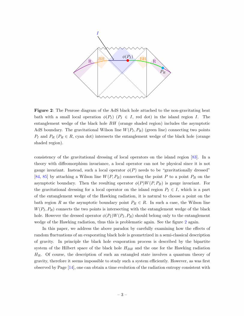
The full Hilbert space on the single boundary is obtained by gluing two asymptotic

boundaries of the spacetime. In the resulting bulk spacetime, there are two homologically

inequivalent paths, both of which connect a point in the interior of the black hole (and

belongs to the island region) to the boundary of the spacetime (see figure 3). The first

path is the trivial one (the blue line in figure 3 ), which entirely lies within the original

spacetime. This path necessarily intersects with the entanglement wedge of the black hole.

However, in the presence of the baby universe, there is a second path which does not cross

the entanglement wedge of the black hole. Instead, it crosses the Einstein-Rosen bridge

connecting the original spacetime to the baby universe, and reaches the second asymptotic

boundary which accommodates fine-grained degrees of freedom as in the green line in figure

3. Since these two boundaries are in the end glued together, it connects the island region and

the conformal boundary, without passing through the entanglement wedge of the black hole.

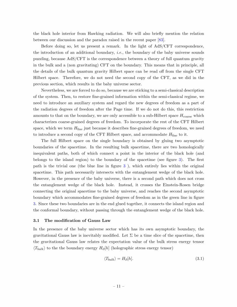
3.1 The modification of Gauss Law

In the presence of the baby universe sector which has its own asymptotic boundary, the

gravitational Gauss law is inevitably modified. Let Σ be a time slice of the spacetime, then

the gravitational Gauss law relates the expectation value of the bulk stress energy tensor

〈Tbulk〉 to the the boundary energy H∂ [h] (holographic stress energy tensor)

〈Tbulk〉 = H∂ [h]. (3.1)

– 11 –

<latexit sha1_base64="31/4hPt0JeNxQWqQShlnkSq+vLY=">AAAf/3ic5VndbttGFla6bbdWf7O9LAxPNjJgIaQgMrKTwHXROmibAAHWy8RNAVkISGokEaZIYTiKqwi66GWfZO8Wve19X6KvsLfdB9gzwyE5Qw5lOUlbFCvYMM05/+fMN+eMvFkYJLTb/eXaG3958623//rOVvPd997/4MOPrv/tmySeEx+f+nEYk289N8FhEOFTGtAQfzsj2J16IX7qnd9n60+fY5IEcfSELmZ4MHXHUTAKfJfCq2fXtwdnHh4H0ZIG5y9mgU/nBK/6ie+G+Kjb2R80m81ds/T5BwmAww3L75vNrTM/jskQFilGeyFtI5eiPbNn9NqHCKHyupevm4ygtEwEew038bJlxtzcKgv3hfC7Rpctq7xiUaxVmB13GDgQljh6lJnY2TeszkEblUUVpI6wR6JsbsHP7hfDx+j4ATrBEYkTjIaBOybuFOQMiXuRhsk0eTgO85dEvCSe8I297g+xHxNQa4gH0Hr0Ihi/cMeDQg6wHm7G4Gl1xJTioUEngX8uS/UkqSoJkRzgsdw9dukE3f/qSdVHf52vfqEqlcOCy41GaYgzA54HcYhpZsAsjCnqJ9M4phMDURyxaj+yBqjIU4KWqfK9FvtzA0r7hpLlW3vdzm0Dftutdin/q8NXU0tStaSq1mmbXK1Z1eukelXNg83Mj+Ih7rte/BwP0NIpmz/Y0JiqFEjIlxF1o3GIpzii6CkejjGKR4hOMCpSRXSpimeuH9AFYIpljIIwTF2hbdWNG8y7VloFSg5Mk5F7a8izyqqXWk6j1iSiMjvwH9GY5AiTiLeGnOQm1Uk9rIKrgwH2fRc9jcl0AnZeBrLJ1A3Dx5NgJNCS10EF8B4moRsNMzCzDbuGQmCYINCQWEJGKxdpyia0tHItR2VyoF5LTFluvHCOBxklKEurVAhRq3LZethaZejNmfnGNIQIIYAlQLCnJYyUGr6Qazjg1hXymCRdmUii9YbCTjLsdBtBmWQhqKdn27cHMW+1eVXpScyMhgnKjUgDIJURnDTDTtwZoSDiTsXitEYJOIJpMMVKNaWewtkQjfFVkS0riLLJJWQCXOrua3H11bU7hXZHA2k12p2q9mrRycaW8fD4AfDr2XVmaNmbpVJU4NQLXf8cMQAoBUlTjiWkvDQdptWxMozKUlituzKXxCQvHV7BPHUP1OWrYp4jm1fHpTXPSRsJ9lMB2vvxbGFX0LWMeUmBrNYBdHZdXatJ7Qzf4Oy5JXha+pa3IPUU0krzmxOSS2SSQiZRZGp64pySt8UKbalBzikrhOu65ZxLrZ6Me133rGF1Sqyb9NJ21mDaSodpZ61lerDtos066oyNMrYNmbySrrq+WiWr6axld7ZSw4vuOjNI9ttXAlBQFCHwZcXF6VknBKHMXdSX/F2mDq8AzWBzKk6v8qeSQib/cmGy21RI8xd+iA/rZgK5ojzXW5jfZb3QvqYX4hQLQQGnQ68IPyliv/lQYYupwq4Cp5035j1+ArXKi8LaW5lRLXnceAlriLCGaKyBHZZ3+FVz+Oo6c9Y6aYGLd9RjzgDzIZ+t49OWIqPGNOhvLhUig/iTGDZ/QoNoPA+SCaIXcV2Dw46hvnwucZl/hnLXnFr/p+OBTpdd0ZWdFhvotHU6Ob1Gd3NXlK+YMMzPBuze6aDabd2VW3ooZysd8tThhnNWBxkJrK8y/mjmJltmtF/H3FRDZxd0tui18lDx4eklBwoGzIBS+xyjxKPUCuQZXEFXsPsaVDpMJYPpVKOZPlY0Pko18sAxVEH9rwnGkYEKdLEH0J7lY6D5mzne3MoDz7v3qyiyH9V4mcegCAtXlJ++r3PMNNJe54+dNl/OiFcaOtUw5p8TaOoqWC5vO3bDjy6CIZ0c3TZO4J+09tY7AIhUcaEWXADXoYDb7Fo8r0F+KKs1KGOMJWMMI09vv+/JDNmkXMjlYOThML446hWuDJYsBsjmQar1nO/xq2RtqTh8R3b4VdOZX6QerLtIRVIEFHYlDBxV0whYK829IGt58HcUlWsk6909Rd4+tBbZ1zTocbYjCzt4t1KiP4aeD51GAfu6CE7JkzkJRgEm7ZW2ETHNh0Mc0fyrJK1d/U/Nz9YDsr5A9felrM1kvWtXFFs9HeTZYFRpMjdozvntGgwLnQPguiXGgtZmjT3nZVvnHnAUIf5d7FNulb6GEipg7tLQW+ywqoRef3vOKvqAowPfNq2NCDPv1g4jwjvLsDkP862X7porcuaR/33MkxuqLPDNMxwNlW9Sn310E6CDf1D1wRIPNxvic/Ls+rUfzoaxP2c3gn7oJkmfiTOs7owaHqQKk6Pb06kxfB7Mksid4mSwTCj0r24YR3jVPJsnGHb7uTvGS3eaJIupt0K7U0CVpLzGXurW+nM6ujtYBtFsDpXiAwmsjeYhojFi3yDD2EWwT8MFu3zxSUADH/kTl7g+BeBoKmqY7alR7CkMPOKSxbKYhBLpBiXpzMCUaUxmExjqqly+G/rVt8nEneGkM8bxFFMSAEWFBMSCZVGiRmc2HrFtkaxKFkNzAB0MgfCnybvHPyh9uNMTD/esPHnf2B3roNP7p33z82ORxncanzT+3thrWI07jc8bDxonjdOGv/3z9n+2f93+7873O//a+ffOjynpG9cEz8cN5bPz0/8AtLtOdQ==</latexit>

R R

IBH BH BU BUI

Path 2

Path 1

Original Spacetime Baby Universe (Purifier)

Glue

Glue

Figure 3: Schematic picture of the geometry of the AdS black hole coupled the bath CFT

(left Penrose diagram) and the baby universe geometry (right red Penrose diagram) connected

by the Einstein-Rosen bridge (transparent green shaded region), corresponding to the state

(2.14). After the Page time, the fine-grained Hawking radiation R is the union of the Hawking

radiation R (violet region) and the baby universe BU (red region). We regard the above

spacetime describing this union by gluing two distinct asymptotic boundary regions BU and

R . The island region I is connected to the fine-grained Hawking radiation R∪BU thorough

two paths, path 1 and 2. The path 1 (thick blue dotted line) intersects with the entanglement

wedge of the black hole BH (orange shaded region), but the path 2 (thick green dotted line)

does not intersect with that.

Here the boundary energy H∂ [h] is explicitly given by the integration of the ADM current J i

over the conformal boundary ∂Σ [101],

H∂ [h] ≡ 1

2κ2

∫∂Σdd−1x

√g niJ

i (κ =√

8πGN ), (3.2)

where ni is the normal vector to the boundary ∂Σ, and the ADM current J i is defined by

Ji ≡ N∇j(hij − hg0

ij

)−∇jN

(hij − hg0

ij

)(3.3)

under the ADM decomposition

ds2 = −N2dt2 + gij(dxi +N idt

) (dxj +N jdt

), (3.4)

and the expansion from the background metric gij = g0ij + κhij . More precisely, (3.1) is

a perturbative version of the gravitational Gauss law which can be derived from the full

Hamiltonian constraint

H[πij , gij ] = 2κ2g−1

(gijgklπ

ikπjl − 1

d− 1

(gijπ

ij)2)− 1

2κ2(R− 2Λ) +Hmatter = 0, (3.5)

– 12 –

where gij is the metric on the Cauchy slice, πij is the conjugate momentum, and Hmatter is the

matter Hamiltonian density. Expanding (3.5) from the background metric, gij = g0ij + κhij ,

then look at the second order of the expansion gives (3.1). Details of the derivation can be

found, for example in [101]. H∂ [h] should be understood as the change of the mass of the

black hole, H∂ [h] = MBH [g + h] −MBH [g] due to the back reaction from the bulk stress

energy tensor, 〈Tbulk〉.In the paper [83], it was argued that the gravitational Gauss law provides an interesting

puzzle on the island formula. Suppose we act a local operation on a state on the island region.

Since information of the island region is encoded in the Hilbert space of Hawking radiation

HR, this operation can be regarded as a local operation on HR. This operation changes the

expectation value of the bulk stress energy tensor. Then the gravitational Gauss law relates

this change of 〈Tbulk〉 on island region behind the horizon to the change of the boundary

energy H∂ . This means that any change on the island region, no matter how it is small,

is always detectable from the conformal boundary ∂Σ. However, this sounds troublesome

because ∂Σ belongs to the entanglement wedge of the black hole. For instance, this implies

that in the bipartite system HR ⊗ HBH , a local operation on HR can change the state of

HBH .

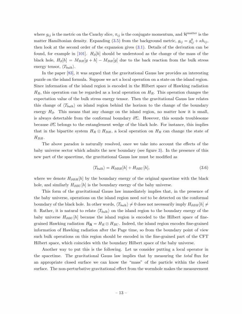
The above paradox is naturally resolved, once we take into account the effects of the

baby universe sector which admits the new boundary (see figure 3). In the presence of this

new part of the spacetime, the gravitational Gauss law must be modified as

〈Tbulk〉 = H∂BH [h] +H∂BU [h], (3.6)

where we denote H∂BH [h] by the boundary energy of the original spacetime with the black

hole, and similarly H∂BU [h] is the boundary energy of the baby universe.

This form of the gravitational Gauss law immediately implies that, in the presence of

the baby universe, operations on the island region need not to be detected on the conformal

boundary of the black hole. In other words, 〈Tbulk〉 6= 0 does not necessarily imply H∂BH [h] 6=0. Rather, it is natural to relate 〈Tbulk〉 on the island region to the boundary energy of the

baby universe H∂BU [h] because the island region is encoded to the Hilbert space of fine-

grained Hawking radiation HR = HR ⊗HBU . Indeed, the island region encodes fine-grained

information of Hawking radiation after the Page time, so from the boundary point of view

such bulk operations on this region should be encoded in the fine-grained part of the CFT

Hilbert space, which coincides with the boundary Hilbert space of the baby universe.

Another way to put this is the following. Let us consider putting a local operator in

the spacetime. The gravitational Gauss law implies that by measuring the total flux for

an appropriate closed surface we can know the “mass” of the particle within the closed

surface. The non-perturbative gravitational effect from the wormhole makes the measurement

– 13 –

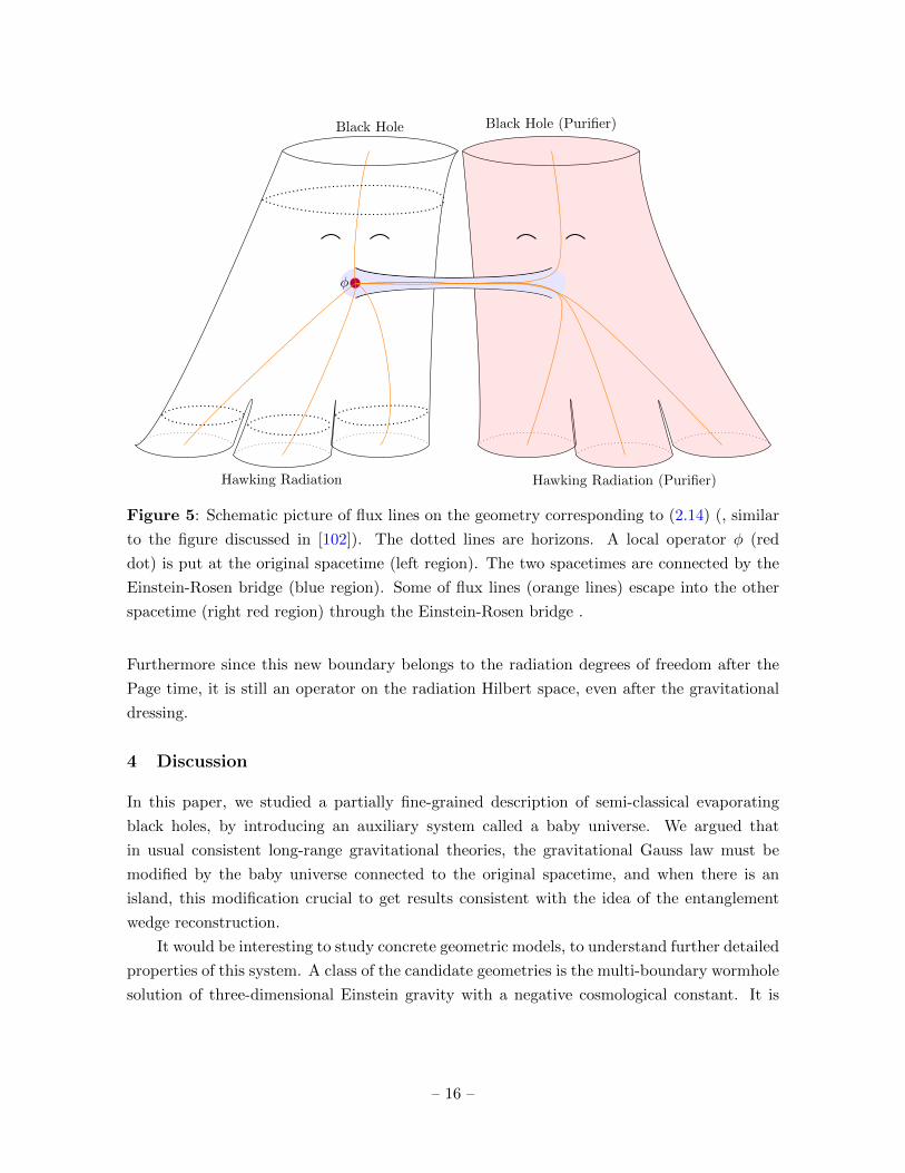
of the flux highly non-trivial. The wormhole can release some part of the flux of the original

spacetime into the purifier (see figure 5). Here we note that since in our setup the baby

universe has boundaries, flux lines can end on the boundaries of the baby universe as figure

5. Namely, in measuring the total flux, we also need to consider the purifier (right spacetime

of figure 5) or equivalently the baby universe in addition to the original spacetime (left

spacetime of figure 5). By the usual gravitational Gauss law, if we just measure the flux

of the original spacetime only (left spacetime of figure 5), then we cannot specify the exact

mass. The modification is not visible within the coarse-grained precision. However, without

the modification, we may encounter many problems, e.g., violation of the conservation law.

There are several other implications of the generalized Gauss law (3.6) as well. First, the

existence of the baby universe boundary energy term indicates that the gravitational Gauss

law does not precisely hold within the original black hole spacetime, 〈Tbulk〉 6= H∂BH [h] in

general. For instance, one way to think about the generalized Gauss law of the form (3.6) is,

it relates the spectrum of the fine-grained part of the spectrum H∂BU [h] to the coarse-grained

part H∂BU [h]. We expect that the fine-grained part is discrete, and the typical differences

between two nearest energy eigenvalues are of order e−SBH . This forces the coarse-grained

part also discrete, which is necessary for unitary time evolution.

Let us estimate the magnitude of the violation of the gravitational Gauss law in the black

hole space time. In order to obtain a unitary time evolution of an evaporating black hole,

we need non-perturbative effects of order e−SBH , where SBH is the entropy of the black hole.

This means that we need fine-grained states in a small energy window of order e−SBH , thus

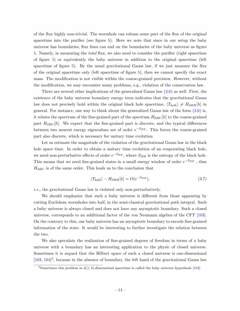
H∂BU is of the same order. This leads us to the conclusion that

〈Tbulk〉 −H∂BH [h] = O(e−SBH ), (3.7)

i.e., the gravitational Gauss law is violated only non-perturbatively.

We should emphasize that such a baby universe is different from those appearing by

cutting Euclidean wormholes into half, in the semi-classical gravitational path integral. Such

a baby universe is always closed and does not have any asymptotic boundary. Such a closed

universe, corresponds to an additional factor of the von Neumann algebra of the CFT [103].

On the contrary to this, our baby universe has an asymptotic boundary to encode fine-grained

information of the state. It would be interesting to further investigate the relation between

the two.

We also speculate the realization of fine-grained degrees of freedom in terms of a baby

universe with a boundary has an interesting application to the physic of closed universe.

Sometimes it is argued that the Hilbert space of such a closed universe is one-dimensional

[103, 104]2, because in the absence of boundary, the left hand of the gravitational Gauss law

2Sometimes this problem in d(≥ 4)-dimensional spacetime is called the baby universe hypothesis [104].

– 14 –

<latexit sha1_base64="3joTZ6QYXXapLo9pWTFrUdLJQJo=">AAAWkHic1VhZb9tGEFZ6xuqVw/BLXzaNDFgIKUiM7Tgw3CYO2iaFgbqMHQeQBGO5XEkL88Luyqki6K196E/sn+hv6CzvS7GMpA8lbIjgzsw3M7vzzZBW4DAhu92/b3z08Seffvb5zbXmF19+9fU3t27feSX8KSf0lPiOz19bWFCHefRUMunQ1wGn2LUcemZdPFPrZ5eUC+Z7J3IW0KGLxx4bMYIlPDq/ffefgUXHzJtLdvE2YEROOV30BcEOPeh2dobNZnNTL12/cgYa2Ck/bzbXBsT3uQ2LkqItR7YRlmhL39a22/sIofK6la7rSqC0zGP1JdrcSpaVcnOtbJzExve0rlou6saL8VpF2cQ2MyEtvneUuNjZ0Xqd3TYqm8pEzdifnGRzDf42n9ov0eFzdEw97guKbIbHHLtgx+b4TZQmXQ/TsZ8+5PFDbsWxqcd9mxKfA6wW3wDqwVs2fovHw8wOqO6vpmDVYvhSUluTE0Yu8latnNWiCM8FEOZy8xDLCXr200k1RvKuWEkGFdlRyQ2dRlGKEwcume9QmTgQOL5EfeH6vpxoSFJPnfaD3hBl+yTQPALfaqmfe3C07xV2+cFWt/NQg/92q13a/8X++8HyCJZXYc22HsLqVVwzwi0iD1dz3/Nt2seWf0mHaG6W3R+u6EzFSlQn6qdKCc/8YGZU+KBcVmLCRnFR93ahTLp1dSuNSKKlDs2DWKdVzx+ZqFUQrTBJKsivsMkzm7xgs4ZgUsmQYwqyJbZJJSuC76KeVKu404n2u6ioRtUsqa5CTEZSrUahXI2kTsPHzU20Gj0lalKprahklbCWkVRRbAlN5cNZixzPqCpxKB83KSQgk8hSQPLAa6mDy4wglISL+rl451HAC6g0XS8GvUjvSoDK/tXG8mHL2BqZEYeGG1fDsJtx8niWudX51YgJ1qhSlJFy1HaZYo2Q694DmMfAvAYYSiHltTKyGSEX+OzEhzoQknnjKRMTJN/4SASYUMlcWph1BiPmOH0f1picwazU08DzIfo/7HwNgZsUpk2C0ZnP3Qm0iatmO+Fix3mZ8Xm4tRXmeyEc7NnJDGVoxhKJeHSKBWpEekcJoSUm9bwLVc4NlcyiUsiAJaUaNaOClRDnCphGHWYoX4OdkEU/PO+a/v1QjbO70aa1ksDhRO/dSwKCIoIS6sXoYcFYzpQmirmmPW+9aKnDnbFW3uJOarFVp1U03UrykikayxQzjo6Cik3EyCqwGHd/qZyRyQFMxNRJppTYdekhOUBwShUL7IRcEd/memK6fwtoj5sfANJUkIrxIkQ9uq0gHkWIYeIUp8SIKKMWYwhjSmJT1/+zuJtrad6P1CG8DpDSqA0yTUGWlRAo60IZy8AwYnf8zggxD8kJRX78prmMgsPzA+znjeMd0qKef/2zUS6O0nANEXR3al8NPpgTZuaEWTOcL3HCrDoxXDmYwoh/+BwM1du5yp+qHWCdHz0JVhzqUk+iM2qPYTtH4a5aDiYXSHWZUvbyzVRVwrCU7jIt1oSm90JyRCnRhGpXaeWU8kv713DPLLi3LGMV98y8e8u0at1TDFqsnvT6GU8h2zanQsAcg8qtHEWjC5lhr3pWsq5AGIcKRX0OkFNxsBvI4T7ortBLUHoYWoNgwraO263skEYlMuaUessqBBpepUaWAsLUAAzZVh9zUpLTexWqzfewx/keBivbmpGXTeqgZik86UBKEwkN7/h8IOnvch5MOessomZbsxsnIFPZg9x3kax6DnYgZcnXNfQy4bzMn3CiK8kfYmuGTj2mvvLBEHIMzowY5e2wGQ+oZxc+7Z3fug9VG16oetOLb+434uv4/PaNvwa2T6aqjImDhegrc1qvG0jNgh2i/OCh62r2JQuEh10qhnMBhW9jx/foojmYCgpxXOAxnWNXiJlrLdCmCy9dorymHtat9adytDecMy+YwgEhIAJro6mDpI/UJ02Y1zkl0pmpF1jCmWQEkQnmmEhISbMAo3yPnFJ3DrM45rN5NkKL3Fuo6ATgiutzOMLeuKpFsEOqT8UEB1R0xtR3qeQMJCoiYBY880QxO8F4pKpBLEoeA/dA9+OQ/mjzHocXim4ebcc3j3vp5r0yOr3dzvZvxv0nh/E23mx82/iusdXoNR41njSeN44bpw2yfro+X/9j/c+NOxt7Gz9sPI1EP7oR69xtFK6NX/4FFwSiZg==</latexit>

R R

I

IBH BH�(P )Ppuri.

Original Spacetime Baby Universe (Purifier)

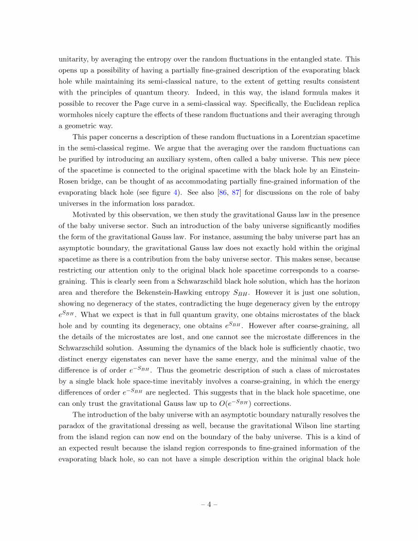
Figure 4: Schematic picture of the geometry of the AdS black hole coupled the bath CFT

(left Penrose diagram) and their copy (right Penrose diagram) connected to the original

spacetime through the wormhole (blue region), corresponding to the state (2.14). The local

operator φ in the island (cyan dot) can be gravitationally dressed with a gravitational Wilson

line Wgravity(P, Ppuri.) (green line) which ends on the baby universe (right Penrose diagram)

without intersecting the entanglement wedge of the original black hole degrees of freedom

(orange shaded region).

(3.1) is always zero, so any operations are not allowed at all. However, as we saw above, one

way to obtain its fine-grained description is to connect it to an open baby universe with a

boundary. Then the generalized Gauss law (3.6) does allow operations on the baby universe

boundary only. It would be interesting to explore further implications of the observation.

3.2 Comment on gravitational dressing

In a theory with dynamical gravity, a local operator is not physical, since it is not diffeo-

morphism invariant. One way to make it diffeomorphism invariant is to connect the lo-

cal point P to a point P∂ on the boundary, via a gravitational Wilson line, i.e., φ(P ) →φ(P )Wgravity(P, P∂). This prescription is called gravitational dressing. In [83] it was argued

that such a gravitational dressing of a local operator on the island region leads to a incon-

sistency of the island prescription. This is because the relevant gravitational Wilson line

connects a point on the island to a point on the conformal boundary of the AdS black hole.

However, this sounds puzzling, because whereas the island prescription asserts an operator

on the island region locally acts on the radiation Hilbert space, the gravitational Wilson line

attached to it enters the entanglement wedge of the black hole, thus it does change the state

of HBH .

In our point of view, the above paradox is naturally resolved, since in the presence of the

baby universe with a boundary, the gravitational Wilson line can end on this (see figure 4).

– 15 –

<latexit sha1_base64="IvVOe0MMyoQI+miZ6XKTsmb52HI=">AAAl0Xic7VpJb9tGFFbSLVa3pD32MqkkQIZJliIlJ4FhIEiRwgcbTdlmKWTBIKmRNDBFEuQoriIIKHoreu+v6bX9D/03Hc4MpeEimlrsU5lDqJnH+d42730c2vIdFGJV/ffO3ffe/+DDj+7tVT/+5NPPPr//4ItXoTcJbPjS9hwveGOZIXSQC19ihB34xg+gObYc+Nq6/Daaf/0WBiHy3J/w1Ie9sTl00QDZJiZDFw9q35xbcIjcGUaX73xk40kA593QNh143FK0XrXakBfXKRxg8L2NPX8SyoVX9dz2vKCPXBND0MT2PjAxaLaUx1J7/yg5adktNitrkqxlZzU2q5JJJWdaZ9P82RSu578JR2iAl/BqegUi87Mgo0qqotOF+oF5BXzHw6Abjj0PjySAoRs5kjim0wPLRUIwA816ZKUsQNb3+eCBgEEGxdGF6Pxoh4ByOcANEKNYHTTlFnEjQ2MDJDaqonViMDbIhGLDun0PY9jv7QauAG0jq7Q0jJZnlbYrq1bAFaBtZJWehtHzrNJ3ZdUKuAK0a8wqlfKAFQ5V6exnUua6XZUPcJDaU7qiSVHpybegEKG9MqmTOf2QqP8wzgOlLbUSmSGXTYPDldmWTLYYjgZIaQlwehKu2ng+JQs1o8K/D8jP8wFyHFJJJeIOGwW2A0E3MPtoEh5rPu4dLSS0lRLJ8vvc4XWX1Oac+v48iEu3ljstVnda23kG4xGyL1cmcMpNVAliPvmPeYagssxljiE/5xuuTBc9iPWs58DwKRGvnpiJ84zHnjZT1+vDrml5b0mTVntg9swx7Utw4jlwmSSsdVJJCzreFZM8Ma8ukTsEBgkJpQDRA0KLN9BwVLbHJ2MhhOJRFAqQnDZiElAnCaZ0CA84aMYGpqJqLChBnZOCIlEtFuUMoUhWj2Uzq25SYY3cBmzkt3xjNz1/NWZO18/F3AQ004iN3MZv7KzzFyAWAW5mm5ZBymn/xs76fwFiEeBmtukZpBwSYOyMBRQgFgGu3abzt4GskwWXuzqbSBsQguweikZJzySEQ4DKtWptbmCkyYGxZAdx2ogN29gBQTDSDMFYUoQ4nOSdSMRMs4QqbfpdzzdthKfHkYbB2pmzZTEF1T1Zvo24FuEU7YmiTZh1ayFKOozZjVcujtqmVq3OmxyztHJmrdgP2VJ5zYZobReqnP2XY5PYnAphSvW2vLqV3Q4Mx54SSs0IYczOg4izifS8cy09PyxNzw1Gmdqr+Dmf79wwQTc4dTYW3NlIcXRjK5JuZFl6EmoFT088J74QMsK7mqiD5otJgAYICi8XMZ+9lrSnHhYY/Jk3waPcQ7jTs8UxWIfslzQ5jmfrVDBORrmp0yxNSZ8tzuSUw/Tc6ZklriQT4SwVX8oYgkyp6OU0MWoax+O14SwOlUZDRc2bH+3tbQpBNaYQ1gLCWlQGikENJxjxPuxazgQ+1NSbsARUG+s0CP4Yd3dCf0XnZYhaOAcbrFzSM+sufJpZmGUm7WKqovLTn1PmEFlmlXEvZiNXI4Thzfj+xlx/U56/BccD4vm9qpD4HVVaEkLt/0DcXiCqgPxrJA9rvnMmvxSd3tgjMxhCoUHwryA0nv4k8B2ylxZSKeagU+bAW1gsQ5uYAwc4ariz+rk/QvVlh/YC0x1CKfpsBa5QH49IkrTXSZIYhriH3zIPUVpPOSHv0mTgFmBjnshBo5+3gspOjLUlrnY7uDo/qV7g6sIb73rAag4VF4CXVeCUbiptSc4z+5gEXTtkO3nzsO9QH40QJJ3ps0VG7FKhjqjRxrmyQ430hEY8i8TideIF6J3nhkLhEo6npDWZXPwNiX0LppWiLckxn6dTKmHHMv8QLHzEFZ7Q2ROpk7IbUuWgpCpb+yXKUJm+pUVx6XQI6qHwjYrt92hMFjqx+D2LJpjOH9veOaX1OSipz/YKaYJCekKfuA7n6aMt9dmhc8rpko5Vri7bK6MLyrQSyugLqLRb+KGY0tqxY8roknbLCl2IZ6DbT/xtzMX9GmFe9ALZmxa/qVX49eLiwZ3fz/uePRlDF9uOGYbdaDmppfpYsojuMDjWx2Op/xb5oWuOYdibhdh0+6bjuXBePZ+EkNDoS3MIZ+Y4DKdjaw4aYxOPwvRcNJg3153gwePeDLn+hLjOJiJkbjBxAPZA9DdBoI8CaGNnSm5MO0AY2SCq5qaNYRBWEzCR7kyp6M5BVmAG01kf2qR/RCcToSTcKz5RZewFhPq5w+xTtunY2dFwZPowVIbQG0McICKRESHLEs3cMOkdfziI8iScpzQmjS30zYC4nwXvCb0Au3nU5jdPWovgvdKU1qHS/kGrPX3Gw3iv8lXl60qz0qo8qjytnFReVF5W7Nqftb9qf9f+afzYmDZ+bfzGRO/e4c98WUlcjT/+A3cu1Lw=</latexit>

Black Hole

Hawking Radiation

Black Hole (Purifier)

Hawking Radiation (Purifier)

�

Figure 5: Schematic picture of flux lines on the geometry corresponding to (2.14) (, similar

to the figure discussed in [102]). The dotted lines are horizons. A local operator φ (red

dot) is put at the original spacetime (left region). The two spacetimes are connected by the

Einstein-Rosen bridge (blue region). Some of flux lines (orange lines) escape into the other

spacetime (right red region) through the Einstein-Rosen bridge .

Furthermore since this new boundary belongs to the radiation degrees of freedom after the

Page time, it is still an operator on the radiation Hilbert space, even after the gravitational

dressing.

4 Discussion

In this paper, we studied a partially fine-grained description of semi-classical evaporating

black holes, by introducing an auxiliary system called a baby universe. We argued that

in usual consistent long-range gravitational theories, the gravitational Gauss law must be

modified by the baby universe connected to the original spacetime, and when there is an

island, this modification crucial to get results consistent with the idea of the entanglement

wedge reconstruction.

It would be interesting to study concrete geometric models, to understand further detailed

properties of this system. A class of the candidate geometries is the multi-boundary wormhole

solution of three-dimensional Einstein gravity with a negative cosmological constant. It is

– 16 –

convenient to use the coordinates in which the metric of AdS3 takes the following form

ds2 = −dt2 + cos2 tdΣ22, (4.1)

where dΣ22 denotes the metric of two-dimensional hyperbolic space. These multi boundary

wormholes are constructed by taking appropriate quotient of the hyperbolic space by the

isometry group SL(2, R) × SL(2, R). Such a geometry has multiple conformal boundaries,

on each of which we can define a CFT Hilbert space. In each of asymptotic region, there

is a horizon, whose area counts the number of degrees of freedom in the boundary Hilbert

space. For simplicity, below let’s consider such a geometry with three asymptotic boundaries.

These three boundaries represent the Hilbert space of Hawking radiation HR, the black hole

HBH, and the baby universe HBU. Thus, one can identify the horizon area of each asymptotic

region with the entanglement entropy of each Hilbert space computed in (A.8), (A.12), (A.16)

in Appendix A. The region behind these horizons is identified with the Einstein-Rosen bridge

which connects the original black hole with the baby universe, discussed in the body of this

paper. The geometric description manifests the following entanglement structure of (2.6).

When k = dimHR is small, which models the beginning of the black hole evaporation, this

system is almost a bipartite in which HBH and HBU are entangled. As we increase k, the

cross section of the ER bridge gets larger, and at sufficiently late time k � 1, HBU becomes

mostly entangled with the radiation Hilbert space HR. This means that the state (2.6) is

reconstructable from the two Hilbert spaces HR and HBU.

Acknowledgement

TU thanks Kanato Goto,Yuka Kusuki, Yasunori Nomura, Kotaro Tamaoka and Zixia Wei for

useful discussions in the related projects. The work of NI was supported in part by JSPS

KAKENHI Grant Number 18K03619. TU was supported by JSPS Grant-in-Aid for Young

Scientists 19K14716. NI and TU were also supported by MEXT KAKENHI Grant-in-Aid for

Transformative Research Areas A “Extreme Universe” No.21H05184.

A The von Neumann Entropy of the naive Hawking Radiation, the Black

hole and the Baby Universe

In this appendix, we give von Neumann entropies of various subsystems for the states (2.6),

(2.3) by using the relationship (2.5). In particular, we calculate the von Neumann entropies

of three cases: (i) the naive Hawking radiation or the union of the black hole and the baby

universe, SvN[ρR] = SvN[ρBH∪BU ]; (ii) the naive Hawking radiation and the baby universe or

the black hole SvN[ρR∪BU ] = SvN[ρBH ]; (iii) the baby universe or the union of the black hole

and the naive Hawking radiation SvN[ρBU ] = SvN[ρBH∪R].

– 17 –

Before starting the calculations, we note that the the pure state (2.6) and the mixed state

(2.3) are related by tracing out the baby universe degrees of freedom

ρBH∪R = trBU [|Φ〉〈Φ|BH∪R∪BU ]

=∑M

pM |ΨM 〉〈ΨM |BH∪R.(A.1)

For accuracy, we explicitly give the probability distribution pM by (e.g., [105, 106])

pM =

(Nkπ

)Nkexp

(−Nk tr(CMCM†)

), (A.2)

and this probability distribution is normalized

∑M

pM →(Nkπ

)Nk ∫ N∏i,j=1

k∏α,β=1

dCMiα dC†Mβj exp

(−Nk tr(CMCM†)

)= 1

(A.3)

and gives the relationship (2.5). Although we explicitly give the probability distribution, in

calculating the entropies below, we do not use the explicit form (A.2), but the relationship

(2.5).

A.1 The entropy of the naive Hawking radiation SvN[ρR] = SvN[ρBH∪BU ]

To get the von Neumann entropy of the naive Hawking radiation R, we consider the reduced

density matrix for the naive Hawking radiation. It is given by

ρR =∑M

pM trBH [|ΨM 〉〈ΨM |BH∪R]

=∑M

pM ρ(M)R

≡ 〈ρ(M)R〉M ,

(A.4)

where in the second line we defined the reduced density matrix

ρ(M)R = trBH [|ΨM 〉〈ΨM |BH∪R]

=

N∑i=1

k∑α,β=1

CMiαC†Mβi |α〉〈β|R

(A.5)

and in the last line to emphasize the ensemble average of the reduced density matrix ρ(M)R

we introduced the notation 〈ρ(M)R〉M defined by the second line. We note that the average

operation is given by the relationship (2.5) explicitly.

– 18 –

Next we consider the Renyi entropy for the reduced density matrix

trR ρnR =

∑M1,M2,··· ,Mn

pM1pM2 · · · pMn trR[ρ(M1)R ρ(M2)R · · · ρ(Mn)R]

=∑

M1,M2,··· ,Mn

pM1pM2 · · · pMn

N∑i1,i2,··· ,in=1

k∑α1,α2,··· ,αn=1

CM1i1α1

C†M1α2i1

CM2i2α2

C†M2α3i2· · ·CMn

inαnC†Mn

α1in

=N∑

i1,i2,··· ,in=1

k∑α1,α2,··· ,αn=1

〈CM1i1α1

C†M1α2i1〉M1〈C

M2i2α2

C†M2α3i2〉M2 · · · 〈C

Mninαn

C†Mn

α1in〉

=N∑

i1,i2,··· ,in=1

k∑α1,α2,··· ,αn=1

1

(kN )nδi1i1δα1α2δi2i2δα2α3 · · · δininδαnα1

=1

kn−1,

(A.6)

where in the third line we distinguished the labels M1, · · · ,Mn, take the ensemble averages

for factors, which have the same label Ms, and in the forth line we used the relationship (2.5).

Therefore we obtain the von Neumann entropy (2.7)

SvN[ρR] = SvN[〈ρ(M)R〉M ]

= − limn→1

∂n trR ρnR

= log k.

(A.7)

This von Neumann entropy is coincides with the Hawking’s result, and it implies the infor-

mation paradox. We note that this von Neumann entropy is equal to that of the the union

of the black hole and the baby universe BH ∪BU

SvN[ρBH∪BU ] = SvN[ρR]

= log k.(A.8)

A.2 The entropy of the naive Hawking radiation and the baby universe

SvN[ρR∪BU ] = SvN[ρBH ]

To get the von Neumann entropy of the naive Hawking radiation and the baby universe

R ∪BU(= R), we consider the following reduced density matrix

ρR∪BU = trBH [|Φ〉〈Φ|BH∪R∪BU ]

=∑MN

√pMpN (trBH |ΨM 〉〈ΨN |BH∪R)⊗ |M〉〈N |BU

=∑MN

√pMpN

N∑i=1

k∑α,β=1

CMiαC†Nβi |α〉〈β|R ⊗ |M〉〈N |BU .

(A.9)

– 19 –

As in the previous case, we consider the Renyi entropy

trR∪BU ρnR∪BU =

∑M1,M2,··· ,Mn

pM1pM2 · · · pMn

× trR [(trBH |ΨM1〉〈ΨM2 |)(trBH |ΨM2〉〈ΨM3 |) · · · (trBH |ΨMn〉〈ΨM1 |)]

=∑

M1,M2,··· ,Mn

pM1pM2 · · · pMn

N∑i1,i2,··· ,in=1

k∑α1,α2,··· ,αn=1

CM1i1α1

C†M2α2i1

CM2i2α2

C†M3α3i2· · ·CMn

inαnC†M1α1in

=N∑

i1,i2,··· ,in=1

k∑α1,α2,··· ,αn=1

〈C†M1α1in

CM1i1α1〉M1〈C

†M2α2i1

CM2i2α2〉M2〈C

†M3α3i2

CM3i3α3〉M3 · · · 〈C

†Mn

αnin−1CMninαn〉Mn

=N∑

i1,i2,··· ,in=1

k∑α1,α2,··· ,αn=1

1

(kN )nδini1δα1α1δi1i2δα2α2 · · · δin−1inδαnαn

=1

N n−1,

(A.10)

where in the fourth line we used the we used the relationship (2.5), and we note that N =

eSBH .

From this Renyi entropy, we get the von Neumann entropy of the union of the naive

Hawking radiation and the baby universe (2.9)

SvN[ρR∪BU ] = − limn→1

∂n trR∪BU ρnR∪BU

= logN

= SBH .

(A.11)

This von Neumann entropy is also equal to that of the black hole BH

SvN[ρBH ] = SvN[ρR∪BU ]

= SBH .(A.12)

A.3 The entropy of the baby universe SvN[ρBU ] = SvN[ρBH∪R]

To get the von Neumann entropy of the baby universe BU , we consider the following reduced

density matrix,

ρBU = trBH∪R [|Φ〉〈Φ|BH∪R∪BU ]

=∑MN

√pMpN (trBH∪R |ΨM 〉〈ΨN |BH∪R)⊗ |M〉〈N |BU

=∑MN

√pMpN

N∑i=1

k∑α=1

CMiαC†Nαi |M〉〈N |BU .

(A.13)

– 20 –

Then we get the Renyi entropy

trBU ρnBU =

∑M1,M2,··· ,Mn

pM1pM2 · · · pMn

N∑i1,i2,··· ,in=1

k∑α1,α2,··· ,αn=1

CM1i1α1

C†M2α1i1

CM2i2α2

C†M3α2i2· · ·CMn

inαnC†M1αnin

=

N∑i1,i2,··· ,in=1

k∑α1,α2,··· ,αn=1

〈C†M1αnin

CM1i1α1〉M1〈C

†M2α1i1

CM2i2α2〉M2〈C

†M3α2i2

CM3i3α3〉M3 · · · 〈C

†Mn

αn−1in−1CMninαn〉Mn

=N∑

i1,i2,··· ,in=1

k∑α1,α2,··· ,αn=1

1

(kN )nδini1δαnα1δi1i2δα1α2 · · · δin−1inδαn−1αn

=1

(kN )n−1,

(A.14)

where in the third line we used the rule (2.5).

From the Renyi entropy, we get the von Neumann entropy of the baby universe

SvN[ρBU ] = − limn→1

∂n trBU ρnBU

= log(kN )

= SBH + log k.

(A.15)

It is equal to the entropy of the union of the black hole and the Hawking radiation BH ∪R

SvN[ρBH∪R] = SvN[ρBU ]

= SBH + log k.(A.16)

References

[1] S. W. Hawking, Particle Creation by Black Holes, Commun. Math. Phys. 43 (1975) 199.

[2] S. W. Hawking, Breakdown of Predictability in Gravitational Collapse, Phys. Rev. D 14 (1976)

2460.

[3] G. Penington, S. H. Shenker, D. Stanford and Z. Yang, Replica wormholes and the black hole

interior, 1911.11977.

[4] A. Almheiri, T. Hartman, J. Maldacena, E. Shaghoulian and A. Tajdini, Replica Wormholes

and the Entropy of Hawking Radiation, JHEP 05 (2020) 013 [1911.12333].

[5] D. Marolf and H. Maxfield, Transcending the ensemble: baby universes, spacetime wormholes,

and the order and disorder of black hole information, JHEP 08 (2020) 044 [2002.08950].

[6] G. Penington, Entanglement Wedge Reconstruction and the Information Paradox, JHEP 09

(2020) 002 [1905.08255].

[7] A. Almheiri, N. Engelhardt, D. Marolf and H. Maxfield, The entropy of bulk quantum fields

and the entanglement wedge of an evaporating black hole, JHEP 12 (2019) 063 [1905.08762].

– 21 –

[8] A. Almheiri, R. Mahajan, J. Maldacena and Y. Zhao, The Page curve of Hawking radiation

from semiclassical geometry, JHEP 03 (2020) 149 [1908.10996].

[9] S. Ryu and T. Takayanagi, Holographic derivation of entanglement entropy from AdS/CFT,

Phys. Rev. Lett. 96 (2006) 181602 [hep-th/0603001].

[10] S. Ryu and T. Takayanagi, Aspects of Holographic Entanglement Entropy, JHEP 08 (2006)

045 [hep-th/0605073].

[11] V. E. Hubeny, M. Rangamani and T. Takayanagi, A Covariant holographic entanglement

entropy proposal, JHEP 07 (2007) 062 [0705.0016].

[12] T. Faulkner, A. Lewkowycz and J. Maldacena, Quantum corrections to holographic

entanglement entropy, JHEP 11 (2013) 074 [1307.2892].

[13] N. Engelhardt and A. C. Wall, Quantum Extremal Surfaces: Holographic Entanglement

Entropy beyond the Classical Regime, JHEP 01 (2015) 073 [1408.3203].

[14] D. N. Page, Information in black hole radiation, Phys. Rev. Lett. 71 (1993) 3743

[hep-th/9306083].

[15] D. N. Page, Time Dependence of Hawking Radiation Entropy, JCAP 09 (2013) 028

[1301.4995].

[16] A. Almheiri, T. Hartman, J. Maldacena, E. Shaghoulian and A. Tajdini, The entropy of

Hawking radiation, Rev. Mod. Phys. 93 (2021) 035002 [2006.06872].

[17] B. Chen, B. Czech and Z.-z. Wang, Quantum Information in Holographic Duality, 2108.09188.

[18] M. Rozali, J. Sully, M. Van Raamsdonk, C. Waddell and D. Wakeham, Information radiation

in BCFT models of black holes, 1910.12836.

[19] H. Z. Chen, Z. Fisher, J. Hernandez, R. C. Myers and S.-M. Ruan, Information Flow in Black

Hole Evaporation, JHEP 03 (2020) 152 [1911.03402].

[20] R. Bousso and M. Tomasevic, Unitarity From a Smooth Horizon?, Phys. Rev. D 102 (2020)

106019 [1911.06305].

[21] A. Almheiri, R. Mahajan and J. E. Santos, Entanglement islands in higher dimensions,

1911.09666.

[22] Y. Chen, Pulling Out the Island with Modular Flow, 1912.02210.

[23] V. Balasubramanian, A. Kar, O. Parrikar, G. Sarosi and T. Ugajin, Geometric secret sharing

in a model of Hawking radiation, 2003.05448.

[24] T. J. Hollowood and S. P. Kumar, Islands and Page Curves for Evaporating Black Holes in JT

Gravity, 2004.14944.

[25] M. Alishahiha, A. Faraji Astaneh and A. Naseh, Island in the presence of higher derivative

terms, JHEP 02 (2021) 035 [2005.08715].

[26] H. Z. Chen, R. C. Myers, D. Neuenfeld, I. A. Reyes and J. Sandor, Quantum Extremal Islands

Made Easy, Part I: Entanglement on the Brane, 2006.04851.

– 22 –

[27] H. Geng and A. Karch, Massive Islands, 2006.02438.

[28] V. Chandrasekaran, M. Miyaji and P. Rath, Including contributions from entanglement islands

to the reflected entropy, Phys. Rev. D 102 (2020) 086009 [2006.10754].

[29] T. Li, J. Chu and Y. Zhou, Reflected Entropy for an Evaporating Black Hole, JHEP 11 (2020)

155 [2006.10846].

[30] R. Bousso and E. Wildenhain, Gravity/ensemble duality, Phys. Rev. D 102 (2020) 066005

[2006.16289].

[31] X. Dong, X.-L. Qi, Z. Shangnan and Z. Yang, Effective entropy of quantum fields coupled with

gravity, 2007.02987.

[32] T. J. Hollowood, S. Prem Kumar and A. Legramandi, Hawking radiation correlations of

evaporating black holes in JT gravity, J. Phys. A 53 (2020) 475401 [2007.04877].

[33] H. Z. Chen, Z. Fisher, J. Hernandez, R. C. Myers and S.-M. Ruan, Evaporating Black Holes

Coupled to a Thermal Bath, JHEP 01 (2021) 065 [2007.11658].

[34] Y. Chen, V. Gorbenko and J. Maldacena, Bra-ket wormholes in gravitationally prepared states,

2007.16091.

[35] T. Hartman, Y. Jiang and E. Shaghoulian, Islands in cosmology, 2008.01022.

[36] V. Balasubramanian, A. Kar and T. Ugajin, Entanglement between two disjoint universes,

JHEP 02 (2021) 136 [2008.05274].

[37] V. Balasubramanian, A. Kar and T. Ugajin, Islands in de Sitter space, JHEP 02 (2021) 072

[2008.05275].

[38] Y. Ling, Y. Liu and Z.-Y. Xian, Island in Charged Black Holes, JHEP 03 (2021) 251

[2010.00037].

[39] H. Z. Chen, R. C. Myers, D. Neuenfeld, I. A. Reyes and J. Sandor, Quantum Extremal Islands

Made Easy, Part II: Black Holes on the Brane, JHEP 12 (2020) 025 [2010.00018].

[40] A. Bhattacharya, A. Chanda, S. Maulik, C. Northe and S. Roy, Topological shadows and

complexity of islands in multiboundary wormholes, JHEP 02 (2021) 152 [2010.04134].

[41] D. Harlow and E. Shaghoulian, Global symmetry, Euclidean gravity, and the black hole

information problem, JHEP 04 (2021) 175 [2010.10539].

[42] I. Akal, Universality, intertwiners and black hole information, 2010.12565.

[43] J. Hernandez, R. C. Myers and S.-M. Ruan, Quantum extremal islands made easy. Part III.

Complexity on the brane, JHEP 02 (2021) 173 [2010.16398].

[44] Y. Chen and H. W. Lin, Signatures of global symmetry violation in relative entropies and

replica wormholes, JHEP 03 (2021) 040 [2011.06005].

[45] K. Goto, T. Hartman and A. Tajdini, Replica wormholes for an evaporating 2D black hole,

2011.09043.

[46] Y. Matsuo, Islands and stretched horizon, 2011.08814.

– 23 –

[47] P.-S. Hsin, L. V. Iliesiu and Z. Yang, A violation of global symmetries from replica wormholes

and the fate of black hole remnants, 2011.09444.

[48] I. Akal, Y. Kusuki, N. Shiba, T. Takayanagi and Z. Wei, Entanglement Entropy in a

Holographic Moving Mirror and the Page Curve, Phys. Rev. Lett. 126 (2021) 061604

[2011.12005].

[49] T. Numasawa, Four coupled SYK models and Nearly AdS2 gravities: Phase Transitions in

Traversable wormholes and in Bra-ket wormholes, 2011.12962.

[50] J. Kumar Basak, D. Basu, V. Malvimat, H. Parihar and G. Sengupta, Islands for

Entanglement Negativity, 2012.03983.

[51] H. Geng, A. Karch, C. Perez-Pardavila, S. Raju, L. Randall, M. Riojas et al., Information

Transfer with a Gravitating Bath, 2012.04671.

[52] F. Deng, J. Chu and Y. Zhou, Defect extremal surface as the holographic counterpart of Island

formula, JHEP 03 (2021) 008 [2012.07612].

[53] G. K. Karananas, A. Kehagias and J. Taskas, Islands in Linear Dilaton Black Holes,

2101.00024.

[54] X. Wang, R. Li and J. Wang, Islands and Page curves of Reissner-Nordstrom black holes,

JHEP 04 (2021) 103 [2101.06867].

[55] K. Kawabata, T. Nishioka, Y. Okuyama and K. Watanabe, Probing Hawking radiation through

capacity of entanglement, 2102.02425.

[56] S. Fallows and S. F. Ross, Islands and mixed states in closed universes, 2103.14364.

[57] A. Bhattacharya, A. Bhattacharyya, P. Nandy and A. K. Patra, Islands and complexity of

eternal black hole and radiation subsystems for a doubly holographic model, JHEP 05 (2021)

135 [2103.15852].

[58] W. Kim and M. Nam, Entanglement entropy of asymptotically flat non-extremal and extremal

black holes with an island, Eur. Phys. J. C 81 (2021) 869 [2103.16163].

[59] L. Anderson, O. Parrikar and R. M. Soni, Islands with Gravitating Baths, 2103.14746.

[60] A. Miyata and T. Ugajin, Evaporation of black holes in flat space entangled with an auxiliary

universe, 2104.00183.

[61] X. Wang, R. Li and J. Wang, Page curves for a family of exactly solvable evaporating black

holes, Phys. Rev. D 103 (2021) 126026 [2104.00224].

[62] K. Ghosh and C. Krishnan, Dirichlet baths and the not-so-fine-grained Page curve, JHEP 08

(2021) 119 [2103.17253].

[63] L. Aalsma and W. Sybesma, The Price of Curiosity: Information Recovery in de Sitter Space,

2104.00006.

[64] H. Geng, S. Lust, R. K. Mishra and D. Wakeham, Holographic BCFTs and Communicating

Black Holes, 2104.07039.

– 24 –

[65] V. Balasubramanian, A. Kar and T. Ugajin, Entanglement between two gravitating universes,

2104.13383.

[66] C. F. Uhlemann, Islands and Page curves in 4d from Type IIB, JHEP 08 (2021) 104

[2105.00008].

[67] X.-L. Qi, Entanglement island, miracle operators and the firewall, 2105.06579.

[68] K. Kawabata, T. Nishioka, Y. Okuyama and K. Watanabe, Replica wormholes and capacity of

entanglement, JHEP 10 (2021) 227 [2105.08396].

[69] J. Chu, F. Deng and Y. Zhou, Page curve from defect extremal surface and island in higher

dimensions, JHEP 10 (2021) 149 [2105.09106].

[70] K. Langhoff, C. Murdia and Y. Nomura, Multiverse in an inverted island, Phys. Rev. D 104

(2021) 086007 [2106.05271].

[71] Y. Lu and J. Lin, Islands in Kaluza-Klein black holes, 2106.07845.

[72] I. Akal, Y. Kusuki, N. Shiba, T. Takayanagi and Z. Wei, Holographic moving mirrors, Class.

Quant. Grav. 38 (2021) 224001 [2106.11179].

[73] V. Balasubramanian, B. Craps, M. Khramtsov and E. Shaghoulian, Submerging islands

through thermalization, JHEP 10 (2021) 048 [2107.14746].

[74] M. Miyaji, Island for Gravitationally Prepared State and Pseudo Entanglement Wedge,

2109.03830.

[75] Y. Matsuo, Entanglement entropy and vacuum states in Schwarzschild geometry, 2110.13898.

[76] K. Goto, Y. Kusuki, K. Tamaoka and T. Ugajin, Product of random states and spatial

(half-)wormholes, JHEP 10 (2021) 205 [2108.08308].

[77] T. Anegawa, N. Iizuka, K. Tamaoka and T. Ugajin, Wormholes and holographic decoherence,

JHEP 03 (2021) 214 [2012.03514].

[78] F. F. Gautason, L. Schneiderbauer, W. Sybesma and L. Thorlacius, Page Curve for an

Evaporating Black Hole, JHEP 05 (2020) 091 [2004.00598].

[79] T. Hartman, E. Shaghoulian and A. Strominger, Islands in Asymptotically Flat 2D Gravity,

JHEP 07 (2020) 022 [2004.13857].

[80] A. Almheiri, R. Mahajan and J. Maldacena, Islands outside the horizon, 1910.11077.

[81] T. Anegawa and N. Iizuka, Notes on islands in asymptotically flat 2d dilaton black holes,

JHEP 07 (2020) 036 [2004.01601].

[82] K. Hashimoto, N. Iizuka and Y. Matsuo, Islands in Schwarzschild black holes, JHEP 06

(2020) 085 [2004.05863].

[83] H. Geng, A. Karch, C. Perez-Pardavila, S. Raju, L. Randall, M. Riojas et al., Inconsistency of

Islands in Theories with Long-Range Gravity, 2107.03390.

[84] W. Donnelly and S. B. Giddings, Diffeomorphism-invariant observables and their nonlocal

algebra, Phys. Rev. D 93 (2016) 024030 [1507.07921].

– 25 –

[85] W. Donnelly and S. B. Giddings, Observables, gravitational dressing, and obstructions to

locality and subsystems, Phys. Rev. D 94 (2016) 104038 [1607.01025].

[86] J. Polchinski and A. Strominger, A Possible resolution of the black hole information puzzle,

Phys. Rev. D 50 (1994) 7403 [hep-th/9407008].

[87] D. Marolf and H. Maxfield, Observations of Hawking radiation: the Page curve and baby

universes, JHEP 04 (2021) 272 [2010.06602].

[88] R. Renner and J. Wang, The black hole information puzzle and the quantum de Finetti

theorem, 2110.14653.

[89] X.-L. Qi, Z. Shangnan and Z. Yang, Holevo Information and Ensemble Theory of Gravity,

2111.05355.

[90] A. Almheiri and H. W. Lin, The Entanglement Wedge of Unknown Couplings, 2111.06298.

[91] E. Verlinde and H. Verlinde, Black Hole Entanglement and Quantum Error Correction, JHEP

10 (2013) 107 [1211.6913].

[92] K. Langhoff and Y. Nomura, Ensemble from Coarse Graining: Reconstructing the Interior of

an Evaporating Black Hole, Phys. Rev. D 102 (2020) 086021 [2008.04202].

[93] Y. Nomura, Black Hole Interior in Unitary Gauge Construction, Phys. Rev. D 103 (2021)

066011 [2010.15827].

[94] J. Maldacena and L. Susskind, Cool horizons for entangled black holes, Fortsch. Phys. 61

(2013) 781 [1306.0533].

[95] V. Balasubramanian, D. Marolf and M. Rozali, Information Recovery From Black Holes, Gen.

Rel. Grav. 38 (2006) 1529 [hep-th/0604045].

[96] J. M. Maldacena, Eternal black holes in anti-de Sitter, JHEP 04 (2003) 021 [hep-th/0106112].

[97] P. Saad, S. H. Shenker and D. Stanford, JT gravity as a matrix integral, 1903.11115.

[98] S. R. Coleman, Black Holes as Red Herrings: Topological Fluctuations and the Loss of

Quantum Coherence, Nucl. Phys. B 307 (1988) 867.

[99] S. B. Giddings and A. Strominger, Loss of Incoherence and Determination of Coupling

Constants in Quantum Gravity, Nucl. Phys. B 307 (1988) 854.

[100] S. B. Giddings and A. Strominger, Baby Universes, Third Quantization and the Cosmological

Constant, Nucl. Phys. B 321 (1989) 481.

[101] C. Chowdhury, V. Godet, O. Papadoulaki and S. Raju, Holography from the Wheeler-DeWitt

equation, 2107.14802.

[102] C. Akers, N. Engelhardt and D. Harlow, Simple holographic models of black hole evaporation,

JHEP 08 (2020) 032 [1910.00972].

[103] E. Gesteau and M. J. Kang, Holographic baby universes: an observable story, 2006.14620.

[104] J. McNamara and C. Vafa, Baby Universes, Holography, and the Swampland, 2004.06738.

– 26 –

[105] J. Kudler-Flam, V. Narovlansky and S. Ryu, Distinguishing Random and Black Hole

Microstates, 2108.00011.

[106] J. Kudler-Flam, Relative Entropy of Random States and Black Holes, Phys. Rev. Lett. 126

(2021) 171603 [2102.05053].

– 27 –