a climatology of stratospheric polar vortices and anticyclonesmag/polarvortices.pdf · a...

A climatology of stratospheric polar vortices and anticyclones

V. Lynn HarveyScience Applications International Corporation, Hampton, Virginia, USA

R. Bradley Pierce and T. Duncan FairlieNASA Langley Research Center, Hampton, Virginia, USA

Matthew H. HitchmanDepartment of Atmospheric and Oceanic Sciences, University of Wisconsin - Madison, Madison, Wisconsin, USA

Received 7 November 2001; revised 11 February 2002; accepted 12 February 2002; published 29 October 2002.

[1] United Kingdom Meteorological Office global analyses from 1991 to 2001 are used tocreate a global climatology of stratospheric polar vortices and anticyclones. Newmethodologies are developed that identify vortices in terms of evolving three-dimensional(3-D) air masses. A case study illustrates the performance of the identification schemesduring February and March of 1999 when a merger of anticyclones led to a stratosphericwarming that split the Arctic polar vortex. The 3-D structure and temporal evolutionof the Arctic vortex and identified anticyclones demonstrates the algorithm’s ability tocapture complicated phenomena. The mean geographical distribution of polar vortexand anticyclone frequency is shown for each season. The frequency distributions illustratethe climatological location and persistence of polar vortices and anticyclones. Acounterpart to the Aleutian High is documented in the Southern Hemisphere: the‘‘Australian High.’’ The temporal evolution of the area occupied by polar vortices andanticyclones in each hemisphere is shown as a function of potential temperature. Largepolar vortex area leads to an increase in anticyclone area, which in turn results in adecrease in the size of the polar vortex. During Northern winter and Southern spring, 9years of daily anticyclone movement are shown on the 1200 K (36 km, 4 hPa) isentropicsurface. Preferred locations of anticyclogenesis are related to cross-equatorial flow andweak inertial stability. Regimes of traveling and stationary anticyclones arediscussed. INDEX TERMS: 3309 Meteorology and Atmospheric Dynamics: Climatology (1620); 3319

Meteorology and Atmospheric Dynamics: General circulation; 3334 Meteorology and Atmospheric

Dynamics: Middle atmosphere dynamics (0341, 0342); KEYWORDS: polar vortex, stratospheric anticyclones

Citation: Harvey, V. L., R. B. Pierce, and M. H. Hitchman, A climatology of stratospheric polar vortices and anticyclones, J. Geophys.

Res., 107(D20), 4442, doi:10.1029/2001JD001471, 2002.

1. Introduction

[2] Strong coherent vortices trap fluid in their cores andisolate it for long times while they transport it unmixed overgreat distances [Weiss, 1991a; Elhmaidi et al., 1993; Pro-venzale, 1999, and references therein]. Examples includeGulf Stream rings in the ocean [Dewar and Flierl, 1985],vortex rings generated in a water tank [Domon et al., 2000],baroclinic waves in the troposphere [Thorncroft et al., 1993;Wang and Shallcross, 2000], stratospheric polar vortices[Hartmann et al., 1989; Schoeberl et al., 1992; Paparella etal., 1997], and long-lived stratospheric anticyclones [Hsu,1980; Manney et al., 1995a; Morris et al., 1998]. Whilethere is rapid mixing at the edge, robust and persistentanticyclones have been observed to isolate air for weeks at atime in their cores [Manney et al., 1995a; Morris et al.,

1998] permitting chemical conditions within them that aresignificantly different from the surrounding ambient air.[3] Large quasi-stationary anticyclones are a common

feature of the winter stratospheric circulation [e.g., Labitzke,1981a; Pawson et al., 1993; Harvey and Hitchman, 1996]and their structure and behavior have been extensivelydocumented on a case-by-case basis [e.g., Boville, 1960;Hirota et al., 1973; Labitzke, 1981b; O’Neill and Pope,1988]. These anticyclonic vortices are known to wraptogether filaments of tropical air and polar vortex air [Pierceand Fairlie, 1993; Lahoz et al., 1996; Waugh et al., 1994;Polvani et al., 1995; Manney et al., 1995a, 1995b, 2000]and homogenize tracer gradients within them [Lahoz et al.,1996]. The mixing efficiency on the edge of stratosphericanticyclones and the interaction between anticyclones andthe polar vortices has important implications for the generalstratospheric circulation, the lifetime of the ozone hole, theextent of midlatitude ozone loss [Degorska and Rajewska-Wiech, 1996], and the mixing timescales of aircraft effluent.

JOURNAL OF GEOPHYSICAL RESEARCH, VOL. 107, NO. D20, 4442, doi:10.1029/2001JD001471, 2002

Copyright 2002 by the American Geophysical Union.0148-0227/02/2001JD001471$09.00

ACL 10 - 1

[4] Stratospheric anticyclones are present and interactwith the polar vortex in a variety of situations. Stratospheric‘‘surf zones,’’ for example, [McIntyre and Palmer, 1984] aregenerally not zonally symmetric in midlatitudes but resultfrom the presence of one or more large-scale, quasi-sta-tionary anticyclones [Fairlie and O’Neill, 1988]. Thus, inthe discussion of planetary wave breaking (PWB) [McIntyreand Palmer, 1983], the presence and involvement of anti-cyclones needs to be emphasized [see also O’Neill andPope, 1988; O’Neill et al., 1994]. This PWB process isefficient at irreversibly mixing air of different origins,however, the strongest mixing does not necessarily occurin the core of anticyclones. Regions of ‘‘chaotic advection’’[Pierce and Fairlie, 1993] occur along the periphery ofanticyclones. Stratospheric anticyclones also play a criticalrole in the following processes. They create high latitudenonlinear critical layers [Salby et al., 1990] along theircentral latitude. The ‘‘Kelvins cats eye’’ solution [Warn andWarn, 1978] is a closed anticyclonic circulation [O’Neilland Pope, 1988]. Cross-equatorial flow, visible in tracerfields [Randel et al., 1993; Chen et al., 1994], and themovement of material lines [Waugh, 1993], are associatedwith anticyclonic air with low isentropic potential vorticity(PV). Zonal harmonic waves 1 and 2 otherwise refer to 1 or2 anticyclones present around a latitude circle. Anticycloneshave long been regarded as important in the development ofsudden stratospheric warmings (SSW) [e.g., Scherhag,1952; Labitzke, 1977, 1981a, 1981b; McIntyre, 1982], aphenomenon characterized by rapid warming and deceler-ation of the polar night jet (PNJ). In particular, ‘‘Canadian’’type warmings are due to the intensification of the AleutianHigh (hereafter AH) [Labitzke, 1977].[5] Climatological studies of tropospheric cyclones and

anticyclones include those of Bell and Bosart [1989],Murray and Simmonds [1991], Price and Vaughan [1992],Jones and Simmonds [1993, 1994], and Sinclair [1994,1995, 1996, 1997]. In studies such as these, an objectiveway to determine the areal extent of a vortex is required andresulting frequency distributions are directly related to theidentification criteria used. Such methods include the use ofpressure extrema or pressure gradients [Lambert, 1988;Sinclair, 1994, 1996; Murray and Simmonds, 1991], closedgeopotential height contours [Bell and Bosart, 1989; Priceand Vaughan, 1992], and vorticity thresholds [Jones andSimmonds, 1994; Sinclair, 1995, 1997]. While much atten-tion has been given to locate the edge of stratospheric polarvortices [Manney and Zurek, 1993; Manney et al., 1994;Norton and Carver, 1994; Rummukainen et al., 1994;Dameris and Grewe, 1994; Dameris et al., 1995; Yang,1995; Trounday et al., 1995; Nash et al., 1996; Paparella etal., 1997; Waugh, 1997; Michelsen et al., 1998, 1999;Waugh and Randel, 1999; Waugh et al., 1999; Polvaniand Saravanan, 2000; Koh and Plumb, 2000], the same sortof attention has not been paid to stratospheric anticyclones.The climatology presented here builds on past ones such asthat of Waugh and Randel [1999] in that it documents theclimatological distribution of stratospheric anticyclones inaddition to the polar vortices.[6] The format of the paper is as follows. Section 2

describes the United Kingdom Meteorological Office(UKMO) data and the algorithms developed to identify polarvortices and anticyclones. A case study is shown in section 3

to illustrate the performance of the algorithms and show thestructure of the Arctic vortex and anticyclones during adynamically active time. A 10-year climatology of polarvortex and anticyclone frequency is then presented in section4. The climatological evolution of polar vortex and anti-cyclone area is shown in section 5 as a function of potentialtemperature. The remainder of the paper focuses on theanticyclone statistics. Section 6 describes the daily motion ofanticyclone centers for 9 Northern hemisphere (NH) winterand Southern hemisphere (SH) spring seasons on the 1200 Kisentropic surface, a representative altitude halfway betweenthe tropopause and the stratopause. In section 7 stationaryand traveling components of identified anticyclones arediscussed. Section 8 summarizes the results of the studyand mentions possible avenues of future research.

2. Data

2.1. UKMO Correlative Analyses

[7] UKMO correlative analyses of temperature, geopo-tential height, and wind developed for the Upper Atmos-phere Research Satellite (UARS) project are used in thisstudy. These data are currently available from 17 October1991 to 30 September 2001 and are valid once daily at 12GMT. The spatial resolution is 2.5� latitude by 3.75�longitude on the following 22 pressure levels: 1000 to0.316 hPa in increments of 1000 � 10�i/6, where i = 0 to21. The vertical resolution is 2.5 km. Details of this data setare given by Swinbank and O’Neill [1994]. Geopotentialheight, temperature, and winds are linearly interpolatedfrom isobaric surfaces to the following potential temper-ature surfaces: 330–400 K by 10 K, 400–550 K by 25 K,600 to 1000 by 100 K, and 1000 to 2000 by 200 K. Thevelocity field is decomposed into rotational and divergentcomponents from which the scalar stream function (y) fieldis used to characterize the large scale flow. Isopleths of yare parallel to the rotational component of the wind. Inaddition, PV and the Q diagnostic (described in the nextsubsection) are calculated. From 330–550 K (9–22 km,310–40 hPa) the vertical resolution is �1 km. From 550–2000 K (22–50 km, 40–0.75 hPa) there are 2–3 kmbetween theta surfaces.

2.2. The Q Diagnostic

[8] The scalar quantity Q is a measure of the relativecontribution of strain and rotation in the wind field[Fairlie, 1995; Fairlie et al., 1999]. Q is derived byseparating the velocity gradient tensor, L, into the rateof deformation tensor, D = 1/2 (L + Lt), and the solidbody spin tensor, W = 1/2 (L � Lt) [see Malvern, 1969].In tensor notation, 2Q = D : D � W : W where theoperator ‘‘:’’ represents the tensor scalar product. Neglect-ing the vertical component, Q is given by,

Q ¼ 1

2

1

a cosfdu

dl� v

atanf

� �2

þ 1

2

1

a

dv

df

� �2

þ 1

a2 cosfdu

dfdv

dlþ u tanf

a2du

df

� �

where f = latitude; l = longitude, u = zonal wind, v =meridional wind, and a = the radius of the Earth. Q is

ACL 10 - 2 HARVEY ET AL.: STRATOSPHERIC POLAR VORTICES AND ANTICYCLONES

positive (negative) where strain (rotation) dominates theflow. For example, shear zones on the edges of vortices andnear jet streams have positive Q while negative Q isassociated with stable rotational flow [Weiss, 1991b;Babiano et al., 1994]. Q has been used to study coherentvortices in two dimensional turbulence [McWilliams, 1984;Brachet et al., 1988; Elhmaidi et al., 1993] and strato-spheric dynamics [Haynes, 1990; Fairlie, 1995; Paparellaet al., 1997; Fairlie et al., 1999]. Figure 1 is an orthographicprojection of the NH and shows Q (shaded) and y(contours) fields with vortex edges superimposed on 1January 1997 at 1000 K, which is near 32 km or 5 hPa. Thisexample of y and Q represents a typical NH winter day.Negative Q is found in the interior of the Arctic vortex andanticyclones while the PNJ is associated with positive Q.While Q is generally negative inside vortices, there are ofteninterior shear zones observed. These zones are particularlycommon in the presence of elongated polar vortices andpolar vortex division, elongated anticyclones, and antic-yclone merger events. For this reason it is necessary tointegrate Q around y isopleths to define vortices instead of

simply using regions of negative Q. Here, {HQ = 0}

delineates vortex edges.

2.3. Vortex Identification Algorithms

2.3.1. Polar Vortices[9] Q is more effective at identifying vortex edges when

the circulation is strong and shear zones are well defined.This is often the case in the middle and upper stratosphereand when the vortex is cold. In the lower stratosphere andduring vortex formation and decay, the Q field is morecomplex and integration around y isopleths is a poorindicator of the circulation. It is therefore useful to alsointegrate wind speed along y isopleths and use thisquantity in conjunction with

HQ to identify the polar

vortices. Relative vorticity (z) is also integrated along yisopleths to ensure that the circulation is cyclonic. Anequatorward boundary at 15� is imposed and y isoplethsthat intersect this boundary are not considered. y contourswhere

HQ changes sign are vortex edge candidates. There

are typically 2–4 candidate isopleths on each level per day.Of the candidate isopleths having cyclonic

Hz, the one with

Figure 1. Northern Hemisphere Q (shaded) and stream function (contoured) on the 1000 K isentropicsurface. Thick contours represent the edges of the Arctic vortex and anticyclones. Stream functioncontours are in intervals of 5 � 107 m2 s�1.

HARVEY ET AL.: STRATOSPHERIC POLAR VORTICES AND ANTICYCLONES ACL 10 - 3

the largest integrated wind speed is considered the vortexedge. Below 450 K (17 km or 100 hPa) the presence of thesubtropical jet contaminates edge identification.[10] The algorithm is also tested using isopleths of PV

instead of y isopleths. The two algorithms are generallyconsistent on a day to day basis, however, differences occurduring dynamically active times. Seasonal zonal meandifferences in the resulting frequency distributions are lessthan 20%. Differences may be due to the PNJ being morecolocated with y than with PV contours. An advantage ofusing y isopleths is that y contours tend to be smooth. PV isa more complicated field and using PV isopleths results in avortex with holes, jagged edges, and detached material inmidlatitudes. An advantage of using PV contours is thatPWB is captured more often. The climatology presentedhere is the result of integrating around y isopleths.2.3.2. Anticyclones[11] Unlike polar vortices, it is common for multiple

anticyclones to be present on a given day and altitude.Matters are complicated when there are more than oneclosed y isopleth with the same value encircling differentanticyclones. In this situation, the physical interpretation ofHQ < 0 is less clear. One cannot be sure that the isopleth

would haveHQ < 0 if each anticyclone is considered

separately. Therefore,HQ needs to be evaluated one anti-

cyclone at a time. To accomplish this we adopt the follow-ing algorithm. Instead of considering a hemispheric domain,each hemisphere is sectioned off into 90� longitude sectorsthat sweep eastward in 30� increments through as many as 4complete revolutions around the hemisphere. When ananticyclone is identified in a sector the sector sweeps adistance such that the western edge of the next sector isadjacent to the eastern edge of the current sector. This isdone to avoid searching in a sector that contains a portion ofa previously identified anticyclone.[12] The following steps are performed in each sector.

HQ

andHz are calculated for each y isopleth. The algorithm is

not sensitive to the y contour interval. Using half as manyisopleths resulted in less than a 2% difference in anticyclonefrequency. If there is more than one y isopleth with thesame value in a sector the domain is reduced to include onlythe poleward-most contour. If an isopleth intersects a sectorboundary then that boundary expands in 10� incrementsuntil the contour is fully resolved. The isopleth is excludedif, during expansion, (1) a sector boundary comes in contactwith a previously identified anticyclone before the current ycontour is enclosed by the sector, or if (2) sector widthexceeds 180�. This zonal limit acts to exclude weak zonallybroad cross-equatorial circulations, however, it is also alimitation of the algorithm in that circumpolar anticyclonesare not identified. This situation will be allowed in subse-quent versions of the algorithm. Circumpolar anticyclonesare observed during SSW events and in the summer. yisopleths are also excluded if, (3)

HQ > 0, (4)

RQdA > 0, (5)H

z is cyclonic, or (6) the area enclosed spans less than 15�longitude or 10� latitude. From the family of isopleths thatare not excluded, the outermost y contour defines the edgeof the anticyclone.[13] The algorithms generate a gridded field where grid

points inside polar vortices are given a value of 1, gridpoints inside anticyclones are given values of �1, �2,�3,. . . where each integer earmarks a different anticyclone.

If there is only one anticyclone present there are only �1values. Grid points outside vortices are set to 0. We refer tothis field as the ‘‘vortex marker’’ field. Climatologicalfrequency is presented as a percent of time that the polarvortex or an anticyclone exists at a given grid point.Frequency and area statistics result from this analysis,however, the strength of polar vortices and anticyclones isnot considered here. This is left as a topic of future study.Frequency and area diagnostics provide the opportunity toquantify interannual variability and to calculate trends in thenumber and size of polar vortices and anticyclones. Strato-spheric ozone loss acts to cool the stratosphere and, in turn,increase the lifetime of stratospheric polar vortices [Randeland Wu, 1999; Zhou et al., 2000]. In the troposphere, adecrease in Antarctic sea-ice concentration has been shownto effect the frequency and strength of tropospheric cyclones[e.g., Simmonds and Wu, 1993]. Thus, trend analyses of along, continuous record of the ‘‘vortex marker’’ field willlikely provide inferences into such global climate changes.[14] Figure 2 shows Arctic vortex and AH edges con-

toured on 9 overlapping potential temperature surfaces,from �20 to �50 km, on 12 January 2000. The three-dimensional (3-D) structure of the Arctic vortex/AH systemon this day is a representative example of NH winter days inthe stratosphere. Material lines are initialized 5 days earlierinside the AH and passively advected to their currentlocations. The dynamical edge definition agrees well withthe location of the kinematic edge as determined from thesetrajectory calculations. While the algorithm successfullycaptures the circulations themselves it is important to realizethat the vortex edges are fundamentally permeable.

3. Case Study During February and March 1999

[15] This section assesses the performance of the vortexidentifier algorithms for the specific case of February andMarch 1999 in the Arctic. The Arctic vortex and anti-cyclones are depicted as ‘‘objects’’ evolving in 3-D andrepresent discrete closed circulations.[16] During this case study two anticyclones merge and

the Arctic vortex subsequently splits in two. This 1999 casedemonstrates the ability of the algorithms to identify vorti-ces despite a high degree of dynamical activity. It will beshown that the Arctic vortex and anticyclones are success-fully identified during an anticyclone merger, the division ofthe Arctic vortex, and extreme transience. Other such timeperiods are similarly captured. Note, the algorithms performeven more consistently during quiescent times. The synop-tic evolution during December 1998 and January 1999,preceding the time period shown here is given by [Manneyet al., 1999]. They provide a detailed discussion of theDecember 1998 SSW that also divided the vortex and itsrecovery in January. They also note that the 1998/1999Arctic vortex was the warmest and weakest in 20 years.While a weakened, or ‘‘preconditioned,’’ vortex is morelikely to break down, it is not a necessary condition for asubsequent SSW to occur [Fairlie et al., 1990].

3.1. Synoptic Overview Preceding the Merger ofAnticyclones

[17] To lay the framework for the case study, Figure 3shows y on the 2000 K isentropic surface for 4, 9, 13, and


17 February, 1999. Thick contours represent the edges ofthe Arctic vortex and anticyclones. Grid points with neg-ative PV are shown as solid circles. Only negative PVpoleward of 10�N is shown (near the equator anomalousPV is common). The anticyclone in the subtropical Atlanticis quite mobile while the anticyclone situated over the NorthPacific is comparatively stationary. The presence of theanticyclones distorts the shape of the Arctic vortex, whichextends equatorward of 40�N over North America on 4February 1999 (Figure 3a). A streamer of negative PVextends from the tropical Eastern Pacific poleward andeastward between the mobile anticyclone and the elongatedArctic vortex. This streamer is air that was recently in theSH and is being transported across the Equator at thelongitude where the Arctic vortex is furthest from the pole.The cross equatorial advection of SH air takes place downto 900 K, nearly 20 km lower, thus the vertical structure ofthe displaced SH air is that of a sheet. In this case, the sheetof SH air does not tilt in the vertical, however, it extendsfurther poleward with altitude.[18] Over the next 5 days the orientation of the Arctic

vortex twists 45� counterclockwise, the mobile anticyclonemoves 90� eastward and 15� poleward, and the AH retro-grades 45� and weakens (Figure 3b). Counterclockwiserotation of an elongated Arctic vortex is often observed inconjunction with a poleward and eastward-moving anti-

cyclone. SH air is continuously advected poleward in thePNJ region between the vortex and the mobile anticycloneand negative PV values are observed as far north as 50�N.On 13 February (Figure 3c) the structure of the streamerremains well defined and SH air begins to accumulate insidethe core of the mobile anticyclone. On 17 February (Figure3d) the mobile anticyclone merges with the retrogressingAH. While these anticyclones are deep structures, presentdown to 500 K (30 km lower), on this day they only mergein the 1400–2000 K layer, approximately 10 km below the2000 K surface shown here.

3.2. Evolution of Vortices During a Major MidwinterWarming

[19] Figure 4 illustrates the evolution of the Arctic vortex(black) and anticyclones (grey) on 8 select days followingthe merger of anticyclones in the upper stratosphere on 17February 1999. The vertical dimension in the figure ispotential temperature, ranging from 500 to 2000 K. Valuesof potential temperature are on the left and the hemisphericaveraged height of each isentropic surface is to the right.Notice that the height of isentropic surfaces slightly variesfrom day to day. This time series of vortex ‘‘objects’’provides a 3-D view of the evolution of the structure ofthe Arctic vortex and the AH in the stratosphere. Examplesof the Arctic vortex illustrated in similar ways include those

Figure 2. Arctic vortex and Aleutian High edges contoured on 9 overlapping polar stereographicprojections on 12 January 2000. The vertical range is from 700 to 1600 K (20–1.5 hPa, or 26–42 km).The Arctic vortex is filled in grey. Material lines (dark contours) are initialized 5 days earlier inside theAH.


of Manney and Zurek [1993], Dameris and Grewe [1994],Norton and Carver [1994], Manney et al. [1999], Waughand Dritschel [1999], and Polvani and Saravanan [2000].[20] In the first 3 panels the view is from Indonesia.

Figure 4a on 17 February shows the structure of the anti-cyclone merger above 1400 K (39 km or 3 hPa). Below1200 K the AH spirals downward and eastward towardNorth America while the mobile high over the Tibetanplateau is more barotropic and less deep. The structure ofthe anticyclone pair at this time can be thought of as anupside down and twisted ‘‘Y.’’ Above 1000 K the Arcticvortex tilts slightly westward with increasing altitude. By 20February (Figure 4b), the two anticyclones have mergeddown to the 1200 K potential temperature surface. Belowthe 1200 K level the anticyclones do not merge and thedistance between the anticyclones increases downward.Since the anticyclones only merge in the 1200–2000 Klayer, this ‘‘upper regime’’ behaves in a disconnectedmanner compared to levels below 1200 K (the ‘‘middleregime’’). On this day, the AH has moved poleward in the‘‘upper regime’’ displacing the Arctic vortex toward theNorth Atlantic. The strong anticyclonic circulation advectspolar vortex air equatorward and toward the west in the

PWB process. In the ‘‘middle regime,’’ theta surfacesdescend �2 km and temperatures rise over 20 K since 17February. The intensifying anticyclones ‘‘pinch’’ the weak-ening polar vortex which is situated between them. In a‘‘lower regime’’ below 600 K (23 km or 30 hPa), the Arcticvortex is elongated with troughs over Europe and East Asia.[21] From 13 to 22 February the maximum temperature at

2000 K, located between the mobile anticyclone and thepolar vortex, increased by 35 K while the minimum heightof the 2000 K surface, displaced slightly to the west of thetemperature maxima, descended 1.7 km. By 24 February(Figure 4c) the structure of the vortex is exceedingly distorted.In fact, the vortex is completely entwined around the AH.Above 1200 K, PWB wraps vortex air 180� around theequatorward flank of theAH. The area of the vortex continuesto decrease from 800 to 1000 K as the surrounding anti-cyclones move together. In the ‘‘lower regime’’ the vortexremains elongated. Ridges develop over central Asia andAlaska and act to ‘‘pinch’’ the vortex into 2 centers of lowpressure, one over theArcticOcean and the other over Siberia.[22] On 25 February (Figure 4d), the perspective is from

the Arabian Sea. This gives a clearer view of the vortexdivision that occurs near 28 km. Above 1000 K the

Figure 3. Northern Hemisphere stream function on the 2000 K isentropic surface. Thick contoursrepresent the edges of the Arctic vortex and anticyclones. Filled circles are grid points with negative PV.


Figure

4.

Three-dim

ensional

representationoftheArcticvortex

(black)andanticyclones

(grey)from

500to

the2000K

isentropicsurface(20–45km)on(a)17February,(b)20February,(c)24February,(d)25February,(e)26February,(f)28

February,(g)1March,and(h)4March

1999.Theviewin

panels(a)–

(c)isfrom

Indonesia.Theview

inpanels(d)and(e)

isfrom

theArabianSea

andin

panels(f)and(h)isfrom

Africa.


amplitude of PWB is so extreme that the vortex is stretchedinto a crescent shape. The structure of the vortex at thesealtitudes on this day resembles conditions on 16 December1998 [Manney et al., 1999, Figure 6]. The anticyclonepreviously designated the AH is now located over the pole.Below 1000 K the polar vortex further elongates and splitsinto two lobes in the 800–1000 K layer. From 20 to 50 km,the Arctic vortex is completely twisted around the AH suchthat at 20 km the vortex is in the eastern hemisphere and theAH is in the west while at 50 km the opposite is true.[23] On 26 February (Figure 4e), the Arctic vortex sheds

a cyclonic eddy above 1200 K. Meanwhile, the ‘‘unzipper-ing’’ of the polar vortex extends down to 600 K. On this daythe Arctic vortex is divided into 3 distinct air masses: themain vortex over the Greenwich Meridian (GM) that spiralswestward with altitude in the 700–2000 K layer andcontinues to support PWB, the cyclonic eddy from 1000from 2000 K near the east coast of Asia, and a cyclonic lobeover Siberia below 1000 K. The 2 anticyclones merge andthe resulting anticyclone tilts across the pole with altitude.This anticyclone is not identified on some levels due to thealgorithms limitation imposed by the maximum longitudinalwidth criteria. In addition, the area of anticyclones veryclose to the pole is underestimated since the algorithm stopsat the last streamline that does not encircle the pole. Thisexplains why the area of the anticyclone decreases withaltitude in Figures 4d and 4e. This limitation will beaddressed in subsequent versions of the algorithm.[24] On 28 February (Figure 4f ), the maps are further

rotated eastward so that the view is from Africa. Whatremains of the Arctic vortex is complicated. The cycloniceddy is advected westward over the Siberian lobe and thetwo merge in the vertical. At the same time, what waspreviously referred to as the ‘‘main vortex’’ over the GMsheds a second cyclonic eddy off the coast of NorthAmerica above 900 K (30 km or 7 hPa). At this point itis not clear which air mass is the ‘‘main vortex.’’ Note thatthe area of the anticyclone is severely underestimated onlevels where it is located very near to the pole.[25] By 1 March (Figure 4g), the second eddy merges into

the Siberian lobe as the first eddy did. This reduces thenumber of separate vortex air masses to 2. The original‘‘main vortex’’ extends downward, its base supported by acutoff low over Greenland. The anticyclone remains firmlyestablished over the pole. Unfortunately, the full structure ofthe anticyclone is not captured. In reality, it is a broadcirculation and is continuous through all altitudes shown inthe figure.[26] By 4 March (Figure 4h), both vortex air masses are

advected westward around the anticyclone, which hasweakened but remains over the pole. By 7 March the vortexbegins to recover above 1400 K. Re-establishment contin-ues downward and on 27 March it is a cylindrical shapethrough all levels. This detailed case study illustrates thatthe vortex marker algorithms function quite well in achallenging complex situation.

4. Seasonal Mean Frequency

[27] Seasons are given by March–April–May (MAM),June–July–August (JJA), September–October–November(SON), and December–January–February (DJF).

4.1. Zonal Mean Structure

[28] Seasonal zonal mean frequencies of polar vorticesand anticyclones provide a broad overview of their structurein latitude and altitude. In Figure 5 zonal mean seasonalpolar vortex frequency is contoured. Westerly zonal meanzonal wind (U ) is shaded and easterlies are dashed in thebackground to show the relative location of the polarvortices with respect to the westerly jets. Polar vorticesare identified to varying degrees in fall, winter, and springbut not in the summer above 600 K.4.1.1. The Arctic Vortex[29] In the NH fall (Figure 5a), westerlies return in the

beginning of September and the Arctic vortex forms fromthe top down [Waugh and Randel, 1999]. This accountsfor the increase in vortex frequency with altitude. TheArctic vortex is identified over 80% of the time over thepole above 1100 K and over 60% of the time at allaltitudes poleward of 70�. The 3-D structure of Arcticvortex frequency in fall (not shown) reveals that the vortexis centered over the pole at all altitudes. Frequencydecreases equatorward to 10% near 50� N and 1% near40� N. This meridional gradient represents zonal asymme-try and variability and is colocated with the PNJ at thevortex edge. Vortex frequency broadens into the upperstratosphere since the vortex is larger at these altitudes (aswill be shown later). NH winter polar vortex frequency(Figure 5b) has a similar structure as in fall. Frequencyexceeds 80% at all altitudes over the pole. Meridionalgradients in vortex frequency from 50� to 70� N areweaker because the Arctic vortex exhibits more variabilityin winter than in fall. In NH spring (Figure 5c), an Arcticvortex is identified only 20–30% of the time over thepole. This dramatic decrease from winter to spring is dueto the final warming, or decay of the vortex, whichhappens between March and May. In JJA (Figure 5d),zonal mean easterlies above 500 K are associated with thesummer anticyclone.4.1.2. The Antarctic Vortex[30] Antarctic vortex frequency is notably different from

the Arctic vortex. In SH fall (Figure 5c), the polar vortex ispresent 10% more often over the pole than in the NH(compare contours in the SH Figure 5c with NH Figure 5a)as formation occurs earlier. As in the NH, in SH fall(Figure 5c), Antarctic vortex frequency increases with alti-tude (exceeding 90% above 1400 K) due to formationbeginning in the upper stratosphere Waugh and Randel[1999], however, the vertical gradient in vortex frequencyis smaller because formation of the Antarctic vortex occursmore rapidly. Larger meridional gradients reflect increasedzonal symmetry compared to in the Arctic. In SH winter(Figure 5d), the Antarctic vortex is present all the timepoleward of 80� S, 15% more often than in the Arctic(compare contours in the SH Figure 5d with NH Figure 5b),because the Antarctic vortex always encircles the pole. Asin the fall, meridional gradients of Antarctic vortex fre-quency are larger than in NH fall due to the quasi-stationary latitude of the PNJ. The zonal mean PNJreaches speeds in excess of 85 m/s, �1.8 times thatobserved in the Arctic winter. The Antarctic vortex typi-cally persists over a month longer than in the ArcticWaugh and Randel [1999] and for this reason springtimevortex frequency is larger (compare SH Figure 5a to NH


Figure 5c). Antarctic vortex frequency decreases withaltitude since the vortex first decays in the upper strato-sphere. In DJF (Figure 5b) zonal mean easterlies above700 K (26 km or 15 hPa) are associated with the summeranticyclone.4.1.3. Arctic Anticyclones[31] Zonal mean seasonal anticyclone frequency is

shown in Figure 6. Zonal mean anticyclone frequencymaximizes in regions of strong anticyclonic shear of thezonal mean zonal wind f dUdy

� �< 0. In the Arctic, axes of

maximum anticyclone frequency tilt poleward from thesubtropical upper troposphere to at least 700 K in allseasons. These axes represent the upward extension ofmonsoon anticyclones, which tilt poleward and mergezonally with altitude [Hitchman et al., 1997]. In NH fall(Figure 6a), anticyclones are not observed poleward of 70�(and less than 5% of the time poleward of 50�N) due to theestablishment of the Arctic vortex (compare to Figure 5a).The pattern of NH fall anticyclone frequency bifurcateswith altitude, with extensions both upward and equator-ward. Frequency decreases with altitude from 10% at 700 Kto 1% at 2000 K.

[32] From fall into winter (Figure 6b), the PNJ intensifiesand dU=dy increases and shifts poleward (compare Figure6a to Figure 6b). During this time, anticyclone frequencyincreases 5- to 10-fold at 50�N from 600 to 1100 K andfrom the Equator to 45�N above 1300 K. An interestingpoint to notice is the deep region from 65� and 85�N whereanticyclones occur (albeit less than 5% of the time) despitecyclonic dU=dy. This is due to the chronic displacement ofthe Arctic vortex toward the GM which gives way to aregion of local anticyclonic shear near the Date Line. This isthe climatological location of the AH at 10 hPa [Harvey andHitchman, 1996].[33] Northern spring (Figure 6c) is characterized by a

marked decrease in PNJ speed and NH anticyclone fre-quency. The zone of anticyclonic dU=dy migrates equator-ward as does anticyclone frequency. The only latitude bandwhere anticyclone frequency increases from winter to springis poleward of 70�N. This is during the final warming whenanticyclones are often located very close to the pole.4.1.4. Antarctic Anticyclones[34] As in the NH, in the lower stratosphere monsoon

anticyclones are observed to tilt poleward with altitude from

Figure 5. Latitude-altitude sections of average zonal mean zonal wind (westerlies shaded, easterliesdashed) and polar vortex frequency (thick contours) from 1991 to 2001 during (a) September–October–November (SON), (b) December–January–February (DJF), (c) March–April–May (MAM), and (d)June–July–August (JJA). Wind contour interval is 5 m/s. Frequency contours are at 1%, 20%, 40%,60%, 80%, and 100%.


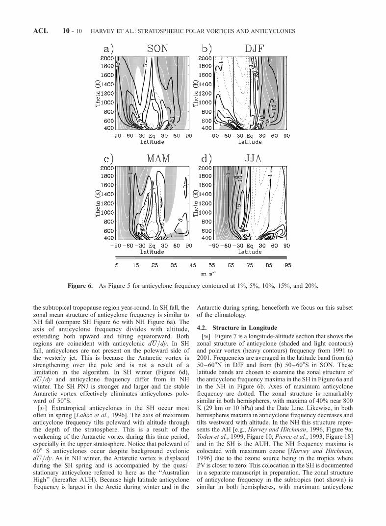
the subtropical tropopause region year-round. In SH fall, thezonal mean structure of anticyclone frequency is similar toNH fall (compare SH Figure 6c with NH Figure 6a). Theaxis of anticyclone frequency divides with altitude,extending both upward and tilting equatorward. Bothregions are coincident with anticyclonic dU=dy. In SHfall, anticyclones are not present on the poleward side ofthe westerly jet. This is because the Antarctic vortex isstrengthening over the pole and is not a result of alimitation in the algorithm. In SH winter (Figure 6d),dU=dy and anticyclone frequency differ from in NHwinter. The SH PNJ is stronger and larger and the stableAntarctic vortex effectively eliminates anticyclones pole-ward of 50�S.[35] Extratropical anticyclones in the SH occur most

often in spring [Lahoz et al., 1996]. The axis of maximumanticyclone frequency tilts poleward with altitude throughthe depth of the stratosphere. This is a result of theweakening of the Antarctic vortex during this time period,especially in the upper stratosphere. Notice that poleward of60� S anticyclones occur despite background cyclonicdU=dy. As in NH winter, the Antarctic vortex is displacedduring the SH spring and is accompanied by the quasi-stationary anticyclone referred to here as the ‘‘AustralianHigh’’ (hereafter AUH). Because high latitude anticyclonefrequency is largest in the Arctic during winter and in the

Antarctic during spring, henceforth we focus on this subsetof the climatology.

4.2. Structure in Longitude

[36] Figure 7 is a longitude-altitude section that shows thezonal structure of anticyclone (shaded and light contours)and polar vortex (heavy contours) frequency from 1991 to2001. Frequencies are averaged in the latitude band from (a)50–60�N in DJF and from (b) 50–60�S in SON. Theselatitude bands are chosen to examine the zonal structure ofthe anticyclone frequency maxima in the SH in Figure 6a andin the NH in Figure 6b. Axes of maximum anticyclonefrequency are dotted. The zonal structure is remarkablysimilar in both hemispheres, with maxima of 40% near 800K (29 km or 10 hPa) and the Date Line. Likewise, in bothhemispheres maxima in anticyclone frequency decreases andtilts westward with altitude. In the NH this structure repre-sents the AH [e.g., Harvey and Hitchman, 1996, Figure 9a;Yoden et al., 1999, Figure 10; Pierce et al., 1993, Figure 18]and in the SH is the AUH. The NH frequency maxima iscolocated with maximum ozone [Harvey and Hitchman,1996] due to the ozone source being in the tropics wherePV is closer to zero. This colocation in the SH is documentedin a separate manuscript in preparation. The zonal structureof anticyclone frequency in the subtropics (not shown) issimilar in both hemispheres, with maximum anticyclone

Figure 6. As Figure 5 for anticyclone frequency contoured at 1%, 5%, 10%, 15%, and 20%.


frequency above 1000 K near 300� longitude. However,twice as many subtropical anticyclone are identified in theNH. Sweeping poleward from low latitudes in both hemi-spheres the location of subtropical frequency maxima movesdownward and eastward, eventually merging with the west-ward tilting frequency maxima at high latitudes.

4.3. Structure in Latitude

[37] Figure 8 is a latitude-altitude section taken along thewestward-tilting dotted lines in Figure 7. The longitudes

sampled correspond to the peak in the longitudinal fre-quency distribution. Because this cross section is notaveraged over 10�, as in Figure 7, larger frequencies areobserved.[38] In SH fall (Figure 8a), an anticyclone is present over

50% of the time at 170�E, 50�S, and 600 K. The axis ofmaximum anticyclone frequency tilts poleward with altitudefrom this point to 80�S at 2000 K. In the upper stratosphere,anticyclones are near the pole during the decay of theAntarctic vortex. Similarly, in NH winter (Figure 8b), an

Figure 7. Longitude-altitude section averaged from 50� to 60� of anticyclone frequency (shaded) andpolar vortex frequency (contoured) from 1991 to 2001 in the (a) Northern Hemisphere winter and (b)Southern Hemisphere spring. Polar vortex frequency is contoured every 20%. Axes of maximumanticyclone frequency are dotted.


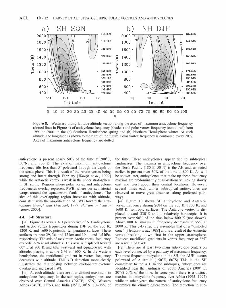
anticyclone is present nearly 50% of the time at 200�E,50�N, and 800 K. The axis of maximum anticyclonefrequency tilts less than 5� poleward through the depth ofthe stratosphere. This is a result of the Arctic vortex beingstrong and intact through February [Waugh et al., 1999]while the Antarctic vortex is weak in the upper stratospherein SH spring. Regions where polar vortex and anticyclonefrequencies overlap represent PWB, where vortex materialwraps around the equatorward flank of anticyclones. Thesize of this overlapping region increases with altitude,consistent with the amplification of PWB toward the stra-topause [Waugh and Dritschel, 1999; Polvani and Sara-vanan, 2000].

4.4. 3-D Structure

[39] Figure 9 shows a 3-D perspective of NH anticycloneand Arctic vortex frequencies during DJF on the 800 K,1200 K, and 1600 K potential temperature surfaces. Thesesurfaces are near 29, 36, and 42 km and 10, 4, and 1.5 hPa,respectively. The axis of maximum Arctic vortex frequencyexceeds 92% at all altitudes. This axis is displaced toward60� E at 800 K and tilts westward and equatorward withaltitude, placing it at the GM at 1600 K. In the westernhemisphere, the meridional gradient in vortex frequencydecreases with altitude. This 3-D depiction more clearlyillustrates the relationship between cyclone/anticycloneoverlap and increased PWB.[40] At each altitude, there are four distinct maximum in

anticyclone frequency. In the subtropics, anticyclones areobserved over Central America (290�E, 15�N), WesternAfrica (340�E, 25�N), and India (75�E, 30�N) 10–35% of

the time. These anticyclones appear tied to subtropicallandmasses. The maxima in anticyclone frequency overthe North Pacific (180�E, 50�N) is the AH and, as statedearlier, is present over 50% of the time at 800 K. As willbe shown later, anticyclones that make up these frequencymaxima are predominantly quasi-stationary, moving slowlyeast and west about their central locations. However,several times each winter subtropical anticyclones areobserved to move great distances along preferred path-ways.[41] Figure 10 shows SH anticyclone and Antarctic

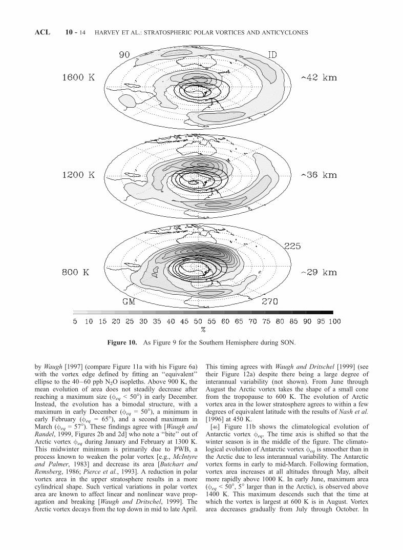
vortex frequency during SON on the 800 K, 1200 K, and1600 K isentropic surfaces. The Antarctic vortex is dis-placed toward 330�E and is relatively barotropic. It ispresent over 90% of the time below 800 K (not shown).Above 800 K, maximum frequency decreases to 55% at2000 K. This 3-D structure resembles that of a ‘‘distortedcone’’ [Mechoso et al., 1988] and is a result of the Antarcticvortex breaking down first in the upper stratosphere.Reduced meridional gradients in vortex frequency at 225�are a result of PWB.[42] There are at least two main anticyclone centers on

each level connected by a pathway of maximum frequency.The most frequent anticyclone in the SH, the AUH, occurspoleward of Australia (150�E, 60�S) This is the SHcounterpart to the AH. In the subtropics, anticyclones areidentified near the landmass of South America (300� E,20�S) 20% of the time. In some years there is a distinctmaxima in anticyclone frequency over Africa (1995–1997)while in other years the pattern of anticyclone frequencyresembles the climatological mean. The reduction in sub-

Figure 8. Westward tilting latitude-altitude section along the axes of maximum anticyclone frequency(dotted lines in Figure 4) of anticyclone frequency (shaded) and polar vortex frequency (contoured) from1991 to 2001 in the (a) Southern Hemisphere spring and (b) Northern Hemisphere winter. At eachaltitude, the longitude is shown to the right of the figure. Polar vortex frequency is contoured every 20%.Axes of maximum anticyclone frequency are dotted.


tropical anticyclone frequency compared to the NH and thepathway of maximum anticyclone frequency connecting thetwo is likely due to ‘‘repeating sequences of anticyclo-genesis, eastward advection and decay’’ [Lahoz et al.,1996].

5. Evolution of Polar Vortex and AnticycloneArea

[43] Next we examine the temporal evolution of polarvortex and anticyclone area as a function of potentialtemperature. Area is calculated in km2 and then convertedinto equivalent latitude feq [Butchart and Remsberg, 1986].feq is equal to the area enclosed by latitude circles thuslarger feq corresponds to a smaller area. Here, 10 years offeq time-altitude sections are averaged and the mean evo-lution of area is shown.

5.1. Polar Vortices

[44] Figure 11 is the climatological evolution of polarvortex feq. Below 500 K in both hemispheres, polar vortexfeq persists near 60� without a clear annual cycle. Asmentioned earlier, this is a result of biases due to theyear-round presence of the subtropical jet streams. There-fore, this discussion focuses on altitudes above 500 K.[45] The Arctic vortex (Figure 11a) forms over the course

of about a week from the top down in mid-September. Itexpands at the same rate at all altitudes until late October, atwhich time it grows more rapidly in the upper stratosphere.From October through December, the Arctic vortex istypically cone shaped, with area increasing with altitude.The evolution of Arctic vortex area below 900 K is suchthat area maximizes (feq = 63�) in late November, thenslowly decreases through April and the final warming.These results agree with calculations performed at 700 K

Figure 9. Arctic winter anticyclone (shaded) and polar vortex (contoured) frequencies from 1991 to2001 on the 800, 1200, and 1600 K isentropic surfaces. The center of each projection is the North Pole,the outer circle is the equator, latitude circles are drawn every 10�, and a polar stereographic map isdrawn. Arctic vortex frequency is contoured in 20% intervals beginning at 10%. Anticyclone frequency isshaded every 5% beginning at 5%.


by Waugh [1997] (compare Figure 11a with his Figure 6a)with the vortex edge defined by fitting an ‘‘equivalent’’ellipse to the 40–60 ppb N2O isopleths. Above 900 K, themean evolution of area does not steadily decrease afterreaching a maximum size (feq < 50�) in early December.Instead, the evolution has a bimodal structure, with amaximum in early December (feq = 50�), a minimum inearly February (feq = 65�), and a second maximum inMarch (feq = 57�). These findings agree with [Waugh andRandel, 1999, Figures 2b and 2d] who note a ‘‘bite’’ out ofArctic vortex feq during January and February at 1300 K.This midwinter minimum is primarily due to PWB, aprocess known to weaken the polar vortex [e.g., McIntyreand Palmer, 1983] and decrease its area [Butchart andRemsberg, 1986; Pierce et al., 1993]. A reduction in polarvortex area in the upper stratosphere results in a morecylindrical shape. Such vertical variations in polar vortexarea are known to affect linear and nonlinear wave prop-agation and breaking [Waugh and Dritschel, 1999]. TheArctic vortex decays from the top down in mid to late April.

This timing agrees with Waugh and Dritschel [1999] (seetheir Figure 12a) despite there being a large degree ofinterannual variability (not shown). From June throughAugust the Arctic vortex takes the shape of a small conefrom the tropopause to 600 K. The evolution of Arcticvortex area in the lower stratosphere agrees to within a fewdegrees of equivalent latitude with the results of Nash et al.[1996] at 450 K.[46] Figure 11b shows the climatological evolution of

Antarctic vortex feq. The time axis is shifted so that thewinter season is in the middle of the figure. The climato-logical evolution of Antarctic vortex feq is smoother than inthe Arctic due to less interannual variability. The Antarcticvortex forms in early to mid-March. Following formation,vortex area increases at all altitudes through May, albeitmore rapidly above 1000 K. In early June, maximum area(feq < 50�, 5� larger than in the Arctic), is observed above1400 K. This maximum descends such that the time atwhich the vortex is largest at 600 K is in August. Vortexarea decreases gradually from July through October. In

Figure 10. As Figure 9 for the Southern Hemisphere during SON.


November and December, the Antarctic vortex decays fromthe top down. Compared to the structure of the Arctic vortexin NH summer, from late December through February theAntarctic vortex is a deeper cone with a base 5 times larger.This evolution agrees with Waugh and Randel [1999](compare Figure 11b with their Figure 4b).

5.2. Anticyclones

[47] Figure 12 shows the climatological evolution ofanticyclone area in the NH as a function of altitude. Inthe NH (Figure 12a), anticyclone area increases at all levelsin late August, several weeks before the formation of theArctic vortex. This is likely the time when the summertimecircumpolar anticyclone ceases to encircle the pole. At thistime anticyclone area is constant with altitude. In earlywinter (SON), anticyclone area maximizes below 700 K and

minimizes above 1000 K such that area decreases withaltitude. The minimum in the upper stratosphere occurswhen the Arctic vortex is growing while polar vortex area issteady below 700 K (compare Figure 12a to Figure 11a). Inmid to late November, when Arctic vortex area plateaus,anticyclone area begins to increase. During December andJanuary, when the Arctic vortex temporarily shrinks, anti-cyclone area maximizes. The timing of this maximum isconsistent with the results of Harvey and Hitchman [1996]who found January to be the month of maximum AHfrequency at 10 hPa. Above 1000 K in February and March,the same altitude and time where recovery of the Arcticvortex is observed, anticyclone area decreases. During Apriland May, area is again constant with altitude and decreasesmore gradually than the rate of increase in August. Anti-cyclones are identified to some extent year-round below

Figure 11. Time-altitude sections of average polar vortex area from 1991 to 2001 in the (a) NorthernHemisphere and b) Southern Hemisphere. Area is expressed in terms of equivalent latitude (feq). Contourinterval is 5�.


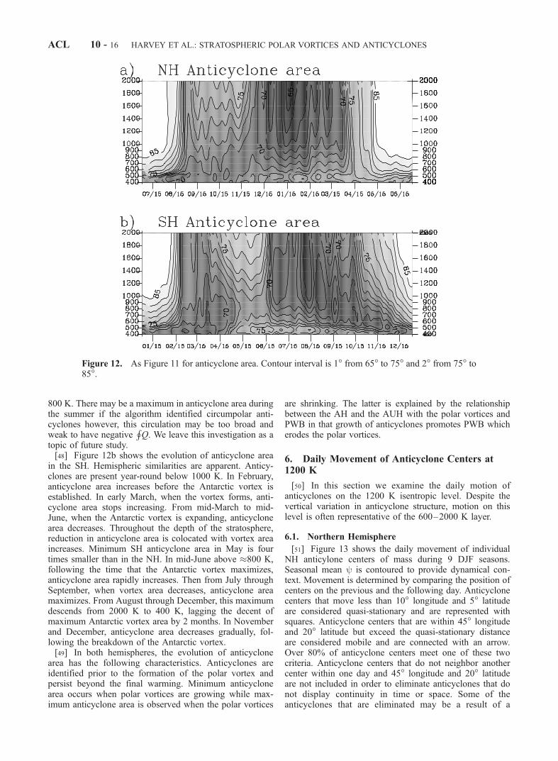
800 K. There may be a maximum in anticyclone area duringthe summer if the algorithm identified circumpolar anti-cyclones however, this circulation may be too broad andweak to have negative

HQ. We leave this investigation as a

topic of future study.[48] Figure 12b shows the evolution of anticyclone area

in the SH. Hemispheric similarities are apparent. Anticy-clones are present year-round below 1000 K. In February,anticyclone area increases before the Antarctic vortex isestablished. In early March, when the vortex forms, anti-cyclone area stops increasing. From mid-March to mid-June, when the Antarctic vortex is expanding, anticyclonearea decreases. Throughout the depth of the stratosphere,reduction in anticyclone area is colocated with vortex areaincreases. Minimum SH anticyclone area in May is fourtimes smaller than in the NH. In mid-June above �800 K,following the time that the Antarctic vortex maximizes,anticyclone area rapidly increases. Then from July throughSeptember, when vortex area decreases, anticyclone areamaximizes. From August through December, this maximumdescends from 2000 K to 400 K, lagging the decent ofmaximum Antarctic vortex area by 2 months. In Novemberand December, anticyclone area decreases gradually, fol-lowing the breakdown of the Antarctic vortex.[49] In both hemispheres, the evolution of anticyclone

area has the following characteristics. Anticyclones areidentified prior to the formation of the polar vortex andpersist beyond the final warming. Minimum anticyclonearea occurs when polar vortices are growing while max-imum anticyclone area is observed when the polar vortices

are shrinking. The latter is explained by the relationshipbetween the AH and the AUH with the polar vortices andPWB in that growth of anticyclones promotes PWB whicherodes the polar vortices.

6. Daily Movement of Anticyclone Centers at1200 K

[50] In this section we examine the daily motion ofanticyclones on the 1200 K isentropic level. Despite thevertical variation in anticyclone structure, motion on thislevel is often representative of the 600–2000 K layer.

6.1. Northern Hemisphere

[51] Figure 13 shows the daily movement of individualNH anticylone centers of mass during 9 DJF seasons.Seasonal mean y is contoured to provide dynamical con-text. Movement is determined by comparing the position ofcenters on the previous and the following day. Anticyclonecenters that move less than 10� longitude and 5� latitudeare considered quasi-stationary and are represented withsquares. Anticyclone centers that are within 45� longitudeand 20� latitude but exceed the quasi-stationary distanceare considered mobile and are connected with an arrow.Over 80% of anticyclone centers meet one of these twocriteria. Anticyclone centers that do not neighbor anothercenter within one day and 45� longitude and 20� latitudeare not included in order to eliminate anticyclones that donot display continuity in time or space. Some of theanticyclones that are eliminated may be a result of a

Figure 12. As Figure 11 for anticyclone area. Contour interval is 1� from 65� to 75� and 2� from 75� to85�.


circulation temporarily weakening such that the algorithmfails to identify it over its entire lifetime. Anticyclonecenters are colored based on elapsed days between 1December and 28 February. The duration of each color isabout a week. It is common for multiple anticyclones to bepresent on a given day. This occurs when like coloredcenters are in different places and are not connected to eachother. While difficult to detect in this figure, the merger ofanticyclones occurs when like colors approach each other.Anticyclones identified near the pole (1994/1995, 1997/1998, 1998/1999, and 2000/2001) are observed duringSSWs.[52] Anticyclones that comprise the four anticyclone

frequency maxima (see Figure 9) are often quasi-stationaryor slowly vacillate about their central locations. An impor-

tant consequence of the quasi-stationary AH is that itdisplaces the Arctic vortex toward lower latitudes thatmay be sunlit, thus activating chemically processed air,which increases ozone loss [Degorska and Rajewska-Wiech,1996]. Several times each winter an anticyclone can betracked continuously over great distances. Examples of thislong range motion include from India toward the Date Linein 2000/2001, from Africa toward the Date Line in 1992/1993, 1993/1994, 1994/1995, 1995/1996, and 1997/1998,from Central America to Africa in 1992/1993, 1993/1994,1996/1997, 1997/1998, and 1999/2000, from Central Amer-ica eastward all the way to the Date Line in 1992/1993,1997/1998, from India toward Africa in 1998/1999, andfrom Africa to Central America in 1994/1995. Less frequentpaths are observed from Central America and India to the

Figure 13. Daily position and movement of Northern Hemisphere anticyclones for each DJF seasonfrom 1992 to 2001 on the 1200 K isentropic surface. Contour interval is 10%. See color version of thisfigure at back of this issue.


Pole in 2000/2001. One can see from this list and from aquick inspection of the figure that sustained continuousmotion occurs most often from Central America to Africaand from Africa toward the Date Line. In these cases, as ananticyclone moves eastward it also moves poleward. Thispoleward motion acts to strengthen anticyclonic circulationsin the conservation of absolute vorticity. While the causes ofanticyclogenesis at low latitudes remains illusive, equator-ward displacement of the polar vortex [Waugh, 1993] andinertial instability [Knox, 1997; Rosier and Lawrence, 1999]are suspected to play a role in the propagation of distur-bances out of the tropics.

6.2. Southern Hemisphere

[53] Figure 14 shows the daily movement of individualSH anticylone centers at 1200 K during 9 SON seasons. The

same distance criteria is used to illustrate the movement ofquasi-stationary and mobile anticyclones as in the NH.Anticyclones during southern spring are either quasi-sta-tionary or, almost exclusively, move eastward. The motionof mobile anticyclones is more regular and periodic than inthe NH and they can be tracked over longer distances. Thissuggests that the lifetime of mobile anticyclones in the SHexceeds that in the NH. In particular, the subtropical anti-cyclone over South America appears to be a region ofenhanced anticyclogenesis and the beginning of a pathwayfor mobile anticyclones. In daily sequences of polar stereo-graphic projections of y (not shown), anticyclones are oftenobserved to form in the vicinity of South America and thenmigrate continuously eastward around the Antarctic vortex,past Africa and into the Australian sector. The periodicity ofthis life cycle is shorter than the life cycle itself. In other

Figure 14. As Figure 13 in the Southern Hemisphere during SON. See color version of this figure atback of this issue.


words, before an anticyclone reaches Australia another highforms over South America and begins moving eastwardalong a similar track. Hence, there are often two anti-cyclones present during the breakdown of the Antarcticvortex and the merger of anticyclones is common. Irrever-sible folding and mixing of air originating inside bothanticyclones occurs within the resulting anticyclone follow-ing a merger event [Lahoz et al., 1996]. As a mobileanticyclone moves around an elongated polar vortex, themajor axis of the polar vortex rotates in the same directionand at the same rate as the motion of the anticyclone. Thisrotation has been well documented and referred to as an‘‘eastward traveling wave 2’’ [e.g.,Mechoso and Hartmann,1982; Shiotani et al., 1990]. Once anticyclones reachAustralia their motion becomes quasi-stationary. As thearea of the Antarctic vortex decreases, anticyclones encirclehigher latitudes, eventually moving over the pole during thefinal warming. This is in contrast to the somewhat irregularbehavior of mobile anticyclones in the NH. This frequentand continuous life cycle route has transport and mixing

implications [Pierce and Fairlie, 1993]. As in the NH, theAUH displaces the Antarctic vortex from the pole and itsgrowth and decay likely influences the ozone budget.

7. Quasi-Stationary Versus TravellingAnticyclones

[54] In this section, the range of amplitude-weightedanticyclone phase speeds are computed on each potentialtemperature surface. Seasonal time periods of 90 days areused with once-daily data. On each day, level, and latitudeanticyclones are spectrally decomposed in longitude forwave numbers 1–6. On each day and for each wave numberthis results in a latitude-altitude section of spectral coef-ficients. Seasonal time series of coefficients are then con-structed at each latitude and altitude for each wave number.These time series are then spectrally decomposed in time todetermine phase speeds. Resolvable wave periods rangefrom 90 days to the Nyquist frequency of 2 days. The

Figure 15. Latitude-altitude sections of anticyclone power spectra. Rows 1–4 are each season.Columns 1–3 are stationary, eastward, and westward components. Shaded areas are where the amplitudeof wave 2 exceeds that of wave 1. Contour interval is 0.1 for the stationary waves and 0.01 for thetraveling waves.


resulting power spectrum is a function of latitude, altitude,wave period, and wave number.[55] We integrate over wave period and wave number to

identify latitudes and altitudes with power in the stationaryand traveling components. Wave periods exceeding 30 daysare considered stationary. Transient wave periods range from5 to 22.5 days. Latitude-altitude sections of power spectraare shown in Figure 15. The spectral amplitude of thestationary component is typically 10 times larger than eithertraveling component. Transient wave periods range from 6to 20 days depending on season, hemisphere, and altitude.[56] In NH fall, westward traveling wave 1 anticyclones

are observed. In NH winter, quasi-stationary wave 1 (theAH) and eastward moving waves 1 and 2 in mid to highlatitudes are accompanied by westward traveling wave 1anticyclones in the subtropics. In SH fall anticyclones movewestward in the subtropics. In SH winter there is no spectralpower at high latitudes. Instead, quasi-stationary and west-ward traveling wave 1 anticyclones and eastward travelingwave 2 anticyclones are observed in the Southern subtropics.The strength and size of the Antarctic vortex does not allowanticyclones to penetrate poleward. However, the SH springis characterized by quasi-stationary wave 1 and eastwardtraveling wave 2 in mid and high latitudes. The onlysituation where the spectral power in wave 2 exceeds thatin wave 1 is eastward moving anticyclones during NH winterand SH winter and spring. These results agree with previousstudies of the behavior of SH anticyclones [Mechoso et al.,1988, 1991; Farrara et al., 1992; Lahoz et al., 1996].

8. Summary and Conclusions

[57] In this paper we present a new algorithm which isused to identify anticyclones and polar vortices. Vortexedges are identified by integrating Q around y isopleths.Discrete regions dominated by rotation are identified from330 K to 2000 K over a 10-year period (1991–2001). Thedaily evolution of identified anticyclones is shown duringFebruary and March 1999. During this time, the algorithmsperform well during both an anticyclone merger event and amidwinter breakdown of Arctic vortex. Emphasis is placedon characterizing the structure of anticyclones and polarvortices as ‘‘objects’’ associated with distinct circulationsand enclosed air masses.[58] Seasonal mean zonal mean frequency of polar vor-

tices shows their persistence at each latitude and altitudeand their location relative to zonal mean westerly jets. TheAntarctic vortex forms more rapidly, lasts longer, and isless variable than the Arctic vortex. Anticyclones occurwhere there is background anticyclonic zonal mean windshear. In all seasons from 330 to 700 K anticyclones tiltpoleward out of the tropics and subtropics. Above 700 K,midlatitude and extratropical anticyclones are observedmost often in NH winter and SH spring. The longitudinalstructure from 50� to 60� during NH winter and SH springshow that, in both hemispheres, anticyclones and polarvortices tilt westward with altitude. Maximum anticyclonefrequency (35%) and minimum polar vortex (10%) fre-quency is observed near the Date Line. Maximum polarvortex frequency is observed near 300�E and increases withaltitude (70%). Latitude altitude cross sections along theaxes of maximum anticyclone frequency show that anti-

cyclones in the Southern spring also tilt poleward, whileNH winter anticyclones do not. Anticyclones are observed50% of the time near 50� and 700 K in NH winter and SHspring. Regions where both anticyclones and polar vorticesoccur expand with altitude due to increased PWB withheight. Analysis in 3-D revealed that, in the NH, anti-cyclones occur most often over Central America, WesternAfrica, India, and the North Pacific. In the SH anticyclonesare most often near South America, Africa, and poleward ofAustralia.[59] The evolution of both Arctic and Antarctic vortex

area agrees with results based on elliptical diagnostics[Waugh and Randel, 1999]. In both hemispheres, anticy-clones are identified prior to the formation of the polarvortex and persist beyond the final warming. In early winterin the upper stratosphere, minimum anticyclone area occurswhen polar vortex area is increasing from September toDecember in the NH and from March to June in the SH.Maximum anticyclone area occurs when the polar vorticesare shrinking. This is from December to March in the NHand from July to October in the SH. In the SH, descent ofmaximum anticyclone area lags the descent of maximum inAntarctic vortex area by 2 months. This lag is due toincreased anticyclogenesis as the vortex weakens.[60] Frequency and anticyclone motion at 1200 K is

shown for each NH winter and SH spring. In NH winter,anticyclone motion poleward of 30�N is most often east-ward while anticyclones at lower latitudes typically movetoward the west. The AH often displaces the Arctic vortexfrom the pole which is believed to be an important factorthat increases ozone loss. The AH and the anticyclone overCentral America are often quasi-stationary while motion ofthe high over Africa is less predictable. The frequency ofcross-equatorial advection of PV is colocated with maximain anticyclone frequency. This appears to be the result of thepoleward transport of air across the equator between thepolar vortex and mobile anticyclones. In SH spring, anti-cyclones form in the subtropics near South America andpropagate eastward and poleward in a periodic fashion.Before these mobile anticyclones merge with the quasi-stationary anticyclone at high latitudes near Australiaanother has formed near South America.[61] Spectral decomposition of the anticyclones is per-

formed to determine the frequency of mobile anticyclonesto stationary anticyclones. In NH fall, westward travelingwave 1 anticyclones dominate. In NH winter, quasi-sta-tionary wave 1 (the AH) and eastward moving waves 1 and2 in mid to high latitudes are accompanied by westwardtraveling wave 1 anticyclones in the subtropics. In SH fallsubtropical anticyclones travel westward. SH spring ischaracterized by quasi-stationary wave 1 and eastwardtraveling wave 2 in mid and high latitudes.[62] This climatology provides new insight into the

frequency and location of stratospheric anticyclones, thusexpanding the current knowledge of stratospheric dynamics.The formation, growth, and movement of anticyclones inthe stratosphere alter the structure of the Arctic and Ant-arctic polar vortices, the extent of springtime ozone loss,and planetary wave propagation. This work aids in under-standing these anticyclone life cycles. Future work includesintegrating chemical data into the climatology to determinethe role of traveling anticyclones in the transport of con-


stituents. Extension of the climatology into the troposphereis of interest to study trends in cyclone/anticyclone occur-rence and duration and the association between cyclones/anticyclones and the transport of smoke, dust, and pollution.

[63] Acknowledgments. The authors would like to thank AlanO’Neill and the UK Meteorological Office for producing the analyses.We would also like to thank the Distributed Active Archive Center at theGoddard Space Flight Center for distributing the data. We appreciate thereviewers’ comments and suggestions, which improved the quality of thismanuscript. M.H.H. was funded by NASA grant NAG-1-2162.

ReferencesBabiano, A., G. Boffetta, A. Provenzale, and A. Vulpiani, Chaotic advec-tion in point vortex models and two-dimensional turbulence, Phys.Fluids, 7, 2465–2474, 1994.

Bell, G. D., and L. F. Bosart, A 15-year climatology of Northern hemi-sphere 500 mb closed cyclone and anticyclone centers, Mon. WeatherRev., 117, 2142–2163, 1989.

Boville, B. W., The Aleutian stratospheric anticyclone, J. Meteorol., 17,329–336, 1960.

Brachet, M. E., M. Meneguzzi, H. Politano, and P. L. Sulem, The dynamicsof freely decaying two-dimensional turbulence, J. Fluid Mech., 194,333–349, 1988.

Butchart, N., and E. E. Remsberg, The area of the stratospheric polar vortexas a diagnostic for tracer transport on an isentropic surface, J. Atmos. Sci.,43, 1319–1339, 1986.

Chen, P., J. R. Holton, A. O’Neill, and R. Swinbank, Isentropic massexchange between the Tropics and extratropics in the stratosphere,J. Atmos. Sci., 51, 3006–3018, 1994.

Dameris, M., and V. Grewe, Three-dimensional description of the strato-spheric polar vortex, Beitr. Phys. Atmos., 67, 157–160, 1994.

Dameris, M., M. Wirth, W. Renger, and V. Grewe, Definition of the polarvortex edge by LIDAR data of the stratospheric aerosol: A comparisonwith values of potential vorticity, Beitr. Phys. Atmos., 68(2), 113–119,1995.

Degorska, M., and B. Rajewska-Wiech, The role of stratospheric minorwarmings in producing the total ozone deficiencies over Europe in1992 and 1993, J. Atmos. Terr. Phys., 58, 1855–1862, 1996.

Dewar, W. K., and G. R. Flierl, Particle trajectories and simple models oftransport in coherent vortices, in Dynamics of Atmospheres and Oceans,pp. 215–252, Elsevier Sci., New York, 1985.

Domon, K., I. Osamu, and S. Watanabe, Mass transport by a vortex ring,J. Phys. Soc. Jpn., 69, 120–123, 2000.

Elhmaidi, D., A. Provenzale, and A. Babiano, Elementary topology of twodimensional turbulence from a Lagrangian viewpoint and single particledispersion, J. Fluid Mech., 257, 533–558, 1993.

Fairlie, T. D. A., Three-dimensional transport simulations of the dispersal ofvolcanic aerosol from Mount Pinatubo, Q. J. R. Meteorol. Soc., 121,1943–1980, 1995.

Fairlie, T. D. A., and A. O’Neill, The stratospheric major warming of winter1984/85: Observations and dynamical inferences, Q. J. R. Meteorol. Soc.,114, 557–577, 1988.

Fairlie, T. D. A., A. O’Neill, and V. D. Pope, The sudden breakdown of anunusually strong cyclone in the stratosphere during winter 1988/89, Q. J.R. Meteorol. Soc., 116, 767–774, 1990.

Fairlie, T. D. A., R. B. Pierce, J. A. Al-Saadi, W. L. Grose, J. M. Russell III,M. H. Proffitt, and C. R. Webster, The contribution of mixing in Lagran-gian photochemical predictions of polar ozone loss over the Arctic insummer 1997, J. Geophys. Res., 104, 26,597–26,609, 1999.

Farrara, J. D., M. Fisher, and C. R. Mechoso, Planetary-scale disturbancesin the southern stratosphere during early winter, J. Atmos. Sci., 49, 1757–1775, 1992.

Hartmann, D., et al., Transport into the South Polar vortex in early spring,J. Geophys. Res., 94, 16,779–16,796, 1989.

Harvey, V. L., and M. H. Hitchman, A climatology of the Aleutian High,J. Atmos. Sci., 53, 2088–2101, 1996.

Haynes, P. H., High-resolution three-dimensional modelling of stratosphericflows: Quasi-two dimensional turbulence dominated by a single vortex,in Topological Fluid Mechanics, edited by H. K. Moffat and A. Tsinober,Cambridge Univ. Press, New York, 1990.

Hirota, I., K. Saotome, T. Suzuki, and S. Ikeda, Structure and behavior ofthe Aleutian anticyclone as revealed by meteorological rocket and satel-lite observations, J. Meteorol. Soc. Jpn., 51, 353–362, 1973.

Hitchman, M. H., et al., Mean winds in the tropical stratosphere and meso-sphere during January 1993, March 1994, and August 1994, J. Geophys.Res., 102, 26,033–26,052, 1997.

Hsu, C.-P., Air parcel motions during a numerically simulated sudden stra-tospheric warming, J. Atmos. Sci., 37, 2768–2792, 1980.

Jones, D. A., and I. Simmonds, A climatology of Southern hemisphereextratropical cyclones, Clim. Dyn., 9, 131–145, 1993.

Jones, D. A., and I. Simmonds, A climatology of Southern hemisphereanticyclones, Clim. Dyn., 10, 333–348, 1994.

Knox, J. A., Generalized nonlinear balance criteria and inertial stability,J. Atmos. Sci., 54, 967–985, 1997.

Koh, T.-Y., and R. A. Plumb, Lobe dynamics applied to barotropic Rossby-wave breaking, Phys. Fluids, 12, 1518–1528, 2000.

Labitzke, K., Interannual variability of the winter stratosphere in the north-ern hemisphere, Mon. Weather Rev., 105, 762–770, 1977.

Labitzke, K., Stratospheric-mesospheric midwinter disturbances: A sum-mary of observed characteristics, J. Geophys. Res., 86, 9665–9678,1981a.

Labitzke, K., The amplification of height-wave 1 in January 1979: A char-acteristic precondition for the major warming in February, Mon. WeatherRev., 109, 983–989, 1981b.

Lahoz, W. A., et al., Vortex dynamics and the evolution of water vapour inthe stratosphere of the southern hemisphere, Q. J. R. Meteorol. Soc., 122,423–450, 1996.

Lambert, S. J., A cyclone climatology of the Canadian Climate Centregeneral circulation model, J. Clim., 1, 109–115, 1988.

Malvern, L. E., Introduction to the Mechanics of a Continuous Medium,Prentice-Hall, Old Tappan, N. J., 713 pp., 1969.

Manney, G. L., and R. W. Zurek, Interhemispheric comparison of thedevelopment of the stratospheric polar vortex during fall: A 3-dimen-sional perspective for 1991–1992, Geophys. Res. Lett., 20, 1275–1278, 1993.

Manney, G. L., R. W. Zurek, M. E. Gelman, A. J. Miller, and R. Nagatani,The anomalous Arctic lower stratospheric polar vortex of 1992–1993,Geophys. Res. Lett., 21, 2405–2408, 1994.

Manney, G. L., et al., Formation of low-ozone pockets in the middle strato-spheric anticyclone during winter, J. Geophys. Res., 100, 13,939–13,950, 1995a.

Manney, G. L., et al., Lagrangian transport calculations using UARS data,part I, Passive tracers, J. Atmos. Sci., 52, 3049–3068, 1995b.

Manney, G. L., W. A. Lahoz, and R. W. Zurek, Simulation of the December1998 stratospheric major warming, Geophys. Res. Lett., 26, 2733–2736,1999.

Manney, G. L., H. A. Michelsen, F. W. Irion, G. C. Toon, M. R. Gunson,and A. E. Roche, Lamination and polar vortex development in fall fromATMOS long-lived trace gases observed during November 1994, J. Geo-phys. Res., 105, 29,023–29,038, 2000.

McIntyre, M. E., How well do we understand the dynamics of stratosphericwarmings?, J. Meteorol. Soc. Jpn., 60, 37–65, 1982.

McIntyre, M. E., and T. N. Palmer, Breaking planetary waves in the strato-sphere, Nature, 305, 593–600, 1983.

McIntyre, M. E., and T. N. Palmer, The ‘‘surf zone’’ in the stratosphere,J. Atmos. Terr. Phys., 46, 825–849, 1984.

McWilliams, J. C., The emergence of isolated coherent vortices in turbulentflow, J. Fluid Mech., 146, 21–34, 1984.

Mechoso, C. R., and D. L. Hartmann, An observational study of travelingplanetary waves in the southern hemisphere, J. Atmos. Sci., 39, 1921–1935, 1982.

Mechoso, C. R., A. O’Neill, V. D. Pope, and J. D. Farrara, A study of thestratospheric final warming of 1982 in the southern hemisphere, Q. J. R.Meteorol. Soc., 49, 1242–1263, 1988.

Mechoso, C. R., J. D. Farrara, and M. Ghil, Intraseasonal variability of thewinter circulation in the southern hemisphere atmosphere, J. Atmos. Sci.,48, 1387–1404, 1991.

Michelsen, H. A., G. L. Manney, M. R. Gunson, C. P. Rinsland, andR. Zander, Correlations of stratospheric abundances of CH4 and N2Oderived from ATMOS measurements, Geophys. Res. Lett., 25, 2777–2780, 1998.

Michelsen, H. A., et al., Intercomparison of ATMOS, SAGE II and ER-2observations in Arctic vortex and extra-vortex air masses during spring1993, Geophys. Res. Lett., 26, 291–294, 1999.

Morris, G. A., S. R. Kawa, A. R. Douglass, M. R. Schoeberl, L. Froide-vaux, and J. Waters, Low-ozone pockets explained, J. Geophys. Res.,103, 3599–3610, 1998.

Murray, R. J., and I. Simmonds, A numerical scheme for tracking cyclonecentres from digital data, part I, development and operation of thescheme, Aust. Meteorol. Mag., 39, 155–166, 1991.

Nash, E. R., P. A. Newman, J. E. Rosenfield, and M. R. Schoeberl, Anobjective determination of the polar vortex using Ertel’s potential vorti-city, J. Geophys. Res., 101, 9471–9478, 1996.

Norton, W. A., and G. D. Carver, Visualizing the evolution of the strato-spheric polar vortex in January 1992, Geophys. Res. Lett., 21, 1455–1458, 1994.


O’Neill, A., and V. D. Pope, Simulations of linear and nonlinear distur-bances in the stratosphere, Q. J. R. Meteorol. Soc., 114, 1063–1110,1988.

O’Neill, A., W. Grose, V. D. Pope, H. Maclean, and R. Swinbank, Evolu-tion of the stratosphere during Northern winter 1991/92 as diagnosedfrom U. K. Meteorological Office analyses, J. Atmos. Sci., 51, 2800–2817, 1994.

Paparella, F., A. Babiano, C. Basdevant, A. Provenzale, and P. Tanga, ALagrangian study of the Antarctic polar vortex, J. Geophys. Res., 102,6765–6773, 1997.

Pawson, S., K. Labitzke, R. Lenschow, B. Naujokat, B. Rajewski, M. Wies-ner, and R.-C. Wohlfart, Climatology of the Northern Hemisphere strato-sphere derived from Berlin analyses, part 1, Monthly means, inMeteorologische Abhandlungen, vol. 7, no. 3, Von Dietrich Reimer, Ber-lin, 1993.

Pierce, R. B., and T. D. A. Fairlie, Chaotic advection in the stratosphere:Implications for the dispersal of chemically perturbed air from the polarvortex, J. Geophys. Res., 98, 18,589–18,595, 1993.

Pierce, R. B., W. T. Blackshear, T. D. Fairlie, W. L. Grose, and R. E. Turner,The interaction of radiative and dynamical processes during a simulatedsudden stratospheric warming, J. Atmos. Sci., 50, 3829–3851, 1993.

Polvani, L. M., and R. Saravanan, The three-dimensional structure of break-ing Rossby waves in the polar wintertime stratosphere, J. Atmos. Sci., 57,3663–3685, 2000.

Polvani, L. M., D. W. Waugh, and R. A. Plumb, On the subtropical edge ofthe stratospheric surf zone, J. Atmos. Sci., 52, 1288–1309, 1995.

Price, J. D., and G. Vaughan, Statistical studies of cut-off-low systems, Ann.Geophys., 10, 96–102, 1992.

Provenzale, A., Transport by coherent barotropic vortices, Annu. Rev. FluidMech., 31, 55–93, 1999.

Randel, W. J., and F. Wu, Cooling of the Arctic and Antarctic polar strato-spheres due to ozone depletion, J. Clim., 12, 1467–1479, 1999.

Randel, W. J., et al., Stratospheric transport from the tropics to middlelatitudes by planetary-wave mixing, Nature, 365, 533–535, 1993.

Rosier, S. M., and B. N. Lawrence, The January 1992 stratospheric suddenwarming: A role for tropical inertial instability?, Q. J. R. Meteorol. Soc.,125, 2575–2596, 1999.

Rummukainen, M., B. Knudsen, and P. von der Gathen, Dynamical diag-nostics of the edges of the polar vortices, Ann. Geophys., 12, 1114–1118,1994.

Salby, M. L., D. O’Sullivan, R. R. Garcia, and P. Callaghan, Air motionsaccompanying the development of a planetary wave critical layer,J. Atmos. Sci., 47, 1179–1204, 1990.

Scherhag, R., Die explosionsartigen Stratospharenerwarmungen des Spat-winters 1952, Ber. Dtsch. Wetterdienstes (US Zone), 38, 51–63, 1952.

Schoeberl, M. R., L. R. Lait, P. A. Newman, and J. E. Rosenfield, Thestructure of the polar vortex, J. Geophys. Res., 97, 7859–7882, 1992.

Shiotani, M., K. Kuroi, and I. Hirota, Eastward traveling waves in thesouthern hemisphere stratosphere during the spring of 1983, Q. J. R.Meteorol. Soc., 116, 913–927, 1990.

Simmonds, I., and X. Wu, Cyclone behaviour response to changes in wintersouthern hemisphere sea-ice concentration, Q. J. R. Meteorol. Soc., 119,1121–1148, 1993.

Sinclair, M. R., An objective cyclone climatology for the Southern hemi-sphere, Mon. Weather Rev., 122, 2239–2256, 1994.

Sinclair, M. R., A climatology of cyclogenesis for the Southern hemisphere,Mon. Weather Rev., 123, 1602–1619, 1995.

Sinclair, M. R., A climatology of anticyclones and blocking for the South-ern hemisphere, Mon. Weather Rev., 124, 245–263, 1996.

Sinclair, M. R., Objective identification of cyclones and their circulationintensity, and climatology, Weather Forecast., 12, 595–612, 1997.

Swinbank, R., and A. O’Neill, A stratosphere-troposphere data assimilationsystem, Mon. Weather Rev., 122, 686–702, 1994.

Thorncroft, C. D., B. J. Hoskins, and M. E. McIntyre, Two paradigms ofbaroclinic-wave life-cycle behaviour, Q. J. R. Meteorol. Soc., 119, 17–55, 1993.

Trounday, B., L. Perthuis, S. Strebelle, J. D. Farrara, and C. R. Mechoso,Dispersion properties of the flow in the southern stratosphere duringwinter and spring, J. Geophys. Res., 100, 13,901–13,918, 1995.

Wang, K.-Y., and D. E. Shallcross, A Lagrangian study of the three-dimen-sional transport of boundary-layer tracers in an idealised baroclinic wavelive-cycle, J. Atmos. Chem., 35, 227–247, 2000.

Warn, T., and H. Warn, The evolution of a nonlinear critical level, Stud.Appl. Math., 59, 37–71, 1978.

Waugh, D. W., Subtropical stratospheric mixing linked to disturbances inthe polar vortices, Nature, 365, 535–537, 1993.

Waugh, D. W., Elliptical diagnostics of stratospheric polar vortices, Q. J. R.Meteorol. Soc., 123, 1725–1748, 1997.

Waugh, D. W., and D. G. Dritschel, The Dependence of Rossby WaveBreaking on the Vertical Structure of the Polar Vortex, J. Atmos. Sci.,56, 2359–2375, 1999.

Waugh, D. W., and W. J. Randel, Climatology of Arctic and Antarctic polarvortices using elliptical diagnostics, J. Atmos. Sci., 56, 1594–1613, 1999.

Waugh, D. W., et al., Fine-scale, poleward transport of tropical air duringAASE 2, Geophys. Res. Lett., 21, 2603–2606, 1994.

Waugh, D. W., W. J. Randel, S. Pawson, P. A. Newman, and E. R. Nash,Persistence of the lower stratospheric polar vortices, J. Geophys. Res.,104, 27,191–27,201, 1999.

Weiss, J. B., Transport and mixing in traveling waves, Phys. Fluids A, 5,1379–1384, 1991a.

Weiss, J. B., The dynamics of entropy transfer in two-dimensional hydro-dynamics, Physica, 273–294, 1991b.

Yang, H., Three-dimensional transport of the Ertel potential vorticity andN2O in the GFDL SKYHI Model, J. Atmos. Sci., 52, 1513–1528, 1995.

Yoden, S., T. Yamaga, S. Pawson, and U. Langematz, A composite analysisof the stratospheric sudden warmings simulated in a perpetual Januaryintegration of the Berlin TSM GCM, J. Meteorol. Soc. Jpn., 77, 431–445, 1999.

Zhou, S., M. E. Gelman, and A. J. Miller, An inter-hemisphere comparisonof the persistent stratospheric polar vortex, Geophys. Res. Lett., 27,1123–1126, 2000.

��T. D. Fairlie and R. B. Pierce, NASA Langley Research Center,

Hampton, VA, USA.V. L. Harvey, Science Applications International Corporation, MS 401B,

Hampton, VA 23681, USA. ([email protected])M. H. Hitchman, Department of Atmospheric and Oceanic Sciences,

University of Wisconsin - Madison, Madison, WI, USA.


Figure 13. Daily position and movement of Northern Hemisphere anticyclones for each DJF seasonfrom 1992 to 2001 on the 1200 K isentropic surface. Contour interval is 10%.

HARVEY ET AL.: STRATOSPHERIC POLAR VORTICES AND ANTICYCLONES

ACL 10 - 17

Figure 14. As Figure 13 in the Southern Hemisphere during SON.

HARVEY ET AL.: STRATOSPHERIC POLAR VORTICES AND ANTICYCLONES

ACL 10 - 18

a climatology of stratospheric polar vortices and anticyclonesmag/polarvortices.pdf · a...

Documents