A Classical Monetary Model

Jordi Galí

October 2015

Assumptions

� Perfect competition in goods and labor markets� Flexible prices and wages� No capital accumulation� No �scal sector� Closed economy

Outline

� The problem of households and �rms� Equilibrium: money neutrality and the determination of nominal variables� A model with money in the utility function� Optimal policy

Households

Representative household solves

maxE0

1Xt=0

�tU (Ct; Nt) (1)

subject toPtCt +QtBt � Bt�1 +WtNt +Dt (2)

for t = 0; 1; 2; :::and the solvency constraint

limT!1

Et f�t;T (BT=PT )g � 0 (3)

where �t;T � �T�tUc;T=Uc;t is the stochastic discount factor.

Optimality conditions

�Un;tUc;t

=Wt

Pt(4)

Qt = � Et

�Uc;t+1Uc;t

PtPt+1

�(5)

Speci�cation of utility:

U(Ct; Nt) =

(C1��t �11�� � N 1+'

t

1+' for � 6= 1logCt � N 1+'

t

1+' for � = 1

implied optimality conditions:Wt

Pt= C�

t N't (6)

Qt = �Et

(�Ct+1Ct

���PtPt+1

)(7)

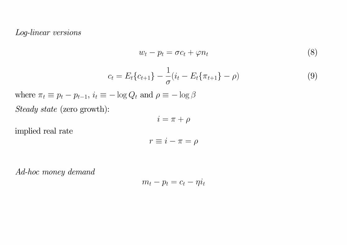
Log-linear versions

wt � pt = �ct + 'nt (8)

ct = Etfct+1g �1

�(it � Etf�t+1g � �) (9)

where �t � pt � pt�1, it � � logQt and � � � log �Steady state (zero growth):

i = � + �

implied real rater � i� � = �

Ad-hoc money demandmt � pt = ct � �it

Firms

Representative �rm with technology

Yt = AtN1��t (10)

where at � logAt follows an exogenous process

at = �aat�1 + "at

Pro�t maximization:max PtYt �WtNt

subject to (10), taking the price and wage as given (perfect competition)

Optimality condition:Wt

Pt= (1� �)AtN

��t

In log-linear termswt � pt = at � �nt + log(1� �)

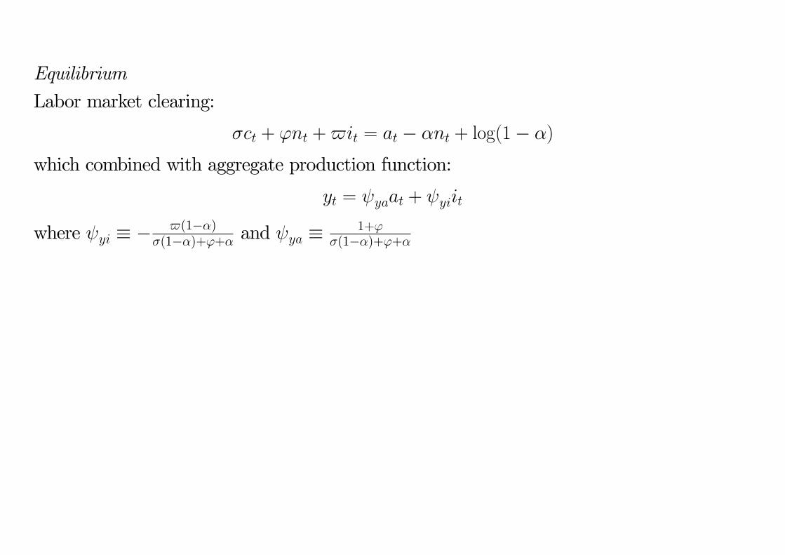
Equilibrium

Goods market clearingyt = ct

Labor market clearing�ct + 'nt = at � �nt + log(1� �)

Asset market clearing:Bt = 0

rt � it � Etf�t+1g= � + �Etf�ct+1g

Aggregate output:yt = at + (1� �)nt

Implied equilibrium values for real variables:

nt = naat + n

yt = yaat + yrt = �� � ya(1� �a)at

!t � wt � pt= at � �nt + log(1� �)

= !aat + !

where na � 1���(1��)+'+� ; n �

log(1��)�(1��)+'+� ; ya �

1+'�(1��)+'+� ;

y � (1� �) n ; !a � �+'�(1��)+'+� ; ! �

(�(1��)+') log(1��)�(1��)+'+�

=) neutrality: real variables determined independently of monetary policy=) optimal policy: undetermined.=) speci�cation of monetary policy needed to determine nominal variables

Monetary Policy and Price Level Determination

Example I: An Exogenous Path for the Nominal Interest Rate

it = i + vt

wherevt = �vvt�1 + "

vt

Implied steady state in�ation: � = i� �

Particular case: it = i for all t.Using de�nition of real rate:

Etf�t+1g = it � rt= � + vt � brt

Equilibrium in�ation: b�t = vt�1 � brt�1 + �tfor any f�tg sequence with Etf�t+1g = 0 for all t.

) nominal indeterminacy

Example II: A Simple Interest Rate Rule

it = � + � + ��(�t � �) + vt

where �� � 0. Combined with de�nition of real rate:��b�t = Etfb�t+1g + brt � vt

If �� > 1,

b�t = 1Xk=0

��(k+1)� Etfbrt+k � vt+kg

= ��(1� �a) ya�� � �a

at �1

�� � �vvt

If �� < 1, b�t = ��b�t�1 � brt�1 + vt�1 + �tfor any f�tg sequence with Etf�t+1g = 0 for all t=) nominal indeterminacy=) illustration of the "Taylor principle" requirement

Responses to a monetary policy shock (�� > 1 case):

@�t@"vt

= � 1

�� � �v< 0

@it@"vt

= � �v�� � �v

< 0

@mt

@"vt=��v � 1�� � �v

7 0

@yt@"vt

= 0

Discussion: liquidity e¤ect and price response.

Example III: An Exogenous Path for the Money Supply fmtgCombining money demand and the de�nition of the real rate:

pt =

��

1 + �

�Etfpt+1g +

�1

1 + �

�mt + ut

where ut � (1 + �)�1(�rt � yt). Solving forward:

pt =1

1 + �

1Xk=0

��

1 + �

�kEt fmt+kg + ut

where ut �P1

k=0

��1+�

�kEtfut+kg

) price level determinacy

In terms of money growth rates:

pt = mt +

1Xk=1

��

1 + �

�kEt f�mt+kg + ut

Nominal interest rate:

it = ��1 (yt � (mt � pt))

= ��11Xk=1

��

1 + �

�kEt f�mt+kg + ut

where ut � ��1(ut + yt) is independent of monetary policy.

Example�mt = �m�mt�1 + "

mt

Assume no real shocks (rt = yt = 0).

Price response:pt = mt +

��m1 + �(1� �m)

�mt

) large price response

Nominal interest rate response:

it =�m

1 + �(1� �m)�mt

) no liquidity e¤ect

A Model with Money in the Utility Function

Preferences

E0

1Xt=0

�tU

�Ct;

Mt

Pt; Nt

�Budget constraint

PtCt +QtBt +Mt � Bt�1 +Mt�1 +WtNt +Dt

with solvency constraint:limT!1

Et f�t;T (AT=PT )g � 0where At � Bt +Mt.Equivalently:

PtCt +QtAt + (1�Qt)Mt � At�1 +WtNt +Dt

Interpretation: 1�Qt = 1� expf�itg ' it

) opportunity cost of holding money

Optimality Conditions

�Un;tUc;t

=Wt

Pt

Qt = �Et

�Uc;t+1Uc;t

PtPt+1

�Um;tUc;t

= 1� expf�itg

Two cases:

� utility separable in real balances) neutrality

� utility non-separable in real balances) non-neutrality

Utility speci�cation:

U (Xt; Nt) =X1��t � 11� �

� N 1+'t

1 + 'where

Xt �"(1� #)C1��t + #

�Mt

Pt

�1��# 11�v

for � 6= 1

� C1�#t

�Mt

Pt

�#for � = 1

Note thatUc;t = (1� #)X���

t C��t

Um;t = #X���t (Mt=Pt)

��

Un;t = �N't

Implied optimality conditions:Wt

Pt= N'

t X���t C�

t (1� #)�1

Qt = �Et

(�Ct+1Ct

��� �Xt+1

Xt

�����PtPt+1

�)Mt

Pt= Ct (1� expf�itg)�

1�

�#

1� #

�1�

Log-linearized money demand equation:

mt � pt = ct � �it

where � � 1=[�(expfig � 1)] .

Log-linearized labor supply equation:

wt � pt = �ct + 'nt + (� � �)(ct � xt)

= �ct + 'nt + �(� � �) (ct � (mt � pt))

= �ct + 'nt + ��(� � �)it

where � � #1� (1��)1�1�

(1�#)1�+#1� (1��)1�1�= km(1��)

1+km(1��) 2 [0; 1) with km �M=PC =

�#

(1��)(1�#)

�1�

:

Equivalently,wt � pt = �ct + 'nt +$it

where $ � km�(1��� )

1+km(1��)

Discussion

Equilibrium

Labor market clearing:

�ct + 'nt +$it = at � �nt + log(1� �)

which combined with aggregate production function:

yt = yaat + yiit

where yi � �$(1��)

�(1��)+'+� and ya �1+'

�(1��)+'+�

Assessment of size of non-neutralities

Calibration: � = 0:99 ; � = 1 ; ' = 5 ; � = 1=4 ; � = 1=�i "large"

) $ ' km�

1 + km(1� �)> 0 ; yi ' �

km8< 0

Monetary base inverse velocity: km ' 0:3 ) yi ' �0:04M2 inverse velocity: km ' 3 ) yi ' �0:4) small output e¤ects of monetary policy

Response to monetary policy shocks (at = 0)

yt = �(mt � pt)

it = �(1=�)(1� �)(mt � pt)

where � � $(1��)�[�(1��)+'+�]+$(1��) 2 [0; 1) (assuming $ � 0)

yt = Etfyt+1g �1

�(it � Etf�t+1g �$Etf�it+1g � �)

pt = mt +�

� +$�

1Xk=1

�� +$�

1� � + � +$�

�kEtf�mt+kg

where � � �(�+')�[�(1��)+'+�]+$(1��) 2 [0; 1).

Prediction (independent of rule):

persistent money growth) cov(�m; i) > 0 and cov(�m; y) < 0

Optimal Monetary Policy with Money in the Utility Function

Social Planner�s problem

maxU

�Ct;

Mt

Pt; Nt

�subject to

Ct = AtN1��t

Optimality conditions:

�Un;tUc;t

= (1� �)AtN��t

Um;t = 0

Optimal policy (Friedman rule): it = 0 for all t .

Intuition

Implied average in�ation: � = �� < 0

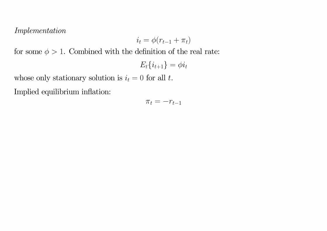
Implementationit = �(rt�1 + �t)

for some � > 1. Combined with the de�nition of the real rate:

Etfit+1g = �it

whose only stationary solution is it = 0 for all t.

Implied equilibrium in�ation:�t = �rt�1