NASA Technical Paper 3494

A Class of Stabilizing Controllers for FlexibleMultibody Systems

Suresh M. Joshi, Atul G. Kelkar, and Peiman G. Maghami

May 1995

NASA Technical Paper 3494

A Class of Stabilizing Controllers for FlexibleMultibody SystemsSuresh M. Joshi, Atul G. Kelkar, and Peiman G. MaghamiLangley Research Center � Hampton, Virginia

National Aeronautics and Space AdministrationLangley Research Center � Hampton, Virginia 23681-0001

May 1995

Abstract

This paper considers the problem of controlling a class of

nonlinear multibody exible space systems consisting of a exible

central body to which a number of articulated appendages are

attached. Collocated actuators and sensors are assumed, and

global asymptotic stability of such systems is established under

a nonlinear dissipative control law. The stability is shown tobe robust to unmodeled dynamics and parametric uncertainties.

For a special case in which the attitude motion of the central

body is small, the system, although still nonlinear, is shown to

be stabilized by linear dissipative control laws. Two types of linear

controllers are considered: static dissipative (constant gain) and

dynamic dissipative. The static dissipative control law is also

shown to provide robust stability in the presence of certain classes

of actuator and sensor nonlinearities and actuator dynamics. The

results obtained for this special case can also be readily applied for

controlling single-body linear exible space structures. For this

case, a synthesis technique for the design of a suboptimal dynamic

dissipative controller is also presented. The results obtained in

this paper are applicable to a broad class of multibody and single-

body systems such as exible multilink manipulators, multipayload

space platforms, and space antennas. The stability proofs use

the Lyapunov approach and exploit the inherent passivity of such

systems.

1. Introduction

A class of spacecraft envisioned for the future will require exible multibody systems suchas space platforms with multiple articulated payloads and space-based manipulators used for

satellite assembly and servicing. Examples of such systems include the Earth Observing System

(EOS) and Upper Atmospheric Research Satellite (UARS). (See refs. 1 and 2, respectively.)

These systems are expected to have signi�cant exibility in their structural members as well as

joints. Control system design for such systems is a di�cult problem because of the highly

nonlinear dynamics, large number of signi�cant elastic modes with low inherent damping,

and uncertainties in the mathematical model. The published literature contains a number of

important stability results for some subclasses of this problem (e.g., linear exible structures,

nonlinear multibody rigid structures, and most recently, multibody exible structures). Under

certain conditions, the input-output maps for such systems can be shown to be passive. (See

ref. 3.) The Lyapunov and passivity approaches are used in reference 4 to demonstrate global

asymptotic stability (g.a.s.) of linear exible space structures (with no articulated appendages)

for a class of dissipative compensators. The stability properties were shown to be robust to �rst-

order actuator dynamics and certain actuator-sensor nonlinearities. Multibody rigid structures

represent another class of systems for which stability results have been advanced. Subject

to a few restrictions, these systems can be ideally categorized as natural systems. (See ref. 5.)

Such systems are known to exhibit global asymptotic stability under proportional-and-derivative

(PD) control. After recognition that rigid manipulators belong to the class of natural systems,

a number of researchers (refs. 6{9) established global asymptotic stability of terrestrial rigid

manipulators by using PD control with gravity compensation. Stability of tracking controllers

was investigated in references 10 and 11 for rigid manipulators. In reference 12, the results

of reference 11 were extended to accomplish exponentially stable tracking control of exible

multilink manipulators local to the desired trajectory. Lyapunov stability of multilink exiblesystems was addressed in reference 13. However, the global asymptotic stability of nonlinear,multilink, exible space structures, which to date has not been addressed in the literature, isthe principal subject of this paper.

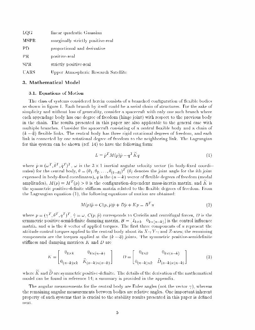
The structure to be considered is a complete nonlinear rotational dynamic model of amultibody exible spacecraft which is assumed to have a branched geometry, (i.e., a central exible body with various exible appendage bodies). (See �g. 1.) Throughout this paper,actuators and sensors are assumed to be collocated. Global asymptotic stability of such systemscontrolled by a nonlinear dissipative controller is proved. In many applications, the centralbody has large mass and moments of inertia when compared with that of the appendage bodies.As a result, the motion of the central body is small and can be considered to be in the linearrange. For this case, robust stability is proved with linear static as well as with linear dynamicdissipative compensators. The e�ects of realistic nonlinearities in the actuators and sensors arealso investigated. The stability proofs use Lyapunov's method (ref. 9) and LaSalle's theorem. Forsystems with linear collocated actuators and sensors, the stability proof by Lyapunov's methodcan take a simpler form if the work-energy rate principle (ref. 13) is used. However, because thework-energy rate principle is applicable only when the system is holonomic and scleronomic innature, a more direct approach is used here in evaluating the time derivative of the Lyapunovfunction which makes the results more general.

The organization of the paper is as follows. In section 3, a nonlinear mathematical model ofa generic exible multibody system is given. A special property of the system, which is pivotalto the proofs, and some basic kinematic relations of the quaternion (i.e., measure of attitude ofthe central body) are given. Section 4 establishes the global asymptotic stability of the completenonlinear system under a nonlinear control law based on quaternion feedback. A special case, inwhich the central body attitude motion is small, is considered in section 5. Global asymptoticstability is proved under static dissipative compensation, and these results are extended tothe case in which certain actuator and sensor nonlinearities are present. In addition, dynamicdissipative compensators, a more versatile class of dissipative compensators, are considered.Section 6 presents the application of the results to the important special case of linear single-body spacecraft. Two numerical examples are given in section 7 and some concluding remarksare given in section 8.

2. Symbols

A system matrix

eA diagonal matrix (eq. (79))

B control in uence matrix

eB diagonal matrix (eq. (80))

C Coriolis and centrifugal force coe�cient matrix

eC diagonal matrix of squares of eigenvalues

D damping matrix

eD structural damping matrix

E Euler transformation matrix; modulus of elasticity

F compensator output matrix

G(s); G0(s) plant transfer function

2

GAi(s) actuator transfer function

Ga acceleration gain matrix

Gp;Gp position gain matrices

Gr rate gain matrix

H estimator gain matrix

Ik k � k identity matrix

i index variable

J inertia matrix of single-body spacecraft

J performance index

j index variable

K sti�ness matrix of system

bK sti�ness matrix of system for linear case

eK sti�ness matrix for exible degrees of freedom

K(s) controller transfer function

k number of rigid body degrees of freedom

L Lagrangian of system

Lk2e extended Lebesgue space

M(p) mass-inertia matrix of system

cM mass-inertia matrix of system for linear case

n number of total degrees of freedom

nq number of exible degrees of freedom

P Lyapunov matrix

p;bp generalized coordinate vectors

ep vector of rigid body coordinates

Qp; Qr output weighting matrices

q vector of exural coordinates

R control weighting matrix

S skew-symmetric matrix

S property of the system

s Laplace variable

T terminal time; kinetic energy

T (s) transfer matrix

u vector of control input

V Lyapunov function candidate

v integrator output

3

x;x state vectors

ya acceleration output

yp position output

yr rate output

z state vector

� the quaternion

b�i ith component of unit vector along eigenaxis

� vector part of quaternion

�i ith component of quaternion

� scalar de�ned as (�4� 1)

integral of !

� transformation matrix

� performance function

� state vector

� Euler angle vector

� vector of rotational degrees of freedom between rigid bodies

� diagonal matrix (eq. (82))

� scalar gain

� input to nonlinearity

� state vector

�i damping in ith structural mode

& controller state vector

� mode shape matrix

� Euler rotation

' de�ned as ��

ai actuator nonlinearity (ith loop)

pi position sensor nonlinearity (ith loop)

ri rate sensor nonlinearity (ith loop)

cross product operator of vector !

! angular velocity vector for central body

Abbreviations:

a.s. asymptotically stable

DDC dynamic dissipative controller

EOS Earth Observing System

g.a.s. globally asymptotically stable

4

LQG linear quadratic Gaussian

MSPR marginally strictly positive-real

PD proportional and derivative

PR positive-real

SPR strictly positive-real

UARS Upper Atmospheric Research Satellite

3. Mathematical Model

3.1. Equations of Motion

The class of systems considered herein consists of a branched con�guration of exible bodiesas shown in �gure 1. Each branch by itself could be a serial chain of structures. For the sake ofsimplicity and without loss of generality, consider a spacecraft with only one such branch whereeach appendage body has one degree of freedom (hinge joint) with respect to the previous bodyin the chain. The results presented in this paper are also applicable to the general case withmultiple branches. Consider the spacecraft consisting of a central exible body and a chain of(k � 3) exible links. The central body has three rigid rotational degrees of freedom, and eachlink is connected by one rotational degree of freedom to the neighboring link. The Lagrangianfor this system can be shown (ref. 14) to have the following form:

L = _pTM(p) _p� qT eKq (1)

where _p = (!T; _�T ; _qT)T , ! is the 3� 1 inertial angular velocity vector (in body-�xed coordi-nates) for the central body, � = (�1; �2; : : : ; �(k�3))

T (�i denotes the joint angle for the ith joint

expressed in body-�xed coordinates), q is the (n� k) vector of exible degrees of freedom (modal

amplitudes), M(p) =MT(p) > 0 is the con�guration-dependent mass-inertia matrix, and eK isthe symmetric positive-de�nite sti�ness matrix related to the exible degrees of freedom. Fromthe Lagrangian equation (1), the following equations of motion are obtained:

M(p)�p+ C(p; _p)_p+D _p+Kp = BTu (2)

where p = ( T; �T ; qT)T , _ = !, C(p; _p) corresponds to Coriolis and centrifugal forces, D is thesymmetric positive-semide�nite damping matrix, B = [ Ik�k 0k�(n�k) ] is the control in uencematrix, and u is the k vector of applied torques. The �rst three components of u represent theattitude control torques applied to the central body about its X-, Y -, and Z-axes; the remainingcomponents are the torques applied at the (k� 3) joints. The symmetric positive-semide�nitesti�ness and damping matrices K and D are

K =

"0k�k 0k�(n�k)

0(n�k)�keK(n�k)�(n�k)

#D =

"0k�k 0k�(n�k)

0(n�k)�keD(n�k)�(n�k)

#(3)

where eK and eD are symmetric positive-de�nite. The details of the derivation of the mathematicalmodel can be found in reference 14; a summary is provided in the appendix.

The angular measurements for the central body are Euler angles (not the vector ), whereasthe remaining angular measurements between bodies are relative angles. One important inherentproperty of such systems that is crucial to the stability results presented in this paper is de�nednext.

5

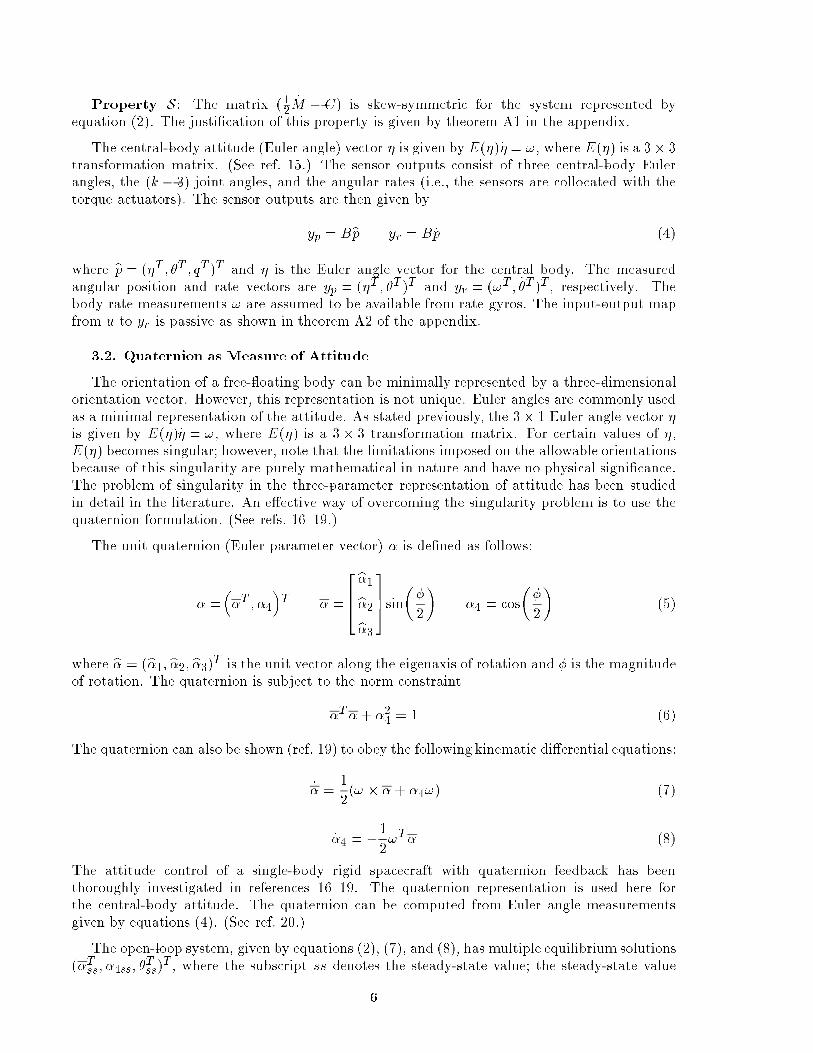
Property S: The matrix (12_M � C) is skew-symmetric for the system represented by

equation (2). The justi�cation of this property is given by theorem A1 in the appendix.

The central-body attitude (Euler angle) vector � is given by E(�)_� = !, where E(�) is a 3� 3transformation matrix. (See ref. 15.) The sensor outputs consist of three central-body Eulerangles, the (k � 3) joint angles, and the angular rates (i.e., the sensors are collocated with thetorque actuators). The sensor outputs are then given by

yp = Bbp yr = B _p (4)

where bp = (�T ; �T ; qT)T and � is the Euler angle vector for the central body. The measuredangular position and rate vectors are yp = (�T; �T)T and yr = (!T ; _�T)T, respectively. Thebody rate measurements ! are assumed to be available from rate gyros. The input-output mapfrom u to yr is passive as shown in theorem A2 of the appendix.

3.2. Quaternion as Measure of Attitude

The orientation of a free- oating body can be minimally represented by a three-dimensionalorientation vector. However, this representation is not unique. Euler angles are commonly usedas a minimal representation of the attitude. As stated previously, the 3� 1 Euler angle vector �is given by E(�)_� = !, where E(�) is a 3� 3 transformation matrix. For certain values of �,E(�) becomes singular; however, note that the limitations imposed on the allowable orientationsbecause of this singularity are purely mathematical in nature and have no physical signi�cance.The problem of singularity in the three-parameter representation of attitude has been studiedin detail in the literature. An e�ective way of overcoming the singularity problem is to use thequaternion formulation. (See refs. 16{19.)

The unit quaternion (Euler parameter vector) � is de�ned as follows:

� =��T ; �4

�T � =

264b�1b�2b�3

375sin��

2

��4 = cos

��

2

�(5)

where b� = (b�1; b�2; b�3)T is the unit vector along the eigenaxis of rotation and � is the magnitudeof rotation. The quaternion is subject to the norm constraint

�T�+ �24= 1 (6)

The quaternion can also be shown (ref. 19) to obey the following kinematic di�erential equations:

_� =1

2(! � �+ �4!) (7)

_�4 = �1

2!T� (8)

The attitude control of a single-body rigid spacecraft with quaternion feedback has beenthoroughly investigated in references 16{19. The quaternion representation is used here forthe central-body attitude. The quaternion can be computed from Euler angle measurementsgiven by equations (4). (See ref. 20.)

The open-loop system, given by equations (2), (7), and (8), has multiple equilibrium solutions(�Tss; �4ss; �

Tss)

T, where the subscript ss denotes the steady-state value; the steady-state value

6

of q is zero. By de�ning � = (�4� 1) and denoting _p = z, equations (2), (7), and (8) can berewritten as

M _z + Cz +Dz + ~Kq = BTu (9a)"_�

_q

#=�0(n�3)�3 I(n�3)�(n�3)

�z (9b)

_� =1

2[! � �+(� + 1)!] (10)

_� = �1

2!T� (11)

In equation (9a) the matrices M and C are functions of p and (p; _p), respectively. Note that the

�rst three elements of p associated with the orientation of the central body can be fully described

by the unit quaternion. Hence, M and C are implicit functions of �, and therefore the system

represented by equations (9){(11) is time-invariant and can be expressed in the state-space form

as follows:

_x = f(x; u) (12)

where x = (�T ; �; �T ; qT; zT)T . Note that the dimension of x is (2n+ 1), which is one more

than the dimension of the system in equation (2). However, the constraint of equation (6) is

now present. Veri�cation that the constraint of equation (6) is satis�ed for all t > 0 if it is

satis�ed at t = 0 easily follows from equations (7) and (8).

4. Nonlinear Dissipative Control Law

Consider the dissipative control law u, given by

u = �Gpep�Gryr (13)

where ep = (�T ; �T)T . Matrices Gp and Gr are symmetric positive-de�nite k � k matrices; Gp is

given by

Gp =

24�1 +

(�+1)2

�Gp1 03�(k�3)

0(k�3)�3 Gp2(k�3)�(k�3)

35 (14)

Note that equations (13) and (14) represent a nonlinear control law. If Gp and Gr satisfy certain

conditions, this control law can be shown to render the time rate of change of the system's energy

negative along all trajectories (i.e., it is a dissipative control law).

The closed-loop equilibrium solution can be obtained by equating all the derivatives to zero

in equations (2), (10), and (11). In particular, _p = �p = 0) ! = 0; _� = 0; _q = 0, and

�BTGpep ="�Gpep

0(n�k)�1

#=

"0k�1eKq

#(15)

Because of equation (6), j� + 1j � 1. Therefore Gp is positive-de�nite and equation (15) impliesep = (�T ; �T)T = 0 and q = 0. The equilibrium solution of equation (11) is � = �ss= Constant

(i.e., �4 = Constant), which implies from equation (6) that �4 = �1. Thus, there appear to

be two closed-loop equilibrium points corresponding to �4 = 1 and �4 = �1 (all other state

variables are zero). However, from equations (5), �4 = 1) � = 0, and �4 = �1) � = 2� (i.e.,

only one equilibrium point exists in the physical space).

One of the objectives of the control law is to transfer the state of the system from one orien-

tation (i.e., equilibrium position) to another orientation. Without loss of generality, the target

7

orientation can be de�ned to be zero, and the initial orientation, given by (�(0); �4(0); �(0)),can always be de�ned in such a way that j�i(0)j � �, 0 � �4(0) � 1 (corresponds to j�j � �),and (�(0); �4(0)) satisfy equation (6).

The following theorem establishes the global asymptotic stability of the physical equilibriumstate of the system.

Theorem 1: Suppose Gp2(k�3)�(k�3)and Grk�k

are symmetric and positive-de�nite, and

Gp1 = �I3, where � > 0. Then, the closed-loop system given by equations (12) and (13) isglobally asymptotically stable (g.a.s.).

Proof: Consider the candidate Lyapunov function

V =1

2_pTM(p) _p+

1

2qT eKq +

1

2�TGp2� +

1

2�T

�Gp1+ 2�I3

�� + ��2 (16)

Here, V is clearly positive-de�nite and radially unbounded with respect to a state vector(�T ; �; �T; qT; _pT)T because M(p), eK, Gp1, and Gp2 are all positive-de�nite symmetric matrices.Note that the matrixM(p), although con�guration dependent, is uniformly bounded from belowand above by the values which correspond to the minimum and maximum inertia con�gurations,respectively (i.e., there exist positive-de�nite matrices M and M such that M �M �M). Thetime derivative of V results in

_V = _pTM�p+1

2_pT _M _p+ _qT eKq + _�TGp2� + _�

T�Gp1+ 2�I3

��+ 2� _�� (17)

With the use of equations (2), (4), (10), (11), and (14),

_V = _pTBTu+ _pT�1

2_M � C

�_p� _pTD _p� _pTKp+ _qT eKq + _�TGp2�

+1

2(�)TGp1� +

1

2(� + 1)!TGp1�+ �!T� (18)

where = (!�) denotes the skew-symmetric cross product matrix (i.e., ! � x = x). With the

substitution for u, the fact that _pTKp = _qT eKq and (�)TGp1� = 0, and the use of property Sof the system, equation (18) becomes

_V = � _pT�D + BTGrB

�_p�(B _p)TGpep+ 1

2(� + 1)!TGp1�+ �!T�+ _�TGp2� (19)

Note that (B _p)TGpep = 1

2(� + 1)!TGp1� + �!T� + _�TGp2�. After several cancellations,

_V = � _pT�D +BTGrB

�_p (20)

Because (D +BTGrB) is a positive-de�nite symmetric matrix, _V � 0 (i.e., _V is negative-semide�nite) and _V = 0) _p = 0) �p = 0. By substitution in the closed-loop equation, equa-tion (15) results. As shown previously, equation (15) ) ep = 0 and q = 0; i.e., � = 0, � = 0, and�4 = �1 (or � = 0 or �2). Consistent with the previous discussion, these values correspond totwo equilibrium points representing the same physical equilibrium state.

From equation (16), veri�cation easily follows that any small perturbation � in �4 from theequilibrium point corresponding to �4 = �1 will cause a decrease in the value of V (� > 0 becausej�4j � 1). Thus, in the mathematical sense, �4 = �1 corresponds to an isolated equilibrium

8

point such that _V = 0 at that point and _V < 0 in the neighborhood of that point (i.e., �4 = �1is a repeller and not an attractor). Previously, _V has been shown to be negative along alltrajectories in the state space except at the two equilibrium points. That is, if the system'sinitial condition lies anywhere in the state space except at the equilibrium point correspondingto �4 = �1, then the system will asymptotically approach the origin (i.e., x = 0); if the systemis at the equilibrium point corresponding to �4 = �1 at t = 0, then it will stay there for all t > 0.However, this is the same equilibrium point in the physical space; hence, by LaSalle's invariancetheorem, the system is globally asymptotically stable. Q.E.D.

5. Systems in Attitude-Hold Con�guration

Consider a special case where the central-body attitude motion is small. This can occur inmany real situations. For example, in cases of space station-based or shuttle-based manipulators,the inertia of the base (central body) is much greater than that of any manipulator linkor payload. In such cases, the rotational motion of the base can be assumed to be in thelinear region, although the payloads (or links) attached to it can undergo large rotationaland translational motions and nonlinear dynamic loading because of Coriolis and centripetalaccelerations. The attitude of the central body is simply (the integral of the inertial angularvelocity !) and the use of quaternions is not necessary. The equations of motion (2) can now beexpressed in the state-space form simply as

_x =

"0 I

�M�1K �M�1(C +D)

#x+

"0

BT

#u (21)

where x = (pT ; _pT)T , p = ( T; �T ; qT)T , and M and C are functions of x.

5.1. Stability With Static Dissipative Controllers

The static dissipative control law u is given by

u = �Gpyp �Gryr (22)

where Gp is symmetric positive-de�nite k � k matrix and

yp = Bp yr = B _p (23)

where yp and yr are measured angular position and rate vectors, respectively.

Theorem 2: Suppose Gpk�kand Grk�k

are symmetric and positive-de�nite. Then, theclosed-loop system given by equations (21){(23) is globally asymptotically stable.

Proof: Consider the candidate Lyapunov function

V =1

2_pTM(p) _p+

1

2pT�K +BTGpB

�p (24)

Clearly, V is positive-de�nite because M(p) and (K + BTGpB) are positive-de�nite symmetric

matrices. De�ning K = (K + BTGpB), the time derivative of V can be shown to be

_V = _pT�1

2_M � C

�_p� _pTKp+ _pTKp� _pT

�D +BTGrB

�_p (25)

Again, with the use of property S, _pT(12_M � C) _p = 0, and after some cancellations,

_V = � _pT�D +BTGrB

�_p (26)

9

Because (D +BTGrB) is a positive-de�nite matrix, _V � 0 (i.e., _V is negative-semide�nite in pand _p and _V = 0) _p = 0) �p = 0). With substitution in the closed-loop equation (2) and u

given by equation (22), �K + BTGpB

�p = 0 ) p = 0 (27)

Thus, _V is not zero along any trajectories; then, by LaSalle's theorem, the system is g.a.s. Q.E.D.

The signi�cance of the two results presented in theorems 1 and 2 is that any nonlinearmultibody system belonging to these classes can be robustly stabilized with the dissipativecontrol laws given. In the case of manipulators, this means that any terminal angular positioncan be achieved from any initial position with guaranteed asymptotic stability.

5.2. Robustness to Actuator-Sensor Nonlinearities

Theorem 2, which assumes linear actuators and sensors, proves global asymptotic stability forsystems in the attitude-hold con�guration. In practice, however, the actuators and sensors havenonlinearities. The following theorem extends the results of reference 4 (pp. 59{62) to the caseof nonlinear exible multibody systems. That is, the robust stability property of the dissipativecontroller is proved to hold in the presence of a broad class of actuator-sensor nonlinearitieswith the following de�nition: a function (�) is said to belong to the (0;1) sector (�g. 2(a)) if (0) = 0 and � (�) > 0 for � 6= 0 and is said to belong to the [0;1) sector if � (�) � 0.

Let ai(�), pi(�), and ri(�) denote the nonlinearities in the ith actuator, position sensor,

and rate sensor, respectively. Both Gp and Gr are assumed to be diagonal with elements Gpi

and Gri, respectively; then the actual input is given by

ui = ai��Gpi pi

�ypi

�� Gri ri(yri)

�(i = 1; 2; ::;k) (28)

With the assumption that pi, ai, and ri (i = 1; 2; : : : ; k) are continuous single-valued func-tions, R! R, the following theorem gives su�cient conditions for stability.

Theorem 3: Consider the closed-loop system given by equations (21), (23), and (28),where Gp and Gr are diagonal with positive entries. Suppose ai, pi, and ri are single-valued,time-invariant continuous functions, and that (for i = 1; 2; : : : ; k)

1. ai are monotonically nondecreasing and belong to the (0;1) sector

2. pi and ri belong to the (0;1) sector

Under these conditions, the closed-loop system is globally asymptotically stable.

Proof: (The proof closely follows that of ref. 4.) Let ' = �yp (k vector). De�ne

pi(�)= � pi(��) (29)

ri(�)= � ri(��) (30)

If pi, ri 2 (0;1) or [0;1) sector, then pi, ri also belong to the same sector. Now, considerthe following Lur�e-Postnikov Lyapunov function:

V =1

2_pTM(p) _p+

1

2qT eKq +

kXi=1

Z 'i

0

ai�Gpi pi(�)

�d� (31)

10

where eK is the symmetric positive-de�nite part of K. Di�erentiation with respect to t and useof equation (2) yield

_V = _pT�BTu� C _p�D _p�Kp

�+

1

2_pT _M _p+

kXi=1

_'i ai�Gpi pi('i)

�+ _qT eKq (32)

Upon several cancellations and the use of property S,

_V =

kXi=1

uiyri� _qT eD _q +

kXi=1

_'i ai�Gpi pi('i)

�(33)

where matrix eD is the positive-de�nite part of D.

_V = � _qT eD _q �

kXi=1

_'i� ai

�Gri ri( _'i)+ Gpi pi('i)

�� ai

�Gpi pi('i)

�(34)

Because ai are monotonically nondecreasing and ri belong to the (0;1) sector, _V � 0, andthe system is at least Lyapunov-stable. In fact, it will be proved next that the system is g.a.s.First, consider a special case when ai are monotonically increasing. Then, _V � � _qT eD _q, and_V = 0 only when _q = 0 and _' = 0, which implies _p = 0) �p = 0. Substitution in the closed-loopequation results in

Kp = BT a��Gp p

�yp��

(35)"0eKq#=

" a��Gp p

�yp��

0

#(36)

) a��Gp p

�yp��= 0 and q = 0

If pi belong to the (0;1) sector, ai(�) = pi(�) = 0 only when � = 0. Therefore yp = 0. Thus,_V = 0 only at the origin, and the system is g.a.s.

In the case when actuator nonlinearities are of the monotonically nondecreasing type (e.g.,saturation nonlinearity), _V can be 0 even if _' 6= 0. Figure 2(b) shows a monotonicallynondecreasing nonlinearity. However, every system trajectory along which _V � 0 will be shownto go to the origin asymptotically. When _' 6= 0, _V � 0 only when all actuators are locallysaturated. Then, from the equations of motion, the system trajectories will go unbounded,which is not possible because the system was already proved to be Lyapunov-stable. Hence,_V cannot be identically zero along the system trajectories, and the system is g.a.s. Q.E.D.

For the case when the central-body motion is not in the linear range, the results of robuststability in the presence of actuator-sensor nonlinearities cannot be easily extended because thestabilizing control law given in equation (13) is nonlinear.

The next section extends the robust stability results of section 5.1 to a class of more versatilecontrollers called dynamic dissipative controllers. The advantages of using dynamic dissipativecontrollers include higher performance, more design freedom, and better noise attenuation.

5.3. Stability With Dynamic Dissipative Controllers

To obtain better performance without the loss of guaranteed robustness to unmodeleddynamics and parameter uncertainties, consider a class of dynamic dissipative controllers (DDC).Such compensators have been suggested in the past for controlling only the elastic motion

11

(refs. 21{23) of linear exible space structures with no articulated appendages (i.e., single-body structures). These compensators were based on the fact that the plant, which consisted

only of elastic modes with velocity measurements as the output, was passive (i.e., the transfer

function was positive-real (PR)). A stability theorem based on Popov's hyperstability concepts

(ref. 24) was then used, which essentially states that a positive-real system controlled by a

strictly positive-real (SPR) compensator is stable. Even in the linear single-body setting, certain

problems occur with these results. In the �rst place, no attempt is made to control the rigid-

body attitude, which is the main purpose of the control system. Secondly, the results assume

that measurements of only the elastic motion are available and that the actuators a�ect only

the elastic motion. These assumptions do not hold for real spacecraft unless the actuators are

used in a balanced con�guration for accomplishing only damping enhancement with no rigid-

body control. (See ref. 4.) Finally, the stability theorem invoked assumes the compensator

to be strictly positive-real, which is overly restrictive. It is also an ambiguous term having

several nonequivalent de�nitions. (See ref. 25.) In view of these facts, the concept of marginally

strictly positive-real (MSPR) systems will be introduced, which is stronger than the standard

positive-real systems but is weaker than the weakly strictly positive-real systems de�ned in

reference 25.

The results of this section address the problem of controlling both rigid and elastic modes;

these results essentially extend and generalize the results of reference 26, which also addressed the

control of rigid-plus- exible modes, but only for the linear single-body case. In this section, the

stability of dynamic dissipative compensators for exible nonlinear multibody space structures in

the attitude-hold con�guration is proved by using some of the results and methods of reference 26.

5.3.1. Mathematical preliminaries. PR and MSPR systems are de�ned in de�nition 1

and de�nition 2, respectively.

De�nition 1: A rational matrix-valued function T (s) of the complex variable s is said to be

positive-real if all of its elements are analytic in Re[s] > 0 and T (s) + TT(s�) � 0 in Re[s] > 0,

where an asterisk (*) denotes the complex conjugate.

Scalar PR functions have a relative degree (i.e., the di�erence between the degrees of the

denominator and numerator polynomials) of �1, 0, or 1. (See ref. 27.) Positive-real matrices can

be shown to have no transmission zeros or poles in the open right half of the complex plane, can

have only simple poles on the imaginary axis with nonnegative de�nite residues. By application

of the maximum modulus theorem, it is su�cient to check for positive-semide�niteness of T (s)

only on the imaginary axis s = j!; 0 � ! <1; i.e., the condition becomes T (j!) + T�(j!) � 0.

Suppose (A, B, C ,D) is an nth-order minimal realization of T (s). From reference 28, a necessary

and su�cient condition for T (s) to be positive-real is that there exists an n � n symmetric

positive-de�nite matrix P and matrices W and L such that

ATP + PA = �LLT

C = BTP +WTL

WTW = D +DT

9>>=>>;

(37)

This result is generally known in the literature as the Kalman-Yakubovich lemma. A stronger

concept along these lines is the SPR systems. However, as stated previously, there are several

de�nitions of SPR systems. (See ref. 25.) The concept of weakly SPR (ref. 25) appears to be

the least restrictive de�nition of SPR. Nevertheless, all the de�nitions of SPR seem to require

the system to have all poles in the open left half plane.

The concept of marginally strictly PR systems is de�ned in reference 29 and included here

in de�nition 2.

12

De�nition 2: A rational matrix-valued function T (s) of the complex variable s is saidto be marginally strictly positive-real (MSPR) if T (s) is PR and if T (j!) + T�(j!) > 0 for

! 2 (�1;1).

The obvious di�erence between this de�nition and the de�nition of PR systems is that the

weak inequality (�) has been replaced by strict inequality. The di�erence between the MSPR

and weak SPR of reference 25 is that the latter de�nition requires the system to have poles in the

open left half plane, whereas the former de�nition permits poles on the j!-axis. Reference 29

shows that an MSPR controller can robustly stabilize a PR plant.

5.3.2. Stability results. Consider the system given by equation (21) with the sensor outputs

given by equations (23); then

yp =� T ; �T

�T yr =

�!T; _�T

�T (38)

where yp and yr are the measured angular position and rate vectors, respectively. The

central-body attitude rate measurements ! are assumed to be available from rate gyros.

Suppose a controller K(s), with k inputs and k outputs, is represented by the minimal

realization

_xc = Acxc+Bcuc (39)

yc = Ccxc+Dcuc (40)

where xc is the nc-dimensional state vector, (Ac, Bc, Cc, Dc) is a minimal realization of K(s),

and uc = yp.

De�ne

_v = yc (41)

xz =�xTc ; v

T�T (42)

yz = v (43)

Equations (39){(43) can be combined as

_xz = Azxz +Bzuc (44)

yz = Czxz (45)

where

Az =

"Ac 0

Cc 0

#Bz =

"Bc

Dc

#Cz =[0 Ik ] (46)

The closed-loop system is shown in �gure 3. The nonlinear plant is stabilized by K(s) if the

closed-loop system (with K(s) represented by its minimal realization) is globally asymptotically

stable.

13

Theorem 4: Consider the nonlinear plant in equation (21) with yp as the output. Supposethat

1. The matrix Ac is strictly Hurwitz

2. An (nc+ k)� (nc+ k) matrix Pz = PTz > 0 exists such that

ATz Pz + PzAz = �Qz � �diag

�LTc Lc; 0k

�(47)

where Lc is the k � nc matrix such that (Lc; Ac) is observable, and Lc(sI � Ac)�1Bc has

no transmission zeros in Re[s] � 0

3. Cz = BTz Pz (48)

4. The controller K(s) = Cc(sI � Ac)�1Bc +Dc has no transmission zeros at the origin

Then K(s) stabilizes the nonlinear plant.

Proof: First consider the system shown in �gure 4(a). The nonlinear plant is given byequation (2), and its state vector is taken to be (qT ; _pT)T (i.e., ( T; �T)T is not included in thestate vector). Now consider the Lyapunov function

V =1

2_pTM(p) _p+

1

2qT eKq +

1

2xTz Pzxz (49)

where eK is the symmetric positive-de�nite part of K (i.e., the part associated with nonzerosti�ness). Note that V is positive-de�nite in the state vector (qT; _pT)T because the mass-inertiamatrix M(p), as stated previously, is symmetric positive-de�nite and uniformly bounded frombelow and above. Then

_V = _pTM(p)�p+1

2_pT _M _p+ _qT eKq +

1

2

�_xTz Pzxz + xTz Pz _xz

�(50)

After substitution for M(p)�p from equation (2) and for _xz from equation (44), equation (50)becomes

_V = _pTBTu� _qT eD _q + _pT�1

2_M � C

�_p� _pTKp+ _qT eKq

+1

2

h�xTzA

Tz + uTc B

Tz

�Pzxz + xTz Pz(Azxz + Bzuc)

i(51)

Property S of the system makes the matrix (12_M � C) skew-symmetric, and

_V = _pTBTu � _qT eD _q +1

2xTz

�ATz Pz + PzAz

�xz +

1

2uTc

�BTz Pz

�xz +

1

2xTz (PzBz)uc (52)

_V = � _qT eD _q + _pTBTu�1

2xTzQzxz+ xTzC

Tz uc (53)

where equations (47) and (48) have been used. Noting that u = �yz = �Czxz and B _p = yr = uc(�g. 4(a)),

_V = � _qT eD _q �1

2xTzQzxz� uTc yz + yTz uc (54)

from which_V = � _qT eD _q �

1

2xTzQzxz (55)

14

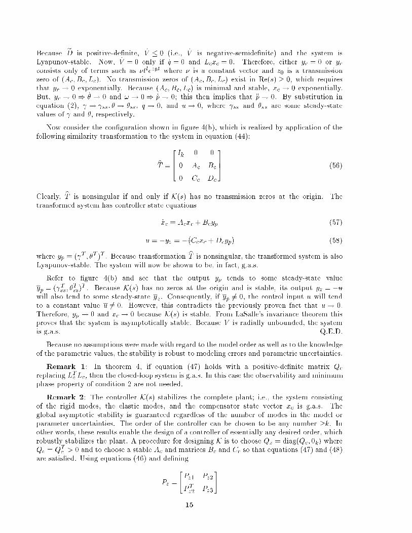
Because eD is positive-de�nite, _V � 0 (i.e., _V is negative-semide�nite) and the system isLyapunov-stable. Now, _V = 0 only if _q = 0 and Lcxc = 0. Therefore, either yr = 0 or yrconsists only of terms such as �tlez0t where � is a constant vector and z0 is a transmissionzero of (Ac; Bc; Lc). No transmission zeros of (Ac; Bc; Lc) exist in Re(s) � 0, which requiresthat yr ! 0 exponentially. Because (Ac; Bc; Lc) is minimal and stable, xc! 0 exponentially.But, yr ! 0) _� ! 0 and ! ! 0) _p! 0; this then implies that �p! 0. By substitution inequation (2), ! ss; �! �ss, q ! 0, and u! 0, where ss and �ss are some steady-statevalues of and �, respectively.

Now consider the con�guration shown in �gure 4(b), which is realized by application of thefollowing similarity transformation to the system in equation (44):

bT =

264 Ik 0 0

0 Ac Bc

0 Cc Dc

375 (56)

Clearly, bT is nonsingular if and only if K(s) has no transmission zeros at the origin. Thetransformed system has controller state equations

_xc = Acxc+Bcyp (57)

u = �yz = ��Ccxc+Dcyp

�(58)

where yp = ( T ; �T)T . Because transformation bT is nonsingular, the transformed system is alsoLyapunov-stable. The system will now be shown to be, in fact, g.a.s.

Refer to �gure 4(b) and see that the output yp tends to some steady-state value

yp = ( Tss; �Tss)

T . Because K(s) has no zeros at the origin and is stable, its output yz = �uwill also tend to some steady-state yz. Consequently, if yp 6= 0, the control input u will tendto a constant value u 6= 0. However, this contradicts the previously proven fact that u! 0.Therefore, yp! 0 and xc! 0 because K(s) is stable. From LaSalle's invariance theorem thisproves that the system is asymptotically stable. Because V is radially unbounded, the systemis g.a.s. Q.E.D.

Because no assumptions were made with regard to the model order as well as to the knowledgeof the parametric values, the stability is robust to modeling errors and parametric uncertainties.

Remark 1: In theorem 4, if equation (47) holds with a positive-de�nite matrix Qc

replacing LTc Lc, then the closed-loop system is g.a.s. In this case the observability and minimum

phase property of condition 2 are not needed.

Remark 2: The controller K(s) stabilizes the complete plant; i.e., the system consistingof the rigid modes, the elastic modes, and the compensator state vector xc is g.a.s. Theglobal asymptotic stability is guaranteed regardless of the number of modes in the model orparameter uncertainties. The order of the controller can be chosen to be any number �k. Inother words, these results enable the design of a controller of essentially any desired order, whichrobustly stabilizes the plant. A procedure for designing K is to choose Qz = diag(Qc; 0k) whereQc = QT

c > 0 and to choose a stable Ac and matrices Bc and Cc so that equations (47) and (48)are satis�ed. Using equations (46) and de�ning

Pz =

"Pz1 Pz2

PTz2 Pz3

#

15

where Pz1 is nc� nc and Pz3 is k � k, conditions 2 and 3 of theorem 4 can be expanded as

Pz1Ac+ATc Pz1+ Pz2Cc + CT

c PTz2 = �Qc

PTz2Ac+ Pz3Cc = 0

BTc Pz1+DT

c PTz2= 0

BTc Pz2+DT

c Pz3= I

9>>>>>>>=>>>>>>>;

(59)

In addition, Pz must be positive-de�nite. Because of the large number of free parame-ters (Ac; Bc; Cc; Dc;Qc), the use of equations (59) to obtain the compensator is generally notstraightforward. Another method is to use the s-domain equivalent of theorem 4. Theorem 5gives these equivalent conditions on K in the s-domain.

Theorem 5: The closed-loop system given by equations (21), (57), and (58) is g.a.s. if K(s)has no transmission zeros at s = 0, and K(s)=s is MSPR.

Proof: The proof can be obtained by a slight modi�cation of the results of reference 29 toshow that the theorem statement implies the conditions of theorem 4.

The condition that K(s)=s be MSPR is sometimes much easier to check than the conditionsof theorem 1. For example, let K(s) = diag[K1(s); : : : ;Kk(s)], where

Ki(s)= kis2+ �1is+ �0i

s2 + �1is + �0i(60)

A straightforward analysis shows that K(s)=s is MSPR if, and only if, ki, �0i, �1i, �0i, and �1iare positive for i = 1; 2; : : : ; k, and

�1i� �1i> 0 (61)

�1i�0i � �0i�1i > 0 (62)

For higher order Ki's, the conditions on the polynomial coe�cients are harder to obtain. Onesystematic procedure for obtaining such conditions for higher order controllers is the applicationof Sturm's theorem. (See ref. 27.) Symbolic manipulation codes can then be used to deriveexplicit inequalities. The controller design problem can be subsequently posed as a constrainedoptimization problem which minimizes a given performance function. However, the case offully populated K(s) has no straightforward method of solution and remains an area for futureresearch.

The following results, which address the cases with static dissipative controllers when theactuators have �rst- and second-order dynamics, are an immediate consequence of theorem 5and are stated without proof.

Corollary 5.1: For the static dissipative controller (eq. (22)), suppose that Gp and Gr arediagonal with positive entries denoted by subscript i, and actuators represented by the transferfunctionGAi(s) = ki=(s + ai) are present in the ith control channel. Then the closed-loop systemis g.a.s. if Gri > Gpi=ai (for i = 1; 2; : : : ; k).

Corollary 5.2: Suppose that the static dissipative controller also includes the feedback ofthe acceleration ya, that is,

u = �Gpyp� Gryr �Gaya

16

where Gp, Gr, and Ga are diagonal with positive entries. Suppose that the actuator dynamics

for the ith input channel are given by GAi(s) = ki=(s2+ �is+ �i) with ki, �i, and �i positive.

Then the closed-loop system is a.s. if

Gri

Gai� �i <

Gri

Gpi(i = 1;2; : : : ; k)

5.3.3. Realization of K as strictly proper controller. The controller K(s) (eqs. (57)and (58)) is not strictly proper because of the direct transmission term Dc. From a practicalviewpoint, a strictly proper controller is sometimes desirable because it attenuates sensor noise aswell as high-frequency disturbances. Furthermore, the most common types of controllers, whichinclude the linear quadratic Gaussian (LQG) controllers as well as the observer-pole placementcontrollers, are strictly proper; they have a �rst-order rollo�. In addition, the realization inequations (57) and (58) does not utilize the rate measurement yr. The following result statesthat K can be realized as a strictly proper controller wherein both yp and yr are utilized.

Theorem 6: The nonlinear plant with yp and yr as outputs is stabilized by thenc-dimensional controller K0 given by

_xc = Acxc+[Bc �AcL L ]

"yp

yr

#(63)

yc = Ccxc (64)

where Cc is assumed to be of full rank, and an nc� k (nc � k) matrix L is a solution of

Dc� CcL = 0 (65)

Proof: Consider the controller realization equations (57) and (58). Let

xc = xc+ Lyp (66)

where L is an nc� k matrix. The di�erentiation of equation (66), use of equations (57) and (58),and replacement of _yp with yr results in equation (63) and leads to

yc = Ccxc+(Dc� CcL)yp (67)

If L is chosen to satisfy equation (65), the strictly proper controller is given by equations (63)and (64). Equation (65) represents k2 equations in knc unknowns. If k < nc (i.e., thecompensator order is greater than the number of plant inputs) and Cc is of full rank, manypossible solutions exist for L. The solution which minimizes the Frobenius norm of L is

L = CTc

�CcC

Tc

��1Dc (68)

If k = nc, equation (68) gives the unique solution L = C�1c Dc.

6. Linear Single-Body Spacecraft

In this section, the case of a single-body exible spacecraft is considered, which is a specialcase of the systems discussed in section 5. The motivation for investigating this case separatelyis that a number of spacecraft belong to this class (e.g., exible space antennas). In addition, themathematical models for this class of spacecraft are linear, which permits the use of a variety of

17

controller synthesis techniques that are not available for nonlinear systems. However, the basicstability results for the linear case under static and dynamic dissipative compensation can beobtained as special cases of the stability results for nonlinear models. (Refer to section 5.)

6.1. Linearized Mathematical Model

The linearized mathematical model of the rotational dynamics of single-body exible spacestructure can be obtained by linearizing equation (2) about the zero steady state and is givenby cM�p+ bKp = BTu (69)

wherep =

��T; qT

�T � =(�; �; )T (70)

Here, � represents the 3� 1 attitude vector, q is the nq � 1 vector of elastic modal amplitudes

(nq = n� 3), cM is the positive-de�nite symmetric mass-inertia matrix (note that cM is constant

in this case), bK is the positive-semide�nite sti�ness matrix related to the exible degrees offreedom, u is the 3� 1 input torque vector, and B = [I3; 03�nq]. The system in equation (69)can be transformed into modal form by using transformation � = �p, where � is the eigenvector

matrix such that �TcM� = I and �T bK� = eC , a diagonal matrix. The resulting model is

�� + eC� = �TBTu =

"�T11

�T12

#u (71)

where �T11 and �

T12 are 3� 3 and nq � 3 matrices, respectively, and matrix eC is given by

eC = diag(03;�) (72)

where� = diag

�!21; !2

2; : : : ; !2nq

�(73)

in which !i (i = 1; 2; : : : ; nq) represent the elastic mode frequencies. The �rst three componentsof � correspond to rigid-body modes. The rigid-body modes are controllable if, and only if,�11 is nonsingular. Because one torque actuator is used for each of the X-, Y -, and Z-axes,�11 is nonsingular. Note that the mass-inertia matrix in this modal form is the 3� 3 identitymatrix. However, the model is customarily used in a slightly modi�ed form wherein the elasticmotion is superimposed on the rigid-body motion. (See ref. 4.) This can be achieved as follows.Suppose J = JT > 0 is the moment-of-inertia matrix of the spacecraft. Then, with the use ofthe transformation, � = �� where the transformation matrix � is given by

� =

"�T11J 03�nq

0nq�3 Inq�nq

#(74)

Equation (71) is transformed to

��� + eC�� ="�T11

�T12

#u (75)

Premultiplication of the above equation by ��1 yields

�� +��1eC�� =" J�1�T12

#u (76)

18

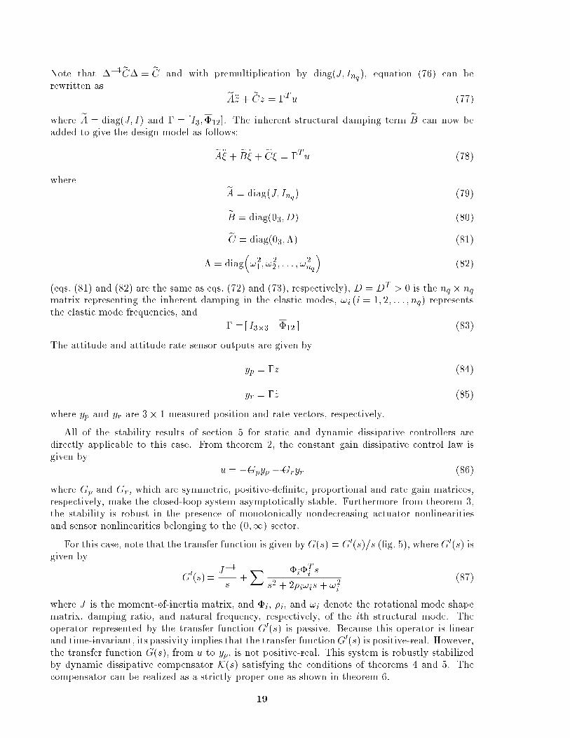
Note that ��1eC� = eC and with premultiplication by diag(J; Inq), equation (76) can berewritten as

eA�z + eCz = �Tu (77)

where eA = diag(J; I) and � = [I3;�12]. The inherent structural damping term eB can now beadded to give the design model as follows:

eA�� + eB _� + eC� = �Tu (78)

whereeA = diag

�J; Inq

�(79)

eB = diag(03;D) (80)

eC = diag(03;�) (81)

� = diag�!21; !

22; : : : ; !

2nq

�(82)

(eqs. (81) and (82) are the same as eqs. (72) and (73), respectively), D = DT > 0 is the nq � nqmatrix representing the inherent damping in the elastic modes, !i (i = 1; 2; : : : ; nq) representsthe elastic mode frequencies, and

� =[ I3�3 �12 ] (83)

The attitude and attitude rate sensor outputs are given by

yp = �z (84)

yr = �_z (85)

where yp and yr are 3� 1 measured position and rate vectors, respectively.

All of the stability results of section 5 for static and dynamic dissipative controllers aredirectly applicable to this case. From theorem 2, the constant gain dissipative control law isgiven by

u = �Gpyp �Gryr (86)

where Gp and Gr, which are symmetric, positive-de�nite, proportional and rate gain matrices,respectively, make the closed-loop system asymptotically stable. Furthermore from theorem 3,the stability is robust in the presence of monotonically nondecreasing actuator nonlinearitiesand sensor nonlinearities belonging to the (0;1) sector.

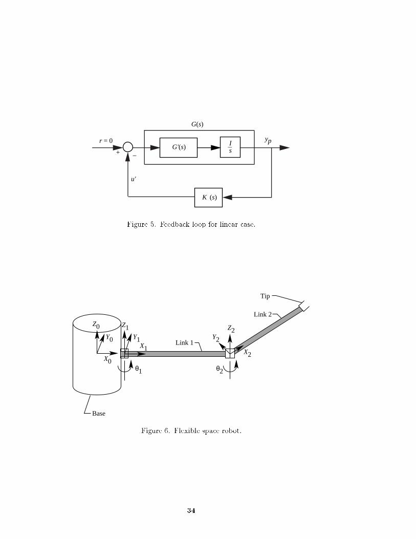
For this case, note that the transfer function is given byG(s) = G0(s)=s (�g. 5), where G0(s) isgiven by

G0(s)=J�1

s+X �i�

Ti s

s2+ 2�i!is+ !2i(87)

where J is the moment-of-inertia matrix, and �i, �i, and !i denote the rotational mode shapematrix, damping ratio, and natural frequency, respectively, of the ith structural mode. Theoperator represented by the transfer function G0(s) is passive. Because this operator is linearand time-invariant, its passivity implies that the transfer functionG0(s) is positive-real. However,the transfer function G(s), from u to yp, is not positive-real. This system is robustly stabilizedby dynamic dissipative compensator K(s) satisfying the conditions of theorems 4 and 5. Thecompensator can be realized as a strictly proper one as shown in theorem 6.

19

6.2. Optimal Dynamic Dissipative Compensator

The results of theorems 5 and 6 can be applied to check if a given model-based controller,such as an LQG controller, is dissipative (i.e., if it robustly stabilizes G(s)). In particular, thefollowing result is obtained.

Theorem 7: Consider the nkth-order LQG controller given by

_& = A&& +H

"yp

yr

#(88)

u = F& (89)

where A& is the closed-loop LQG compensator matrix

A& = A0� B0F +HC0 (90)

A0, B0, and C0 denote the design model matrices, and F and H are the regulator andestimator gain matrices, respectively. This controller robustly stabilizes the system if the rationalmatrix M(s)=s is MSPR where

M(s)= F (sI �A&)�1(H1+A&H2)+ FH2 (91)

and H1 and H2 denote the matrices consisting of the �rst three columns and the last threecolumns of H, respectively.

The theorem can be proved by using the transformation _ex = & �H2yp in equation (88).Although a given LQG controller will not be likely to satisfy the condition of theorem 7, thecondition can be incorporated as a constraint in the design process. The problem can be posed asone of minimizing a given LQG performance function with the constraint thatM(s)=s is MSPR.Also note that theorem 7 is not limited to an LQG controller but is valid for any observer-basedcontroller with control gain F and observer gain H. Another way of posing the design problemis to obtain the dissipative compensator which is closest to a given LQG design. The distancebetween compensators can be de�ned as either

1. The distance between the compensator transfer functions in terms of H2 or H1 norm ofthe di�erence or

2. The distance between the matrices used in the realization in terms of a matrix (i.e.,spectral or Frobenius) norm

For example, the dissipative compensator Ac and Cc matrices can be taken to be the LQG A&

and F matrices, respectively, and the compensator Bc and Dc matrices can be chosen tominimize � as follows while still satisfying the MSPR constraint:

� =

Bc �(H1+ A&H2)

Dc� FH2

2 or1

(92)

Thus the design method usually ends up as a constrained optimization problem.

7. Numerical Examples

Two numerical examples are given to demonstrate some of the results obtained in sections 4and 6. The �rst example consists of a conceptual nonlinear model of a spacecraft with two exiblearticulated appendages. The stability results for the nonlinear dissipative control law given in

20

section 4 are veri�ed by simulation. The second example addresses attitude control system designfor a large space antenna, which is modeled as a linear single-body structure. The objective of

the control system is to minimize a prescribed quadratic performance index. For this system, the

conventional LQG controller design was found to have stability problems due to unmodeled high-

frequency dynamics and parametric uncertainties. However, the dynamic dissipative controller

designed to minimize the quadratic performance function resulted in good performance with

guaranteed stability in the presence of both unmodeled dynamics and parametric uncertainties.

7.1. Two-Link Flexible Space Robot

The system shown in �gure 6 is used for validation of the theoretical results obtained in

section 4. The con�guration consists of a central body with two articulated exible links attached

to it and resembles a exible space robot. The central body is a solid cyinder 1.0 m in diameterand 2 m in height. Each link is modeled in MSC/NASTRAN1as a 3-m-long exible beam with

20 bar elements. The circular cross sections of the links are 1.0 cm in diameter resulting in

signi�cant exibility. The material chosen for the central body as well as the links has a mass

density of 2:568� 10�3 kg/m3 and modulus of elasticity E = 6:34� 109 kg/m2. The central-

body mass is 4030 kg and each link mass is 0.605 kg. The principal moments of inertia of the

central-body about local X-, Y -, and Z-axes are 1600, 1600, and 500 kg-m2, respectively. Each

link can rotate about its local Z-axis. The link moment of inertia about its axis of rotation is

1.815 kg-m2. The central body has three rotational degrees of freedom. As shown in �gure 6,

two revolute joints exist: one between the central-body and link 1 and another between links 1

and 2. The axes of rotation for revolute joints 1 and 2 coincide with the local Z-axes of links 1

and 2, respectively. Collocated actuators and sensors are assumed for each rigid degree of

freedom. Sensor measurements are also assumed to be available for the central-body attitude

(quaternions) and rates as well as revolute joint angles and rates.

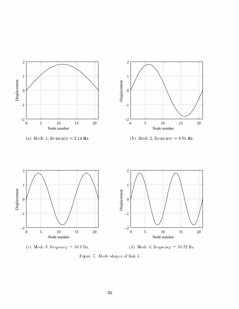
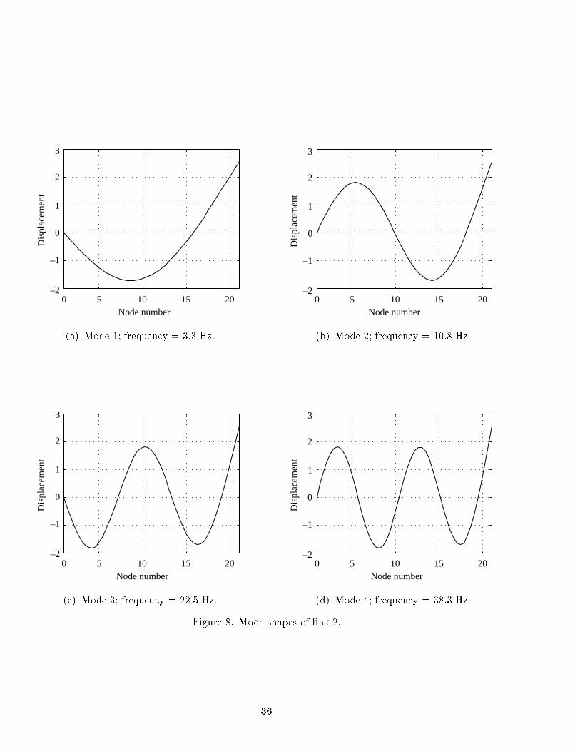
The �rst link was modeled as a exible beam with pinned-pinned boundary conditions; the

second link was modeled as a exible beam with pinned-free boundary conditions. For the

purpose of simulation, the �rst four bending modes in the local XY -plane were considered for

each link (i.e., the system has �ve rigid rotational degrees of freedom and eight exible degrees

of freedom, four for each link). The modal data were obtained from MSC/NASTRAN. The

mode shapes and the frequencies for links 1 and 2 are shown in �gures 7 and 8, respectively. A

complete nonlinear simulation was obtained with DADS2, a commercially available software.

A rest-to-rest maneuver was considered to demonstrate the control law. The initial con�gu-

ration was equivalent to (�=4)-rad rotation of the entire spacecraft about the global X-axis and

0.5-rad rotation of the revolute joint 2. The objective of the control law was to restore the zero

state of the system. A nonlinear dissipative controller (eq. (13)) was used to accomplish the

task. Because there are no known techniques to date for the synthesis of such controllers, the

selection of controller gains was based on trial and error. Based on several trials, the following

gains were found to give the desirable response: Gp1 = diag(500; 500; 500), Gp2 = diag(50; 50),

and Gr = diag(500; 275; 270; 100; 100). As the system begins motion, all members move relative

to one another, and dynamic interaction exists between members. Complete nonlinear and cou-

pling e�ects are incorporated in the simulation. The Euler parameter responses are shown in

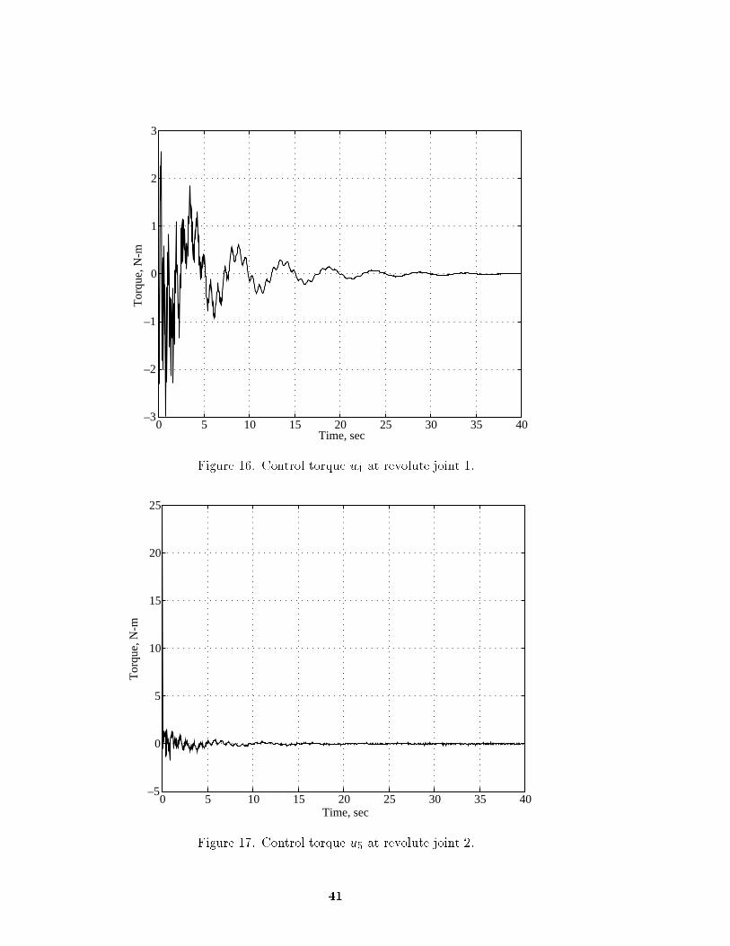
�gures 9 and 10, and the joint angle displacements for the revolute joints 1 and 2 are shown in

�gure 11. The joint displacements decay asymptotically and are nearly zero within 15 sec. The

tip displacements with respect to globalX-, Y -, and Z-axes are shown in �gures 12 and 13. Note

that the manipulator tip reaches its desired x position in about 15 sec, whereas the desired y and

z positions are reached in about 35 sec. These responses e�ectively demonstrate the stability

1 Trademark of The MacNeal-Schwendler Corp., Los Angeles, CA 90041.2 Trademark of Computer Aided Design Software, Inc., Oakdale, IA 52319.

21

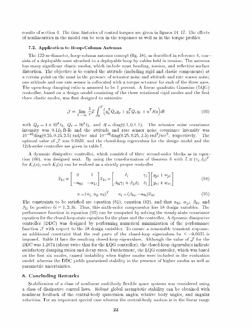
results of section 4. The time histories of control torques are given in �gures 14{17. The e�ectsof nonlinearities in the model can be seen in the responses as well as in the torque pro�les.

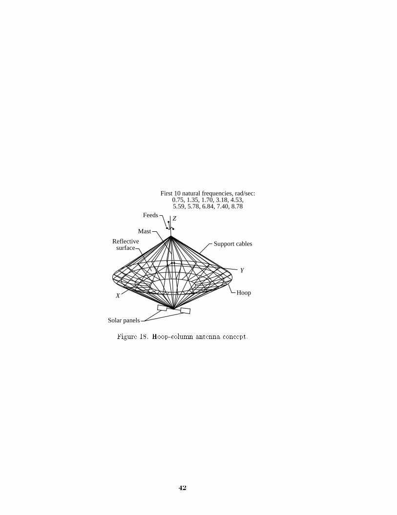
7.2. Application to Hoop-Column Antenna

The 122-m-diameter, hoop-column antenna concept (�g. 18), as described in reference 4, con-

sists of a deployable mast attached to a deployable hoop by cables held in tension. The antenna

has many signi�cant elastic modes, which include mast bending, torsion, and re ective surface

distortion. The objective is to control the attitude (including rigid and elastic components) at

a certain point on the mast in the presence of actuator noise and attitude and rate sensor noise;

one attitude and one rate sensor is collocated with a torque actuator for each of the three axes.The open-loop damping ratio is assumed to be 1 percent. A linear quadratic Gaussian (LQG)

controller, based on a design model consisting of the three rotational rigid modes and the �rst

three elastic modes, was �rst designed to minimize

J = limT!1

1

TE

ZT

0

�yTpQpyp+ yTrQryr + uTRu

�dt (93)

with Qp = 4� 108I3, Qr = 108I3, and R = diag(0:1; 0:1;1). The actuator noise covariance

intensity was 0:1I3 ft-lb and the attitude and rate sensor noise covariance intensity was

10�10diag(0:25; 0:25; 2:5) rad/sec and 10�10diag(0:25; 0:25; 2:5) rad2/sec2, respectively. The

optimal value of J was 0.6036, and the closed-loop eigenvalues for the design model and the

12th-order controller are given in table I.

A dynamic dissipative controller, which consisted of three second-order blocks as in equa-

tion (60), was designed next. By using the transformation of theorem 6 with L = ( i; �i)T

for Ki(s), each Ki(s) can be realized as a strictly proper controller

_xki=

"0 1

��0i ��1i

#xki+

"�i i

�0i i+ �1i�i �i

#"ypi+ wpi

yri+ wri

#(94)

u =(u1; u2; u3)T ui =(�0i;��0i)xki (95)

The constraints to be satis�ed are equation (61), equation (62), and that �0i, �1i, �0i, and

�1i be positive (i = 1; 2; 3). Thus, this sixth-order compensator has 18 design variables. The

performance function in equation (93) can be computed by solving the steady-state covariance

equation for the closed-loop state equation for the plant and the controller. A dynamic dissipative

controller (DDC) was designed by performing numerical minimization of the performance

function J with respect to the 18 design variables. To ensure a reasonable transient response,

an additional constraint that the real parts of the closed-loop eigenvalues be � �0:0035 is

imposed. Table II lists the resulting closed-loop eigenvalues. Although the value of J for the

DDC was 1.2674 (about twice that for the LQG controller), the closed-loop eigenvalues indicate

satisfactory damping ratios and decay rates. Furthermore, the LQG controller, which was based

on the �rst six modes, caused instability when higher modes were included in the evaluation

model, whereas the DDC yields guaranteed stability in the presence of higher modes as well as

parametric uncertainties.

8. Concluding Remarks

Stabilization of a class of nonlinear multibody exible space systems was considered using

a class of dissipative control laws. Robust global asymptotic stability can be obtained with

nonlinear feedback of the central-body quaternion angles, relative body angles, and angular

velocities. For an important special case wherein the central-body motion is in the linear range

22

while all the appendages undergo unlimited motion, global asymptotic stability under a linear

dissipative control law was proved. Furthermore, the robust stability was showed to be preserved

in the presence of a broad class of actuator and sensor nonlinearities and a class of actuator

dynamics.

A class of dynamic dissipative controllers was introduced and was proved to provide global

asymptotic stability for the case where the central-body motion is small. Dynamic dissipative

controllers o�er more design freedom than static dissipative controllers and, therefore, can

achieve better performance and noise attenuation.

Linear single-body spacecraft represent a special case of nonlinear multibody spacecraft, and

therefore, the robust stability results are directly applicable to this case.

All the stability results presented are valid in spite of unmodeled modes and parametric

uncertainties; i.e., the stability is robust to model errors. The results have a signi�cant practical

value because the mathematical models of such systems usually have substantial inaccuracies,

and the actuation and sensing devices have nonlinearities.

Design of dissipative controllers to obtain optimal performance is, as yet, an unsolved

problem, especially for the nonlinear case. Future work should address the development of

systematic methods for the synthesis of both nonlinear and linear, static and dynamic, dissipative

controllers.

NASALangley Research Center

Hampton, VA 23681-0001

December 23, 1994

23

Appendix

Mathematical Model Derivation and System Properties

The steps involved in the derivation of equations of motion (eq. (2)) are outlined in thisappendix. The details of the derivation of the mass-inertia matrix M(p) and the sti�ness

matrix eK are not included but can be found in reference 14.

Kinetic Energy

The kinetic energy of the system represented in �gure 1 is given by

T =1

2_pTM(p) _p (A1)

where M(p) is the con�guration-dependent symmetric and positive-de�nite mass-inertia matrixof the system and p is the vector of the generalized coordinates.

Potential Energy

Generally, the potential energy of a system has many sources (e.g., elastic displacementor thermal deformation). The deformations due to thermal e�ects are not considered in theformulation in this paper; however, they can easily be included in the formulation if desired.Thus, the potential energy is assumed to consist of the contribution only from the strain energydue to elastic deformation. Also, the materials under consideration are assumed to be isotropicin nature and to obey Hooke's law.

If eK is the sti�ness matrix of the system, then the potential energy of the system is given by

V =1

2qT eKq

where q is the vector of the exible degrees of freedom. If the matrix K is de�ned as

K =

"0k�k 0k�(n�k)

0(n�k)�keK(n�k)�(n�k)

#

then the potential energy of the system can be rewritten in terms of the generalized variable pas

V =1

2pTKp (A2)

Equations of Motion

From equations (A1) and (A2), the Lagrangian of the system is formed as

L = T � V

For convenience, L can be rewritten in the indicial notation as

L = T � V =1

2

Xi;j

Mij _pi _pj � V (A3)

The Euler-Lagrange equations for the system can then be derived from

d

dt

�@L

@ _pk

��

@L

@pk= Fk (A4)

24

where Fk are generalized forces from the nonconservative force �eld. From evaluation of thederivatives,

@L

@ _pk=Xj

Mkj _pj (A5)

and

d

dt

�@L

@ _pk

�=Xj

Mkj�pj +Xj

Mkj _pj

=Xj

Mkj�pj +Xi;j

@Mkj

@pi_pi _pj (A6)

Also@L

@pk=

1

2

Xi;j

@Mij

@pk_pi _pj �

@V

@pk(A7)

Thus, the Euler-Lagrange equations can be written as

Xj

Mkj�pj +Xi;j

�@Mkj

@pi�

1

2

@Mij

@pk

�_pi _pj �

@V

@pk= Fk (k = 1; 2; : : : ; n) (A8)

By interchanging the order of summation and taking advantage of symmetry,

Xi;j

�@Mkj

@pi

�_pi _pj =

1

2

Xi;j

�@Mkj

@pi+@Mki

@pj

�_pi _pj (A9)

Hence, Xi;j

�@Mkj

@pi�

1

2

@Mij

@pk

�_pi _pj =

Xi;j

1

2

�@Mkj

@pi+@Mki

@pj�

@Mij

@pk

�_pi _pj (A10)

The terms

Cijk =1

2

�@Mkj

@pi+@Mki

@pj�

@Mij

@pk

�(A11)

are known as Christo�el symbols. For each �xed k, note that Cijk = Cjki. Also,

@V

@pk= Kkjpj (A12)

Finally, the Euler-Lagrange equations of motion can be written as

Xj

Mkj�pj +Xi;j

Cijk _pi _pj +Dkj _p+Kkjpj = Fk (k = 1; 2; : : : ; n) (A13)

where D is the inherent structural damping matrix and D _p is the vector of nonconservativeforces.

Of the four terms on the left side of equation (A13), the �rst term involves second derivativesof the generalized coordinates p. The second term consists of centrifugal terms (e.g., _p2i ) andCoriolis terms (e.g., _pi _pj, i 6= j). In general, the coe�cients Cij are functions of p. The thirdterm involves only the �rst derivatives of p and corresponds to the dissipative forces due to

25

inherent damping. The fourth term, which involves only p, arises from the di�erentiation of thepotential energy.

In matrix-vector notation, equation (A13) can be written as

M(p)�p+ C(p; _p) _p+D _p+Kp = F (A14)

The k; jth element of the matrix C(p; _p) is de�ned as

Ckj =

nXi=1

cijk(p) _pi

=

nXi=1

1

2

�@Mkj

@pi+@Mki

@pj�

@Mij

@pk

�_pi (A15)

An important property of the systems whose equations of motion are given by equation (A14)is derived next. This property is pivotal to the stability results obtained in sections 4 and 5.

Theorem A1: The matrix S = _M(p)� 2C(p; _p) is skew-symmetric.

Proof: The k; jth element of the time derivative of the mass-inertia matrix _M(p) is givenby the chain rule as

_Mkj =

nXi=1

@Mkj

@pi_pi (A16)

Therefore, the k; jth component of S = _M � 2C is given by

Skj =_Mkj � 2Ckj

=

nXi=1

�@Mkj

@pi�

�@Mkj

@pi+@Mki

@pj�

@Mij

@pk

��_pi

=

nXi=1

�@Mij

@pk�

@Mki

@pj

�_pi (A17)

Because the inertia matrix is symmetric (i.e., Mij = Mji), the interchange of the indices kand j in equation (A17) results in

Sjk = �Skj (A18)

This completes the proof. Q.E.D.

Theorem A1 can be used to prove that the system given by equations (2) has the importantproperty of passivity as de�ned in reference 3.

Theorem A2: The input-output map from u to yr is passive, i.e., with zero initial conditions,

Z T

0

yTr (t)u(t)� 0 (8T � 0) (A19)

for all u(t) belonging to the extended Lebesgue space Lk2e.

Proof: Premultiplication of both sides of equations (2) by _pT and integration result in

Z T

0

h_pTM(p)�p+ _pTC(p; _p) _p+ _pTD _p+ _pTKp

i=

Z T

0

yTr u dt (A20)

26

Note thatd

dt

h_pTM(p) _p

i= 2_pTM(p)�p+ _pT _M(p) _p (A21)

Application of theorem A1 and simpli�cation yields

1

2_pT(T )M [p(T )] _p(T )+

ZT

0

_pTD _pdt+1

2pT(T )Kp(T )=

ZT

0

yTr u dt (A22)

Because the left side of equation (A22) is nonnegative for all T � 0, this gives the required result.Q.E.D.

27

References

1. Asrar, Ghassem; and Dokken, David Jon, eds.: 1993 Earth Observing System Reference Handbook. NASA

NP-202, 1993.

2. General Electric Co.: Upper AtmosphereResearchSatellite (UARS) Project DataBook. NASACR-193176, 1987.

3. Desoer, Charles A.; and Vidyasagar, M.: Feedback Systems: Input-Output Properties. Academic Press, 1975.

4. Joshi, S. M.: Control of Large Flexible Space Structures. Volume 131 of LectureNotes inControl and InformationSciences, M. Thoma and A. Wyner, eds., Springer-Verlag, 1989.

5. Meirovitch, Leonard: Methods of Analytical Dynamics. McGraw-Hill BookCo., Inc., 1970.

6. Takegaki, M.; and Arimoto, S.: A New FeedbackMethod for Dynamic Control of Manipulators. J. Dyn. Syst.,

Meas. & Control, vol. 103, June 1981, pp. 119{125.

7. Koditschek, Dan: Natural Motion for RobotArms. Proceedings of the 23rdConference on Decision and Control,

IEEE, Dec. 1984, pp. 733{735.

8. Spong, MarkW.; and Vidyasagar, M.: Robot Dynamics and Control. JohnWiley& Sons, Inc., 1989.

9. Vidyasagar, M.: Nonlinear Systems Analysis. Prentice-Hall, Inc., 1993.

10. Wen, John T.; and Bayard, David S.: New Class of Control Laws for Robotic Manipulators. Int. J. Control,

vol. 47, May 1988, I|Nonadaptive Case, pp. 1361{1385, and II|Adaptive Case, pp. 1387{1406.

11. Paden, Brad; and Panja, Ravi: Globally Asymptotically Stable `PD+' Controller for Robot Manipulators. Int.

J. Control, vol. 47, June 1988, pp. 1697{1712.

12. Paden, Brad; Riedle, Brad; and Bayo, Eduardo: Exponentially Stable Tracking Control for Multi-Joint

Flexible-Link Manipulators. Proceedings of the 9th American Control Conference, Volume 1, IEEE, 1990,

pp. 680{684.

13. Juang, Jer-Nan; Wu, Shih-Chin; Phan, Minh; and Longman, Richard W.: Passive Dynamic Controllers for

Nonlinear Mechanical Systems. J. Guid., Control, & Dyn., vol. 16, no. 5, Sept.{Oct. 1993, pp. 845{851.

14. Kelkar, Atul G.: Mathematical Modeling of a Class of Multibody Flexible Space Structures. NASA TM-109166,

1994.

15. Greenwood, Donald T.: Principles of Dynamics. Prentice-Hall, Inc., 1965.

16. Wen, John Ting-Yung; and Kreutz-Delgado, Kenneth: The Attitude Control Problem. IEEE Trans. Autom.

Control, vol. 36, Oct. 1991, pp. 1148{1162.

17. Kane, T. R.: Solution of Kinematical Di�erential Equations for a RigidBody. J. Appl. Mech., vol. 4, Mar. 1973,pp. 109{113.

18. Ickes, B. P.: A NewMethod for Performing Digital Control SystemAttitude Computations Using Quaternions.AIAA J., vol. 8, 1970, pp. 13{17.

19. Harding, C. F.: Solution to Euler's Gyrodynamics. J. Appl. Mech., vol. 31, June 1964, pp. 325{328.

20. Haug, Edward J.: Computer Aided Kinematics and Dynamics of Mechanical Systems. Allyn and Bacon, 1989.

21. Benhabib, R. J.; Iwens, R. P.; and Jackson, R. L.: Stability of Large Space Structure Control Systems UsingPositivity Concepts. J. Guid. & Control, vol. 4, no. 5, Sept.{Oct. 1981, pp. 487{494.

22. McLaren, M. D.; and Slater, G. L.: Robust Multivariable Control of Large Space Structures Using Positivity.J. Guid., Control, & Dyn., vol. 10, no. 4, July{Aug. 1987, pp. 393{400.

23. Slater, G. L.; andMcLaren, M. D.: EstimatorEigenvalue Placement inPositive Real Control. J. Guid., Control,

& Dyn., vol. 13, Jan.{Feb. 1990, pp. 168{175.

24. Popov, V. M.: Hyperstability of Control Systems. Springer-Verlag, 1973.

25. Lozano-Leal, Rogelio; and Joshi, SureshM.: Strictly Positive Real Transfer Functions Revisited. IEEE Trans.

Autom. Control, vol. 35, no. 11, Nov. 1990, pp. 1243{1245.

26. Joshi, S. M.; Maghami, P. G.; and Kelkar, A. G.: Dynamic Dissipative Compensator Design for Large Space

Structures. A Collection of Technical Papers, AIAA Guidance, Navigation and Control Conference, Volume 1,

Aug. 1991, pp. 467{477. (Available as AIAA-91-2650-CP.)

28

27. Van Valkenburg, M. E.: Introduction to ModernNetwork Synthesis. JohnWiley & Sons, Inc., 1960.

28. Anderson, B. D. O.: A System Theory Criterion for Positive Real Matrices. SIAM J. Control, vol. 5, no. 2,

May 1967, pp. 171{182.

29. Joshi, SureshM.; and Gupta, Sandeep: Robust Stabilization of Marginally Stable Positive-Real Systems. NASA

TM-109136, 1994.

29

Table I. Closed-Loop Eigenvalues for LQG Controller

Regulator Estimator

�0:0238� 0:0542i �0:0240� 0:0544i�0:0721� 0:0964i �0:0720� 0:0965i�0:0754� 0:1000i �0:0725� 0:0963i�0:3169� 0:8108i �0:4050� 0:7703i�0:2388� 1:3554i �0:3334� 1:3333i�0:3375� 1:7030i �0:5104� 1:6562i

Table II. Closed-Loop Eigenvalues for

Dynamic Dissipative Controller

�0:0035� 0:0194i�0:0183� 0:0458i�0:0160� 0:0502i�0:3419� 0:5913i�0:7179� 0:6428i�0:8479� 0:5653i�0:6482� 1:6451i�0:4536� 2:1473i�0:3764� 2:5522i

30

Central body

Branch Branch Branch

Figure 1. Multibody system.

31

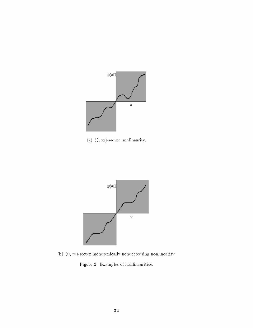
ψ(ν)

ν

(a) (0;1)-sector nonlinearity.

ψ(ν)

ν

(b) (0;1)-sector monotonically nondecreasing nonlinearity.

Figure 2. Examples of nonlinearities.

32

u'

Is

K (s)

+ –

ypr = 0 Nonlinearplant

yr

Figure 3. Feedback closed-loop con�guration.

Nonlinear

plant

K (s)

+ –

yrr = 0 u

.yz = v v = ycI

s

(a) Compensator with rate input.

+ –

Nonlinear

plant

K (s)

yrr = 0 u

yz yp Is

(b) Compensator with position input.

Figure 4. Rearrangement of feedback loops.

33

u'

+ –

K (s)

ypr = 0 IsG'(s)

G(s)

Figure 5. Feedback loop for linear case.

Link 1

Link 2

Tip

Base

θ1 θ2

X2

Z2Y2

X1

Z1Y1

Z0

Y0

X0

Figure 6. Flexible space robot.

34

5 10 15 20–2

–1

0

1

2

Node number

Dis

plac

emen

t

0

(a) Mode 1; frequency = 2.14 Hz.

5 10 15 20–2

–1

0

1

2

Node number

Dis

plac

emen

t0

(b) Mode 2; frequency = 8.58 Hz.

5 10 15 20–2

–1

0

1

2

Node number

Dis

plac

emen

t

0

(c) Mode 3; frequency = 19.3 Hz.

5 10 15 20–2

–1

0

1

2

Node number

Dis

plac

emen

t

0

(d) Mode 4; frequency = 34.32 Hz.

Figure 7. Mode shapes of link 1.

35

5 10 15 20–2

–1

0

1

3

Node number

Dis

plac

emen

t

0

2

(a) Mode 1; frequency = 3.3 Hz.

5 10 15 20Node number

Dis

plac

emen

t0

–2

–1

0

1

3

2

(b) Mode 2; frequency = 10.8 Hz.

5 10 15 20Node number

Dis

plac

emen

t

0–2

–1

0

1

3

2

(c) Mode 3; frequency = 22.5 Hz.

5 10 15 20Node number

Dis

plac

emen

t

0–2

–1

0

1

3

2

(d) Mode 4; frequency = 38.3 Hz.

Figure 8. Mode shapes of link 2.

36

0 5 10 15 20 25 30 35 40–.10

–.05

0

.05

.10

.15

.20

.25

.30

.35

.40

Time, sec

α 1

Figure 9. Euler parameter �1.

0 5 10 15 20 25 30 35 40–1.5

–1.0

–.5

0

.5

1.0 × 10–3

Time, sec

α 2, α3

α2α3

Figure 10. Euler parameters �2 and �3.

37

0 5 10 15 20 25 30 35 40–.1

0

.1

.2

.3

.4

.5

Time, sec

θ 1, θ2, r

ad

θ1θ2

Figure 11. Revolute joint angular displacement.

38

0 5 10 15 20 25 30 35 406.15

6.20

6.25

6.30

6.35

6.40

6.45

6.50

Time, sec

Tip

dis

plac

emen

t, m

Figure 12. Tip displacement (x coordinate).

zy

0 5 10 15 20 25 30 35 40–.2

0

.2

.4

.6

.8

1.0

Time, sec

Tip

dis

plac

emen

t, m

Figure 13. Tip displacement (y and z coordinates).

39

0 5 10 15 20 25 30 35 40–200

–150

–100

–50

0

50

100

Time, sec

Tor

que,

N-m

Figure 14. Control torque u1.

0 5 10 15 20 25 30 35 40–3

–2

–1

0

1

2

3

4

Time, sec

Tor

que,

N-m

u2u3

Figure 15. Control torques u2 and u3.

40

0 5 10 15 20 25 30 35 40–3

–2

–1

0

1

2

3

Time, sec

Tor

que,

N-m

Figure 16. Control torque u4 at revolute joint 1.

0 5 10 15 20 25 30 35 40–5

0

5

10

15

20

25

Time, sec

Tor

que,

N-m

Figure 17. Control torque u5 at revolute joint 2.

41

Solar panels

Reflectivesurface

Mast

Support cables

Y

X Hoop

Feeds

First 10 natural frequencies, rad/sec:0.75, 1.35, 1.70, 3.18, 4.53,5.59, 5.78, 6.84, 7.40, 8.78

Z

Figure 18. Hoop-column antenna concept.

42

REPORT DOCUMENTATION PAGEForm Approved

OMB No. 0704-0188

Public reporting burden for this collection of information is estimated to average 1 hour per response, including the time for reviewing instructions, searching existing data sources,gathering and maintaining the data needed, and completing and reviewing the collection of information. Send comments regarding this burden estimate or any other aspect of thiscollection of information, including suggestions for reducing this burden, to Washington Headquarters Services, Directorate for Information Operations and Reports, 1215 Je�ersonDavis Highway, Suite 1204, Arlington, VA 22202-4302, and to the O�ce of Management and Budget, Paperwork Reduction Project (0704-0188), Washington, DC 20503.

1. AGENCY USE ONLY(Leave blank) 2. REPORT DATE 3. REPORT TYPE AND DATES COVERED

May 1995 Technical Paper

4. TITLE AND SUBTITLE

A Class of Stabilizing Controllers for Flexible Multibody Systems

6. AUTHOR(S)

Suresh M. Joshi, Atul G. Kelkar, and Peiman G. Maghami

7. PERFORMING ORGANIZATION NAME(S) AND ADDRESS(ES)

NASA Langley Research CenterHampton, VA 23681-0001

9. SPONSORING/MONITORING AGENCY NAME(S) AND ADDRESS(ES)

National Aeronautics and Space AdministrationWashington, DC 20546-0001

5. FUNDING NUMBERS

WU 233-01-01-05

8. PERFORMING ORGANIZATION

REPORT NUMBER

L-17413

10. SPONSORING/MONITORING

AGENCY REPORT NUMBER

NASA TP-3494

11. SUPPLEMENTARY NOTES

Joshi and Maghami: Langley Research Center, Hampton, VA; Kelkar: Langley Research Center (NationalResearch Council Research Associate), Hampton, VA.

12a. DISTRIBUTION/AVAILABILITY STATEMENT 12b. DISTRIBUTION CODE

Unclassi�ed{UnlimitedSubject Category 18Availability: NASA CASI (301) 621-0390

13. ABSTRACT (Maximum 200 words)

This paper considers the problem of controlling a class of nonlinear multibody exible space systems consistingof a exible central body to which a number of articulated appendages are attached. Collocated actuators andsensors are assumed, and global asymptotic stability of such systems is established under a nonlinear dissipativecontrol law. The stability is shown to be robust to unmodeled dynamics and parametric uncertainties. Fora special case in which the attitude motion of the central body is small, the system, although still nonlinear,is shown to be stabilized by linear dissipative control laws. Two types of linear controllers are considered:static dissipative (constant gain) and dynamic dissipative. The static dissipative control law is also shown toprovide robust stability in the presence of certain classes of actuator and sensor nonlinearities and actuatordynamics. The results obtained for this special case can also be readily applied for controlling single-bodylinear exible space structures. For this case, a synthesis technique for the design of a suboptimal dynamicdissipative controller is also presented. The results obtained in this paper are applicable to a broad class ofmultibody and single-body systems such as exible multilink manipulators, multipayload space platforms, andspace antennas. The stability proofs use the Lyapunov approach and exploit the inherent passivity of suchsystems.

14. SUBJECT TERMS 15. NUMBER OF PAGES

Multibody systems control; Flexible space structures 43

16. PRICE CODE

A0317. SECURITY CLASSIFICATION 18. SECURITY CLASSIFICATION 19. SECURITY CLASSIFICATION 20. LIMITATION

OF REPORT OF THIS PAGE OF ABSTRACT OF ABSTRACT

Unclassi�ed Unclassi�ed Unclassi�ed

NSN 7540-01-280-5500 Standard Form 298(Rev. 2-89)Prescribed by ANSI Std. Z39-18298-102