a cfd study of a urea based scr mixing system at volvo...
TRANSCRIPT

A CFD Study of the Urea Supply, Droplet
Breakup and Mixing in a Pipe Upstream of a
SCR Catalyst A design application under development at Volvo Penta Master´s thesis in the Master´s program Innovative and Sustainable Chemical Engineering
EMELIE SAMUELSSON
SARA HOLMBERG
Department of Chemical and Biochemical Engineering
Division of Chemical Engineering
CHALMERS UNIVERSITY OF TECHNOLOGY
Gothenburg, Sweden, 2013

Cover: The front page shows the urea-water spray and two static mixers from an upstream position.
A CFD Study of the Urea Supply, Droplet Breakup and Mixing in a Pipe Upstream of a SCR Catalyst
A design application under development at Volvo Penta EMELIE SAMUELSSON
SARA HOLMBERG
© EMELIE SAMUELSSON, SARA HOLMBERG, 2013.
Department of Chemical and Biological Engineering
Chalmers University of Technology
SE-412 96 Göteborg
Sweden
Telephone + 46 (0)31-772 100

i
Preface This Master of Science thesis has been performed by Emelie Samuelsson and Sara Holmberg, both
students at the Innovative and Sustainable Chemical Engineering Master’s program at Chalmers
University of Technology, Gothenburg, Sweden. All work has been equally divided and executed in
an equal manner. The work was performed in collaboration with FS Dynamics, Volvo Penta and the
Department of Chemical and Biochemical Engineering at Chalmers University of Technology, during
the spring 2013. The supervisor of the Master of Science thesis was Dr. Jonas Edman at FS Dynamics
and examiner was Assistant Professor Ronnie Andersson at Chalmers University of Technology.
Acknowledgements First, we would like to thank our supervisor Jonas Edman for all help and support during the project.
We would also like to express our gratitude to Sture Wingård and Ulrika Grimfeldt for their
enthusiasm and useful input to the project. We would like to thank Assistant Professor Ronnie
Andersson and Professor Bengt Andresson for the rewarding discussions regarding difficulties in
analyzing our results. We would also like to thank Tony Persson for giving us feedback on the report
and all other members in the CFD master thesis group within FS Dynamics for the pleasant meetings
and helpful discussions during the project. We would also like to thank everyone at the department at
Volvo Penta for an enjoyable environment and for lending us their computers when we needed it most.
Finally, we would like to express our gratitude to our families and friends for their support and love in
both rainy and sunny days.

ii
Abstract The reduction of NOX emissions from diesel engines by urea SCR (Selective Catalytic Reduction) is a
well-established technique. The European standard emission levels are continuously tightened which
put high demands on the aftertreatment system. In order to improve the mixing capacity and the
breakup of the urea spray in the SCR system, static mixers can be installed. In this thesis a worst case
scenario is studied where a pipe based mixing system is used upstream of the SCR resulting in limited
time and space for evaporation and mixing. The aim was to study the mixing of the urea spray and the
exhaust gas in the mixing pipe by means of CFD simulations. The interaction between the spray, the
mixers and the turbulent flow field has been studied. Methods for evaluating the SCR performance
through CFD simulations were also improved and developed.
The simulations were performed in STAR-CCM+ v.8.02.008 and the studied geometries were pre-
processed in ANSA v.14.0. An engine operating point that has shown low NOX reduction was used for
the simulations. The geometry studied include the mixing pipe upstream of the SCR catalyst which
was complemented with one, two or three mixers at different positions in order to determine which
configuration that gives the most favorable results. Different injector strategies have also been
investigated. In order to capture the behavior of the spray due to the pulsating injector, transient
simulations were performed. A sensitivity analysis of the turbulence model, mesh density and inlet
velocity profile was performed. The single phase flow was modeled using the Realizable k-ε model
and the multiphase flow was modeled using the Euler-Lagrange framework.
Two new measurement methods were developed; Urea Conversion and Stoichiometric Area Index
(SAI), in order to better estimate the mixing performance and NOX reduction. It was shown that the
urea conversion is strongly dependent on the droplet size and the residence time of the droplets. The
SAI is dependent on both the urea conversion and the mixing performed by the bulk flow. Further it
was concluded that introducing mixers in the system increases both the urea conversion and SAI which
results in increased NOX reduction. The highest urea conversion was obtained for the case with three
mixers at 50, 100, and 150 mm downstream of the injector. The highest SAI was reached when two
injectors were used. Since SAI reflects the possible NOX conversion this case was considered to be the
most favorable in this study. It has potential to reach an even higher SAI if an injector with a lower
mass flow is used.
iii
Contents 1 Introduction ..................................................................................................................................... 1
1.1 Background ............................................................................................................................. 1
1.2 Purpose .................................................................................................................................... 2
1.3 Constraints ............................................................................................................................... 2
2 Diesel combustion and Regulations ................................................................................................ 3
2.1 Combustion and emissions ...................................................................................................... 3
2.2 NOX aftertreatment techniques ................................................................................................ 3
2.3 SCR ......................................................................................................................................... 4
2.3.1 SCR types ........................................................................................................................ 4
2.3.2 Urea decomposition ......................................................................................................... 4
2.3.3 SCR surface chemistry .................................................................................................... 5
2.3.4 SCR catalyst .................................................................................................................... 6
2.3.5 Unwanted reaction paths ................................................................................................. 6
3 Sprays .............................................................................................................................................. 7
3.1 Atomizer .................................................................................................................................. 7
3.1.1 Pressure Atomizer ........................................................................................................... 7
3.2 The simulated injector ............................................................................................................. 7
3.3 Droplet size distribution (Rosin-Rammler) ............................................................................. 9
3.4 Droplet evaporation ................................................................................................................. 9
3.5 Spray-wall interactions ............................................................................................................ 9
4 CFD simulations ............................................................................................................................ 10
4.1 Single phase modeling ........................................................................................................... 10
4.1.1 Modeling the turbulence ................................................................................................ 10
4.1.2 Realizable k- ε model .................................................................................................... 10
4.1.3 Two-layer All y+ Wall Treatment ................................................................................. 11
4.1.4 SST k-ω turbulence model ............................................................................................ 11
4.2 Multiphase modeling ............................................................................................................. 12
4.2.1 The Euler-Lagrange model ............................................................................................ 12
5 Important parameters for the SCR performance............................................................................ 16
5.1 Effect of the upstream turbocharger ...................................................................................... 16
5.2 Mixing ................................................................................................................................... 16
5.2.1 Turbulent mixing ........................................................................................................... 16
5.2.2 Static mixers .................................................................................................................. 17
5.3 Ammonia storage in the catalyst ........................................................................................... 18
5.4 Different injection strategies ................................................................................................. 18

iv
6 CFD method .................................................................................................................................. 19
6.1 Geometry ............................................................................................................................... 19
6.2 Mesh ...................................................................................................................................... 19
6.2.1 Spatial and temporal discretization schemes ................................................................. 21
6.3 Measuring convergence ......................................................................................................... 21
6.4 Evaluating SCR performance ................................................................................................ 21
6.4.1 Droplet size and distribution ......................................................................................... 21
6.4.2 Urea conversion ............................................................................................................. 21
6.4.3 Turbulent length scale ................................................................................................... 22
6.4.4 Uniformity Index (UI) ................................................................................................... 22
6.4.5 Difference in mole relation and Stoichiometric Area Index (SAI) ................................ 22
6.5 Simulation set-up ................................................................................................................... 23
6.5.1 Case study ...................................................................................................................... 23
6.5.2 Mixer and injector configurations ................................................................................. 23
6.5.3 Boundaries ..................................................................................................................... 23
7 Sensitivity analysis ........................................................................................................................ 25
7.1 Realizable k-ε vs. SST turbulence model .............................................................................. 25
7.2 Analysis of mesh independence ............................................................................................ 25
7.3 Analysis of sensitivity to the upstream turbocharger ............................................................ 25
8 Results and discussion ................................................................................................................... 26
8.1 Characterization of the system .............................................................................................. 26
8.1.1 Droplet size and distribution ......................................................................................... 26
8.1.2 Urea conversion ............................................................................................................. 27
8.1.3 Turbulent length scale ................................................................................................... 27
8.1.4 Uniformity Index ........................................................................................................... 28
8.1.5 Difference in mole relation and Stoichiometric Area Index (SAI) ................................ 29
8.1.6 Important parameters for evaluating the SCR performance .......................................... 31
8.2 The effect of the positions of two mixers and of introducing a third mixer to the system .... 31
8.2.1 Urea conversion and droplet size distribution ............................................................... 32
8.2.2 Stoichiometric Area Index (SAI) ................................................................................... 34
8.3 The effect of injector position, number and injection type .................................................... 35
8.3.1 Urea conversion and droplet size distribution ............................................................... 35
8.3.2 Stoichiometric Area Index (SAI) ................................................................................... 36
9 Conclusions ................................................................................................................................... 37
10 Future studies ............................................................................................................................ 38
10.1 Proposed design for further investigation of the system ....................................................... 38

v
10.2 Proposed improvement to evaluating methods ...................................................................... 38
11 Bibliography .............................................................................................................................. 40
A Appendix – Calculation of rpm for the swirling flow .................................................................. 42
B Appendix – Calculation of droplet evaporation, Stoke’s number and thermal response time ...... 43
Droplet evaporation time and length ................................................................................................. 43
Stoke’s number .................................................................................................................................. 43
Thermal response time ...................................................................................................................... 45
C Appendix – Residence time and mixer pressure drop ................................................................... 47


1
1 Introduction
1.1 Background Nitrogen oxides or NOX is an undesired pollutant in the exhaust gases produced in the combustion
process of a diesel engine due to non-ideal conditions [1]. The European emission standards regulates
the allowed emission level of NOX from diesel engines and this level has decreased significantly
during the last decade and is supposed to decrease even more in the near future. The non-road diesel
engines produced at Volvo Penta contain a SCR system to reduce the amount of NOX in the exhaust
gases. In such system, ammonia (NH3) is used as a reducing agent to convert NOX into nitrogen gas
(N2) and water (H2O) [2]. Since NH3 is an unhealthy chemical even at low concentrations, urea is used
as a NH3 source [3]. In a urea based SCR system a solution of urea (32,5wt %) and water called
AdBlue is injected into the hot exhaust gases through atomization. The water has to evaporate before
urea may decompose to NH3 [4]. Naturally, to obtain a high NOX conversion over the catalyst, it is of
importance to achieve a high conversion of urea and a uniform mixture between NOX and NH3. In
order to achieve this, static mixers can be installed to enhance the turbulence and break up the spray
into smaller droplets.
Computational Fluid Dynamics (CFD) has been an important tool for designing and developing
exhaust gas aftertreatment systems in the automotive industry. The process of evaluating the SCR
performance experimentally by measuring the NH3 concentration at the inlet of the SCR catalyst is a
difficult task that is both expensive and time consuming. However, numerical methods and
computational technologies are developed rapidly which enables CFD simulations to predict the
atomization and chemical reactions taking place in an SCR system along with the flow mixing. Hence,
by predicting the flow uniformity through CFD simulations the time for the development progression
has declined significantly [5].
Volvo Penta produces diesel engines for many different applications with varying space limitations.
This means that for some applications there may be sufficient space to obtain both a high conversion
of urea and a good mixing of NH3 and NOX before the catalyst inlet is reached. However, in some
applications the space is very limited, meaning that the mixing system where the injection of AdBlue,
decomposition of urea and mixing takes place has to be very compact. Regardless of the application,
the amount of released NOX has to be within the allowed level and preparation has to be done for the
future when the allowed level is supposed to be reduced even more.
This study is based on a worst case scenario where the mixing system upstream of the SCR catalyst is
a short and straight pipe which is a challenge in terms of urea conversion and flow mixing due to the
short residence time. To obtain an enhanced SCR performance the mixing pipe in this study is
complemented with static mixers that can create turbulence which favours flow mixing and can
interact with the spray by reducing the droplet size. The performance of different designs has been
evaluated by predicting the outcome through CFD simulations.
This master thesis is based on a former study at Volvo Penta that analyzed the effect of including one
mixer into a mixing-system. How the results changed when the position of the mixer was varied was
also investigated in the former study. Based on the earlier gained knowledge this study aims to deepen
the understanding of the system and further analyze possible improvements by introducing additional
mixers.

2
1.2 Purpose The aim of this thesis is to study the mixing phenomena of urea and exhaust gases in the mixing pipe
which is located upstream of the SCR catalyst. The interaction between the spray, the turbulent flow
field and the mixer elements is studied. The results are assessed as trends in order to get a better
knowledge of how the system works and what modifications that will improve the results in terms of
urea conversion and the mixing performance. The methods for evaluating the system performance are
analyzed and developed in order to get a better estimation of the NOX conversion.
1.3 Constraints Since there are very little experimental data available, the results from the study cannot be
validated. A comparison between two turbulence models has been performed in order to
analyze the sensitivity on the result between suitable turbulence models.
The reactions modeled in the study are limited to the urea decomposition in the bulk phase due
to both technical and practical limitations.
To evaluate the NOX conversion, the mole relation between the involved species over a cross-
section at inlet of the SCR catalyst is studied.
The exhaust gas is simulated as air since the surface chemistry is not modeled.
The geometry used in the simulations is cut 5 cm into the catalyst in order to make the
simulations less computationally expensive.
The possible modifications of the mixing pipe are physically limited by a flex pipe positioned
between the mixing pipe and the SCR inlet. It is not possible to position any mixer inside the
flex pipe.
A simplified geometry of the system was used, where flanges located at the beginning and end
of the flex pipe were removed.

3
2 Diesel combustion and Regulations
2.1 Combustion and emissions Diesel engines combusts hydrocarbons and the products at ideal conditions are carbon dioxide (CO2)
and water (H2O). Consequently, the exhaust gas from the engine will primarily consist of CO2, H2O
and unused air from the combustion. If the conditions are not ideal, pollutants are produced in addition
to CO2 and H2O. Some of these pollutants have undesirable impact on the environment and/or health.
Common pollutants are unburned hydrocarbons (HC), carbon monoxide (CO), nitrogen oxides (NOX)
and particulate matter (PM) [1]. Nitrogen oxide emissions (NOX) include nitric oxide (NO) and
nitrogen dioxide (NO2).
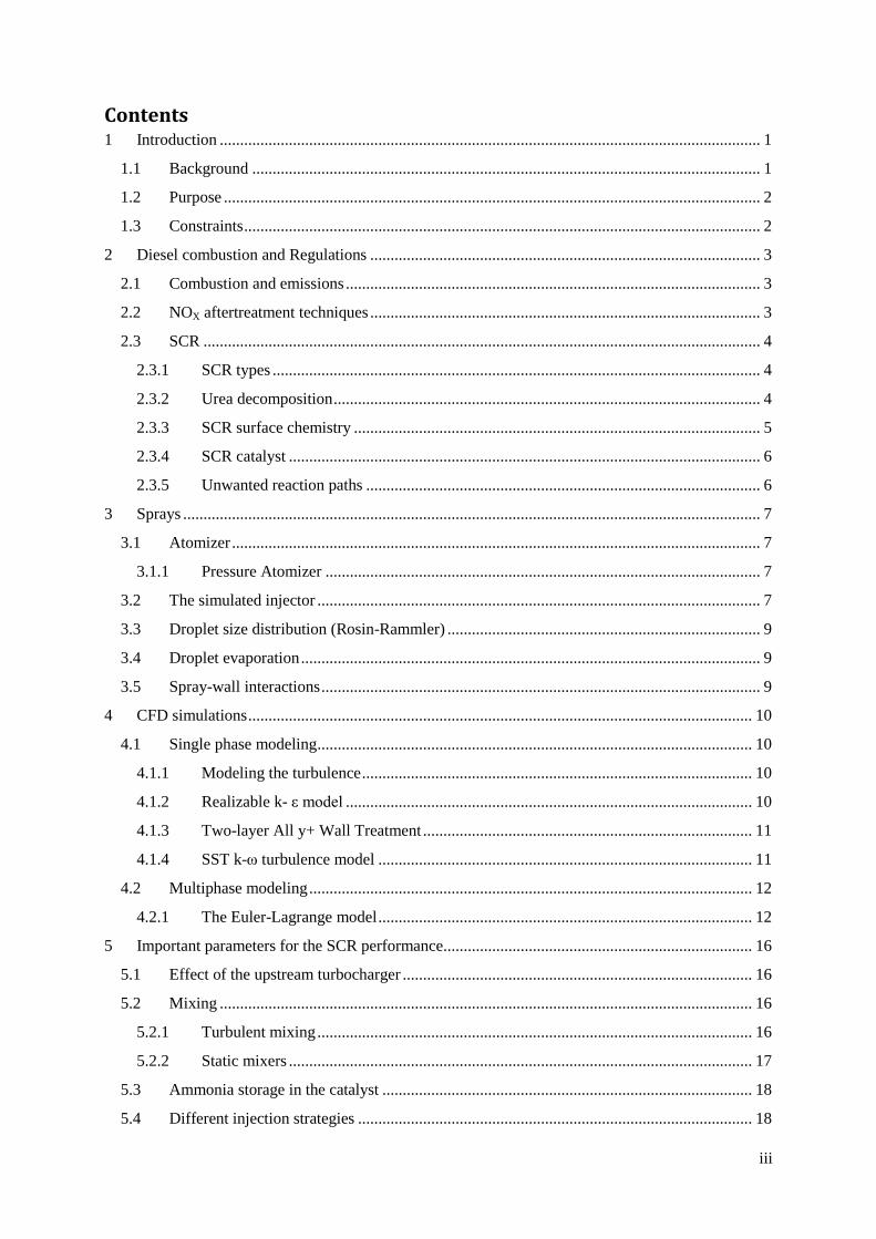
For non-road diesel engines there are European emission standards to regulate the allowed released
emission limit, which are known as Stage . The allowed NOX level for engines between 130 and
560 kW during the period 1999-2014 is shown in Figure 1. The first legislation for emissions from
non-road diesel engines in Europe was implemented in two steps; Stage was introduced in 1999 and
Stage from 2001 to 2004 depending on the power output of the engine. The emission limits
specified in these two stages were so called engine-out limits meaning the emissions prior to any
exhaust aftertreatment device. Stage , which is further divided into Stage and Stage was
implemented in 2006-2008 and 2011-2013 respectively and the standards in Stage will be
introduced 2014. These standards additionally include an emission limit for ammonia. In Stage a
limit of 0.025 g/kWh of particulate matter were introduced and to reach this limit the use of a
particulate filter after the engine was anticipated. The upcoming Stage has a significantly lower
limit of NOX which likewise is expected to require a NOX aftertreatment device to be developed [6].
Figure 1: The levels of the European standards Stage I-VI and the year introduced.
2.2 NOX aftertreatment techniques In order to meet the upcoming standard levels concerning NOX discharge, some aftertreatment device
is required. There are different technologies for aftertreatment of NOX and some of the most common
techniques available today are:
Lean NOX catalysts where hydrocarbons are added to the exhaust gases reduce NOX and forms
nitrogen, carbon dioxide and water. The main disadvantage with these types of catalysts is the
relatively low NOX conversion (10-20%). This technology is therefore not seen as a possible
technology to meet the future standards [2].
0
1
2
3
4
5
6
7
8
9
10
1999: Stage I 2002: Stage II 2006: Stage IIIA 2011: Stage III B 2014: Stage IV
NO
X [
g/kW
h]

4
NOX adsorbers which can be used together with Lean NOX catalysts and adsorb NOX at low
temperatures where the Lean NOX catalyst have poor performance. The adsorbed NOX is then
released at temperatures that promote the reaction with hydrocarbons [2]. However, NOX
adsorbers are receptive to sulfur poisoning meaning that the adsorption of sulfur causes
irreversible catalyst deactivation. This is the main reason for not using this type of catalyst in
diesel engines [3].
Plasma-assisted catalyst where non-thermal plasma is used to generate radicals that can
reduce or oxidize the NO molecules [7]. Since oxygen is present in the exhaust gases, the
oxidation reaction will be the main reaction and NO may be oxidized to NO2 and the reduction
of NOX will therefore be low. Since the technology is relatively novel, further research is
required for evaluating future use in aftertreatment applications for diesel engines and it is not
commercially used at the moment [8].
Selective catalytic reduction (SCR) is used in the Volvo Penta applications and is described in
2.3.
2.3 SCR In a SCR system, ammonia (NH3) is used as a reducing agent to convert NOX into nitrogen gas (N2)
and water (H2O). The main advantage with this system is the high NOX conversions (90% or higher).
The disadvantages involves the space required for the catalyst, high capital- and operating costs,
formation of other emissions (NH3 slip) and formation of undesirable compounds which may lead to
catalyst masking and deactivation. The NH3 slip can be controlled by installing an oxidation catalyst
after the SCR system. Although the SCR system has some drawbacks, the technology has been chosen
by the majority of the diesel engine manufactures, due to absence of better options to meet the
European standards [2].
2.3.1 SCR types
There are three possible ways to introduce NH3 to the system; anhydrous NH3, aqueous NH3 or an
aqueous urea solution that decomposes to NH3. Ammonia is irritating to skin, eyes and mucous
membranes even at low concentrations. The potential risk associated concerning storing and handling
the gaseous NH3 is significant and consequentially it is not commonly used. Hydrous NH3 has a lower
vapor pressure than the anhydrous resulting in decreased consequences in case of an accident. In order
to avoid direct handling of both anhydrous and aqueous NH3, urea is often used as an NH3 source [3].
2.3.2 Urea decomposition
In a urea SCR system, a urea-water solution often referred to as AdBlue is sprayed into the hot exhaust
gases. The AdBlue solution contains 32.5wt % urea and 67.5wt % water. The generation of NH3 in the
SCR system is preceded in three steps as described in reactions (1)-(3). In the first reaction, water is
evaporated from the AdBlue droplet and the urea is decomposed to NH3 and iso-cyanic acid (HNCO)
though the termohydrolysis in the second reaction. The state of the urea after the water has evaporated
is not fully understood according to Birkhold et al. [4] since some authors report the urea to be in
gaseous phase and others that the urea is in solid state.
Evaporation of water from the droplets [4]:
(1)
Thermolysis of urea into NH3 and iso-cyanic acid [4]:
(2)
5
HNCO in gas phase is quite stable but can easily be converted to NH3[4] and carbon dioxide through
the hydrolysis reaction if the temperature is sufficiently high (400° C or higher) or on the surface of
metal oxides at lower temperatures [9].
Hydrolysis of iso-cyanic acid [4]:
(3)
At favorable conditions, one mole urea will consequentially give two moles of NH3. Since the urea is
the only NH3 source in the SCR, the decomposition is an important step for the overall performance.
Both NH3 and HNCO will react with NOX at the catalyst surface (HNCO reacts as described in (3) and
then with NOX) and these two species will hereby be called the active substance. It has been proved by
Yim et al. [9] that the time required to fully decompose the urea is decreased as temperature is
increased and vice versa.
The urea thermolysis and HNCO hydrolysis are modeled assuming reacting species in gas phase and
the kinetics are specified according to a study of Yim et al. [9]. The kinetics of the thermal
decomposition of urea, reaction (2) and (3), has been investigated suggesting that the thermolysis of
urea into the active substance is independent on the presence of a catalyst. In contrast, the reaction rate
constant of the hydrolysis is larger in the presence of a catalyst than without indicating that the
hydrolysis can be accelerated by a catalyst. The reaction rate constants for the thermolysis of urea, k1,
and hydrolysis of iso-cyanic acid, k2´, in absence of a catalyst are presented by Yim et al. [9] as
(
)
(
)
where the activation energies are given in J mol-1
K-1
and the pre-exponential factors are given in s-1
.
The constant is a product of the reaction rate constant and the concentration of water vapour. The
concentration of water is high in the exhaust gas stream and will hences not vary. Further depends
highly on the temperature, resulting in high activation energy and a high temperature is needed to
induce the reaction. However, the reaction rate of the hydrolysis is increased on the surface of metal
oxides i.e. on the catalyst surface at lower temperatures [9].
2.3.3 SCR surface chemistry
There are four key reactions taking place in the SCR [10]:
(4)
(5)
(6)
(7)
Due to the fact that usually 90% of the NOX in diesel exhaust gas is NO, reaction (4) is the main
reaction of the SCR. Reaction (5) and (7) are slower than the main reaction. Reaction (6) is on the
other hand faster than the main reaction which means that equimolar amount of NO and NO2 is
favorable for a high conversion of NOX [10]. Due to both technical and practical limitations the surface
chemistry is not modeled. However, it is assumed that equation (4) is the most significant reaction and
that all formed active substance will react with NOX and that the NOX only consist of NO.
6
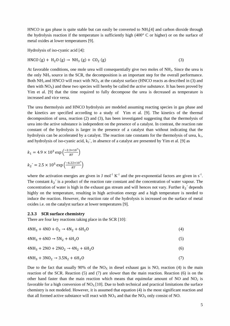
2.3.4 SCR catalyst
The reactions described in section 2.3.3 takes place on the catalyst surface at active sites which have a
relatively even distribution over the surface. The catalyst used in an SCR system is a monolithic
catalyst. A monolith consists of square channels running through the whole catalyst substrate, as
shown schematically in Figure 2. Monoliths can be prepared entirely from the specific catalyst
material or may include some inert material e.g. metallic or ceramic that act as support material, with a
catalytic layer applied on the walls of the channels [11]. Since the catalyst is divided into channels
there will not be any significant mixing after the gas flow has entered the catalyst. Hence, it is
important to distribute the active substance evenly over the SCR catalyst inlet and thereby making it
available in all channels. This emphasizes the importance of reaching a uniform mixture prior to the
catalyst inlet.
Figure 2: A schematic figure of a monolith catalyst. The substrate is divided into several channels where the reaction
takes place on the catalyst surface.
2.3.5 Unwanted reaction paths
At high temperatures, above 400°C, NH3 may react to nitrous oxide at the catalyst surface and at even
higher temperatures the NH3 may be oxidized, reaction (8) and (9) respectively [12]. Such
temperatures are reached at high work load of the engine.
(8)
(9)
Since these reactions consume NH3, the maximum conversion of NOX is limited by the amount of
reacted NH3 [10]. The formation of nitrous oxide also contributes to the global warming which is
another reason for avoiding this reaction path [12].
During some conditions, uncompleted decomposition of urea can cause formation of undesired high
molecular weight by-products which may, at certain conditions, form a solid deposit on the surfaces of
the urea SCR system. As a consequence of the incomplete decomposition of urea and formation of
deposits, NH3 formation is also lowered and the catalyst surface may be affected giving a decreased
NOX reduction efficiency. The formation of solid deposits from by-products is mainly dependent on
the temperature. In studies made by Xu et. al [13] solid deposits in the SCR has been reported at
temperatures below 300°C. At temperatures above 350°C, the majority of the deposits vaporize [13].
Temperatures below 300°C is reached when the engine has a relatively low work load and the exhaust
gas stream is not heated to higher temperature.
HNCO plays an important role in many of the routes for by-product formation, both as reactant to
form biuret and for further polymerization. A rapid hydrolysis of iso-cyanic acid is favorable since it
will decrease the formation of its possible by-products. Examples of undesired by-products are biuret
that can react further to cyaunic acid, ammelide, ammeline and melamine [14].

7
3 Sprays The AdBlue solution is sprayed into the flow of exhaust gases upstream of the catalyst. The
atomization of liquids is a common process unit operation where a bulk fluid is transformed into a
spray system. The main intention with atomization processes is to maximize the gas-liquid interface
since all transport processes are directly dependent upon this surface area and the exchange between
the phases will improve with an increased surface. The exchange between the phases in a spray system
increases by several orders of magnitude compared to the case where the liquid is not disintegrated
through atomization [15].
3.1 Atomizer The atomization process itself is the method for breakup of the fluid and produces the resulting spray
structure. The principle used is different in different cases and is dependent on the properties of the
liquid that is to be atomized. Viscosity, surface tension and density are properties of importance which
may vary significantly between different materials. It can be said that the type of the atomizer used in
a specific purpose is dependent on:
The liquid material properties
The liquid material throughput
The required spray characteristics
3.1.1 Pressure Atomizer
The atomizer used in most technical applications is the pressure atomizer [15] with a plain-orifice
nozzle which is used in the SCR system at Volvo Penta. In a pressure atomizer a pressurized liquid is
forced through a small opening (orifice) into a gas at lower pressure and the plain-orifice nozzle
produces a full cone spray. The liquid will disintegrate to droplets as a result of the velocity difference.
This type of atomizer is typically used for low viscosity liquids [15]. For plane-orifice pressure
nozzles the most important feature for the atomization is the dimension of this opening. The finest
disintegration is reached when the orifice is small. However, the smaller it is, the more difficult it is to
keep the opening free from foreign particles. This means that there has to be a trade-off when choosing
the orifice size. Due to this, the minimum size of the orifice is usually limited to approximately 0.3
mm [16]. One drawback with the pressure atomizer is naturally the need of a pressurized liquid but
also that the droplets size produced is relatively uneven and the practicable mass flow rate is low [15].
3.2 The simulated injector The type of injector used in the simulations is a “solid cone” with a spray angle of 42°, i.e. angle b in
Figure 3. The principle direction of the spray diverge 50° from a straight injection, i.e. angle a in
Figure 3.

8
Figure 3: A schematic figure of injector for the AdBlue spray injection. The principle direction of the spray diverge
50° from a straight injection (a=50°) where the straight injection refers to an injection in the normal direction of the
mixing pipe wall. The spray angle b is 42°.
In the studied Volvo Penta application, the injector work at a frequency of 4 Hz. This means that urea
is injected four times per second at the maximum injection rate of 6.3 kg/h (1.75 g/s). The required
mass flow of urea is dependent upon the exhaust gas flow, which varies with the power output of the
engine. The total required amount urea per second should then equal the amount injected four times in
one second. The time for each injection pulse has to be calculated for each studied power output of the
engine. For example if 1 g/s of urea is needed, the injector should inject urea for 0.143 seconds four
times when the rate is 1.75 g/s. This type of injection curve is shown in Figure 4.
The injector is simulated as a point where droplets enter the domain with a frequency of 4 Hz and a
direction that diverge 50° from a straight injection. The droplet diameters are determined by the Rosin
Rammler distribution function described in chapter 3.3. Additionally, the mass flow rate, number of
parcels, droplet temperature, mass fractions of the species (urea and water) and the velocity magnitude
was specified for the injector.
Figure 4: Urea is injected with a frequency of 4 Hz and to get a mass flow of 1 g urea/s the injection time will be 0.143
s. The required amount urea varies with the exhaust gas flow and will be different for each power output.
0 0.1 0.2 0.3 0.4 0.5 0.6 0.7 0.8 0.9 10
0.2
0.4
0.6
0.8
1
1.2
1.4
1.6
1.8
2
Time [s]
Mass f
low
[kg/s
]
Injection curve
AdBlue spray b
a
90°
Injector
Pipe wall

9
3.3 Droplet size distribution (Rosin-Rammler) To describe the droplet sizes of the spray an empirical droplet size distribution function may be used.
There are several empirical functions for achieving a droplet size distribution and the choice of
function depends significantly on the disintegration mechanism for the situation. One function that has
been widely used (and is used in the spray simulations of this study) is the Rosin-Rammler distribution
which may be expressed as shown in equation (10).
𝑄 (𝐷𝑝
𝑋)𝑞 (10)
In this expression, 𝑄 represents the portion of the total volume holding drops with a diameter less than
. The exponent is a measure of the spread in size and a higher value means that the spray is more
uniform, set to 1.5 in the simulations. is the reference diameter which in the simulations is set to 93
µm [16].
3.4 Droplet evaporation There has to be a concentration difference in vapor between the droplet surface and the continuous
phase for the evaporation to take place. In most cases the continuous phase surrounding the droplet is
assumed to be a binary mixture of the gas and the droplet vapor [17]. The rate of the evaporation
process will be determined by the droplet size, temperature, pressure, material properties of the
surrounding gas and relative velocity between the phases. One common way to describe steady-state
evaporation i.e. when the droplet has reached the wet-bulb temperature that corresponds to the current
conditions, is the so called D2 law stated in equation (11) [16].
𝜆𝑡 (11)
where is the initial droplet diameter, is the droplet diameter at time 𝑡 and 𝜆 represents the
evaporation constant [16]. The evaporation constant may be defined through equation (12).
𝜆 4𝑆ℎ𝜌𝑐𝐷
𝜌𝑝 𝑚𝑓𝐴,𝑠 𝑚𝑓𝐴,∞ (12)
Where is the Sherwood number, is an average density for the binary mixture, is the density
for the dispersed phase (droplets), is the diffusion coefficient and 𝑚𝑓𝐴 is the mass fraction of species
A (vapor from the droplets) where and indicates at the droplet surface and in the free stream
respectively. This means that the evaporation constant will not be constant when the conditions of the
surrounding gas changes. However in many applications this may be an acceptable approximation
[17].
3.5 Spray-wall interactions The interaction between the spray and the wall involves complex mechanisms since the outcome of an
impinging droplet depends on several parameters including properties of the droplets, the surrounding
gas and the wall [4]. Accordingly, there are several different outcomes from an impinging droplet
which may be summarized by adhesion, rebound, spread, splash, rebound with break-up and break-up
[18]. These possible outcomes and conditions that determine which course of event is the most likely
to occur are further discussed in chapter 4.2.1.3.

10
4 CFD simulations The simulations have been executed in STAR-CCM+ v.8.02.008. In the following section all models
that have been used in the single and multiphase simulations performed in this thesis are described.
The theory described in this section is based on the textbook Computational Fluid Dynamics for
Engineers [19] and STAR-CCM+ Theory Guide [20].
4.1 Single phase modeling This section describes the flow characteristics and how these are modeled in the single phase
simulations. The single phase flow i.e. the exhaust gas flow and the evaporated NH3 is modeled as an
ideal gas mixture in all simulations of this study.
4.1.1 Modeling the turbulence
A turbulent flow of a fluid can be described as a random and chaotic motion and it is a degenerative
process. The large turbulence structures disintegrate into successively smaller structures until the small
structures have reached a minimum size and the energy is dissipated into heat. Hence, the turbulence
will die relatively quick if no energy is supplied to the system.
Turbulent flows are unsteady in nature, implying that the flow properties are functions of time. To
solve the dynamics of such unsteady flows a lot of computational power is required which makes it
impractical for industrial applications. Most models therefore solves for mean quantities of the flow.
An unsteady flow is therefore in these cases a flow where the statistical mean flow properties vary
with time. The turbulent flow in this case can be simulated as steady state since each power output is
approximated as steady state, hence the mean properties of the flow does not vary in time. The
realizable k-ε model and SST k-ω model, which are described in the following sections, was used to
model the turbulent flow and a second order upwind discretization scheme was applied and is further
described in section 6.2.1.
4.1.2 Realizable k- ε model
The Realizable k-ε model is a Reynolds Average Navier-Stokes (RANS) model based on the
Boussinesq approximation which is described in [19]. It is a two-equation model taking both turbulent
velocity and length scale into account. Transport equations are used to describe these variables
resulting in that both the turbulence production and dissipation may have different local rates.
In the realizable k-ε model the turbulent kinetic energy, k, is modeled by equation (13) which is a
transport equation for k.
𝜕𝑘
𝜕𝑡 ⟨𝑈𝑗⟩
𝜕𝑘
𝜕𝑥𝑗 𝜈 [(
𝜕⟨𝑈𝑖⟩
𝜕𝑥𝑗
𝜕⟨𝑈𝑗⟩
𝜕𝑥𝑖)
𝜕⟨𝑈𝑖⟩
𝜕𝑥𝑗] 𝜀
𝜕
𝜕𝑥𝑗[(𝜈
𝜈𝑇
𝜎𝑘)
𝜕𝑘
𝜕𝑥𝑗] (13)
i ii iii iv v
where the different terms describes
i. Accumulation of k
ii. Convection of k by mean velocity
iii. Production of k
iv. Dissipation of k
v. Diffusion of k
To close this equation the energy dissipation rate, ε, and the turbulent viscosity, , is needed. The
dissipation (ε) is modeled with another transport equation and the general form for this is stated in
equation (14).

11
𝜕𝜀
𝜕𝑡 ⟨𝑈𝑗⟩
𝜕𝜀
𝜕𝑥𝑗
𝜕
𝜕𝑥𝑗[(𝜈
𝜈𝑇
𝜎𝜀)
𝜕𝜀
𝜕𝑥𝑗] 𝐶𝜀 𝜀 𝐶𝜀
𝜀
𝑘+√𝑣𝜀 (14)
i ii iii iv v
where the different terms is describing
i. Accumulation of ε
ii. Convection of ε by mean velocity
iii. Diffusion of ε
iv. Production of ε
v. Dissipation of ε
The turbulent viscosity is then determined through
𝜈 𝐶𝜇𝑘2
𝜀 (15)
𝐶𝜇 is a variable determined from an equation. The four closure coefficients in above equations; 𝐶𝜀 ,
𝐶𝜀 , 𝜀 and 𝑘 are assumed to be constant even though they may vary slightly for different flows.
The realizable k-ε model is valid for most engineering applications. It is advantageous to use since it is
relatively robust, economical in terms of computational power and easy to apply. Compared to the
standard k-ε model it can handle swirling flows and flow separation because of a modification in the k
equation (14) which prevents the normal stresses to become negative. However it is not as stable as the
standard k-ε. Another disadvantage is the assumption that the turbulent viscosity is isotropic which
means that the convection and diffusion of the Reynolds stresses are not solved.
4.1.3 Two-layer All y+ Wall Treatment
The Realizable k-ε model was used alongside with the two-layer approach which is one method for
resolving the viscous sublayer. The computation is split into two layers. In the layer closest to the wall,
ε and is quantified as functions of the distance from the wall. The values of ε that is identified in
the near wall region are smoothly blended with the values of ε that is calculated far away from the
wall. However the equation for k is solved for the entire flow.
Additionally to the two-layer approach, the all y+ wall treatment in STAR CCM+ was applied. This is
a wall treatment that combines the high y+ wall treatment in regions with coarse mesh and the low y+
treatment in regions with fine mesh. In the high y+ wall treatment it is assumed that the cells near the
wall lies within the logarithmic section of the boundary layer. The low y+ wall treatment assumes that
the viscous sub-layer is accurately resolved and is therefore only valid for turbulence with low
Reynolds-numbers. The all y+ treatment also enables realistic solutions for meshes with intermediate
resolution i.e. when the cell near the wall lies within buffer region of the boundary layer in the near
wall region.
4.1.4 SST k-ω turbulence model
In order to analyze the sensitivity of the solution the SST k-ω turbulence model was used for the
simulation. It works well for separating flows and many authors recommend it as the first choice of
turbulence model. The model is based on a combination of both k-ε and k-ω models using the first one
in the free stream and the latter one in the near wall region. In the original k-ω turbulence model the
specific dissipation rate ω is used as a length-determining parameter instead of ε. The equation used to
model k is
𝜕𝑘
𝜕𝑡 ⟨𝑈𝑗⟩
𝜕𝑘
𝜕𝑥𝑗 [(
𝜕⟨𝑈𝑖⟩
𝜕𝑥𝑗
𝜕⟨𝑈𝑗⟩
𝜕𝑥𝑖)
𝜕⟨𝑈𝑖⟩
𝜕𝑥𝑗]
𝜕
𝜕𝑥𝑗[(
𝑇
𝜎𝑘)
𝜕𝑘
𝜕𝑥𝑗] (16)

12
where the different terms describes the same as in the k equation for the k-ε model, equation (13). ω is
modeled by
𝜕
𝜕𝑡 ⟨𝑈𝑗⟩
𝜕
𝜕𝑥𝑗
𝑘 [(
𝜕⟨𝑈𝑖⟩
𝜕𝑥𝑗
𝜕⟨𝑈𝑗⟩
𝜕𝑥𝑖)
𝜕⟨𝑈𝑖⟩
𝜕𝑥𝑗]
𝜕
𝜕𝑥𝑗[(
𝑇
𝜎 )
𝜕
𝜕𝑥𝑗] (17)
and the turbulent viscosity is calculated through
𝑘
(18)
The k- turbulence model is able to generate better result than the k-ε model in the near wall regions
due to the fact that k and ε must go to zero at correct rates at low Re numbers. This is because the
dissipation in the equation for ε contains ε2/k. The All y+ treatment described in 4.1.3 was also used
for the SST k-ω turbulence model which is recommended by the STAR-CCM+ theory guide.
4.2 Multiphase modeling In this section the important parameters in the spray modeling are presented, such as framework for
the multiphase simulation and droplet interaction. Since a pulsating injector is used the droplet-phase
is modeled transient to solve the pulsating motion of the system. A first order implicit temporal
discretization scheme, also called Euler implicit, is applied. Further information about the temporal
discretization can be found in section 6.2.1.
4.2.1 The Euler-Lagrange model
In general, the droplets can either be treated as a continuum with the Eulerian approach or tracked
individually with the Lagrangian approach. The studied system is defined as a dilute system with a
two-way coupling between the phases and these phenomena are described in [19, 21]. This means that
the information about the droplets (velocity, size, temperature etc.) travels along the droplet
trajectories which are not the case for a continuous phase where information is spread in all directions.
The Eulerian approach is therefore not suitable for treating droplets in a dilute flow. Hence, the
Lagrangian particle tracking is used for modeling the droplets in the spray [22].
The exhaust gas flow is modeled as a continuum by the realizable k-ε turbulence model with an
additional source term that describes the interaction between the continuous phase and the dispersed
phase due to the two way-coupling. The AdBlue spray is modeled by tracking the individual droplets
i.e. the Eulerian-Lagrangian approach is used for the two-phase flow. The droplets may exchange
mass, momentum and energy with the exhaust gas flow. The Lagrangian approach is limited by the
number of droplets in the system. Too many droplets will make the simulations too computationally
expensive. Naturally, a large number of droplets are needed to represent a typical spray and because of
this parcels are tracked instead of individual droplets. A parcel may be defined as a bundle of droplets
which all have the same dynamic properties such as velocity and size so that the parcel may be
represented by one computational droplet. This means that the local properties of the bundle of
droplets can be determined by solving for the properties of the computational droplets as they move
through the field [22]. The movement of the parcels is defined as
𝑑𝑥
𝑑𝑡 𝑢 (19)
𝑚 𝑑𝑢𝑖,𝑝
𝑑𝑡 ∑𝐹𝑖 (20)
where equation (19) is the trajectory and equation (20) is the force balance including the relevant
forces acting on the parcels. The forces that are commonly included in the force balance are; drag

13
force, pressure force, virtual mass force, history force, bouyancy force, lift forces, thermophoretic
force, brownian force and turbulence force. What forces that should be taken into account in a specific
case will be a tradeoff between accuracy of the simulation and required computational power. The
studied system is a gas-droplet flow which means that the terms in the force balance that are linearly
dependent on the density ratio (gas density/droplet density) may be neglected, since the droplet density
is much larger than the gas density. The resulting forces are drag, pressure and buoyancy force.
However, the virtual mass force is taken into account in the simulations preformed since including this
may enable convergence by making the flow less sensitive to momentum or pressure relaxation
factors. The virtual mass force arises when a droplet is accelerated or decelerated and the surrounding
fluid is accelerated and decelerated together with the droplet. This means that the droplet seems
heavier than it actually is. The simulated spray system does not involve any significant pressure
gradient and because of this also the pressure force is neglected. Since the density of the liquid is
much larger than the gas density, the buoyancy force of the gas on the droplet will be much smaller
than the gravitational force and the buoyancy force is therefore neglected.
Hence, the forces taken into account in the simulations preformed are the drag force and the virtual
mass force. The drag force is defined as
𝐹𝑖,𝐷𝑟𝑎𝑔
𝑟𝑜𝑗𝐶𝐷 |𝑢 𝑢 | 𝑢𝑖, 𝑢𝑖, (21)
where the drag force coefficient 𝐶𝐷 for spherical and rigid droplets, which is assumed in the studied
system, are calculated based on the Schiller-Naumann correlation. Further the 𝑟𝑜𝑗 is the projected
area, is the density of the continuous phase and 𝑢 is the velocity denoted by for the droplets and
for the continuous (gas) phase.
The virtual mass force is defined as
𝐹𝑖,𝑣𝑖𝑟𝑡 𝐶𝑉𝑀 𝐷
𝐷𝑡 𝑢𝑖, 𝑢𝑖, (22)
where the virtual mass coefficient, 𝐶𝑉𝑀, is set to 0.5 in the performed simulations which means that a
volume that is equal to half of the volume of a droplet of the gas phase is accelerated with the droplet.
The operator 𝐷
𝐷𝑡 denotes the relative acceleration of the droplet in comparison with the continuous
phase along the droplet path. represents the volume of the droplet.
4.2.1.1 Turbulent dispersion
When droplet motion is modeled in a turbulent flow the turbulence most often has a significant
influence on the droplet motion. The droplets in a turbulent flow are dispersed by the fluctuations of
the flow and not by the mean flow. In most cases there is no detailed information describing the
turbulence available which means that the turbulent dispersion needs to be modeled. Since the
realizable k-ε model is used to simulate the turbulence in this study, only the intermediate-to-large
turbulence is modeled and a model is needed to describe the turbulent dispersion. In STAR-CCM+ the
turbulent dispersion is modeled by employing a technique called the random walk. The assumption is
that the droplets will pass through several eddies in the turbulent flow field and that the droplet
remains within one eddy until its lifetime is exceeded. An eddy is defined as a local disturbance in the
Reynolds-averaged flow field. The instantaneous velocity, , that the droplet experience from an eddy
is displayed in equation (23) where is the local Reynolds-average velocity of the flow field and is
the local velocity fluctuations.
(23)

14
Hence, the term that needs to be modeled is the local velocity fluctuations which is not determined
from the RANS model and this is done through
≈ 𝑢𝑒 𝑙𝑡
𝜏𝑡√
(24)
where 𝑡 and 𝑡 represents the turbulent length-scale and the turbulent time-scale respectively that is
gained from RANS based turbulence models.
4.2.1.2 Droplet evaporation
In order to model the evaporation rates of the spray droplets the Multi-Component Droplet
Evaporation model is used in STAR-CCM+. The model assumes that the droplets are internally
homogeneous and that they consist of an ideally mixed multi-component liquid. The rate of change in
mass for each component caused by quasi-steady evaporation is formulated as
�� 𝑖 𝜁𝑖𝑔 𝑠ln (25)
where is the Spalding transfer number, 𝑠 is the droplet surface area, 𝑔 is the mass transfer
conductance in the limit and 𝜁𝑖 is the fractional mass transfer rate which is defined in equation
(26).
∑ 𝜁𝑖 (26)
Here, T is the number of transferred components which may be referred to as the transfer number. It
depends on the thermodynamic conditions for the liquid and in practice the number may be positive or
negative where the latter one represents condensation. The driving force for the evaporation process is
that the system strives towards reaching equilibrium and the state of equilibrium is defined for each
component on an ideal vapor-liquid diagram.
4.2.1.3 Bai-Gosman Wall Impingement
When Lagrangian particle tracking is used for modeling the dispersed phase it is also possible to apply
the Bai-Gosman Wall Impingement model. This is a method for modeling the droplet impingement
and the aim is to predict the outcome after the droplet-wall interaction. There are six possible
outcomes which are listed below and also shown schematically in Figure 5.
Figure 5: Schematic figure of the possible outcomes for an impinging droplet.
Adhesion Rebound Spread
Splash Rebound with break-up Break-up

15
Depending on the occurring regime, one of these six alternatives will be the result of the impingement.
The regime is influenced by four parameters; the Weber number, the Laplace number, the wall
temperature and the state of the wall. The wall can be either wet or dry. The wall state was set to wet
in this study since the spray droplets have a relatively pronounced course and many droplets will
impinge the same area. The first droplet that impinges the wall will interact with a dry wall but when
many droplets impinge the same area the wall will be wet. Hence to solve the behavior as accurate as
possible the state of the wall was set to wet.
The plot presented in Figure 6 displays the different outcome regimes for a wet wall. The defined
limits of the axis can be found in the STAR-CCM+ Theory Guide.
Figure 6: Regime criteria diagram for a wet wall. The Weber number and the temperature will determine the outcome
from an impinging droplet for the specific wall state.

16
5 Important parameters for the SCR performance The NOX conversion is affected by the exhaust gas flow field, the mixing capability of the system,
supply of the active substance to the catalyst, possible ammonia storage in the catalyst and how the
urea is injected among other things. Naturally the NOX conversion is temperature dependent but this
parameter is not varied in this thesis and thereby not discussed here. This section presents these
important parameters and how they may affect the SCR performance.
5.1 Effect of the upstream turbocharger A turbocharger is placed ahead of the SCR system affecting the inlet boundary conditions of the
exhaust gas flow. A turbocharger is used to increase the power output of the combustion engine. This
is achieved by compressing air before it enters the engine, enabling the engine to work with higher
amount of air and fuel input which increases the power output [23]. A turbocharger consists of a
centrifugal compressor driven by a turbine which is powered by the exhaust gas from the engine. To
get a positive work output from the turbine, the product of the blade speed and the tangential velocity
must be larger in the turbine inlet than in the exit. This is often achieved by having a large tangential
velocity component at the turbine inlet and allowing little or no swirl of the outlet flow. Depending on
the workload of the turbine the exit flow may have different velocities and swirl direction [24].
Experimental data at Volvo Penta has showed an improved NOX conversion when the turbocharger
produce a swirl. The effect of the turbocharger is therefore a parameter that can affect the SCR
performance and its effect should therefore be considered in the modeling of the SCR system.
5.2 Mixing The mixing of AdBlue droplets and exhaust gas is crucial for the SCR performance since a
homogeneous mixture is desired to ensure successful evaporation, decomposition and mixing of urea
in the exhaust gas. To get an even distribution of the active substance over the catalyst surface, it is
also of importance to evenly distribute the urea since active substance will be formed at the positions
where urea exists. The mixing process is different depending on the characteristics of the flow, where
a turbulent flow gives a more efficient mixing than laminar and is therefore a desired condition. In the
following sections the mechanisms for turbulent mixing and the function of a static mixer device are
described [25].
5.2.1 Turbulent mixing
A turbulent flow contains random motions over wide scales in terms of length and time which will
contribute to the mixing. Mixing on the scale of molecules is driven by molecular diffusion which
means that mass is transported due to an existing concentration gradient. Hence, mass is transported
from a region with high concentration to a region with a low concentration. The approximate time
required for reaching a uniform mixture through molecular diffusion between two fluids with the
diffusivity constant in a domain with the length may be calculated through equation (27).
𝑡 𝐿2
𝐷 (27)
Naturally, mixing through molecular diffusion is a very slow process since it takes place on a such
small scale [26]. The ability to mix rapidly is one of the main advantageous of turbulence and is
referred to as turbulent diffusivity. The random motions on the large scale of turbulence enable mixing
and transport of species, momentum and energy much more rapidly than through molecular diffusion
[27].

17
In this study a RANS model is used to describe the turbulence and consequently a turbulent viscosity,
, is modeled based on the Boussinesq relation which is described in [19]. It is therefore assumed
that the transport of momentum caused by turbulence is a diffusive process and can be modeled by
using a turbulent viscosity analogously with molecular viscosity. Furthermore, the turbulent diffusivity
may then be calculated as [19]
𝑣𝑇
𝑆 𝑇 (28)
where represents the turbulent Schmidt number which is usually set to 0.7. Hence in analogy with
molecular diffusion the length scale, , of the turbulent diffusivity i.e. the length that mass can be
transported by the turbulence can be computed through equation (29) [28].
√ (29)
In this equation is the typical residence time in the domain where the mixing is taking place.
5.2.2 Static mixers
One of the big challenges concerning urea SCR systems is to get efficient vaporization of the AdBlue
solution and get the produced NH3 evenly distributed. This could be ensured by design optimization of
the mixing domain and the urea injection. However, in some applications there are very strict space
constraints and the required length for reaching sufficient mixing and urea evaporation cannot be
implemented. In such cases the mixing domain is often complemented with a static mixing device [5].
The mixers are usually positioned after the urea injection and before the catalyst substrate in order to
increase the mixing of the system. The introduction of a mixer always increases the pressure drop
throughout the system compared to if no mixer is used. Since it is favorable for the mixers to give both
low pressure drop and high mixing performance, the design of the mixer is important [29]. The aim of
the mixer is to enhance the flow mixing by creating a turbulent flow and to break up the spray into
smaller droplets to enhance the evaporation of the AdBlue solution. In this study an eight bladed mixer
is used with the blades threaded clockwise in the direction of the flow as can be seen in Figure 7. The
position and number of mixers were varied in the simulations in order to determine the most favorable
design.
Figure 7: The eight bladed static mixer seen from an upstream position.

18
5.3 Ammonia storage in the catalyst In the SCR catalyst NOX is converted through reaction with NH3. At certain conditions ammonia may
accumulate at the catalyst surface which plays an important role for the performance of the SCR
system. Due to the accumulation the actual amount of NH3 available in the catalyst may differ from
the injected amount of NH3 resulting in excess or deficit of NH3 giving NH3 slip or reduced NOX
conversion. The effect of ammonia storage depends on the temperature and at high temperature (above
300°C) there will be limited or no storage capacity. At too low temperatures the adsorption of NH3
makes no difference since the NOX conversion is limited by the reaction rate [30].
5.4 Different injection strategies In the existing Volvo Penta application the spray is injected with a frequency of 4Hz from the pipe
wall, as described in chapter 3.2. As mentioned in 0, NH3 is not stored in the catalyst at high
temperatures and the NOX conversion may therefore be reduced at high engine workloads when a
pulsating injector is used. The active substance that reaches the SCR catalyst from one pulse is in
excess and should in theory be enough to reduce the NOX that reaches the catalyst until the next pulse
of active substance. However, in practice when the temperature is high and NH3 is not stored in the
catalyst this will not be the case and instead an NH3 slip is generated along with a reduced NOX
conversion. Hence, when the exhaust gas flow is continuous it is naturally favorable to also have a
continuous flow of urea. Additionally the spread of the droplets over the cross section of the pipe is of
importance since a more uniform mixture also will increase the NOX conversion.
Due to this the SCR performance has been evaluated for different injection configurations in order to
analyze the effect of the injector type and location of the injector. An injector with a frequency of 4 Hz
in the center of the pipe was simulated since it should favor the spreading of the droplets over the
cross section of the pipe. A continuous injector is not available at Volvo Penta at the moment; another
configuration including two pulsating injectors was studied. The two injectors were placed on opposite
sides of the pipe, injecting from the pipe wall with a frequency of 4 Hz but overlapping in time. One of
the injectors starts to inject the spray at the start of the simulation and the other one starts to inject
when 0.125 s has passed. The AdBlue solution is thereby injected 8 times per second but from two
different locations. This should favor the NOX conversion since the spread of the droplets over the
cross section of the pipe should increase. The pulsation of two injectors should ideally cover as large
time span as possible in order to reach a more continuous behavior. This could be achieved by using a
lower spray mass flow.

19
6 CFD method The mixing pipe was simulated in STAR CCM+ v.8.02.008 in 3D and the studied geometry
configurations were pre-processed in ANSA v.14.0. This section describes method used in the CDF
simulations in this study.
6.1 Geometry The study focuses on mixing of exhaust gas and urea spray upstream of the SCR substrate and the
geometry used for the simulations is therefore only a part of the whole exhaust gas system in order to
save computational time. The full-length geometry and the downsized geometry are displayed in
Figure 8 and Figure 9 respectively. The spray injector is located on the same distance from the SCR
inlet in all simulations and only the location in y direction has been varied. Additionally the mixer
position and the number of mixers have been varied.
Figure 8: The full-length geometry with one mixer installed and a flex pipe with flanges. This geometry is not used in
the simulations where the red line represents a plane where the geometry has been cut off to obtain the downsized
geometry.
Figure 9: The downsized geometry used in the simulations and in this case with one mixer installed.
To get the correct pressure at the outlet of the studied downsized geometry, a pressure table was
exported from steady state simulations for the whole geometry at the specific exhaust gas flow and
temperature. Hence, the pressure table was created from a plane inside the full-length geometry that
had the location corresponding to the outlet in the downsized geometry. Additionally, the pressure in
four points were monitored for the downsized geometry during the simulations and compared to the
pressure in the exact same points of the full-length geometry. The difference was used as a
convergence criteria which is further described in section 6.3. The exhaust gas flow was simulated at
steady state and the spray was added to this flow field as transient simulations.
6.2 Mesh The volume mesh used in the simulations was a structured mesh aligned with the flow direction and
the domain contained 2.2 million cells with a mesh base size of 5 mm. Extrusion was applied to the
inlet and outlet boundaries which produced orthogonal extruded cells for these surfaces. This was used
flex pipe
mixer flanges
SCR inlet
mixer

20
to extend the volume mesh in order to reach a developed velocity profile at the inlet of the real
domain. At the outlet the pressure have more time to develop a uniform pressure profile enhancing the
convergence. In order to resolve the flow in the near wall region accurately, two prisms layers were
used with a thickness of 0.5 mm. The prism layers are important when determining the forces and heat
transfer on the walls and flow separation near the wall. Flow separation in turn affects the drag force
and the pressure drop which are dependent on the prediction of the velocity and temperature gradients.
Due to steeper gradients at the walls the mesh therefore has to be finer. The prism layers also prevent
numerical diffusion, which is a result of unphysical transport, and using prism layers therefore gives a
more accurate result [20]. The mesh of the geometry with one mixer is shown in Figure 10.
Figure 10: The meshed geometry containing 2.2 million cells with one mixer installed.
The domain close to the mixers was meshed using a denser mesh to properly resolve the gradients in
this region. The basic curvature was increased giving a smoother curvature of the mixer, surface size
was set to 0.5-1.25 mm affecting the length of the cell sizes and the prism layer. In Figure 11 the mesh
refinement applied at the region close to the mixer can be seen.
Figure 11: Close up view of the mesh refinement in the region close to the mixer blades.
For the sensitivity analysis the base mesh size was decreased to 4 mm and 3 prism layers were used
giving a mesh of 3,4 million cells. The other settings were remained unchanged.
For RANS models it is recommended that y+ in the near wall region should have a lower limit of
approximately 20-30 and an upper limit of typically 80-100 [19]. The y+ was analyzed in the steady
state solutions of the exhaust gas flow and it was found to lie within the recommended limits.
mixer

21
6.2.1 Spatial and temporal discretization schemes
Due to the spatial discretization the cell face values of the grid have to be known to be able to solve
the transport equations in every cell. To estimate these spatial discretization schemes are used. In this
study the second order upwind scheme is doing this by using information from two upwind cells.
Hence, unphysical transport as a result of the discretization is limited giving better accuracy than for a
first order upwind scheme [19].
To be able to numerically solve the equations in the transient simulations the time is divided into
intervals (time steps). Within each time step sub-iterations are needed to find a solution for that
specific time step [19]. A temporal discretization scheme is used to discretize the transient term in the
transport equations. In the simulations a first order implicit method, also called Euler implicit was
used which uses the solution at the current and previous time level for the discretization [20]. A time
step of 0.001 s was used with 10 inner iterations per time step. A maximum of 700 sub-steps for parcel
tracking were allowed since it has shown to be a proper time step in previous studies [31].
6.3 Measuring convergence To measure convergence in the solutions the residuals for continuity, momentum, energy, temperature,
turbulent kinetic energy, turbulent dissipation rate and each species were monitored. Further the mass
flow in and out of the geometry and the pressure in specific points spread out in the geometry were
monitored in the steady state simulations. Convergence was considered to be reached when the values
had stabilized.
6.4 Evaluating SCR performance In order to achieve a high NOX conversion it is of importance that the system can achieve a high urea
conversion. It is also important that the produced active substance is evenly distributed over the SCR
catalyst inlet. This section discusses parameters used to evaluate the urea conversion and the mixing
performance.
6.4.1 Droplet size and distribution
The amount of produced active substance will depend strongly on the size of the droplets since small
droplets will evaporate faster and thereby also react into active substance faster than large droplets.
The static mixer(s) that is installed in the system will interact with the spray and break-up droplets into
smaller droplets. To investigate this break-up the droplet size distribution in terms of droplet diameter
of the droplets passing through a plane downstream the mixer(s) during 0.25 s is studied.
6.4.2 Urea conversion
In order to quantify the performance in terms of active substance production the total urea conversion
was calculated. The total mole flow of NH3 over a plane section inside the SCR catalyst (2 cm from
the inlet) during a physical time of 0.5 s was calculated. The mole flow was then integrated, giving a
single value of the total mole flow through the plane during 0.5 s. The conversion of urea was then
calculated through
𝑢𝑟𝑒𝑎 𝑜𝑛 𝑒𝑟 𝑖𝑜𝑛 𝑜𝑡𝑎𝑙 𝑚𝑜𝑙𝑒 𝑓𝑙𝑜𝑤 𝑜𝑓 𝑎𝑚𝑚𝑜𝑛𝑖𝑎
𝑜𝑡𝑎𝑙 𝑚𝑜𝑙𝑒 𝑓𝑙𝑜𝑤 𝑜𝑓 𝑢𝑟𝑒𝑎 (30)
where the total mole flow of urea represents the total moles of urea injected during 0.5 s. Under the
assumption that no hydrolysis of HNCO occurs before entering the SCR catalyst, all urea is ideally
converted to active substance giving a urea conversion of 100%.
22
6.4.3 Turbulent length scale
In order to investigate the system capacity to mix the gases through turbulence a turbulent length scale
described in 5.2.1 and equation (29) was calculated in a plane cutting through the geometry. An
approximate residence time was estimated from the mean velocity and the length of the pipe from the
injector. The larger this length scale is the longer distance the turbulence is able to spread the gas
inside the pipe. However, note that it is only the gas that is spread by this length scale or more
correctly by the turbulent diffusivity. The droplets are spread through turbulent dispersion in the
simulations which is described in 4.2.1.1.
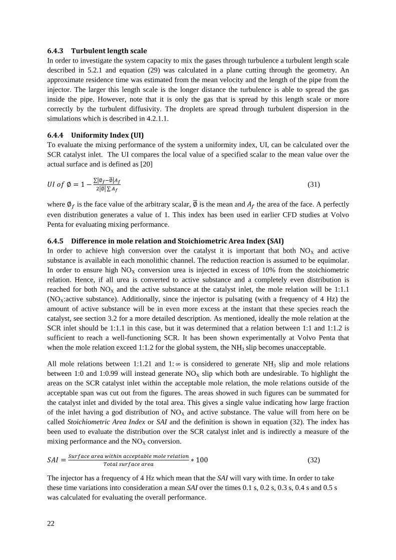
6.4.4 Uniformity Index (UI)
To evaluate the mixing performance of the system a uniformity index, UI, can be calculated over the
SCR catalyst inlet. The UI compares the local value of a specified scalar to the mean value over the
actual surface and is defined as [20]
𝑈 𝑜𝑓 ∅ ∑|∅𝑓 ∅|𝐴𝑓
|∅| ∑𝐴𝑓 (31)
where ∅𝑓 is the face value of the arbitrary scalar, ∅ is the mean and 𝑓 the area of the face. A perfectly
even distribution generates a value of 1. This index has been used in earlier CFD studies at Volvo
Penta for evaluating mixing performance.
6.4.5 Difference in mole relation and Stoichiometric Area Index (SAI)
In order to achieve high conversion over the catalyst it is important that both NOX and active
substance is available in each monolithic channel. The reduction reaction is assumed to be equimolar.
In order to ensure high NOX conversion urea is injected in excess of 10% from the stoichiometric
relation. Hence, if all urea is converted to active substance and a completely even distribution is
reached for both NOX and the active substance at the catalyst inlet, the mole relation will be 1:1.1
(NOX:active substance). Additionally, since the injector is pulsating (with a frequency of 4 Hz) the
amount of active substance will be in even more excess at the instant that these species reach the
catalyst, see section 3.2 for a more detailed description. As mentioned, ideally the mole relation at the
SCR inlet should be 1:1.1 in this case, but it was determined that a relation between 1:1 and 1:1.2 is
sufficient to reach a well-functioning SCR. It has been shown experimentally at Volvo Penta that
when the mole relation exceed 1:1.2 for the global system, the NH3 slip becomes unacceptable.
All mole relations between 1:1.21 and 1: is considered to generate NH3 slip and mole relations
between 1:0 and 1:0.99 will instead generate NOX slip which both are undesirable. To highlight the
areas on the SCR catalyst inlet within the acceptable mole relation, the mole relations outside of the
acceptable span was cut out from the figures. The areas showed in such figures can be summated for
the catalyst inlet and divided by the total area. This gives a single value indicating how large fraction
of the inlet having a god distribution of NOX and active substance. The value will from here on be
called Stoichiometric Area Index or SAI and the definition is shown in equation (32). The index has
been used to evaluate the distribution over the SCR catalyst inlet and is indirectly a measure of the
mixing performance and the NOX conversion.
𝑆𝑢𝑟𝑓𝑎 𝑒 𝑎𝑟𝑒𝑎 𝑤𝑖𝑡ℎ𝑖𝑛 𝑎 𝑒 𝑡𝑎𝑏𝑙𝑒 𝑚𝑜𝑙𝑒 𝑟𝑒𝑙𝑎𝑡𝑖𝑜𝑛
𝑜𝑡𝑎𝑙 𝑠𝑢𝑟𝑓𝑎 𝑒 𝑎𝑟𝑒𝑎 (32)
The injector has a frequency of 4 Hz which mean that the SAI will vary with time. In order to take
these time variations into consideration a mean SAI over the times 0.1 s, 0.2 s, 0.3 s, 0.4 s and 0.5 s
was calculated for evaluating the overall performance.

23
6.5 Simulation set-up
6.5.1 Case study
The conditions in the system in terms of exhaust gas flow, temperature, Adblue flow etc. will vary
with the power output from the engine. At some engine power outputs it has been proven to be very
difficult to reach high NOX conversion and will represent a worst case scenario. Therefore such power
output has been used in this study. The specifications are presented in Table 1.
Table 1: Conditions for the studied operating point
Name Exhaust gas mass flow (kg/s) Exhaust gas temperature (°C) AdBlue mass flow (g/s)
Case 1 0.281 385 0.994
6.5.2 Mixer and injector configurations
In order to investigate how the system works several system designs have been analyzed. First, static
mixers were installed in the system and both number and position of these were varied. Secondly, the
effect of the injector was analyzed by varying number and position. All studied configurations have
been given a name and these are presented in Table 2 together with their definition.
Table 2: The studied mixer and injector configurations.
Name Number
of mixers
Position (0 at
injection) [mm]
Modification to: mixer/injector
100mm 1 100 -
100,150mm 2 100, 150 -
bef&aft flex 2 100, 530 -
bef&aft inj 2 -100, 100 -
50,100mm 2 50, 100 -
50,100,150mm 3 50, 100, 150 -
100,150mm mirror 2 100, 150 Mixer at 150 mm has reversed mixer
blades
100,150mm mid inj 2 100, 150 Injection is located in the center of the
pipe
100,150mm two inj 2 100, 150 Two 4 Hz injectors injecting half amount
each of the required urea, overlapping in
time
6.5.3 Boundaries
6.5.3.1 Inlet
The inlet was specified as a mass flow rate inlet where the exhaust gas mass flow and temperature
shown in Table 1, was specified. The exhaust gas was modeled as air using mole fractions of 21%
oxygen and 79% nitrogen.
Additional boundary conditions are turbulent intensity and turbulent length scale. These were set to
10% and 10% of the pipe diameter respectively since these values have been used in earlier studies at
Volvo Penta [31]. To get an estimation of how far into the system these settings will survive, the ratio
multiplied by the average velocity at the inlet was calculated. This gave an estimated survival
distance of 0.48 m which is approximately the distance from the inlet to the spray injector. Ideally the
turbulent boundary conditions should dissipate before the spray is injected to be sure that there is no
effect on the spray droplets. Since correct turbulent boundary condition for the inlet are unknown and
since this study is focusing on investigate trends in the system rather than exact values the applied

24
boundary conditions was used in the simulations of this study. For future simulations when more exact
values are of interest it may be required to model the upstream engine device(s) to predict the
turbulence at the inlet more correctly.
6.5.3.2 Turbocharger
To investigate how the upstream turbocharger may influence the exhaust gas flow a rotational motion
was set as an inlet condition. The swirling flow was assumed to have a direction of ±20° to the main
flow direction from which a rotation speed could be calculated. The calculations can be seen in
Appendix A.
6.5.3.3 Outlet
The outlet was set to a pressure outlet with a pressure table was extracted from a plane in the full scale
geometry at the position of the outlet for the downsized geometry.
6.5.3.4 Wall
The pipe walls were specified as adiabatic and the local pipe wall temperature were set to the
temperature of the exhaust gas flow. The walls were also specified with the no-slip condition.

25
7 Sensitivity analysis In this analysis the sensitivity of the simulation results depending on turbulence model, mesh density
and the inlet velocity profile has been investigated.
7.1 Realizable k-ε vs. SST turbulence model The two RANS models was described in section 4.1.2 and 4.1.4 and are two possible turbulence
models suitable for this study. Since there is no experimental data available, the two models were
applied for the simulation configuration 100mm (see Table 2) and the results were compared to see
how the choice of turbulence model affects the solution. The results in terms of mass fractions, UI etc.
were very similar when the two turbulence models were compared. This indicates that the choice of
the turbulence model in terms of the realizable k-ε model and the SST model does not seem to affect
the final results significantly. Since the realizable k-ε model has been used in earlier studies at Volvo
Penta, this was chosen also for this study.
7.2 Analysis of mesh independence In order to analyze how the mesh influences the simulation results two different mesh densities was
investigated containing 2.2 and 3.4 million cells respectively. The mixer configuration 100mm, which
is further described in Table 2, and the realizable k-ε model was chosen for this study. This refinement
of the bulk mesh should decrease the possible existing numerical diffusion in the coarser mesh.
However, no differences could be seen in the results which indicates that the coarser mesh is sufficient
for the study.
To further analyze the mesh independence, a refinement could be done for regions where gradients
exist in the geometry. An example of a region where significant concentrations gradient exist, is the
region where the spray is injected. However, such sensitivity analysis of the mesh was not performed
but it is recommended for future studies.
7.3 Analysis of sensitivity to the upstream turbocharger Since a turbocharger is installed upstream of the mixing pipe in some installations, the effect of
applying a swirl on the inlet boundary condition was investigated. At different power outputs the swirl
rotates in different directions and since this was a general investigation, it was assumed that the flow at
the different power outputs may diverge ±20° from the axis of the flow direction. Three cases were
studied; one with no rotating motion at the inlet and two with a rotating motion corresponding to +20°
and -20° respectively.
The results showed that a rotating inlet condition will affect the result and how significant the effect
will be is dependent on how the mixers are threaded relative the rotation of the flow. Unfortunately, no
measured input data for the turbocharger was available which means that the actual inlet condition of
the exhaust gas flow could not be simulated. To be able to do this, a simulation of the turbocharger
itself has to be performed to achieve the actual flow conditions at the inlet of the mixing pipe. This
was determined to be outside the scope of this study and the effect of the turbocharger has therefore
not been taken into account in forthcoming simulations. In future work it is recommended to
investigate this effect more thoroughly so that correct inlet boundary conditions can be set for the
different power outputs. Experimental data at Volvo Penta has showed an improved NOX conversion
when the turbocharger produce a swirl. This indicates that not taking an inlet swirl into account is a
conservative way of evaluating the performance of the system. This study aims to investigate a worst
case scenario which should be the case when no swirl is generated by the turbocharger.

26
8 Results and discussion During this study many different parameters have been studied and analyzed and the understanding of
the system has gradually grown. Some of the parameters have shown to be more relevant and
important than others and are the ones presented in the report. In this section the simulation results are
presented and discussed. The section is divided into three main parts. The first is presenting a
characterization of the system and the parameters being evaluated, all described in section 6.4. The
second part is an investigation of different mixer positions and number of mixers whereas the third
part investigates the effect of position and number of injectors. The configurations investigated are
named after the mixer and injector positions where the position of the injector corresponds to zero. For
example in the 100mm configuration the mixer is positioned 100 mm downstream of the injector.
8.1 Characterization of the system In order to evaluate the modifications that will improve the SCR performance the system was first
analyzed, focusing on finding important parameters that are relevant for describing the performance.
Three different cases with zero, one (100mm) or two (100,150mm) mixers were compared. The
configurations 100mm and 100,150mm are described in Table 2.
8.1.1 Droplet size and distribution
Introducing mixers into the system is important in terms of breaking up the AdBlue droplets into
smaller ones as they hit the mixer blades. Smaller droplets require less time to evaporate which
enables a higher amount of active substance to form during the same residence time. The efficiency in
breaking up the droplets for a system with zero, one or two mixers was investigated by plotting the
distribution of the droplet diameters for the three different configurations over a plane downstream of
the injector, as is seen in Figure 12. In the case with no mixer, the plane was located 15 cm after the
injector and in the mixer cases the plane was located 5 cm from the mixer(s).
Figure 12: Droplet diameter distribution for a system without, with one or two mixers. The distribution was evaluated
in a plane 5 cm downstream of the mixer(s) and 15 cm downstream of the injector in the case without mixer(s).
There are a larger number of small droplets in the system with one and two mixers compared to a
system without mixer. This indicates that the mixers efficiently break up the droplets into smaller
ones. After the second mixer there are an even higher number of small droplets than after the first
mixer which shows that a droplet size equilibrium is not reached after one mixer.
The peak in the droplet diameter distribution is at 6 µm for two mixers and at 12 µm for one mixer
which is compared to no mixer that has the peak at 44 µm. This indicates that the second mixer is not
as efficient as the first mixer in breaking up the droplets. In order to investigate if equilibrium is
0 100 200 3000
1000
2000
3000
Droplet size [m]
Fre
qu
en
cy
No mixer
100mm
100,150mm

27
reached after the second mixer in terms of droplet diameter the distribution after a third mixer should
be studied.
8.1.2 Urea conversion
The AdBlue droplet size is an important parameter for the active substance formation. In this section
urea conversion is analyzed, which is the ratio between the total amount of formed NH3 and injected
urea during a time of 0.5 s. The conversion will be the same for HNCO since the reaction is equimolar
and because the hydrolysis HNCO is slow without any catalyst present at the present temperature
(385°C). The conversion of urea for the three studied systems is shown in Table 3.
Table 3: Urea conversion for three mixer configurations during 0.5 s.
Configuration Urea Conversion [%]
No mixer 35
1 mixer (100mm) 73
2 mixers (100,150mm) 77
The results show the same trend as the distribution of the droplet diameter. The urea conversion
increases when mixers are introduced into the system in the same way as the droplet diameter
decreases. From a poor conversion of urea in a system without mixer the conversion more than
doubles if one mixer is used. The conversion is further increased when a second mixer is introduced.
The difference between one and two mixers is not as significant as between none and one mixer, but
the conversion increases to some extent. Therefore it is concluded that the urea droplet size has a vital
impact on the formation of active substance.
8.1.3 Turbulent length scale
The turbulent length scale was calculated and evaluated in a plane cutting through the system which is
displayed in Figure 13. The results show that the case without any mixer has a larger length scale in
the middle of the pipe while it is relatively small along the wall (a). The other two systems with one
(b) and two mixers (c) instead have larger length scale along the wall and smaller in the middle of the
pipe.
Figure 13: Turbulent length scale for the system without mixer (a), one mixer (b) and two mixers (c) calculated from
the turbulent diffusivity and an approximate residence time based on the mean velocity and the pipe length from the
injector.
(a) (b)
(c)

28
Since the spray is injected from the wall, the small droplets will not penetrate so far in to the pipe but
will instead evaporate relatively fast in the area near the wall. On the other hand large droplets are able
to penetrate into the middle of the pipe but they will have a much longer evaporation time. This
behavior is substantial in the no mixer configuration but not as distinct in the cases including mixers
since the mixers enables the droplets to spread. As mentioned earlier, in the modeling turbulent
diffusion is only able to transport the gas and will not enhance the spreading of droplets. Hence, a
large turbulent length scale along the wall should be favorable which is not the case for the no mixer
configuration. However, it is not possible to determine which of the two mixer cases (one mixer and
two mixers) that is preferable.
The results also show that the largest length scale is approximately 2 cm and in the systems including
mixers it is much lower in the middle of the pipe. Since the pipe diameter is 10 cm the turbulent
diffusivity is not able spread and mix the gas over the whole cross section. The droplets will be spread
by the bulk flow and a major part of the droplets that evaporates prior to the SCR inlet will evaporate
at the end of the domain. This means that the bulk flow has a more important role when it comes to
spreading the active substance over the cross section.
The turbulent length scale is received from the steady state solution of the exhaust gases meaning that
the spray do not have to be simulated. The reason for this is that the spray in this study is weak and do
not produce any significant turbulence itself. On the other hand, when the spray produce turbulence it
is not possible to receive the turbulent length scale without simulating the spray. However, in this case
the parameter from the steady state solution could be used as an indicator for which system
modification that will generate a desirable SCR performance.
8.1.4 Uniformity Index
Earlier studies performed at Volvo Penta applied a surface uniformity index (UI) at the SCR catalyst
inlet to evaluate mixing performance of the system. The index was described in section 6.4.3 and
compares the face value of a scalar to the mean of the specific scalar and evaluates this for all cells on
the surface. A value of one indicates a perfect distribution in terms of UI. This means that a perfect
distribution of NH3 (UI=1) can be achieved even though there are no or very little NH3 at the surface.
An example of this is given in Figure 14 where UI of the NH3 mass flux is calculated at the SCR inlet
during a physical time period of 0.5 s for the case with no mixer and the case including one mixer. In
this figure these two configurations have very similar UI and should therefore have similar distribution
of NH3 mass flux over the SCR inlet. However, the distribution of NH3 mass flux over the SCR inlet at
the physical time 0.4 s (where UI of the two cases are almost identical) in Figure 15 reveals a
significant difference between the cases.

29
Figure 14: The calculated UI of the mole flux of NH3 over a physical time period of 0.5 s for the two cases; no mixer
and one mixer (100mm).
Figure 15: The distribution of NH3 mass flux over the SCR inlet at the physical time 0.4 s for the two cases; no mixer
(a) and one mixer (b).
Figure 15 clearly shows that a system without a mixer (a) do not generate an even distribution of NH3
while the distribution for a case with one mixer (b) becomes much more even. Nevertheless, the UI for
the two cases at this time are almost identical. Since the no mixer case has large areas with very low
amount of NH3 the mean value will be close to zero. It is only a small area at the top of the surface that
will diverge from the mean and thereby generating a relatively high UI. Hence, it can be concluded
that UI is not suitable for evaluating the current system. Due to this it was decided to exclude UI as a
parameter for evaluating the mixing and instead study the difference in mole relation of the involved
species at the SCR inlet.
8.1.5 Difference in mole relation and Stoichiometric Area Index (SAI)
In order to investigate the NOX conversion and the mixing performance the area of the SCR inlet
having a mole relation between 1:1 and 1:1.2 (as described in 6.4.5) was studied. The result is shown
in Figure 16 for the three studied cases. This figure shows that no mixer has the smallest area within
the acceptable range which indicates poor mixing performance and the lowest NOX conversion should
be seen in this case. In the system containing one mixer a larger area is reached and it seems to
increase even further in the case of two mixers.
0 0.1 0.2 0.3 0.4 0.50
0.2
0.4
0.6
0.8SCR inlet
Time [s]
UI of m
ass flo
w a
mm
onia
No mixer
100mm

30
Figure 16: The area that has a mole relation within the acceptable span 1:1 and 1:1.2. The three investigated
configurations are no mixer (a), one mixer (b) and two mixers (c).
The Stoichiometric Area Index in equation (32) which is also presented in 6.4.5 was calculated in
order to quantify the actual area within the specified mole relations for the three system
configurations. The results are shown in Table 4. It is confirmed that the area with a mole relation
within the specified range, increase with number of mixers. The explanation to this is that the mixers
produce turbulence by creating a swirl and thereby changing the velocity profile of the bulk flow. The
droplets are spread over the cross-section by means of the bulk flow and the mixing performance is
therefore improved when introducing a mixer. Adding a second mixer will change the velocity profile
even further and produce an even better mixing. The increase in SAI when adding mixers to the system
also depends on the decrease in droplet size and the increase in urea conversion. Hence, the system
with two mixers produces the largest area with acceptable mole relation at the SCR inlet and it also
generated the highest urea conversion. This design should therefore produce the highest NOX
conversion of these three cases.
Table 4: The calculated SAI for the three studied system configurations
Configuration SAI [%]
No mixer 7.2
One mixer (100mm) 21
Two mixers (100,150mm) 26
The SAI value is relatively low for all cases and this is caused by the pulsating injector. The mole flow
of active substance will vary considerably with time and will be reduced to almost zero between two
injections. To demonstrate the time variations for the reader, a plot of the NH3 mole flow at the SCR
inlet over a physical time period of 0.5 s is shown in Figure 17.
(a) (b)
(c) 1:1.2
1:1.16
1:1.12
1:1.08
1:1.04
1:1

31
Figure 17: The mole flow of NH3 at the SCR inlet for the three cases; no mixer, one mixer and two mixers.
The time variations due to the pulsating injector are clearly shown for all three configurations. The
two peaks correspond to the two injections taking place in 0.5 s and the mole flow is considerably
reduced between the two injections. SAI is calculated as a mean value of the area that is reached at the
times 0.1 s, 0.2 s, 0.3 s, 0.4 s and 0.5 s which means that the value will be low due to the variations in
time. It should be noted that since only five physical times are included in this value it does not take
the time variation fully into account. To get a full representation of the variations in time the SAI
should be calculated over time and then integrated. This is a recommendation for future studies which
are further discussed 10.2.
8.1.6 Important parameters for evaluating the SCR performance
In the above result section several parameters have been discussed and their significance for
understanding and estimating the SCR performance has been evaluated. It could be concluded that the
droplet size will have a strong influence on the urea conversion. Additionally, the urea conversion is a
limiting factor for the system and the NOX conversion is directly connected to this. It can also be
concluded that the SAI value is an important parameter for evaluating the actual system performance.
Hence, these parameters can be used together to evaluate the performance and quantify what system
should give the highest NOX conversion;
1. Droplets size and distribution
2. Urea conversion
3. Stoichiometric Area Index (SAI)
In the forthcoming two sections, the SCR performance was evaluated by using these parameters.
8.2 The effect of the positions of two mixers and of introducing a third
mixer to the system The 100,150mm configuration showed the most favorable results in the previous result section and
therefore the effect of the location of the two mixers on SCR performance was investigated.
Additionally, the effect of introducing a third mixer to the system was analyzed. Five new
configurations were simulated: 50,100mm; 50,100,150mm; bef&aft flex and bef&aft inj and
100,150mm mirror which are defined in Table 2. All configurations except 100,150mm mirror have
identical mixers installed. In the 100,150mm mirror case the second mixer (150 mm downstream from
the injector) was threaded in the opposite direction compared with the first mixer (100 mm
downstream from the injector). The five new configurations were compared to the three cases from the
previous section.
0 0.1 0.2 0.3 0.4 0.50
2
4
6
8x 10⁻³ Mole flow ammonia [mole/s]
Time [s]
0 0.1 0.2 0.3 0.4 0.50
2
4
6
8x 10⁻⁴ Mole flow ammonia [mole/s]
Time [s]
No mixer
100mm
100,150mm
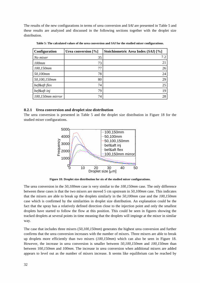
32
The results of the new configurations in terms of urea conversion and SAI are presented in Table 5 and
these results are analyzed and discussed in the following sections together with the droplet size
distribution.
Table 5: The calculated values of the urea conversion and SAI for the studied mixer configurations.
Configuration Urea conversion [%] Stoichiometric Area Index (SAI) [%]
No mixer 35 7.2
100mm 73 21
100,150mm 77 26
50,100mm 78 24
50,100,150mm 80 29
bef&aft flex 74 25
bef&aft inj 79 19
100,150mm mirror 74 28
8.2.1 Urea conversion and droplet size distribution
The urea conversion is presented in Table 5 and the droplet size distribution in Figure 18 for the
studied mixer configurations.
Figure 18: Droplet size distribution for six of the studied mixer configurations.
The urea conversion in the 50,100mm case is very similar to the 100,150mm case. The only difference
between these cases is that the two mixers are moved 5 cm upstream in 50,100mm case. This indicates
that the mixers are able to break up the droplets similarly in the 50,100mm case and the 100,150mm
case which is confirmed by the similarities in droplet size distribution. An explanation could be the
fact that the spray has a relatively defined direction close to the injection point and only the smallest
droplets have started to follow the flow at this position. This could be seen in figures showing the
tracked droplets at several points in time meaning that the droplets will impinge at the mixer in similar
way.
The case that includes three mixers (50,100,150mm) generates the highest urea conversion and further
confirms that the urea conversion increases with the number of mixers. Three mixers are able to break
up droplets more efficiently than two mixers (100,150mm) which can also be seen in Figure 18.
However, the increase in urea conversion is smaller between 50,100,150mm and 100,150mm than
between 100,150mm and 100mm. The increase in urea conversion when additional mixers are added
appears to level out as the number of mixers increase. It seems like equilibrium can be reached by
0 10 20 30 40 500
1000
2000
3000
4000
5000
Droplet size [m]
Fre
quency
100,150mm
50,100mm
50,100,150mm
bef&aft inj
bef&aft flex
100,150mm mirror

33
introducing additional mixers. At such equilibrium the urea conversion cannot be increased further by
adding mixers. In order to conclude this, the number of mixers should be increased until no difference
can be seen in urea conversion and droplet size distribution and this can be recommended for future
studies.
In the bef&aft flex case, the conversion is lowered to the level that was also found in the one mixer
case (100mm). In this system design, both mixers are placed downstream of the injector but only one
mixer is located close to the injector. This result indicates that it is important that the droplets interact
with mixers and break up early in the system since the mixer at the end of the pipe do not influence the
urea conversion. This seems reasonable since if the droplet size is reduced early, the evaporation time
will be reduced when the SCR inlet is relatively far away i.e. there is more time for evaporation and
conversion of urea. Hence, a larger number of droplets have enough time to evaporate before reaching
the inlet of the catalyst.
When one of two mixers was placed upstream of the injector (bef&aft inj) a slight increase in urea
conversion is seen compared with the 100,150mm configuration. In this case, the droplets will only
interact with one mixer. The difference from the 100mm case is that one mixer is located upstream of
the injector creating a swirl. Consequently the droplets will impinge the mixer differently and the
droplet size distribution will be different which is seen from the size distribution in Figure 18. Hence,
the droplet breakup is not only dependent on the number of mixers on a close distance downstream. It
also depends on the features of the flow field upstream of the injector, which in turn affects how and
where the droplets will impinge.
In the last configuration, one of the two mixers were threaded in different direction (100,150mm
mirror). The urea conversion is in this case similar to the conversion in the one mixer case (100mm).
However, the droplet size distribution in Figure 18 shows that there are a larger number of small
droplets in this case compared to the 100,150mm case. When the flow is forced to change direction
after the first mixer and the fact that the blades of the second mixer has the opposite direction, the
efficiency of the second mixer in terms of droplet break up is increased. This confirms the earlier
statement, that the droplet breakup is dependent on the features of the flow field upstream of the
injector. The reason for the lower urea conversion even though the mixer generates small droplets can
be explained by the residence time. It is decreased with 60% compared to residence times for the
100,150mm case which is seen in Table 11 displayed in Appendix C. The mixers are threaded in
different directions which mean that the swirl created from the mixers are canceled out generating a
relatively straight flow field and consequently a shorter residence time. This behavior is visualized in
Figure 19 where the streamlines for the 100,150mm mirror case and the 100,150mm case is compared.
This cause a more incomplete evaporation and decreased active substance formation. Hence, the
residence time is a second parameter affecting the urea conversion.

34
Figure 19: Streamlines visualizing the effect on the flow field of two mixers threaded in opposite direction (100,150mm
mirror) shown in (a) in contrast to two mixers threaded in the same direction (100,150mm) shown in (b).
8.2.2 Stoichiometric Area Index (SAI)
As mentioned, changing the position of the two mixers from 100,150mm to 50,100mm generated
similar urea conversion but the SAI value is decreased with 2%. The mixers create turbulence in terms
of a swirl that improves the mixing capacity of the system. However, turbulence is dissipative which
means that when the mixers are moved upstream the created turbulence will dissipate earlier in the
system. This could be the explanation for the decrease in SAI.
When introducing a third mixer (50,100,150mm) the SAI is increased compared to the two mixer case
(100,150mm). This confirms the conclusion drawn in the previous section that adding another mixer
will change the velocity profile even further and produce an even better mixing. Hence increasing the
number of mixers enhances the mixing capacity of the system. However, the mixers also generate a
pressure drop in the domain which will naturally increase with number of mixers. This has to be
considered when designing the system and a trade-off has to be made since a large number of mixers
may generate much better mixing but the pressure drop may be unacceptably large. The pressure drops
for all studied configurations is presented in Appendix C.
The bef&aft flex case generates a lower SAI than the 100,150mm case which indicates that it is more
favorable to place the mixers close to the injector than further downstream in the pipe. Hence, it is
important to enhance the bulk flow mixing early in the system to reach a more uniform mixture at the
inlet.
When one mixer is placed upstream of the injector (bef&aft inj) the SAI is significantly decreased
when compared to the 100,150mm case. This emphasize the discussion in the 50,100mm case, that
moving the mixers upstream also means that the created swirl from the mixers will dissipate or
decrease further upstream in the system.
In the last configuration, one of the mixers were threaded in opposite direction (100,150mm mirror)
which resulted in a SAI almost as high as for three mixers. In all other cases a more unified swirl
direction is produced since the mixers have the same mixer blade direction whereas in the 100,150mm
mirror case the flow is forced to change direction after the first mixer meaning that the flow will be
divided into several flow directions. This increases the mixing capacity of the two mixers which
(a)
(b)

35
results in a higher SAI than for the other cases with two mixers. Hence, if two mixers are to be used it
is favorable to thread them in opposite directions. The pressure drop over the mixers in the 100,150mm
configuration is the same as the pressure drop for three mixers (50,100,150mm) but it is advantageous
to use as few mixers as possible in the practical solution. The pressure drops for the configurations are
is presented in Table 12 in Appendix C.
8.3 The effect of injector position, number and injection type There are different ways in which the AdBlue can be injected. In order to investigate the differences
between different injector scenarios two different injector strategies were studied using the 100,150mm
configuration; inject the AdBlue in the middle of the pipe and use two injectors injecting one at the
time. When the spray is injected in the middle of the pipe, the spray is more evenly distributed over
the cross-sectional area which should represent a best case scenario in terms of mixing. A continuous
spray should be the best case scenario in terms of feeding the catalyst with reducing agent evenly over
time. This continuous behavior is imitated by using two injectors that inject one at the time i.e. the first
injector starts to inject at the start of the simulation and the second starts at 0.125 s. In practice this
means that active substance will be fed to the catalyst eight times per second instead of four. However,
the injection time for each pulse will be shorter. In this section the two injection strategies are studied
in comparison to the present injector (100,150mm) and the results are evaluated in terms of urea
conversion and SAI, which is shown in Table 6.
Table 6: The calculated values of the urea conversion and SAI for three different injection strategies.
Configuration Urea conversion [%] SAI [%]
100,150mm 77 26
100,150mm mid inj 61 27
100, 150mm two inj 74 30
8.3.1 Urea conversion and droplet size distribution
The urea conversion is presented in Table 6 and the droplet size distribution in Figure 20 for the
studied injector configurations.
Figure 20: Droplet size distribution for the studied injector configurations.
As seen inTable 6 the conversion of urea is decreased when the spray is injected in the center of the
pipe compared to a side injection and this may have several reasons. When the spray is injected in the
center of the pipe, a major part of the spray will follow the flow in the middle where the velocity is
high and the flow field straight and will therefore have less time to form active substance. This is
confirmed by looking at the residence time for the 100,150mm mid inj in contrast to the 100,150mm
0 5 10 15 200
1000
2000
3000
4000
5000
Droplet size [m]
Fre
quency
100,150mm
100, 150mm mid inj
100, 150mm two inj

36
case in Table 11 presented in Appendix C. Another aspect is the interaction between the droplets and
the mixer blades. Since a large number of droplets go straight through the pipe center they will be less
affected by the mixer blades and will therefore not break up to the same extent as in the case of a side
injection which is seen in Figure 20.
For the case with two injectors (100,150mm two inj) the urea conversion is lower than for the case
with one side injector (100,150mm). Each injector injects the same AdBlue mass flow as one injector
but the time duration for each pulse is shorter and the second injector is shifted in time. The injectors
are placed opposite to each other and the spray is therefore injected from two directions. As seen from
Figure 20 the 100,150mm two inj generates the same droplet distribution as 100,150mm. Since the
mixers are symmetrical and since the two injectors are positioned symmetric it seems reasonable that
the droplet size distribution is similar. The flow field used for the two simulations is also the same but
the two cases still have different urea conversion. It can be explained by the time shift in the second
injector giving half of the injected AdBlue shorter time to form active substance at the time of
evaluating the results. The urea conversion is evaluated over a time period of 0.5 and the residence
time over 0.25 s. When a single injector is used almost all droplets from an injection have passed the
SCR catalyst inlet in 0.25 s. When two injectors are used there are still droplets left in the system after
0.25 s and 0.5 s resulting in an underestimation of the residence time and the urea conversion. A better
way to be able to compare the two cases has to be determined in order to evaluate this specific case but
also future cases regarding new injection strategies.
8.3.2 Stoichiometric Area Index (SAI)
As seen from Table 6 the middle injection (100,150mm mid inj) increases the SAI compared to a side
injection. The increase is not as high as expected since the short residence time gives a lower SAI
between pulses which decreases the time averaged SAI.
The two injector case (100,150mm two inj) shows the highest SAI of all tested configuration. Since the
injectors are located opposite to each other the spreading of the droplets are enhanced resulting in a
more even distribution at the SCR inlet and a higher SAI. Furthermore, injecting the spray
alternatingly means that the catalyst is fed with active substance more evenly over time resulting in a
higher SAI over time. The effect of using two injectors would be even more substantial if a lower mass
flow is injected since the pulse duration needed to reach the same average mass flow is increased. The
two injector configuration (100,150mm two inj) is therefore recommended to investigate further to
reach a more continuous feed of active substance to the catalyst. For example an injector with a mass
flow of 3 kg/s instead of 6.3 kg/s could be studied.

37
9 Conclusions The Uniformity Index (UI) is not suitable for evaluating the SCR performance in a system
were the amount of produced active substance may be low. It is more relevant to study the
actual mole relation between the reactants.
Two assessment methods have been developed in order to evaluate the performance of the
SCR; Urea conversion and Stoichiometric Area Index (SAI). These were used to evaluate the
active substance formation and the mixing performance in the system. It has been shown that
the urea conversion is strongly dependent on the AdBlue droplet size and the residence time.
Furthermore, SAI is dependent on both the urea conversion and the mixing performed by the
bulk flow.
It was concluded that introducing mixers into the system increases both the urea conversion
and SAI which should result in higher NOX reduction. The most substantial improvement is
seen when one mixer is introduced to the system. Two and three mixers will further improve
the performance but the improvement will not be as significant.
The case with three mixers (50,100,150mm) generates the highest urea conversion and it could
be concluded that the droplets size is decreased and the urea conversion is increased as the
number of mixers are increased.
The highest SAI was reached when two injectors were used (100,150mm two inj). Since SAI
reflects the possible NOX conversion this case was considered to be the most favorable in this
study. It has potential to reach an even higher SAI if an injector with a lower mass flow is
used.

38
10 Future studies
10.1 Proposed design for further investigation of the system It has been shown that SAI was radically improved when a second mixer was laterally reversed which
indicates that breaking up of the flow is important for the mixing in the system. It is therefore
recommended in future studies to find a way to break up the flow but still retain the droplet breakup
efficiency to get a high urea conversion. A way to achieve this could be to use another type of mixer
for the second mixer position. Hence, the mixer closest to the injector could be the one used in this
study which has shown to efficiently break up droplets. The second mixer, located downstream of the
first mixer, could have another design that enhances the breakup of the flow.
It could be concluded that the urea conversion increased as the number of mixers was increased.
However, it seems like equilibrium exists where the urea conversion cannot be increased further by
introducing additional mixers. In order to conclude this, an investigation where the number of mixers
is increased until no difference can be seen in urea conversion or specifically in droplet size
distribution downstream of the mixers could be performed.
The case that included two injectors was concluded to be the most favorable configuration in this
study and this configuration is therefore recommended to investigate further. The position of the
mixers, number of mixers and type of mixer could be varied in attempt to find a more optimal design.
Additionally, the type of injector can be changed to seek a solution where the catalyst is more evenly
fed with active substance. For example an injector with a mass flow of 3 kg/s instead of 6.3 kg/s could
be studied.
In this study one operating point has been used for analyzing the performance of different design
configurations. Since the performance may be dependent on the workload it is recommended to
investigate if the trends for the different configurations in this study also can be seen for other
operating points.
In order to increase the accuracy in the simulations it is recommended to include conjugated heat
transfer and the liquid film model in future investigations. This would mean that the droplet
impingement and the droplet evaporation at the wall can be simulated more correctly giving a more
complete description of reality. The flanges on the flex pipe, where it is possible to get accumulation
of droplets are also recommended to be included. Further, the effect of the turbocharger could be
investigated using outlet data from simulations of the turbocharger at different power operating points.
10.2 Proposed improvement to evaluating methods One important aspect to further consider in future work is the urea evaporation, if the evaporation is
complete or if any droplets remain in the system at the SCR catalyst inlet. It is undesirable that
droplets enter the catalyst since it may reduce the NOX conversion and/or create solid deposits on the
catalyst surface depending on the present temperature. In this study indication of an incomplete
evaporation has been observed which emphasize the importance of quantifying it. One suggested
method is to compare the mole flow of urea in droplet form to the total injected mole flow of urea over
the time period of the simulation as displayed in equation (33). Preferably, this could be evaluated
over a plane just upstream of the SCR inlet since ideally, all urea is evaporated before entering SCR
giving a value of 0%.
𝑈𝑟𝑒𝑎 𝑖𝑛 𝑑𝑟𝑜 𝑒𝑡 𝑓𝑜𝑟𝑚 𝑜𝑡𝑎𝑙 𝑚𝑜𝑙𝑒 𝑓𝑙𝑜𝑤 𝑜𝑓 𝑢𝑟𝑒𝑎 𝑖𝑛 𝑑𝑟𝑜 𝑙𝑒𝑡 𝑓𝑜𝑟𝑚
𝑜𝑡𝑎𝑙 𝑚𝑜𝑙𝑒 𝑓𝑙𝑜𝑤 𝑜𝑓 𝑢𝑟𝑒𝑎 (33)

39
Another improvement is to take the time dependence into account in the SAI used in this study. As
already discussed, the spray is pulsating giving significant variations in the mole flow of active
substance over time. In this study, SAI were evaluated for five times (0.1 s, 0.2 s, 0.3 s, 0.4 s and 0.5 s)
and then averaged. However to fully include the time variations the index should be calculated over
the time that the simulation is run. The method for calculating SAI used in this study is unfortunately
not possible to apply for such evaluation and the method has to be further developed. However, if
additional times are taken into account in SAI the index would represent the time variations to a higher
extent and the same routine can be used for this manner.
The principle used to calculate SAI can also be used to develop new indexes describing the slip. At a
mole relation above 1:1.2 i.e. the active substance is in large excess, the risk of NH3 slip is substantial.
The index for evaluate the NH3 slip can be calculated in the same way as SAI but with a mole relation
from 1:1.21 to 1: . The same method can be used for determining the NOX slip, where the mole
relation investigated should be between 1:0 and 1:0.99.

40
11 Bibliography 1. Majewski, W.A. What are diesel emissions. 2012 2012-08 [cited 2013 21/2]; DieselNet
Technology Guide]. Available from: http://dieselnet.com/tech/emi_intro.php#intro. 2. Diesel Catalysts. 2004 2004-05 [cited 2013 21/2]; DieselNet Technology Guide]. Available
from: http://dieselnet.com/tech/cat_diesel.php. 3. R. Salib, R.K., Optimization of Ammonia Source for SCR Applications, in 2003 Mega
Conference2003. 4. Birkhold, F., et al., Analysis of the Injection of Urea-Water-Solution for Automotive SCR
DeNOx-Systems: Modeling of Two-Phase Flow and Spray/Wall-Interaction, 2006, SAE International.
5. Zhang, X., M. Romzek, and C. Morgan, 3-D Numerical Study of Mixing Characteristics of NH3 in Front of SCR, 2006, SAE International.
6. Nonroad Diesel Engines. 2010.08 [cited 2013 12/4]; Available from: http://www.dieselnet.com/standards/eu/nonroad.php.
7. Mechanism of NO reduction with non-thermal plasma. Journal of Environmental Sciences, 2005. 17(3): p. 445-447.
8. Plasma Exhaust Treatment. 2000 2000-12 [cited 2013 21/2]; DieselNet Technology Guide]. Available from: http://dieselnet.com/tech/plasma.php.
9. Yim, S.D., et al., Decomposition of Urea into NH3 for the SCR Process. Industrial & Engineering Chemistry Research, 2004. 43(16): p. 4856-4863.
10. Koebel, M., M. Elsener, and M. Kleemann, Urea-SCR: a promising technique to reduce NOx emissions from automotive diesel engines. Catalysis Today, 2000. 59(3–4): p. 335-345.
11. Roberts, G.W., Chemical Reactions and Chemical Reactors2009: John Wiley & Sons, Inc. 12. Warell, H.R.J., dikväveoxid, in Nationalencyklopedin2013. 13. Xu, L., et al., Laboratory and Engine Study of Urea-Related Deposits in Diesel Urea-SCR After-
Treatment Systems, 2007, SAE International. 14. Andreas, L., Urea Decomposition for Urea-SCR Applications, Experimental and computational
fluid dynamics studies, PhD thesis, Department of Chemical and Biological Engineering, Division of Chemical Engineering2010, Chalmers University of Technology: Gothenburg. p. 52.
15. Udo, F., Spray Systems, in Multiphase Flow Handbook2005, CRC Press. p. 8-1-8-100. 16. Lefebvre, A.H., Atomization and Sprays. Combustion: An International Series, ed. N.
Chigier1989, United States of America: Hemisphere Publishing Corporation. 17. Crowe, C.T., Particle-Fluid Interaction, in Multiphase Flows with Droplets and Particles,
Second Edition2011, CRC Press. p. 57-117. 18. Chen, C., et al., Detailed Modeling of Liquid Fuel Sprays in One-Dimensional Gas Flow
Simulation, 2004, SAE International. 19. Andersson, B., Andersson, R., Håkansson, L., Mortensen, M., Sudiyo, R. and van Wachem, B.,
Computational Fluid Dynamics for Engineers, Cambridge University Press, 2012. 20. STAR CCM+ v.8.02.008 Theory Guide, 2013. 21. Crowe, C.T., Properties of Dispersed Phase Flows, in Multiphase Flows with Droplets and
Particles, Second Edition2011, CRC Press. p. 17-38. 22. Crowe, C.T., Droplet-Particle Cloud Equations, in Multiphase Flows with Droplets and
Particles, Second Edition2011, CRC Press. p. 235-258. 23. turboaggregat, in Nationalencyklopedin. 24. Hall, S.L.D.C.A., Fluid Mechanics and Thermodynamics of Turbomachinery. 6th ed2010,
Oxford: Butterworth-Heinmann. 25. Coulson, J.M., et al., Coulson and Richardson's Chemical Engineering Volume 1 - Fluid Flow,
Heat Transfer and Mass Transfer (6th Edition), Elsevier. 26. Webster, P.J.W.R.a.D.R., Turbulent Diffusion, in Environmental Fluid Mechanics: Theories and
Applications2002, American Society of Civil Engineers. p. 7-45.

41
27. Bourne, J.B.a.J.R., Turbulent Mixing and Chemical Reactions1999, Chichester, England: John Wiley & Sons Ltd.
28. Andersson, B., Private communication, 2013. 29. Rajadurai, S., Improved NOx Reduction Using Wiremesh Thermolysis Mixer in Urea SCR
System, 2008, SAE International. 30. Tsinoglou, D. and G. Koltsakis, Modelling of the selective catalytic NOx reduction in diesel
exhaust including ammonia storage. Proceedings of the Institution of Mechanical Engineers, Part D: Journal of Automobile Engineering, 2007. 221(1): p. 117-133.
31. Edman, J., A urea spray simulation study of a Volvo Penta C15 muffler and the R22 system, 2012.
32. Tae Joong Wang, S.W.B., and Seung Yeol Lee, Experimental Investigation on Evaporation of Urea-Water-Solution Droplet for SCR Applications. AIChE, 2009. 55(12): p. 3267-3276.
33. Hellsten, S.-E.M.a.G., DATA OCH DIAGRAM. 7th ed2008, Stockholm: Liber AB. 34. Efstathios, M. and C. Clayton, Basic Concepts and Definitions, in Multiphase Flow
Handbook2005, CRC Press. p. 1-1-1-79.

42
A Appendix – Calculation of rpm for the swirling flow Velocity is equal to the volume flow rate divided by the cross section area of the pipe.
𝑞
𝐴
𝑚 𝑠
𝑚2
To get velocity from a mass flow the density is needed
𝑚
𝜌
𝐴
Following figure illustrates the velocity component for a 20° deviation from the flow direction. 𝑥 is
the velocity in the flow direction and 𝑠 represents the velocity component for a 20° deviation.
If 𝑥 is known, 𝑠 can be calculated through the relation below.
𝑣
𝑣 𝑠 𝑥
The pipe diameter is 0.104 m which gives a circumference of 0.3267 m. The rotational speed of the
flow in rpm corresponding to the velocity 𝑠 can be calculated by following equation.
𝑟 𝑚 𝑣
For an operating point with an exhaust mass flow rate of 0.26 kg /s and a mean density in the inlet of
0.5937 kg/m3 the velocity in the flow direction becomes
𝑥
(
2)2
𝑚
This will give a 𝑠 of
𝑠 𝑥 𝑚
and finally the rpm is calculated.
𝑟 𝑚 𝑣
4 44
4
vx
20° vs

43
B Appendix – Calculation of droplet evaporation, Stoke’s
number and thermal response time
Droplet evaporation time and length The D
2-law presented in (*) was used to calculate an approximation of the evaporation time. The
maximum and minimum size of the injected droplets is 300 μm and 2 μm respectively.
𝜆𝑡 (*)
To calculate the evaporation time, the evaporation rate coefficient λ is needed and the experimental
data from [32] was used to calculate this. Three data points at 673 K were taken from Figure 14 in [32]
and these are listed in Table 7.
Table 7: Experimental data from [32].
Initial diameter (D0) of Urea-Water-Solution Droplet [mm] Rate Coefficient (λ) [mm2/s]
0.07 0.036
1 0.039
1.34 0.044
A linear regression was constructed from these three points and is given in equation (**).
𝜆 (**)
By using these two equations and defining D=0, an approximate evaporation time for the largest and
the smallest droplets could be calculated. The average velocity in the domain is 30 m/s (for a
temperature of 658 K) and from this the typical length needed for evaporating the droplets can be
calculated. The results are presented in Table 8.
Table 8: Calculated values of the evaporation time for the largest and the smallest simulated droplets.
Initial diameter (D0) [μm] Evaporation time (t) [s] Needed length [m]
300 2.45 73.5
2 1.14*10-4
0.00342
Hence, the evaporation time spans from less than ms up to a few seconds which emphasize the
significance of the droplet size and residence time. It can be concluded that the largest droplets will
not have enough time for evaporation since these will need approximately 70 m. This means that it is
not possible to reach full conversion of urea if the droplet size is not reduced and there will be urea left
that enters the SCR catalyst.
Stoke’s number To get an idea of how well the droplet will follow the flow and adjust to changes in the flow the
Stoke’s number was calculated for the largest and the smallest simulated droplets. The derived
equations in this section comes from [19]. The Stoke´s number for a droplet is defined as
𝑡 𝜏
𝜏𝑓
where 𝑑 is droplet response time and 𝑓 is the characteristic time scale for the flow. The droplet
response time for non-Stoke’s flow may be calculated by
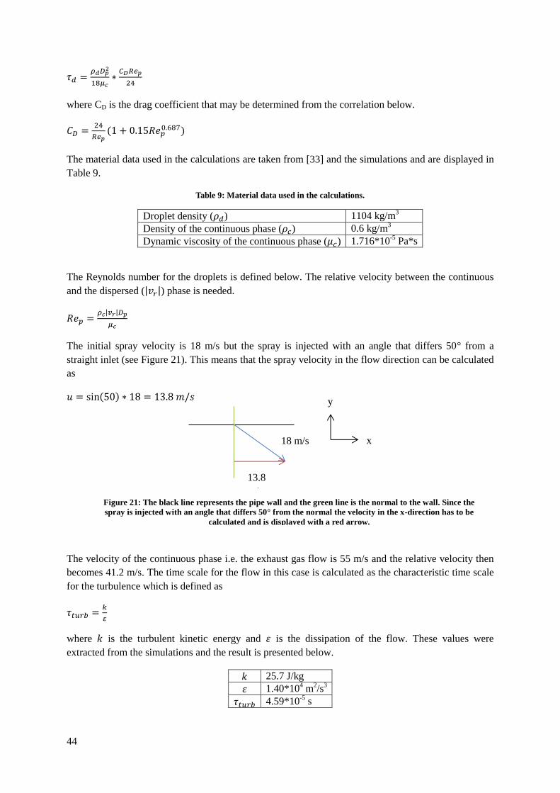
44
𝑑 𝜌 𝐷𝑝
2
𝜇𝑐
𝑒𝑝
4
where CD is the drag coefficient that may be determined from the correlation below.
𝐶𝐷 4
𝑒𝑝 𝑒
The material data used in the calculations are taken from [33] and the simulations and are displayed in
Table 9.
Table 9: Material data used in the calculations.
Droplet density ( 𝑑) 1104 kg/m3
Density of the continuous phase ( ) 0.6 kg/m3
Dynamic viscosity of the continuous phase ( ) 1.716*10-5
Pa*s
The Reynolds number for the droplets is defined below. The relative velocity between the continuous
and the dispersed (| 𝑟|) phase is needed.
𝑒 𝜌𝑐|𝑣 |𝐷𝑝
𝜇𝑐
The initial spray velocity is 18 m/s but the spray is injected with an angle that differs 50° from a
straight inlet (see Figure 21). This means that the spray velocity in the flow direction can be calculated
as
𝑢 n 𝑚
The velocity of the continuous phase i.e. the exhaust gas flow is 55 m/s and the relative velocity then
becomes 41.2 m/s. The time scale for the flow in this case is calculated as the characteristic time scale
for the turbulence which is defined as
𝑡𝑢𝑟𝑏 𝑘
𝜀
where is the turbulent kinetic energy and 𝜀 is the dissipation of the flow. These values were
extracted from the simulations and the result is presented below.
25.7 J/kg
𝜀 1.40*104 m
2/s
3
𝑡𝑢𝑟𝑏 4.59*10-5
s
18 m/s
13.8
m/s
y
x
y
Figure 21: The black line represents the pipe wall and the green line is the normal to the wall. Since the
spray is injected with an angle that differs 50° from the normal the velocity in the x-direction has to be
calculated and is displayed with a red arrow.

45
For a droplet diameter of 300 μm the Stoke’s number was calculated to approximately 1800 i.e. St>>1.
This means that the largest droplets do not follow the flow initially. For a droplet diameter of 2 μm the
Stoke’s number was calculated to approximately 0,1 i.e. St≈1. The smallest droplets will follow the
flow to some extent from the moment they are injected. Hence, the flow field is an important factor for
the spreading of the droplets and it should be preferable to have a turbulent flow that can allocate the
droplets.
Thermal response time The thermal response time is the time it takes for a droplet to respond to a change in temperature of the
continuous phase. If it is assumed that temperature is uniform throughout the droplet and that
radioactive effect is negligible, the equation for the particle temperature can be defined as
𝑑
𝑑𝑡
𝑢𝑝
𝑘𝑐
𝜌𝑝 𝐷𝑝2 𝑑
where 𝑑 is the specific heat of the droplet material and is the thermal conductivity of the
continuous phase. The temperatures and 𝑑 is the temperature of the continuous phase and the
droplet respectively [34]. The Nusselt number for the droplets can be calculated from the correlation
below
𝑢 𝑒
𝑟
The Prandtl number is defined as
𝑟 𝑝𝜇𝑐
𝑘𝑐
where is the specific heat of the continuous phase [20]. The thermal equation including the thermal
response time ( ) for the particle can be written as [34]
𝑑
𝑑𝑡
𝜏𝑇 𝑑
Hence, the thermal response time for the droplet may be calculated through following equation.
𝜌𝑝 𝐷𝑝
2
𝑘𝑐 + 𝑒𝑝 2
𝑟
The droplet material is a urea-water solution consisting of urea (32.5wt %) and water (67.5wt %) and
has an initial temperature of 30°. However, it is assumed to have the same material properties as water
in these calculations. The continuous phase is simulated as air and the temperature varies with the
power output from the engine. In these calculations it is assumed that the exhaust gases have a
temperature of 400°. The material data that is used in the calculations was taken from [33] and the
simulations and are displayed in Table 10.
Table 10: Material data used in the calculations.
Droplet density ( at 30°) 995.7 kg/m3
Specific heat of the droplets ( 𝑑 at 30°) 4175 J/kg*K
Specific heat of the continuous phase ( at 400°) 1070 J/kg*K
Thermal conductivity of the continuous phase ( at 400°) 0.0515 W/m*K
Dynamic viscosity of the continuous phase 1.716*10-5
Pa*s

46
For a droplet diameter of 300 μm the was calculated to approximately 0.1 s and for a droplet
diameter of 2 μm it was calculated to approximately 2*10-5
s.

47
C Appendix – Residence time and mixer pressure drop
Table 11: The mean residence time for a droplet from the injection point to the SCR inlet for all studied cases.
Configuration Residence time [s]
No mixer 0.002
100mm 0.025
100,150mm 0.026
50,100,150mm 0.041
50,100mm 0.031
bef&aft inj 0.030
100,150mm mirror 0.010
100,150mm mid inj 0.010
100,150mm two inj 0.013
Table 12: Pressure drop over the mixer(s) for all studied configurations.
Configuration Pressure drop [Pa]
100mm 1700
100,150mm 2600
50,100mm 2600
50,100,150mm 3700
bef&aft flex 3200
bef&aft inj 2900
100,150mm mirror 3700