a cell-based row-structure layout decomposer for triple patterning lithography hsi-an chien,...

A Cell-Based Row-Structure Layout Decomposer for Triple Patterning Lithography

Hsi-An Chien, Szu-Yuan Han, Ye-Hong Chen, and Ting-Chi Wang

Department of Computer ScienceNational Tsing Hua University

TAIWAN

Outline Introductions

Multiple patterning lithographyMotivation

ProblemTPL layout decomposition

ApproachGraph modelSpeed-up

Experimental Results Conclusion

2

3

Multiple Patterning Lithography (MPL) MPL uses multiple litho-etch (LE) steps to enhance feature

printability

Double Patterning Lithograph (DPL) 20nm/16nm LELE Two masks

Triple Patterning Lithograph (TPL) 10nm or beyond High density layer (M1 layer) LELELE Three masks Mask 1

Mask 2

Mask 3

Coloring Conflict

stitch

TPLDPL

a

b

a

b

a

b

Mask 1

Mask 2

4

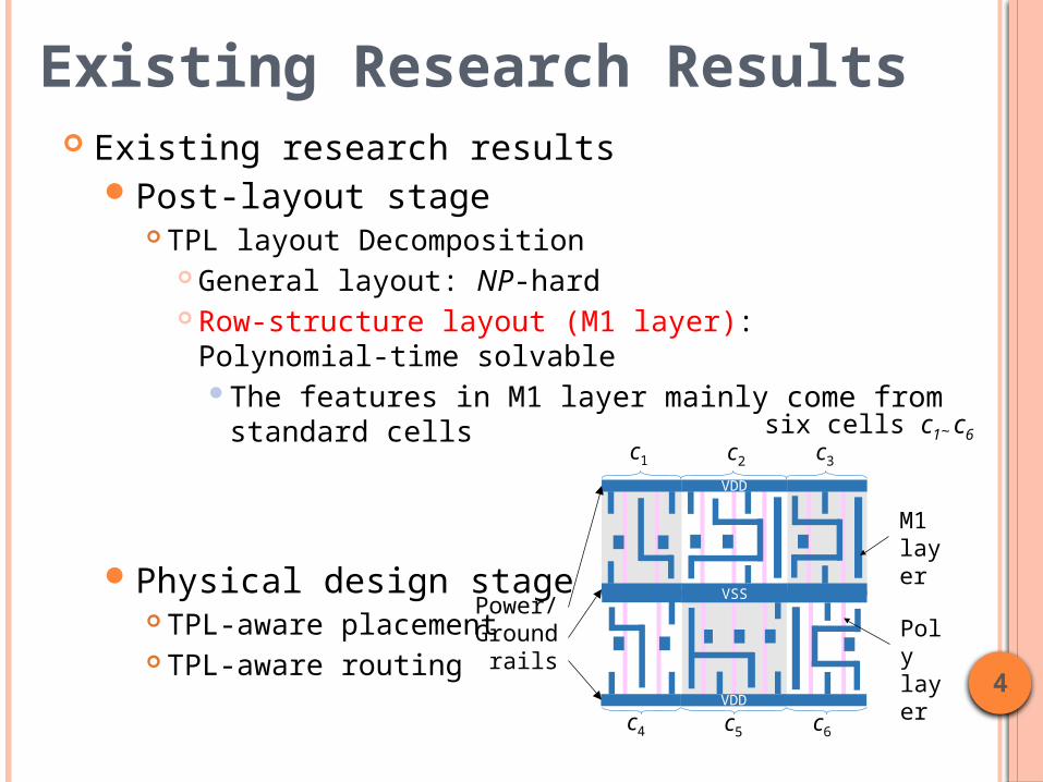
Existing Research Results Existing research results

Post-layout stage TPL layout Decomposition

General layout: NP-hard Row-structure layout (M1 layer): Polynomial-time solvable

The features in M1 layer mainly come from standard cells

Physical design stage TPL-aware placement TPL-aware routing

M1 layer

Poly layer

Power/Ground

rails

c1 c2 c3

c4 c5 c6

VDD

VSS

VDD

six cells c1~ c6

5

Motivation TPL layout decomposition for row-structure layout

Decomposable layout Polynomial-time solvable*

Decomposition solution with the minimal stitches Indecomposable layout

No decomposition solution Hard to help designers further modify the layout

Resolve coloring conflicts Decomposition solution with the minimal total cost

Coloring conflicts Stitches

*H. Tian, H. Zhang, Q. Ma, Z. Xiao, and M. D. F. Wong, “A polynomial time triple patterning algorithm for cell based row-structure layout”, in ICCAD, 2012.

6

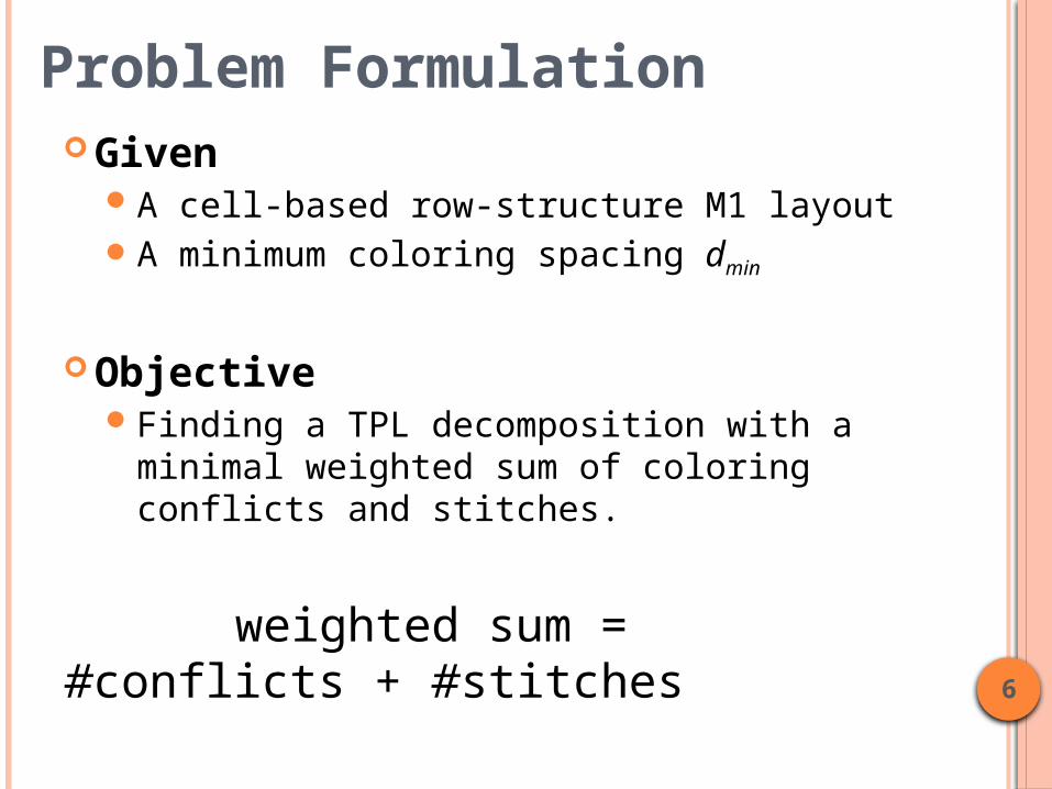
Problem Formulation Given

A cell-based row-structure M1 layoutA minimum coloring spacing dmin

ObjectiveFinding a TPL decomposition with a minimal weighted

sum of coloring conflicts and stitches.

weighted sum = #conflicts + #stitches

7

Conflict graph An undirected graph. Node: polygon in the given layout. Edge: the distance between two

corresponding polygons is less than dmin

Cutting line A vertical line aligned with the left

boundary of at least one polygon Cutting line set

A set of polygons intersecting with the corresponding cutting line

Conflict graph

a

b

c

d

l1 l2 l3

Cutting lines

s1

s2

s3{a,

b}{b, c}

{d}

Cutting line sets

Review of A Layout Decomposer*

*H. Tian, H. Zhang, Q. Ma, Z. Xiao, and M. D. F. Wong, “A polynomial time triple patterning algorithm for cell based row-structure layout”, in ICCAD, 2012.

8

Solution Graph (SG): directed graph Each node records a coloring solution of all the polygons in a

cutting line set All the possible coloring solutions are enumerated

a

b

c

ds1

s2

s3{a,

b}{b, c}

{d}

l1 l2 l3

Graph Model (1/3)

1,21,3

1,1

3,3

1

2

33,3

{d}

………… 2,1

1,21,3

1,1

2,1 ……v3

……

{a, b}

{b, c}

v1 v2

Solution Graph

9

Weight on a node#conflicts induced by polygons in the which is a subset of

cutting line set

a

b

c

ds1

s2

s3{a,

b}{b, c}

{d}

l1 l2 l3

1,21,3

1,1

3,3

1

2

33,3

{d}

………… 2,1

1,21,3

1,1

2,1

1

1

……v3

……

{a, b}

{b, c}

v1 v2

Solution Graph

Graph Model (2/3)

10

Weight on a node#conflicts induced by polygons in the which is a subset of

cutting line set Weight on an edge

#conflicts induced between all pairs of polygons (p, q), p and q

a

b

c

ds1

s2

s3{a,

b}{b, c}

{d}

l1 l2 l3

Graph Model (2/3)

1

1,21,3

1,1

3,3

1

2

33,3

{d}

………… 2,1

1,21,3

1,1

2,1

1

1

1

……

21

11

2

1

1

v3

……

{a, b}

{b, c}

v1 v2

Solution Graph

11

Graph Model (3/3) Differences

Invalid coloring solution Node Edge

Conflict cost

Lemma 1 Each possible decomposition of the layout P without stitch

insertion corresponds to a path in the SG of P Lemma 2

The TPL layout decomposition problem without stitch insertion for P can be optimally solved by finding a least-cost path in the SG of P

1

1,21,3

1,1

3,3

1

2

33,3

………… 2,1

1,21,3

1,1

2,1

1

1

1

1

1

……

21

11

2

1

1

v3……

v1 v2

12

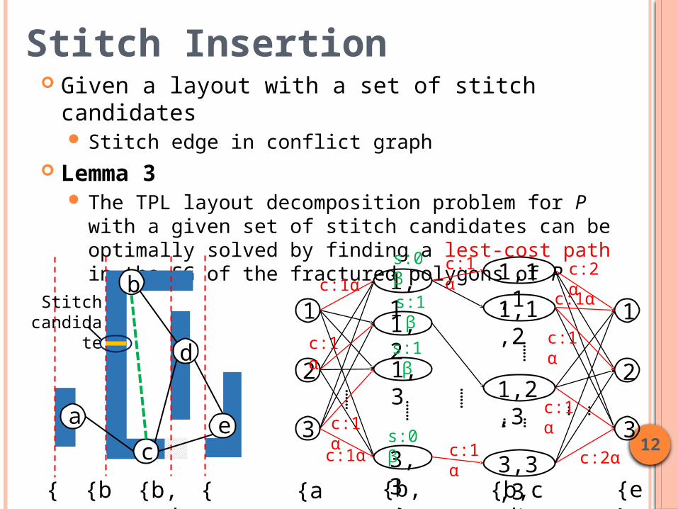
Stitch Insertion Given a layout with a set of stitch candidates

Stitch edge in conflict graph Lemma 3

The TPL layout decomposition problem for P with a given set of stitch candidates can be optimally solved by finding a lest-cost path in the SG of the fractured polygons of P

{b,c}

{a}

{b,c,d}

{e}

b

ec

d

a

Stitch candidate

1,11

2

3

1

2

1,2

1,3

3,3 3,3,3

1,1,1

1,1,2

1,2,3

{b,c}{a} {b,c,d} {e}

…… ……

…… ……

s:1β

s:0 β

c:1α

c:1α

c:1α

c:1α

c:2α

c:1α

c:1α

c:1α

c:2α

c:1α

c:1α

s:1 β

s:0β

……

……

3

13

Table Look-up (1/2) Speed-up

Store the SG for each cell in the cell library Copy the SG from the table for each cell instance Conflicts between two adjacent cells ?

Boundary conflicting polygon set (BCP)

ad

c

b e

f

dmin dminc1 c2

BCP of c1 and c2

de

Conflict graph of the BCP

14

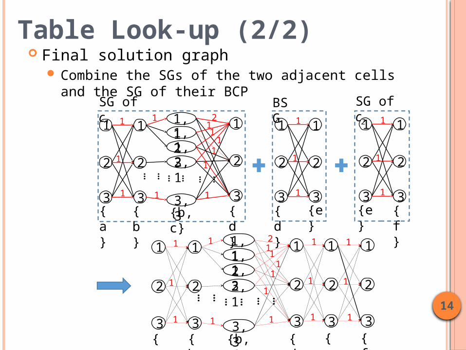
Table Look-up (2/2) Final solution graph

Combine the SGs of the two adjacent cells and the SG of their BCP

BSG

{d}

1

2

3{e}

1

2

31

1

1

SG of c2

{e}

1

2

3{f}

1

2

31

1

1

SG of c1

1

2

3

1

2

31

1

11,21,32,1

1,1

3,3{d}

1

2

3

………… ……

1

1 1

21

1

11

{a} {b} {b,c}

1

{a}

1

2

3{b}

1

2

31

1

1

{b,c}

1,21,32,1

1,1

3,3{d}

1

2

3

………… ……

1

1 1

21

1

1

1

{e}

1

2

3{f}

1

2

31

1

1

1

1

1

1

15

Too many nodes and edges Graph size Performance

Drawback of Solution Graph

#nodes = 27#edges = 0

16

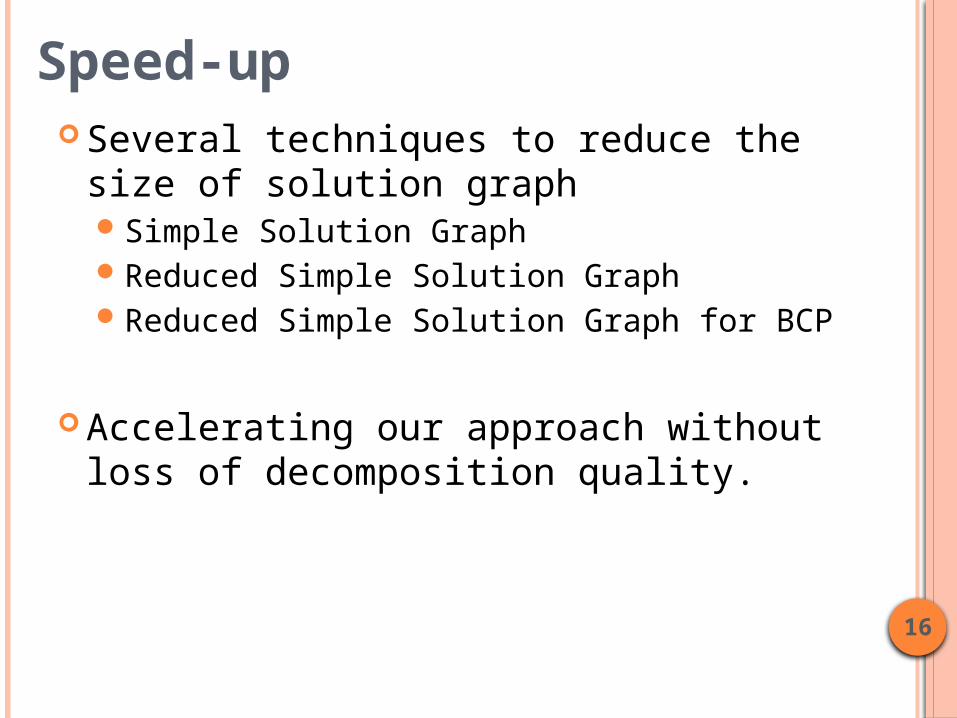
Speed-up Several techniques to reduce the size of solution

graphSimple Solution GraphReduced Simple Solution GraphReduced Simple Solution Graph for BCP

Accelerating our approach without loss of decomposition quality.

17

Observation Let Pci be the set of polygons in the M1 layer of a cell ci

The left boundary set (LBS) LBSci

Right boundary set (RBS) RBSci

Other polygons (OP) OPci = Pci \ ( LBSci RBSci )

a bc

dmindmin

{a,b}LBS

{b}RBS

{c}OP

18

Simple Solution Graph The simple solution graph of Pci is defined as a solution

graph for LBSci RBSci

An edge connecting from a node of LBSci to a node of RBSci

An optimal coloring solution of OPci and the corresponding cost

a bc

dmindmin

{a,b}LBS

{b}RBS

{c}OP

1,21,3

1,1

2,1

3,1

2,2

3,2

2,3

3,3

321

An edge records an optimal coloring solution and the corresponding cost for the OP = {c}

{a,b} {b} 12 9

({2} , 0)coloring solution

corresponding cost ({3} , 0)

v1

v2

#nodes = 39 #edges = 36

19

Reduced Simple Solution Graph (1/5) If the LBS has n polygons and the RBS has m polygons, the

number of the edges between them could be up to 3m+n

32 33


20

Reduced Simple Solution Graph (2/5) To reduce the number of the edges

Dummy LBS (DLBS) for the LBSDummy RBS (DRBS) for the RBS

The DLBS and DRBS are two subsets of LBS and RBS, respectively

Each polygon in the DLBS (DRBS) might cause a coloring conflict with at least a polygon in RBS (LBS) or OP

21

Reduced Simple Solution Graph (3/5)

{a,b}LBS

1,1

3,3

1,2

…RBS

{e,f,g}

1,1,11,1,21,1,31,2,1

3,3,3

…

DLBS{a}

2

1

3

DRBS{e,f}

1,2

1,1

…

3,3

…

……


Scenario 1: DLBS ⊂ LBS and DRBS ⊂ RBS, where both the DLBS and DRBS are not empty sets

Both the DLBS and the DRBS are added into the graph


22


1,1

3,3

1,2

…

1,1

3,3

1,2

…1,1

3,3

1,2

…

1,1

3,3

1,2…

1,1,2

1,1,3

1,2,1

3,3,3

1,1,1

{a,b}LBS RBSDRBS

{e,f,g}{e,f}{a,b} {e,f}DRBSDLBS

=

… …


Scenario 2: DLBS = LBS or DRBS = RBS, where both the DLBS and DRBS are not empty sets

Do not create the DLBS or the DRBS



23

1,2

1,1

…3,3

{a,b}LBS

1,1,11,1,21,1,31,2,1…

RBS

3,3,3{e,f,g}

No conflict with OP or RBS

pseudo node1,1

3,3

1,2

…

DRBS{e,f}

… ……


Scenario 3: DLBS and/or DRBS is an empty set A pseudo node with weight of 0 is created for the DLBS

(DRBS), if DLBS (DRBS) is an empty set

{ }DLBS


24

Reduced Simple Solution Graph for BCP

1,3

1,1

2,1

{a,b} LBSc2

……

1,2

3,3>dmin 3

2

1

{b’}RBSc1

pseudo node

{ }DRBSc1

{ } DLBSc2


#nodes = 13 #edges = 12 BCP of c1 and c2

As we redesign the solution graph to be the reduced simple solution graph for a cell, the original solution graph for a BCP cannot be directly used to combine with a reduced simple solution graph.

25

Overall Approach Given a cell library and a set of stitch candidates for

each cellOff-line build a look-up table

Reduced simple solution graph Each cell type The BCP of each cell pair

For each row Construct solution graph Find a least-cost path

Simultaneously solving the TPL layout decomposition problem for each row

26

Experimental Results Workstation with 2.0 GHz Intel Xeon CPU and 96 GB memory

Compare with two state-of-art TPL decomposers

Decomposer-A

Decomposer-B

The stitch candidates*

*J. Kuang and E. F. Y. Young, “An efficient layout decomposition approach for triple patterning lithography,” in DAC, 2013.

B. Yu, Y.-H. Lin, G. Luk-Pat, D. Ding, K. Lucas, and D. Z. Pan, “A high-performance triple patterning layout decomposer with balanced density”, in ICCAD, 2013.

H. Tian, H. Zhang, Q. Ma, Z. Xiao, and M. D. F. Wong, “A polynomial time triple patterning algorithm for cell based row-structure layout”, in ICCAD, 2012.

27

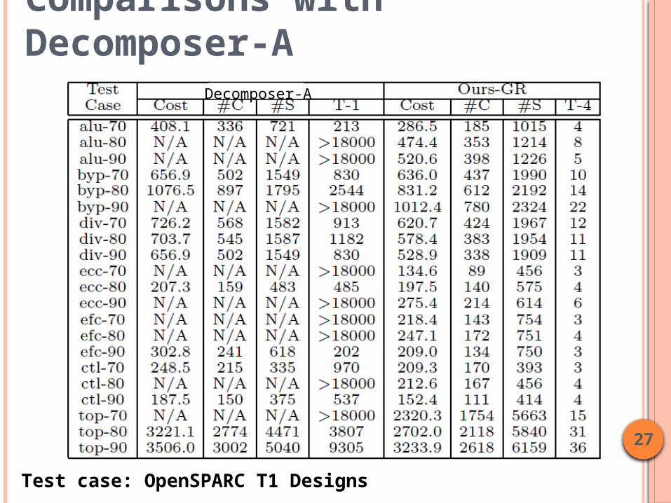
Comparisons with Decomposer-ADecomposer-A

Test case: OpenSPARC T1 Designs

28#nodes #edges T-1(s) T-2(s) T-4(s)

0

0.2

0.4

0.6

0.8

1

1.2

1 1 1 1 1

0.06

0.23 0.2 0.2 0.24

Ours Ours-GR

Ratio

Comparisons of Our Approaches

Test case: OpenSPARC T1 Designs

29

Comparisons with Decomposer-A&-B

Decomposer-B Decomposer-A

Test case: ISCAS-85&89 circuits

30

We extend an existing approach to optimally solve a row-structure TPL layout decomposition problem

Several methods to substantially reduce the graph size and hence to speed up the extended approach are also presented

The experimental results show that our approach is not only efficient but also effective

Conclusion

a cell-based row-structure layout decomposer for triple patterning lithography hsi-an chien,...

Documents

b mask

b c d s1s1 s2s2 s3s3

b c d l1l1 l2l2 l3l3

given layout

solution graph sg

cells c

undirected graph

decomposition solution