a catalogue of sturm-liouville di erential equationsmath.niu.edu/sl2/papers/birk0.pdf · a...
TRANSCRIPT
A Catalogue of Sturm-Liouvilledifferential equations
W.N. Everitt
Dedicated to all scientists who, down the long years,
have contributed to Sturm-Liouville theory.
Abstract. The idea for this catalogue follows from the conference entitled:
Bicentenaire de Charles Francois Sturm
held at the University of Geneva, Switzerland from 15 to 19 September 2003.One of the main interests for this meeting involved the historical developmentof the theory of Sturm-Liouville differential equations. This theory began withthe original work of Sturm from 1829 to 1836 and was then followed by theshort but significant joint paper of Sturm and Liouville in 1837, on second-order linear ordinary differential equations with an eigenvalue parameter.
The details of the early development of Sturm-Liouville theory, fromthe beginnings about 1830, are given in a historical survey paper of JesperLutzen (1984), in which paper a complete set of references may be found tothe relevant work of both Sturm and Liouville.
The catalogue commences with sections devoted to a brief summaryof Sturm-Liouville theory including some details of differential expressionsand equations, Hilbert function spaces, differential operators, classification ofinterval endpoints, boundary condition functions and the Liouville transform.
There follows a collection of more than 50 examples of Sturm-Liouvilledifferential equations; many of these examples are connected with well-knownspecial functions, and with problems in mathematical physics and appliedmathematics.
For most of these examples the interval endpoints are classified withinthe relevant Hilbert function space, and boundary condition functions aregiven to determine the domains of the relevant differential operators. In manycases the spectra of these operators are given.
The author is indebted to many colleagues who have responded to re-quests for examples and who checked successive drafts of the catalogue.
Received by the editors 20 February 2004.1991 Mathematics Subject Classification. Primary; 34B24, 34B20, 34B30: Secondary; 34L05,
34A30, 34A25.
Key words and phrases. Sturm-Liouville differential equations; special functions; spectral theory.
2 W.N. Everitt
Contents
1. Introduction 42. Notations 53. Sturm-Liouville differential expressions and equations 54. Operator theory 65. Endpoint classification 76. Endpoint boundary condition functions 87. The Liouville transformation 98. Fourier equation 109. Hypergeometric equation 1110. Kummer equation 1311. Bessel equation 1412. Bessel equation: Liouville form 1513. Bessel equation: form 1 1614. Bessel equation: form 2 1615. Bessel equation: form 3 1716. Bessel equation: form 4 1717. Bessel equation: modified form 1818. Airy equation 1919. Legendre equation 1920. Legendre equation: associated form 2021. Hermite equation 2122. Hermite equation: Liouville form 2123. Jacobi equation 2124. Jacobi equation: Liouville form 2325. Jacobi function equation 2426. Jacobi function equation: Liouville form 2527. Laguerre equation 2628. Laguerre equation: Liouville form 2629. Heun equation 2730. Whittaker equation 2831. Lame equation 2932. Mathieu equation 3033. Bailey equation 3134. Behnke-Goerisch equation 3135. Boyd equation 3236. Boyd equation: regularized 3237. Dunford-Schwartz equation 3338. Dunford-Schwartz equation: modified 3439. Hydrogen atom equation 3539.1. Results for form 1 3539.2. Results for form 2 3640. Algebro-geometric equations 37
Sturm-Liouville differential equations 3
40.1. Algebro-geometric form 1 3840.2. Algebro-geometric form 2 3840.3. Algebro-geometric form 3 3940.4. Algebro-geometric form 4 4041. Bargmann potentials 4242. Halvorsen equation 4443. Jorgens equation 4544. Rellich equation 4545. Laplace tidal wave equation 4646. Latzko equation 4747. Littlewood-McLeod equation 4748. Lohner equation 4849. Pryce-Marletta equation 4850. Meissner equation 4951. Morse equation 5052. Morse rotation equation 5053. Brusencev/Rofe-Beketov equations 5153.1. Example 1 5153.2. Example 2 5154. Slavyanov equations 5254.1. Example 1 5254.2. Example 2 5254.3. Example 3 5255. Fuel cell equation 5356. Shaw equation 5357. Plum equation 5458. Sears-Titchmarsh equation 5459. Zettl equation 5560. Remarks 5661. Acknowledgments 5662. The future 56References 57

4 W.N. Everitt
1. Introduction
The idea for this paper follows from the conference entitled:
Bicentenaire de Charles Francois Sturm
held at the University of Geneva, Switzerland from 15 to 19 September 2003. Oneof the main interests for this meeting involved the development of the theory ofSturm-Liouville differential equations. This theory began with the original workof Sturm from 1829 to 1836 and then followed by the short but significant jointpaper of Sturm and Liouville in 1837, on second-order linear ordinary differentialequations with an eigenvalue parameter. Details for the 1837 paper is given asreference [56] in this paper; for a complete set of historical references see thehistorical survey paper [59] of Lutzen.
This present catalogue of examples of Sturm-Liouville differential equationsis based on four main sources:
1. The list of 32 examples prepared by Bailey, Everitt and Zettl in the year2001 for the final version of the computer program SLEIGN2; this list isto be found within the LaTeX file xamples.tex contained in the packageassociated with the publication [11, Data base file xamples.tex]; all these32 examples are contained within this catalogue.
2. A selection from the set of 59 examples prepared by Pryce and publishedin 1993 in the text [69, Appendix B.2]; see also [70].
3. A selection from the set of 217 examples prepared by Pruess, Fulton andXie in the report [68].
4. A selection drawn up from a general appeal, made in October 2003, forexamples but with the request relayed in the following terms; examples tobe included should satisfy one or more of the following criteria:(i) The solutions of the differential equation are given explicitly in terms
of special functions; see for example Abramowitz and Stegun [1], theErdelyi at al Bateman volumes [27], the recent text of Slavyanov andLay [77] and the earlier text of Bell [16].
(ii) Examples with special connections to applied mathematics and math-ematical physics.
(iii) Examples with special connections to numerical analysis; see the workof Zettl [81] and [82].
The overall aim was to be content with about 50 examples, as now to be seenin the list given below.
The naming of these examples of Sturm-Liouville differential equations issomewhat arbitrary; where named special functions are concerned the chosen nameis clear; in certain other cases the name has been chosen to reflect one or more ofthe authors concerned.

Sturm-Liouville differential equations 5
2. Notations
The real and complex fields are represented by R and C respectively; a generalinterval of R is represented by I; compact and open intervals of R are representedby [a, b] and (a, b) respectively. The prime symbol ′ denotes classical differentiationon the real line R.
Lebesgue integration on R is denoted by L, and L1(I) denotes the Lebesgueintegration space of complex-valued functions defined on the interval I. The localintegration space L1
loc(I) is the set of all complex-valued functions on I which areLebesgue integrable on all compact sub-intervals [a, b] ⊆ I; if I is compact thenL1(I) ≡ L1
loc(I).Absolute continuity, with respect to Lebesgue measure, is denoted by AC; the
space of all complex-valued functions defined on I which are absolutely continuouson all compact sub-intervals of I, is denoted by ACloc(I).
A weight function w on I is a Lebesgue measurable function w : I → R
satisfying w(x) > 0 for almost all x ∈ I.Given an interval I and a weight function w the space L2(I;w) is defined as
the set of all complex-valued, Lebesgue measurable functions f : I → C such that∫I
|f(x)|2 w(x) dx < +∞.
Taking equivalent classes into account L2(I;w) is a Hilbert function space withinner product
(f, g)w :=∫I
f(x)g(x)w(x) dx for all f, g ∈ L2(I;w).
3. Sturm-Liouville differential expressions and equations
Given the interval (a, b), then a set of Sturm-Liouville coefficients {p, q, w} has tosatisfy the minimal conditions
(i) p, q, w : (a, b)→ R
(ii) p−1, q, w ∈ L1loc(a, b)
(iii) w is a weight function on (a, b).
Note that in general there is no sign restriction on the leading coefficient p.Given the interval (a, b) and the set of Sturm-Liouville coefficients {p, q, w}
the associated Sturm-Liouville differential expression M(p, q) ≡M [·] is the linearoperator defined by
(i) domain D(M) := {f : (a, b)→ C : f, pf ′ ∈ ACloc(a, b)}
(ii){M [f ](x) := −(p(x)f(x)′)′ + q(x)f(x) for all f ∈ D(M)and almost all x ∈ (a, b).
We note that M [f ] ∈ L1loc(I) for all f ∈ D(M); it is shown in [64, Chapter V,
Section 17] that D(M) is dense in the Banach space L1(a, b).
6 W.N. Everitt
Given the interval (a, b) and the set of Sturm-Liouville coefficients {p, q, w}the associated Sturm-Liouville differential equation is the second-order linear or-dinary differential equation
M [y](x) ≡ −(p(x)y′(x))′ + q(x)y(x) = λw(x)y(x) for all x ∈ (a, b),
where λ ∈ C is a complex-valued spectral parameter.The above minimal conditions on the set of coefficients {p, q, w} imply that
the Sturm-Liouville differential equation has a solution to any initial value problemat a point c ∈ (a, b); see the existence theorem in [64, Chapter V, Section 15], i.e.given two complex numbers ξ, η ∈ C and any value of the parameter λ ∈ C, thereexists a unique solution of the differential equation, say y(·, λ) : (a, b) → C, withthe properties:
(i) y(·, λ) and (py′)(·, λ) ∈ ACloc(a, b)(ii) y(c, λ) = ξ and (py′)(c, λ) = η(iii) y(x, ·) and (py′)(x, ·) are holomorphic on C.
4. Operator theory
Full details of the following quoted operator theoretic results are to be found in[64, Chapter V, Section 17] and [34, Sections I, IV and V].
The Green’s formula for the differential expression M is, for any compactinterval [α, β] ⊂ (a, b),∫ β
α
{g(x)M [f ](x)− f(x)M [g](x)
}dx = [f, g](β)− [f, g](α) for all f, g ∈ D(M),
where the symplectic form [·, ·](·) : D(M)×D(M)× (a, b)→ C is defined by
[f, g](x) := f(x)(pg′)(x)− (pf ′)(x)g(x).
Incorporating now the weight function w and the Hilbert function spaceL2((a, b);w), the maximal operator T1 generated from M is defined by
(i) T1 : D(T1) ⊂ L2((a, b);w)→ L2((a, b);w)(ii) D(T1) := {f ∈ D(M) : f, w−1M [f ] ∈ L2((a, b);w)}(iii) T1f := w−1M [f ] for all f ∈ D(T1).
We note that, from the Green’s formula, the symplectic form of M has theproperty that the following limits
[f, g](a) := limx→a+
[f, g](x) and [f, g](b) := limx→b−
[f, g](x)
both exist and are finite in C.The minimal operator T0 generated by M is defined by
(i) T0 : D(T0) ⊂ L2((a, b);w)→ L2((a, b);w)(ii) D(T0) := {f ∈ D(T1) : [f, g](b) = [f, g](a) = 0 for all g ∈ D(T1)(iii) T0f := w−1M [f ] for all f ∈ D(T0).

Sturm-Liouville differential equations 7
With these definitions the following properties hold for T0 and T1, and theiradjoint operators
(i) T0 ⊆ T1
(ii) T0 is closed and symmetric in L2((a, b);w)(iii) T ∗0 = T1 and T ∗1 = T0
(iv) T1 is closed in L2((a, b);w)(v) T0 has equal deficiency indices (d, d) with 0 ≤ d ≤ 2.
Self-adjoint extensions T of T0 exist and satisfy
T0 ⊆ T ⊆ T1
where the domain D(T ) is determined, as a restriction of the domain D(T1), byapplying symmetric boundary conditions to the elements of the maximal domainD(T1).
5. Endpoint classification
A detailed account of the classification of the endpoints a and b of the interval (a, b),given the coefficients {p, q, w}, is provided in the SLEIGN2 paper [10, Section 4].Here we give a shorter account to cover all the examples selected for this paper.
Given the interval (a, b) and the coefficients {p, q, w} the endpoint a is classi-fied, independently, as regular (notation R), limit-point (notation LP), limit-circle(notation LC), as follows:
1. The endpoint a is R if a ∈ R and for c ∈ (a, b) the coefficients satisfy
p−1, q, w ∈ L1(a, c]
2. The endpoint a is LC if a is not R and there exist elements f, g ∈ D(T1)such that
[f, g](a) 6= 0
3. The endpoint a is LP if for all elements f, g ∈ D(T1)
[f, g](a) = 0.
Remark 5.1. We note1. There is a similar classification into R, LC and LP for the endpoint b of
the interval (a, b).2. The classification of both endpoints a and b depends only on the coeffi-
cients {p, q, w} and not on the spectral parameter λ.3. The endpoint classifications for a and b are analytically connected to the
number of solutions of the Sturm-Liouville differential equation M [y] =λwy on (a, b) in the space L2((a, b);w); see the more detailed account in[10, Section 4].
4. For any endpoint of a Sturm-Liouville differential expression the threeclassifications R, LC and LP are mutually exclusive.
8 W.N. Everitt
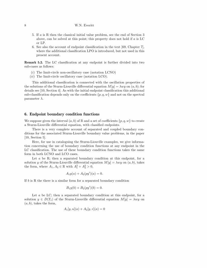
5. If a is R then the classical initial value problem, see the end of Section 3above, can be solved at this point; this property does not hold if a is LCor LP.
6. See also the account of endpoint classification in the text [69, Chapter 7],where the additional classification LPO is introduced, but not used in thispresent account.
Remark 5.2. The LC classification at any endpoint is further divided into twosub-cases as follows:
(i) The limit-circle non-oscillatory case (notation LCNO)(ii) The limit-circle oscillatory case (notation LCO).
This additional classification is connected with the oscillation properties ofthe solutions of the Sturm-Liouville differential equation M [y] = λwy on (a, b); fordetails see [10, Section 4]. As with the initial endpoint classification this additionalsub-classification depends only on the coefficients {p, q, w} and not on the spectralparameter λ.
6. Endpoint boundary condition functions
We suppose given the interval (a, b) of R and a set of coefficients {p, q, w} to createa Sturm-Liouville differential equation, with classified endpoints.
There is a very complete account of separated and coupled boundary con-ditions for the associated Sturm-Liouville boundary value problems, in the paper[10, Section 5].
Here, for use in cataloguing the Sturm-Liouville examples, we give informa-tion concerning the use of boundary condition functions at any endpoint in theLC classification. The use of these boundary condition functions takes the sameform in both LCNO and LCO cases.
Let a be R; then a separated boundary condition at this endpoint, for asolution y of the Sturm-Liouville differential equation M [y] = λwy on (a, b), takesthe form, where A1, A2 ∈ R with A2
1 +A22 > 0,
A1y(a) +A2(py′)(a) = 0.
If b is R the there is a similar form for a separated boundary condition
B1y(b) +B2(py′)(b) = 0.
Let a be LC; then a separated boundary condition at this endpoint, for asolution y ∈ D(T1) of the Sturm-Liouville differential equation M [y] = λwy on(a, b), takes the form,
A1[y, u](a) +A2[y, v](a) = 0

Sturm-Liouville differential equations 9
where(i) A1, A2 ∈ R with A2
1 +A22 > 0
(ii) u, v : (a, b)→ R
(iii) u, v ∈ D(T1)(iv) [u, v](a) 6= 0.
Such pairs {u, v} of elements from the maximal domain D(T1) always exist underthe LC classification on the endpoint a, see [10, Section 5].
If b is LC then there is a similar form for a separated boundary conditioninvolving a pair {u, v} of boundary condition functions, in general a different pairfrom the pair required for the endpoint a, to give
B1[y, u](b) +B2[y, v](b) = 0.
For any given particular Sturm-Liouville differential equation the search forpairs of such boundary condition functions may start with a study of the solutionsof the differential equation M [y] = λwy on (a, b), and also with a direct searchwithin the elements of the maximal domain D(T1).
For the examples given in the catalogue a suitable choice of these boundarycondition functions is given, for endpoints in the LC case.
Remark 6.1. In practice it is sufficient to determine the pair {u, v} in a neigh-bourhood (a, c] of a, or [c, b) of b, so that they are locally in the maximal domainD(T1); this practice is adopted in many of the examples given in this catalogue.
7. The Liouville transformation
The named Liouville transformation, see [30, Section 4.3] and [17, Chapter 10,Section 10] for details, of the general Sturm-Liouville differential equation
−(p(x)y′(x))′ + q(x)y(x) = λw(x)y(x) for all x ∈ (a, b)
provides a means, under additional conditions on the coefficients {p, q, w}, to yielda simpler Sturm-Liouville form of the differential equation
−Y ′′(X) +Q(X)Y (X) = λY (X) for all X ∈ (A,B).
The minimal additional conditions required, see [30, Section 4.3], are
(i) p and p′ ∈ ACloc(a, b), and p(x) > 0 for all x ∈ (a, b)(ii) w and w′ ∈ ACloc(a, b), and w(x) > 0 for all x ∈ (a, b).
The Liouville transformation changes the variables x and y to X and Y asfollows, see [30, Section 4.3]:

10 W.N. Everitt
(i) For k ∈ (a, b) and K ∈ R the mapping X(·) : (a, b) → (A,B) defines anew independent variable X(·) by
X(x) = l(x) := K +∫ x
k
{w(t)/p(t)}1/2 dt for all x ∈ (a, b)
A := K −∫ k
a
{w(t)/p(t)}1/2 dt and B := K +∫ b
k
{w(t)/p(t)}1/2 dt
where −∞ ≤ A < B ≤ +∞; there is then an inverse mapping L(·) :(A,B)→ (a, b).
(ii) Define the new dependent variable Y (·) by
Y (X) := {p(x)w(x)}1/4y(x) for all x ∈ (a, b)
:= {p(L(X))w(L(X))}1/4y(L(X)) for all X ∈ (A,B).
The new coefficient Q is given by
Q(X) = w(x)−1q(x)− {w(x)−3p(x)}1/4(p(x)({p(x)w(x)}−1/4)′)′ for all x ∈ (a, b).
An example of this Liouville transformation is worked in Section 11 for oneform of the Bessel equation.
8. Fourier equation
This is the classical Sturm-Liouville differential equation, see [78, Chapter I, andChapter IV, Section 4.1],
−y′′(x) = λy(x) for all x ∈ (−∞,+∞)
with solutionscos(x
√λ) and sin(x
√λ).
Endpoint classification in L2(−∞,+∞):
Endpoint Classification−∞ LP
0 R+∞ LP
This is a simple constant coefficient equation; for any self-adjoint bound-ary value problem on a compact interval the eigenvalues can be characterized interms of the solutions of a transcendental equation involving only trigonometricfunctions.
For a study of boundary value problems on the half-line [0,∞) or the wholeline (−∞,∞) see [78, Chapter IV, Section 4.1] and [2, Volume II, Appendix 2,Section 132, Part 2].

Sturm-Liouville differential equations 11
9. Hypergeometric equation
The standard form for this differential equation is, see [46, Chapter 4, Section3], [80, Chapter XIV, Section 14.2], [16, Chapter 9, Section 9.2], [27, Chapter II,Section 2.1.1], [1, Chapter 15, Section 15.5] and [78, Chapter IV, Sections 4.18 to4.20],
z(1− z)y′′(z) + [c− (a+ b+ 1)z]y′(z)− aby(z) = 0 for all z ∈ C
where, in general a, b, c ∈ C. In terms of the hypergeometric function 2F1, so-lutions of this equation are, with certain restrictions on the parameters and theindependent variable z,
2F1(a, b; c; z) and z1−c2F1(a+ 1− c, b+ 1− c; 2− c; z).
For consideration of this hypergeometric equation in Sturm-Liouville form wereplace the variable z by the real variable x ∈ (0, 1). Thereafter, on multiplying bythe factor xα(1−x)β and rearranging the terms gives the Sturm-Liouville equation,for all α, β ∈ R,
−(xα+1(1− x)β+1y′(x)
)′= λxα(1− x)βy(x) for all x ∈ (0, 1).
In this form the relationship between the parameters {a, b, c} and {α, β, λ} is
c = α+ 1 a+ b = α+ β + 1 ab = −λ;
these equations can be solved for {a, b, c} in terms of {α, β, λ} as in [78, ChapterIV, Section 4.18].
Given α, β ∈ R and λ ∈ C the solutions of this Sturm-Liouville equation canthen be represented in terms of the hypergeometric function 2F1, as above.
For the case when λ = 0 the general solution of this differential equationtakes the form, for c ∈ (0, 1),
y(x) = k
∫ x
c
1tα+1(1− t)β+1
dt+ l for all x ∈ (0, 1)
where the numbers k, l ∈ C. From this representation it may be shown that thefollowing classifications, in the space L2((0, 1);xα(1−x)β), of the endpoints 0 and1 hold:
Endpoint Parameters α, β Classification0 For α ∈ (−1, 0) and all β ∈ R R0 For α ∈ [0, 1) and all β ∈ R LCNO0 For α ∈ (−∞,−1] ∪ [1,∞) and all β ∈ R LP1 For β ∈ (−1, 0) and all α ∈ R R1 For β ∈ [0, 1) and all α ∈ R LCNO1 For β ∈ (−∞,−1] ∪ [1,∞) and all α ∈ R LP

12 W.N. Everitt
For the endpoint 0, for α ∈ [0, 1) and for all β ∈ R the LCNO boundarycondition functions u, v take the form, for all x ∈ (0, 1),
Parameter u vα = 0 1 ln(x)
α ∈ (0, 1) 1 x−α
For the endpoint 1, for β ∈ [0, 1) and for all α ∈ R the LCNO boundarycondition functions u, v take the form, for all x ∈ (0, 1),
Parameter u vβ = 0 1 ln(1− x)
β ∈ (0, 1) 1 (1− x)−β
Another form of the hypergeometric differential equation is obtained if in theoriginal equation above the independent variable z is replaced by −z to give
z(1 + z)y′′(z) + [c+ (a+ b+ 1)z]y′(z) + aby(z) = 0 for all z ∈ C
with general solutions
2F1(a, b; c;−z) and z1−c2F1(a+ 1− c, b+ 1− c; 2− c;−z);
see the account in [78, Chapter IV, Section 4.18].For consideration of this hypergeometric equation in Sturm-Liouville form we
replace the variable z by the real variable x ∈ (0,∞). Thereafter, on multiplyingby the factor xα(1 + x)β and re-arranging the terms gives the Sturm-Liouvilleequation, for all α, β ∈ R,
−(xα+1(1 + x)β+1y′(x)
)′= λxα(1 + x)βy(x) for all x ∈ (0,∞).
In this form the relationship between the parameters {a, b, c} and {α, β, λ} is
c = α+ 1 a+ b = α+ β + 1 ab = λ;
these equations can be solved for {a, b, c} in terms of {α, β, λ} as in [78, ChapterIV, Section 4.18].
Given α, β ∈ R and λ ∈ C the solutions of this Sturm-Liouville equation canthen be represented in terms of the hypergeometric function 2F1, as above.
For the case when λ = 0 the general solution of this differential equationtakes the form, for c ∈ (0,∞),
y(x) = k
∫ x
c
1tα+1(1 + t)β+1
dt+ l for all x ∈ (0,∞)
where the numbers k, l ∈ C. From this representation it may be shown that thefollowing classifications, in the space L2((0,∞);xα(1 + x)β), of the endpoints 0
Sturm-Liouville differential equations 13
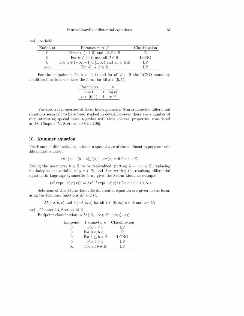
and +∞ hold:
Endpoint Parameters α, β Classification0 For α ∈ (−1, 0) and all β ∈ R R0 For α ∈ [0, 1) and all β ∈ R LCNO0 For α ∈ (−∞,−1] ∪ [1,∞) and all β ∈ R LP
+∞ For all α, β ∈ R LP
For the endpoint 0, for α ∈ [0, 1) and for all β ∈ R the LCNO boundarycondition functions u, v take the form, for all x ∈ (0, 1),
Parameter u vα = 0 1 ln(x)
α ∈ (0, 1) 1 x−α
The spectral properties of these hypergeometric Sturm-Liouville differentialequations seem not to have been studied in detail; however there are a number ofvery interesting special cases, together with their spectral properties, consideredin [78, Chapter IV, Sections 4.18 to 4.20].
10. Kummer equation
The Kummer differential equation is a special case of the confluent hypergeometricdifferential equation
zw′′(z) + (b− z)y′(z)− aw(z) = 0 for z ∈ C.
Taking the parameter b ∈ R to be real-valued, putting λ = −a ∈ C, replacingthe independent variable z by x ∈ R, and then writing the resulting differentialequation in Lagrange symmetric form, gives the Sturm-Liouville example
−(xb exp(−x)y′(x))′ = λxb−1 exp(−x)y(x) for all x ∈ (0,∞).
Solutions of this Sturm-Liouville differential equation are given in the form,using the Kummer functions M and U,
M(−λ, b, x) and U(−λ, b, x) for all x ∈ (0,∞), b ∈ R and λ ∈ C;
see[1, Chapter 13, Section 13.1].Endpoint classification in L2((0,+∞);xb−1 exp(−x)):
Endpoint Parameter b Classification0 For b ≤ 0 LP0 For 0 < b < 1 R0 For 1 ≤ b < 2 LCNO0 For b ≥ 2 LP∞ For all b ∈ R LP
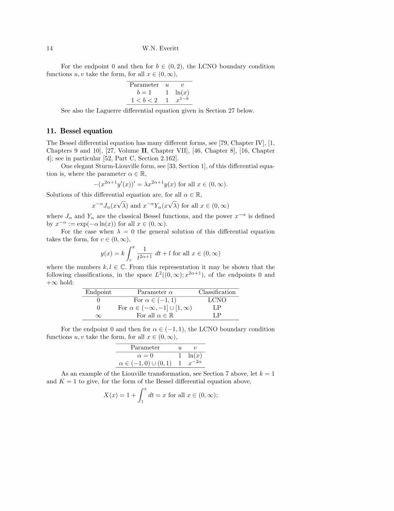
14 W.N. Everitt
For the endpoint 0 and then for b ∈ (0, 2), the LCNO boundary conditionfunctions u, v take the form, for all x ∈ (0,∞),
Parameter u vb = 1 1 ln(x)
1 < b < 2 1 x1−b
See also the Laguerre differential equation given in Section 27 below.
11. Bessel equation
The Bessel differential equation has many different forms, see [79, Chapter IV], [1,Chapters 9 and 10], [27, Volume II, Chapter VII], [46, Chapter 8], [16, Chapter4]; see in particular [52, Part C, Section 2.162].
One elegant Sturm-Liouville form, see [33, Section 1], of this differential equa-tion is, where the parameter α ∈ R,
−(x2α+1y′(x))′ = λx2α+1y(x) for all x ∈ (0,∞).
Solutions of this differential equation are, for all α ∈ R,x−αJα(x
√λ) and x−αYα(x
√λ) for all x ∈ (0,∞)
where Jα and Yα are the classical Bessel functions, and the power x−α is definedby x−α := exp(−α ln(x)) for all x ∈ (0,∞).
For the case when λ = 0 the general solution of this differential equationtakes the form, for c ∈ (0,∞),
y(x) = k
∫ x
c
1t2α+1
dt+ l for all x ∈ (0,∞)
where the numbers k, l ∈ C. From this representation it may be shown that thefollowing classifications, in the space L2((0,∞);x2α+1), of the endpoints 0 and+∞ hold:
Endpoint Parameter α Classification0 For α ∈ (−1, 1) LCNO0 For α ∈ (−∞,−1] ∪ [1,∞) LP∞ For all α ∈ R LP
For the endpoint 0 and then for α ∈ (−1, 1), the LCNO boundary conditionfunctions u, v take the form, for all x ∈ (0,∞),
Parameter u vα = 0 1 ln(x)
α ∈ (−1, 0) ∪ (0, 1) 1 x−2α
As an example of the Liouville transformation, see Section 7 above, let k = 1and K = 1 to give, for the form of the Bessel differential equation above,
X(x) = 1 +∫ x
1
dt = x for all x ∈ (0,∞);
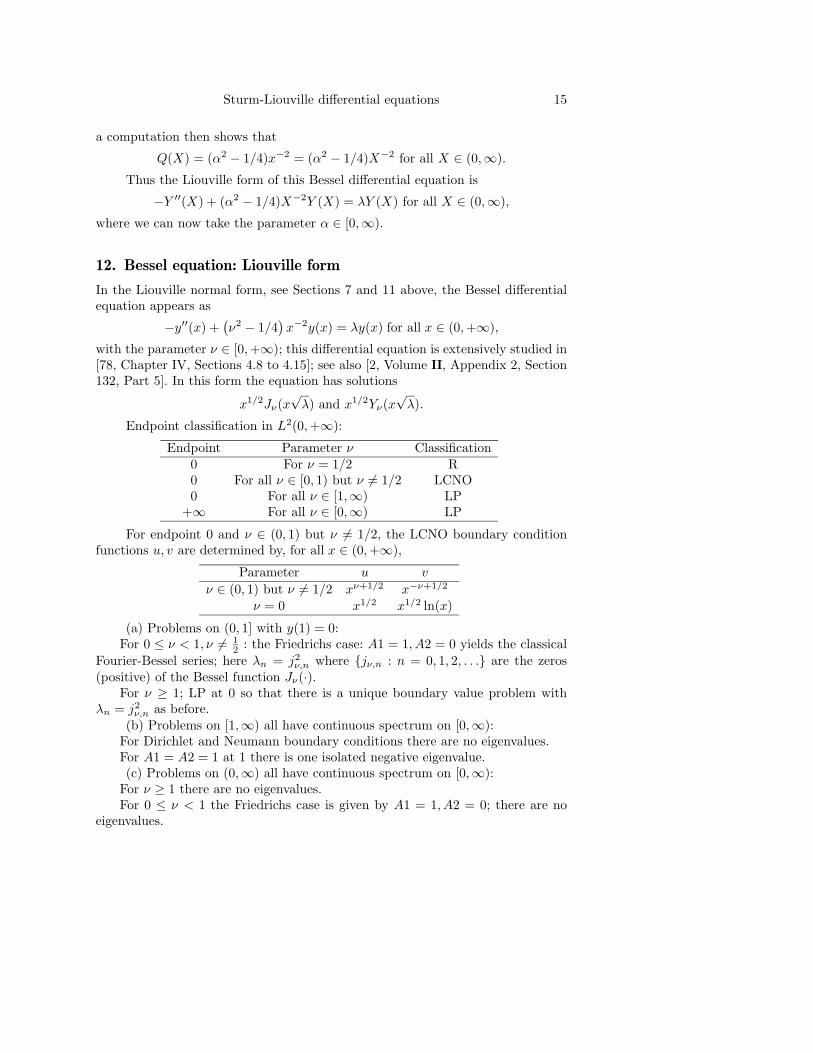
Sturm-Liouville differential equations 15
a computation then shows that
Q(X) = (α2 − 1/4)x−2 = (α2 − 1/4)X−2 for all X ∈ (0,∞).
Thus the Liouville form of this Bessel differential equation is
−Y ′′(X) + (α2 − 1/4)X−2Y (X) = λY (X) for all X ∈ (0,∞),
where we can now take the parameter α ∈ [0,∞).
12. Bessel equation: Liouville form
In the Liouville normal form, see Sections 7 and 11 above, the Bessel differentialequation appears as
−y′′(x) +(ν2 − 1/4
)x−2y(x) = λy(x) for all x ∈ (0,+∞),
with the parameter ν ∈ [0,+∞); this differential equation is extensively studied in[78, Chapter IV, Sections 4.8 to 4.15]; see also [2, Volume II, Appendix 2, Section132, Part 5]. In this form the equation has solutions
x1/2Jν(x√λ) and x1/2Yν(x
√λ).
Endpoint classification in L2(0,+∞):
Endpoint Parameter ν Classification0 For ν = 1/2 R0 For all ν ∈ [0, 1) but ν 6= 1/2 LCNO0 For all ν ∈ [1,∞) LP
+∞ For all ν ∈ [0,∞) LP
For endpoint 0 and ν ∈ (0, 1) but ν 6= 1/2, the LCNO boundary conditionfunctions u, v are determined by, for all x ∈ (0,+∞),
Parameter u v
ν ∈ (0, 1) but ν 6= 1/2 xν+1/2 x−ν+1/2
ν = 0 x1/2 x1/2 ln(x)
(a) Problems on (0, 1] with y(1) = 0:For 0 ≤ ν < 1, ν 6= 1
2 : the Friedrichs case: A1 = 1, A2 = 0 yields the classicalFourier-Bessel series; here λn = j2
ν,n where {jν,n : n = 0, 1, 2, . . .} are the zeros(positive) of the Bessel function Jν(·).
For ν ≥ 1; LP at 0 so that there is a unique boundary value problem withλn = j2
ν,n as before.(b) Problems on [1,∞) all have continuous spectrum on [0,∞):
For Dirichlet and Neumann boundary conditions there are no eigenvalues.For A1 = A2 = 1 at 1 there is one isolated negative eigenvalue.(c) Problems on (0,∞) all have continuous spectrum on [0,∞):
For ν ≥ 1 there are no eigenvalues.For 0 ≤ ν < 1 the Friedrichs case is given by A1 = 1, A2 = 0; there are no
eigenvalues.
16 W.N. Everitt
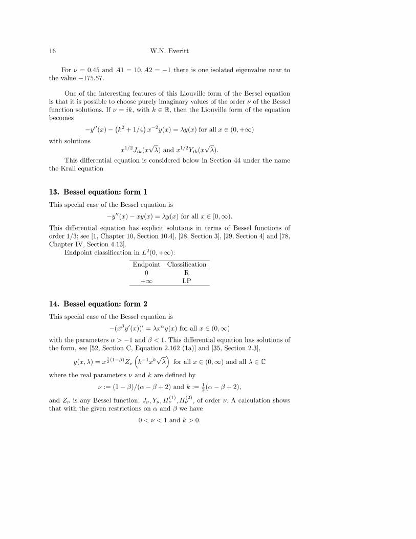
For ν = 0.45 and A1 = 10, A2 = −1 there is one isolated eigenvalue near tothe value −175.57.
One of the interesting features of this Liouville form of the Bessel equationis that it is possible to choose purely imaginary values of the order ν of the Besselfunction solutions. If ν = ik, with k ∈ R, then the Liouville form of the equationbecomes
−y′′(x)−(k2 + 1/4
)x−2y(x) = λy(x) for all x ∈ (0,+∞)
with solutionsx1/2Jik(x
√λ) and x1/2Yik(x
√λ).
This differential equation is considered below in Section 44 under the namethe Krall equation
13. Bessel equation: form 1
This special case of the Bessel equation is
−y′′(x)− xy(x) = λy(x) for all x ∈ [0,∞).
This differential equation has explicit solutions in terms of Bessel functions oforder 1/3; see [1, Chapter 10, Section 10.4], [28, Section 3], [29, Section 4] and [78,Chapter IV, Section 4.13].
Endpoint classification in L2(0,+∞):
Endpoint Classification0 R
+∞ LP
14. Bessel equation: form 2
This special case of the Bessel equation is
−(xβy′(x))′ = λxαy(x) for all x ∈ (0,∞)
with the parameters α > −1 and β < 1. This differential equation has solutions ofthe form, see [52, Section C, Equation 2.162 (1a)] and [35, Section 2.3],
y(x, λ) = x12 (1−β)Zν
(k−1xk
√λ)
for all x ∈ (0,∞) and all λ ∈ C
where the real parameters ν and k are defined by
ν := (1− β)/(α− β + 2) and k := 12 (α− β + 2),
and Zν is any Bessel function, Jν , Yν ,H(1)ν ,H
(2)ν , of order ν. A calculation shows
that with the given restrictions on α and β we have
0 < ν < 1 and k > 0.

Sturm-Liouville differential equations 17
Endpoint classification in L2(0,+∞;xα), for all α and β as above,
Endpoint Classification0 R
+∞ LP
15. Bessel equation: form 3
This special case of the Bessel equation is
−(xτy′(x))′ = λy(x) for all x ∈ [1,∞).
where the real parameter τ ∈ (−∞,∞). This differential equation has solutions ofthe form, see [52, Section C, Equation 2.162] and [32, Section 5],
y(x, λ) = x12 (1−τ)Zv
(2(2− τ)−1x
12 (2−τ)
√λ)
for all x ∈ [1,∞) and all λ ∈ C
where the real parameter ν is defined by
ν := (1− τ)/(2− τ) ,
and where Zν is any Bessel function, Jν , Yν ,H(1)ν ,H
(2)ν , of order ν.
Endpoint classification in L2(1,∞), for all τ ∈ (−∞,∞),
Endpoint Classification1 R
+∞ LP
16. Bessel equation: form 4
This special case of the Bessel equation is, with a > 0,
−y′′(x) + (ν2 − 1/4)x−2y(x) = λy(x) for all x ∈ [a,∞).
This equation is a special case of the Liouville form of the Bessel differentialequation, see Section 12 above, with the parameter ν ≥ 0 and considered on theinterval [a,∞) to avoid the singularity at the endpoint 0. The reason for thischoice of endpoint is to relate to the Weber integral transform as considered in[78, Chapter IV, Section 4.10]. As in Section 12 above this equation has solutions
x1/2Jν(x√λ) and x1/2Yν(x
√λ) for all x ∈ [a,∞)
but now the endpoint classification in L2[a,∞) is
Endpoint Classificationa R
+∞ LP

18 W.N. Everitt
17. Bessel equation: modified form
The modified Bessel functions, notation Iν and Kν , are best defined, on the realline R, in terms of the classical Bessel functions Jν and Yν by, see [16, Chapter 4,Section 4.7],
Iν(x) := i−νJν(ix) and Kν(x) :=π
2iν+1{Jν(ix) + iYν(ix)} for all x ∈ R.
The properties of these special functions are considered in [16, Chapter 4, Section4.7 to 4.9].
With careful attention to the branch definition of the powers of the factorsiν it may be shown that
Iν(·) : R→ R and Kν(·) : R→ R.
The functions Iν(x√λ) and Kν(x
√λ) form an independent basis of solutions
for the differential equation
(xy′(x))′ − ν2x−1y(x) = λxy(x) for all x ∈ (0,∞)
and have properties similar to the classical Bessel functions Jν(x√λ) and Yν(x
√λ),
respectively, when x ∈ R and λ ∈ C.If the Liouville transformation is applied to this last equation, or in the Bessel
Liouville differential equation, see Section 12 above, the formal transformationx 7−→ ix is applied, then the resulting differential equation has the form
y′′(x)−(ν2 − 1/4
)x−2y(x) = λy(x) for all x ∈ (0,+∞).
This gives one interesting property of the Liouville form of the differential equationfor the modified Bessel functions; in the standard Sturm-Liouville form given inSection 2 above the leading coefficient p has to be taken as negative valued on theinterval (0,∞), i.e.
p(x) = −1 q(x) = −(ν2 − 1/4
)x−2 w(x) = 1 for all x ∈ (0,∞).
The independent solutions of this Liouville form are
x1/2Iν(x√λ) and x1/2Kν(x
√λ) for all x ∈ (0,∞).
Endpoint classification in L2(0,+∞):
Endpoint Parameter ν Classification0 For ν = 1/2 R0 For all ν ∈ [0, 1) but ν 6= 1/2 LCNO0 For all ν ∈ [1,∞) LP
+∞ For all ν ∈ [0,∞) LP
For endpoint 0 and ν ∈ (0, 1) but ν 6= 1/2, the LCNO boundary conditionfunctions u, v are determined by, for all x ∈ (0,+∞),
Parameter u v
ν ∈ (0, 1) but ν 6= 1/2 xν+1/2 x−ν+1/2
ν = 0 x1/2 x1/2 ln(x)
Sturm-Liouville differential equations 19
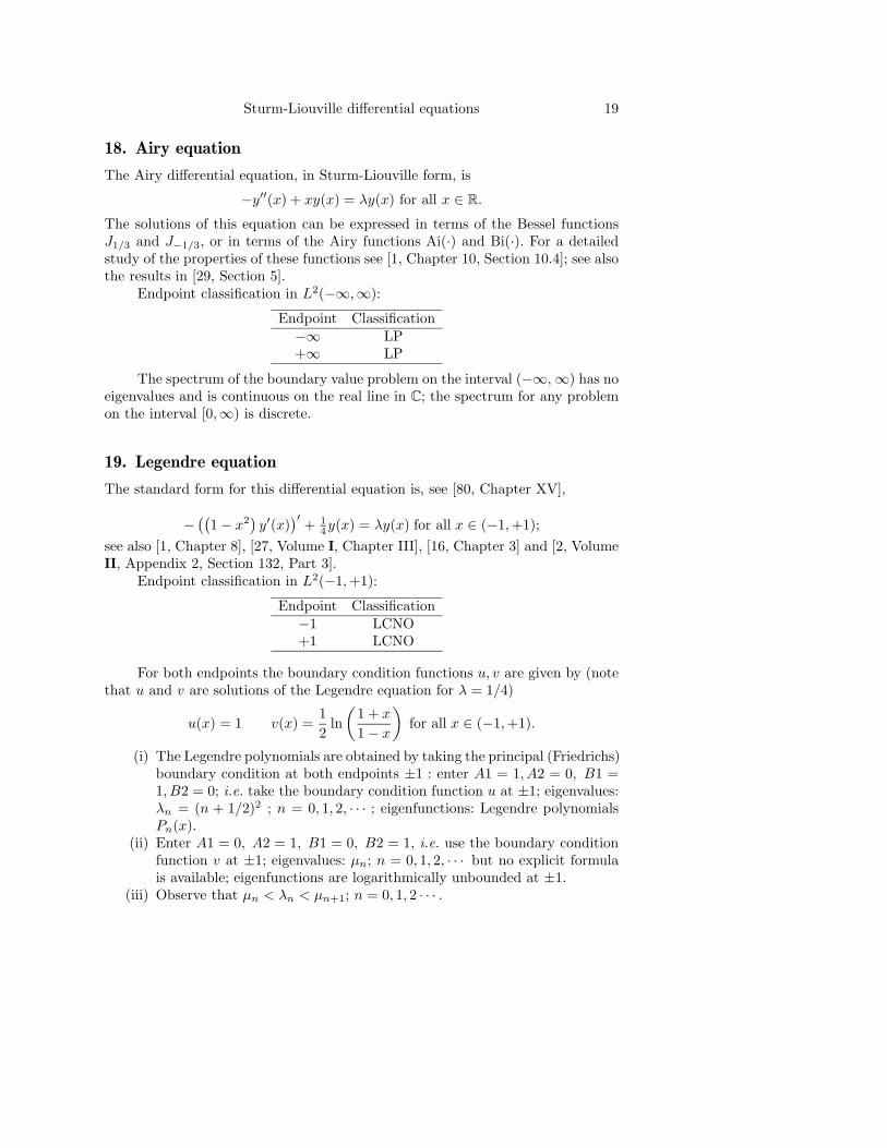
18. Airy equation
The Airy differential equation, in Sturm-Liouville form, is
−y′′(x) + xy(x) = λy(x) for all x ∈ R.The solutions of this equation can be expressed in terms of the Bessel functionsJ1/3 and J−1/3, or in terms of the Airy functions Ai(·) and Bi(·). For a detailedstudy of the properties of these functions see [1, Chapter 10, Section 10.4]; see alsothe results in [29, Section 5].
Endpoint classification in L2(−∞,∞):
Endpoint Classification−∞ LP+∞ LP
The spectrum of the boundary value problem on the interval (−∞,∞) has noeigenvalues and is continuous on the real line in C; the spectrum for any problemon the interval [0,∞) is discrete.
19. Legendre equation
The standard form for this differential equation is, see [80, Chapter XV],
−((
1− x2)y′(x)
)′+ 1
4y(x) = λy(x) for all x ∈ (−1,+1);see also [1, Chapter 8], [27, Volume I, Chapter III], [16, Chapter 3] and [2, VolumeII, Appendix 2, Section 132, Part 3].
Endpoint classification in L2(−1,+1):
Endpoint Classification−1 LCNO+1 LCNO
For both endpoints the boundary condition functions u, v are given by (notethat u and v are solutions of the Legendre equation for λ = 1/4)
u(x) = 1 v(x) =12
ln(
1 + x
1− x
)for all x ∈ (−1,+1).
(i) The Legendre polynomials are obtained by taking the principal (Friedrichs)boundary condition at both endpoints ±1 : enter A1 = 1, A2 = 0, B1 =1, B2 = 0; i.e. take the boundary condition function u at ±1; eigenvalues:λn = (n + 1/2)2 ; n = 0, 1, 2, · · · ; eigenfunctions: Legendre polynomialsPn(x).
(ii) Enter A1 = 0, A2 = 1, B1 = 0, B2 = 1, i.e. use the boundary conditionfunction v at ±1; eigenvalues: µn; n = 0, 1, 2, · · · but no explicit formulais available; eigenfunctions are logarithmically unbounded at ±1.
(iii) Observe that µn < λn < µn+1; n = 0, 1, 2 · · · .
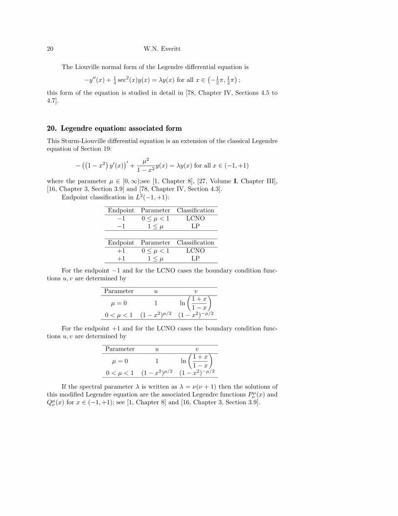
20 W.N. Everitt
The Liouville normal form of the Legendre differential equation is
−y′′(x) + 14 sec2(x)y(x) = λy(x) for all x ∈
(− 1
2π,12π)
;
this form of the equation is studied in detail in [78, Chapter IV, Sections 4.5 to4.7].
20. Legendre equation: associated form
This Sturm-Liouville differential equation is an extension of the classical Legendreequation of Section 19:
−((
1− x2)y′(x)
)′+
µ2
1− x2y(x) = λy(x) for all x ∈ (−1,+1)
where the parameter µ ∈ [0,∞);see [1, Chapter 8], [27, Volume I, Chapter III],[16, Chapter 3, Section 3.9] and [78, Chapter IV, Section 4.3].
Endpoint classification in L2(−1,+1):
Endpoint Parameter Classification−1 0 ≤ µ < 1 LCNO−1 1 ≤ µ LP
Endpoint Parameter Classification+1 0 ≤ µ < 1 LCNO+1 1 ≤ µ LP
For the endpoint −1 and for the LCNO cases the boundary condition func-tions u, v are determined by
Parameter u v
µ = 0 1 ln(
1 + x
1− x
)0 < µ < 1 (1− x2)µ/2 (1− x2)−µ/2
For the endpoint +1 and for the LCNO cases the boundary condition func-tions u, v are determined by
Parameter u v
µ = 0 1 ln(
1 + x
1− x
)0 < µ < 1 (1− x2)µ/2 (1− x2)−µ/2
If the spectral parameter λ is written as λ = ν(ν + 1) then the solutions ofthis modified Legendre equation are the associated Legendre functions Pµν (x) andQµν (x) for x ∈ (−1,+1); see [1, Chapter 8] and [16, Chapter 3, Section 3.9].
Sturm-Liouville differential equations 21
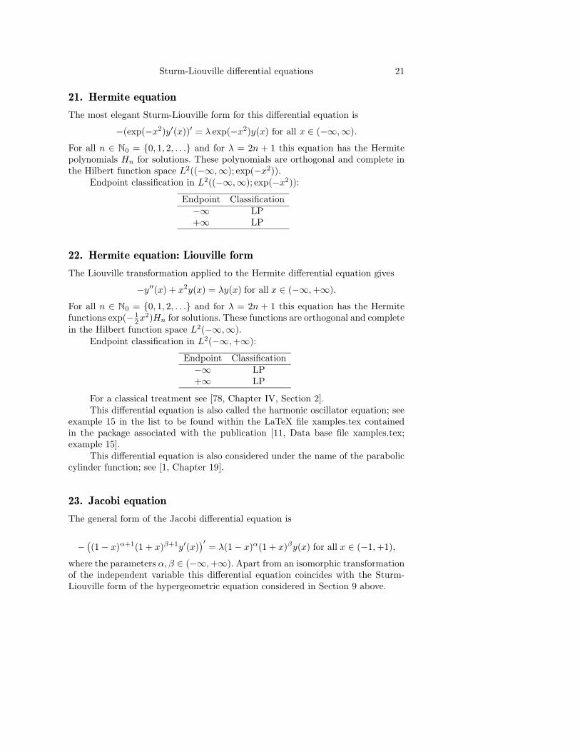
21. Hermite equation
The most elegant Sturm-Liouville form for this differential equation is
−(exp(−x2)y′(x))′ = λ exp(−x2)y(x) for all x ∈ (−∞,∞).
For all n ∈ N0 = {0, 1, 2, . . .} and for λ = 2n + 1 this equation has the Hermitepolynomials Hn for solutions. These polynomials are orthogonal and complete inthe Hilbert function space L2((−∞,∞); exp(−x2)).
Endpoint classification in L2((−∞,∞); exp(−x2)):
Endpoint Classification−∞ LP+∞ LP
22. Hermite equation: Liouville form
The Liouville transformation applied to the Hermite differential equation gives
−y′′(x) + x2y(x) = λy(x) for all x ∈ (−∞,+∞).
For all n ∈ N0 = {0, 1, 2, . . .} and for λ = 2n + 1 this equation has the Hermitefunctions exp(− 1
2x2)Hn for solutions. These functions are orthogonal and complete
in the Hilbert function space L2(−∞,∞).Endpoint classification in L2(−∞,+∞):
Endpoint Classification−∞ LP+∞ LP
For a classical treatment see [78, Chapter IV, Section 2].This differential equation is also called the harmonic oscillator equation; see
example 15 in the list to be found within the LaTeX file xamples.tex containedin the package associated with the publication [11, Data base file xamples.tex;example 15].
This differential equation is also considered under the name of the paraboliccylinder function; see [1, Chapter 19].
23. Jacobi equation
The general form of the Jacobi differential equation is
−((1− x)α+1(1 + x)β+1y′(x)
)′= λ(1− x)α(1 + x)βy(x) for all x ∈ (−1,+1),
where the parameters α, β ∈ (−∞,+∞). Apart from an isomorphic transformationof the independent variable this differential equation coincides with the Sturm-Liouville form of the hypergeometric equation considered in Section 9 above.

22 W.N. Everitt
Endpoint classification in the weighted space L2((−1,+1); (1−x)α(1+x)β)):
Endpoint Parameter Classification−1 β ≤ −1 LP−1 −1 < β < 0 R−1 0 ≤ β < 1 LCNO−1 1 ≤ β LP
Endpoint Parameter Classification+1 α ≤ −1 LP+1 −1 < α < 0 R+1 0 ≤ α < 1 LCNO+1 1 ≤ α LP
For the endpoint −1 and for the LCNO cases the boundary condition func-tions u, v are determined by
Parameter u v
β = 0 1 ln(
1 + x
1− x
)0 < β < 1 1 (1 + x)−β
For the endpoint +1 and for the LCNO cases the boundary condition func-tions u, v are determined by
Parameter u v
α = 0 1 ln(
1 + x
1− x
)0 < α < 1 1 (1− x)−α
To obtain the classical Jacobi orthogonal polynomials it is necessary to take−1 < α, β; then note the required boundary conditions:
Endpoint −1:
Parameter Boundary condition−1 < β < 0 (py′)(−1) = 0 or [y, v](−1) = 00 ≤ β < 1 [y, u](−1) = 0
Endpoint +1:
Parameter Boundary condition−1 < α < 0 (py′)(+1) = 0 or [y, v](+1) = 00 ≤ α < 1 [y, u](+1) = 0
For the classical Jacobi orthogonal polynomials the eigenvalues are given by:
λn = n(n+ α+ β + 1) for n = 0, 1, 2, . . .
and this explicit formula can be used to give an independent check on the accuracyof the results from the SLEIGN2 code.
Sturm-Liouville differential equations 23
It is interesting to note that the required boundary condition for these Jacobipolynomials is the Friedrichs condition in the LCNO cases.
In addition to the cases of the Jacobi equation mentioned in this section,there are other values of the parameters α and β which lead to important Sturm-Liouville differential equations; see the paper [53] and the book [3].
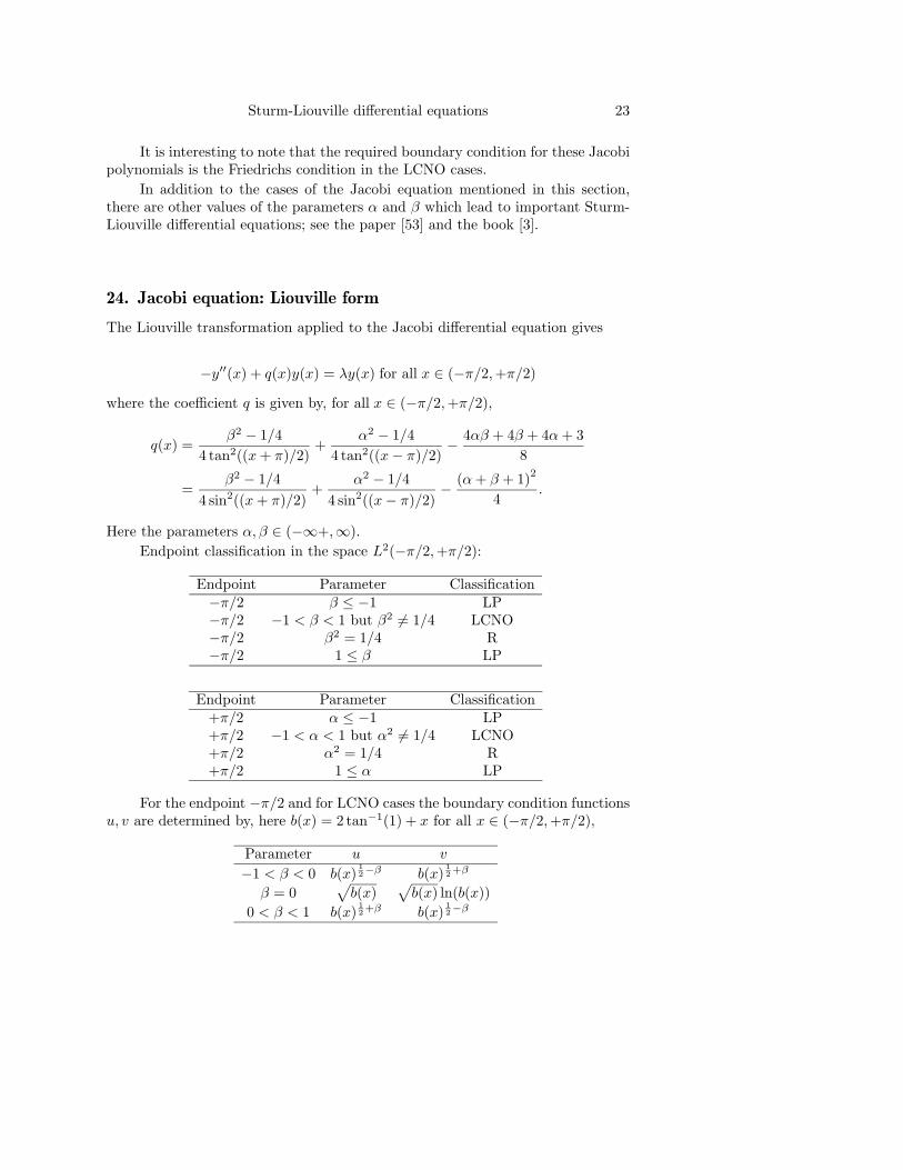
24. Jacobi equation: Liouville form
The Liouville transformation applied to the Jacobi differential equation gives
−y′′(x) + q(x)y(x) = λy(x) for all x ∈ (−π/2,+π/2)
where the coefficient q is given by, for all x ∈ (−π/2,+π/2),
q(x) =β2 − 1/4
4 tan2((x+ π)/2)+
α2 − 1/44 tan2((x− π)/2)
− 4αβ + 4β + 4α+ 38
=β2 − 1/4
4 sin2((x+ π)/2)+
α2 − 1/44 sin2((x− π)/2)
− (α+ β + 1)2
4.
Here the parameters α, β ∈ (−∞+,∞).Endpoint classification in the space L2(−π/2,+π/2):
Endpoint Parameter Classification−π/2 β ≤ −1 LP−π/2 −1 < β < 1 but β2 6= 1/4 LCNO−π/2 β2 = 1/4 R−π/2 1 ≤ β LP
Endpoint Parameter Classification+π/2 α ≤ −1 LP+π/2 −1 < α < 1 but α2 6= 1/4 LCNO+π/2 α2 = 1/4 R+π/2 1 ≤ α LP
For the endpoint −π/2 and for LCNO cases the boundary condition functionsu, v are determined by, here b(x) = 2 tan−1(1) + x for all x ∈ (−π/2,+π/2),
Parameter u v
−1 < β < 0 b(x)12−β b(x)
12 +β
β = 0√b(x)
√b(x) ln(b(x))
0 < β < 1 b(x)12 +β b(x)
12−β

24 W.N. Everitt
For the endpoint +π/2 and for LCNO cases the boundary condition functionsu, v are determined by, here a(x) = 2 tan−1(1)− x for all x ∈ (−π/2,+π/2),
Parameter u v
−1 < α < 0 a(x)12−α a(x)
12 +α
α = 0√a(x)
√a(x) ln(a(x))
0 < α < 1 a(x)12 +α a(x)
12−α
The classical Jacobi orthogonal polynomials are produced only when bothα, β > −1. For α, β > +1 the LP condition holds and no boundary condition isrequired to give the polynomials. If −1 < α, β < 1 then the LCNO condition holdsand boundary conditions are required to produce the Jacobi polynomials; theseconditions are as follows:
Endpoint −π/2
Parameter Boundary condition−1 < β < 0 [y, v](−π/2) = 00 ≤ β < 1 [y, u](−π/2) = 0
Endpoint +π/2
Parameter Boundary condition−1 < α < 0 [y, v](+π/2) = 00 ≤ α < 1 [y, u](+π/2) = 0
Recall from Section 23 for the classical orthogonal Jacobi polynomials theeigenvalues are given explicitly by:
λn = n(n+ α+ β + 1) for n = 0, 1, 2, . . .
25. Jacobi function equation
This is another Jacobi differential equation which corresponds to the hypergeo-metric differential equation considered over the half-line [0,∞), see the secondequation in Section 9 above, and the paper [37].
This equation is written in the form
−(ω(x)y′(x))′ − ρ2ω(x)y(x) = λω(x)y(x) for all x ∈ (0,∞)
where
(i) α ≥ β ≥ −1/2(ii) ρ = α+ β + 1
(iii) ω(x) ≡ ω(x)α,β = 22ρ(sinh(x))2α+1(cosh(x))2β+1 for all x ∈ (0,∞).

Sturm-Liouville differential equations 25
Endpoint classification, for all β ∈ [−1/2,∞), in L2((0,∞);ω):
Endpoint Parameter α Classification0 For α ∈ [−1/2, 0) R0 For α ∈ [0, 1) LCNO0 For α ∈ [1,∞) LP
+∞ For all α ∈ [−1/2,∞) LP
For the endpoint 0, for α ∈ [0, 1) and for all β ∈ [1/2,∞) the LCNO boundarycondition functions u, v take the form, for all x ∈ (0, 1),
Parameter u vα = 0 1 ln(x)
α ∈ (0, 1) 1 x−2α
26. Jacobi function equation: Liouville form
In the Liouville normal form, see Sections 7 and 11 above, the Jacobi functiondifferential equation of Section 25 above appears as
−y′′(x) + q(x)y(x) = λy(x) for all x ∈ (0,∞),
where the coefficient q is determined by, again with α ≥ β ≥ −1/2,
q(x) =α2 − 1/4(sinh(x))2
− β2 − 1/4(cosh(x))2
for all x ∈ (0,∞).
Endpoint classification, for all β ∈ [−1/2,∞), in L2(0,∞):
Endpoint Parameter α Classification0 For α = −1/2 R0 For α ∈ (−1/2, 1/2) LCNO0 For α = 1/2 R0 For α ∈ (1/2, 1) LCNO0 For α ∈ [1,∞) LP
+∞ For all α ∈ [−1/2,∞) LP
For the endpoint 0, for α ∈ [−1/2, 1) but |α| 6= 1/2 and for all β ∈ [−1/2,∞)the LCNO boundary condition functions u, v take the form, for all x ∈ (0, 1),
Parameter u v
α = 0 x1/2 x1/2 ln(x)α ∈ [−1/2, 1) but |α| 6= 1/2 x|α|+1/2 x−|α|+1/2
26 W.N. Everitt
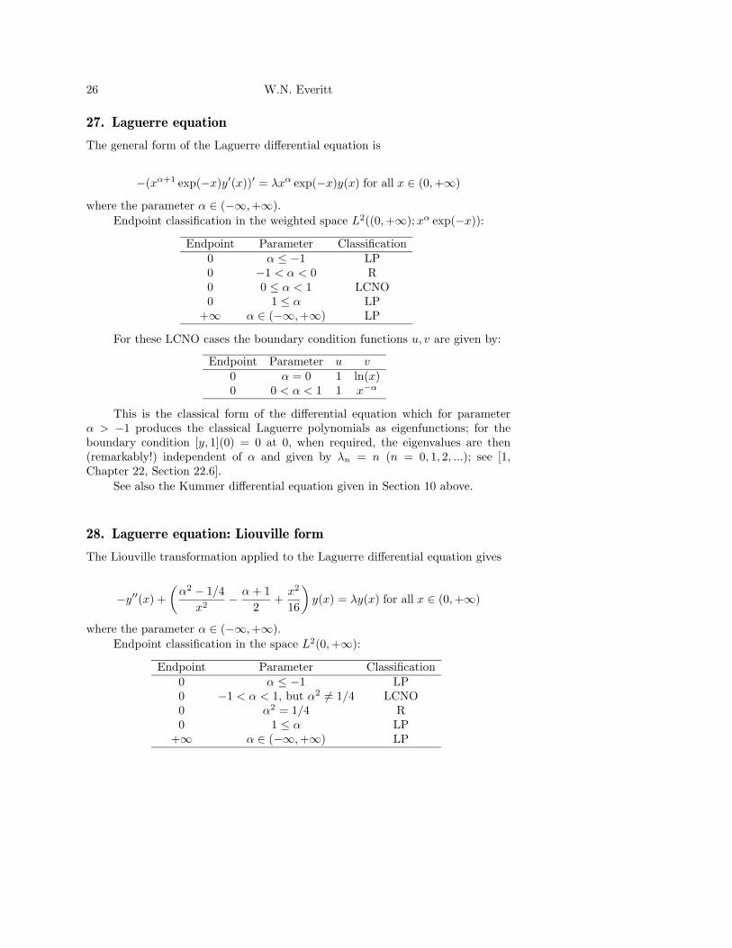
27. Laguerre equation
The general form of the Laguerre differential equation is
−(xα+1 exp(−x)y′(x))′ = λxα exp(−x)y(x) for all x ∈ (0,+∞)
where the parameter α ∈ (−∞,+∞).Endpoint classification in the weighted space L2((0,+∞);xα exp(−x)):
Endpoint Parameter Classification0 α ≤ −1 LP0 −1 < α < 0 R0 0 ≤ α < 1 LCNO0 1 ≤ α LP
+∞ α ∈ (−∞,+∞) LP
For these LCNO cases the boundary condition functions u, v are given by:
Endpoint Parameter u v0 α = 0 1 ln(x)0 0 < α < 1 1 x−α
This is the classical form of the differential equation which for parameterα > −1 produces the classical Laguerre polynomials as eigenfunctions; for theboundary condition [y, 1](0) = 0 at 0, when required, the eigenvalues are then(remarkably!) independent of α and given by λn = n (n = 0, 1, 2, ...); see [1,Chapter 22, Section 22.6].
See also the Kummer differential equation given in Section 10 above.
28. Laguerre equation: Liouville form
The Liouville transformation applied to the Laguerre differential equation gives
−y′′(x) +(α2 − 1/4
x2− α+ 1
2+x2
16
)y(x) = λy(x) for all x ∈ (0,+∞)
where the parameter α ∈ (−∞,+∞).Endpoint classification in the space L2(0,+∞):
Endpoint Parameter Classification0 α ≤ −1 LP0 −1 < α < 1, but α2 6= 1/4 LCNO0 α2 = 1/4 R0 1 ≤ α LP
+∞ α ∈ (−∞,+∞) LP
Sturm-Liouville differential equations 27
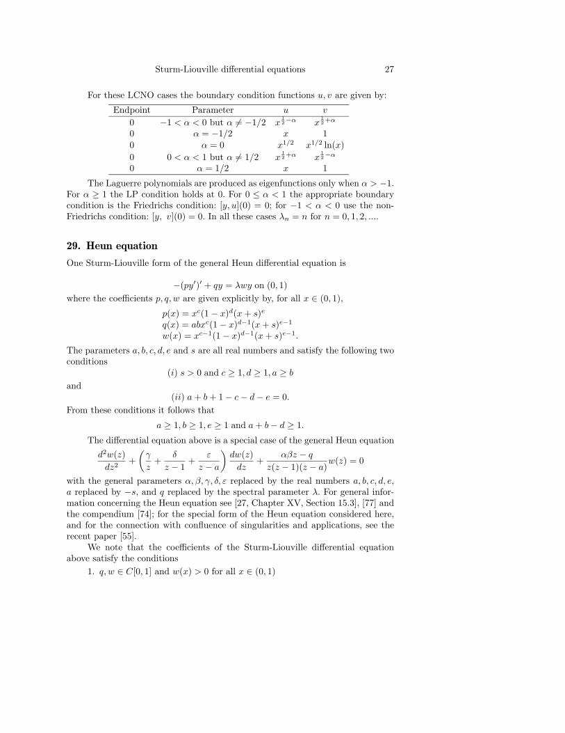
For these LCNO cases the boundary condition functions u, v are given by:
Endpoint Parameter u v
0 −1 < α < 0 but α 6= −1/2 x12−α x
12 +α
0 α = −1/2 x 10 α = 0 x1/2 x1/2 ln(x)0 0 < α < 1 but α 6= 1/2 x
12 +α x
12−α
0 α = 1/2 x 1
The Laguerre polynomials are produced as eigenfunctions only when α > −1.For α ≥ 1 the LP condition holds at 0. For 0 ≤ α < 1 the appropriate boundarycondition is the Friedrichs condition: [y, u](0) = 0; for −1 < α < 0 use the non-Friedrichs condition: [y, v](0) = 0. In all these cases λn = n for n = 0, 1, 2, ....
29. Heun equation
One Sturm-Liouville form of the general Heun differential equation is
−(py′)′ + qy = λwy on (0, 1)where the coefficients p, q, w are given explicitly by, for all x ∈ (0, 1),
p(x) = xc(1− x)d(x+ s)e
q(x) = abxc(1− x)d−1(x+ s)e−1
w(x) = xc−1(1− x)d−1(x+ s)e−1.
The parameters a, b, c, d, e and s are all real numbers and satisfy the following twoconditions
(i) s > 0 and c ≥ 1, d ≥ 1, a ≥ band
(ii) a+ b+ 1− c− d− e = 0.From these conditions it follows that
a ≥ 1, b ≥ 1, e ≥ 1 and a+ b− d ≥ 1.
The differential equation above is a special case of the general Heun equation
d2w(z)dz2
+(γ
z+
δ
z − 1+
ε
z − a
)dw(z)dz
+αβz − q
z(z − 1)(z − a)w(z) = 0
with the general parameters α, β, γ, δ, ε replaced by the real numbers a, b, c, d, e,a replaced by −s, and q replaced by the spectral parameter λ. For general infor-mation concerning the Heun equation see [27, Chapter XV, Section 15.3], [77] andthe compendium [74]; for the special form of the Heun equation considered here,and for the connection with confluence of singularities and applications, see therecent paper [55].
We note that the coefficients of the Sturm-Liouville differential equationabove satisfy the conditions
1. q, w ∈ C[0, 1] and w(x) > 0 for all x ∈ (0, 1)

28 W.N. Everitt
2. p−1 ∈ L1loc(0, 1), p(x) > 0 for all x ∈ (0, 1)
3. p−1 /∈ L1(0, 1/2] and p−1 /∈ L1[1/2, 1).
Thus both endpoints 0 and 1 are singular for the differential equation. Anal-ysis shows that the endpoint classification for this equation is
Endpoint Parameter Classification0 c ∈ [1, 2) LCNO0 c ∈ [2,+∞) LP1 d ∈ [1, 2) LCNO1 d ∈ [2,+∞) LP
For the endpoint 0 and for LCNO cases the boundary condition functionsu, v are determined by:
Parameter u vc = 1 1 ln(x)
1 < c < 2 1 x1−c
For the endpoint 1 and for LCNO cases the boundary condition functionsu, v are determined by:
Parameter u vd = 1 1 ln(1− x)
1 < d < 2 1 (1− x)1−d
Further it may be shown that the spectrum of any self-adjoint problem on(0, 1), with the parameters a, b, c, d, e and s satisfying the above conditions, andconsidered in the space L2((0, 1);w) with either separated or coupled boundaryconditions, is bounded below and discrete. For the analytic properties, and proofsof the spectral properties of this Heun differential equation, see the paper [7].
30. Whittaker equation
The general form of the Whittaker differential equation is
−y′′(x) +(
14
+k2 − 1x2
)y(x) = λ
1xy(x) for all x ∈ (0,+∞)
where the parameter k ∈ [1,+∞).Endpoint classification in the space L2(0,+∞;x−1), for all k ∈ [1,+∞):
Endpoint Classification0 LP
+∞ LP
This equation is studied in [49, Part II, Section 10], where there it is shownthat the LP case holds at +∞ and also at 0 for k ≥ 1; the general properties of

Sturm-Liouville differential equations 29
Whittaker functions are given in [1, Chapter 13, Section 13.1.31]. The spectrumof the boundary value problem on (0,∞) is discrete and is given explicitly by:
λn = n+ (k + 1)/2, n = 0, 1, 2, 3, . . . .
31. Lame equation
This differential equation has many forms; there is an extensive literature devotedto the definition, theory and properties of this equation and the associated Lamefunctions; see [80, Chapter XXIII, Section 23.4] and [27, Chapter XV, Section15.2]. The Lame equation is a special case of the Heun equation; see [27, ChapterXV, Section 15.3] and Section 29 above.
Here we consider two cases of the Lame equation involving the Weierstrassdouble periodic elliptic function ℘, considered for the special case when the fun-damental periods 2ω1 and 2ω2 of ℘ satisfy
ω1 ∈ (0,∞) and ω2 = iχ where χ ∈ (0,∞).
We note that the lattice of double poles for ℘ is rectangular with points [2mω1 +2nω2 : m,n ∈ Z} of C.
For the general theory of the Weierstrass elliptic function ℘ see [22, ChapterXIII] and [80, Chapter XX].
1. Consider the Sturm-Liouville differential equation
−y′′(x) + k℘(x)y(x) = λy(x) for all x ∈ (0, 2ω1)
where k is a real parameter, k ∈ R. We note that ℘(·) : (0, 2ω1) → R
and that ℘(·) ∈ L1loc(0, 2ω1); from [80, Chapter XX, Section 20.2] and [22,
Chapter XIII, Section 13.4] it follows that
℘(x) = x−2 +O(x2) as x→ 0+ and
℘(x) = (2ω1 − x)−2 +O((2ω1 − x)2) as x→ 2ω−1 .
These order results for the coefficient ℘, at the endpoints of the inter-val (0, 2ω1), taken together with the parameter k, allow of a comparisonbetween this form of the Lame equation and (a) the Liouville Bessel equa-tion of Section 12 when k ∈ [−1/4,+∞), and (b) the Krall equation ofSection 44 when k ∈ (−∞,−1/4). This comparison leads to the followingendpoint classification for this Lame equation in the space L2(0, 2ω1) :
Endpoint Parameter k Classification0 For k ∈ (−∞,−1/4) LCO0 For k ∈ [−1/4, 0) LCNO0 k = 0 R0 For k ∈ (0, 3/4) LCNO0 For k ∈ [3/4,∞) LP
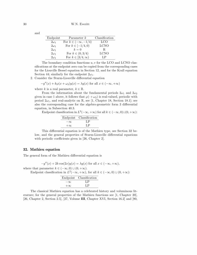
30 W.N. Everitt
andEndpoint Parameter k Classification
2ω1 For k ∈ (−∞,−1/4) LCO2ω1 For k ∈ [−1/4, 0) LCNO2ω1 k = 0 R2ω1 For k ∈ (0, 3/4) LCNO2ω1 For k ∈ [3/4,∞) LP
The boundary condition functions u, v for the LCO and LCNO clas-sifications at the endpoint zero can be copied from the corresponding casesfor the Liouville Bessel equation in Section 12, and for the Krall equationSection 44; similarly for the endpoint 2ω1.
2. Consider the Sturm-Liouville differential equation
−y′′(x) + k℘(x+ ω2)y(x) = λy(x) for all x ∈ (−∞,+∞)
where k is a real parameter, k ∈ R.From the information about the fundamental periods 2ω1 and 2ω2
given in case 1 above, it follows that ℘(·+ω2) is real-valued, periodic withperiod 2ω1, and real-analytic on R, see [1, Chapter 18, Section 18.1]; seealso the corresponding case for the algebro-geometric form 3 differentialequation, in Subsection 40.3.
Endpoint classification in L2(−∞,+∞) for all k ∈ (−∞, 0)∪(0,+∞):
Endpoint Classification−∞ LP+∞ LP
This differential equation is of the Mathieu type, see Section 32 be-low, and the general properties of Sturm-Liouville differential equationswith periodic coefficients given in [26, Chapter 2].
32. Mathieu equation
The general form of the Mathieu differential equation is
−y′′(x) + 2k cos(2x)y(x) = λy(x) for all x ∈ (−∞,+∞),where that parameter k ∈ (−∞, 0) ∪ (0,+∞).
Endpoint classification in L2(−∞,+∞), for all k ∈ (−∞, 0) ∪ (0,+∞):
Endpoint Classification−∞ LP+∞ LP
The classical Mathieu equation has a celebrated history and voluminous lit-erature; for the general properties of the Mathieu functions see [1, Chapter 20],[26, Chapter 2, Section 2.5], [27, Volume III, Chapter XVI, Section 16.2] and [80,

Sturm-Liouville differential equations 31
Chapter XIX, Sections 19.1 and 19.2]. For the general properties of Sturm-Liouvilledifferential equations with periodic coefficients see the text [26].
There are no eigenvalues for this problem on (−∞,+∞). There may be onenegative eigenvalue of the problem on [0,∞) depending on the boundary conditionat the endpoint 0. The continuous (essential) spectrum is the same for the wholeline or half-line problems and consists of an infinite number of disjoint closedintervals. The endpoints of these - and thus the spectrum of the problem - can becharacterized in terms of periodic and semi-periodic eigenvalues of Sturm-Liouvilleproblems on the compact interval [0, 2π]; these can be computed with SLEIGN2.
The above remarks also apply to the general Sturm-Liouville equation withperiodic coefficients of the same period; the so-called Hill’s equation.
Of special interest is the starting point of the continuous spectrum - this isalso the oscillation number of the equation. For the Mathieu equation (p = 1, q =cos(x), w = 1) on both the whole line and the half line it is approximately -0.378;this result may be obtained by computing the first eigenvalue λ0 of the periodicproblem on the interval [0, 2π].
For extensions of this theory to Sturm-Liouville differential equations withalmost periodic coefficients see the paper [60].
33. Bailey equation
The general form of the Bailey differential equation, see [11, Data base file xam-ples.tex; example 7], is
−(xy′(x))′ − x−1y(x) = λy(x) for all x ∈ (−∞, 0) ∪ (0,+∞).Endpoint classification in L2(−∞, 0)∪ L2(0,+∞):
Endpoint Classification−∞ LP0− LCO0+ LCO+∞ LP
For both endpoints 0− and 0+:
u(x) = cos (ln(|x|)) v(x) = sin (ln(|x|)) for all x ∈ (−∞, 0) ∪ (0,+∞).
This example is based on the earlier studied Sears-Titchmarsh equation; seeSection 58 below.
For numerical results see [11, Data base file xamples.tex; example 7].
34. Behnke-Goerisch equation
The general form of the Behnke-Goerisch differential equation, see [11, Data basefile xamples.tex; example 28], is

32 W.N. Everitt
−y′′(x) + k cos2(x)y(x) = λy(x) for all x ∈ (−∞,+∞)where the parameter k ∈ (−∞,+∞),
Endpoint classification in the space L2(−∞,+∞), for all k ∈ (−∞,+∞):
Endpoint Classification−∞ LP+∞ LP
This is a form of the Mathieu equation. In [15] these authors computed anumber of Neumann eigenvalues of this problem using interval arithmetic withrigorous bounds.
35. Boyd equation
The general form of the Boyd equation is, see [11, Data base file xamples.tex;example 4],
−y′′(x)− x−1y(x) = λy(x) for all x ∈ (−∞, 0) ∪ (0,+∞).Endpoint classification in L2(−∞, 0) ∪ L2(0,+∞):
Endpoint Classification−∞ LP0− LCNO0+ LCNO+∞ LP
For both endpoints 0− and 0+
u(x) = x v(x) = x ln(|x|) for all x ∈ (−∞, 0) ∪ (0,+∞).
This equation arises in a model studying eddies in the atmosphere; see [18].There is no explicit formula for the eigenvalues of any particular boundary condi-tion; eigenfunctions can be given in terms of Whittaker functions; see [8, Example3].
36. Boyd equation: regularized
The form of this regularized Boyd equation is
−(p(x)y′(x))′ + q(x)y(x) = λw(x)y(x) for all x ∈ (−∞, 0) ∪ (0,+∞)
wherep(x) = r(x)2 q(x) = −r(x)2 (ln(|x|)2
w(x) = r(x)2
withr(x) = exp (−(x ln(|x|)− x)) for all x ∈ (−∞, 0) ∪ (0,+∞).

Sturm-Liouville differential equations 33
Endpoint classification in L2(−∞, 0)∪ L2(0,+∞):
Endpoint Classification−∞ LP0− R0+ R+∞ LP
This is a regularized R form of the Boyd equation in Section 35; the LCNOsingularity at zero has been made R but requiring the introduction of quasi-derivatives. There is a close relationship between the examples these two formsof the Boyd equation; in particular they have the same eigenvalues - see [4]. Fora general discussion of regularization using non-principal solutions see [66]. Fornumerical results see [8, Example 3].
37. Dunford-Schwartz equation
This differential equation is considered in detail in [25, Chapter VIII, Pages 1515-20];
−((1− x2)y′(x)
)′+(
2α2
(1 + x)+
2β2
(1− x)
)y(x) = λy(x) for all x ∈ (−1,+1)
where the independent parameters α, β ∈ [0,+∞).Boundary value problems for this differential equation are discussed in [25,
Chapter XIII, Section 8].Endpoint classification in the space L2(−1,+1) for −1:
Parameter Classification0 ≤ α < 1/2 LCNO
1/2 ≤ α LP
Endpoint classification in the space L2(−1,+1) for +1:
Parameter Classification0 ≤ β < 1/2 LCNO
1/2 ≤ β LP
For the LCNO cases the boundary condition functions u, v are given by
Endpoint Parameter u v
−1 α = 0 112
ln(
1 + x
1− x
)−1 0 < α < 1/2 (1 + x)α (1 + x)−α
+1 β = 0 112
ln(
1 + x
1− x
)+1 0 < β < 1/2 (1− x)β (1− x)−β

34 W.N. Everitt
Note that these u and v are not solutions of the differential equation butmaximal domain functions.
In the case when α ∈ [0, 1/2) and β ∈ [0, 1/2) it is shown in [25, ChapterXIII, Section 8, Page 1519] that the boundary value problem determined by theboundary conditions
[y, u](−1) = 0 = [y, u](1)has a discrete spectrum with eigenvalues given by the explicit formula
λn = (n+ α+ β + 1)(n+ α+ β) for n = 0, 1, 2, . . . ;
the eigenfunctions are determined in terms of the hypergeometric function 2F1.
38. Dunford-Schwartz equation: modified
This modification of the Dunford-Schwartz equation replaces one of the LCNOsingularities by a LCO singularity;
−((1− x2)y′(x)
)′+(−2γ2
(1 + x)+
2β2
(1− x)
)y(x) = λy(x) for all x ∈ (−1,+1)
where the independent parameters γ, β ∈ [0,+∞).Endpoint classification in the space L2(−1,+1) for −1:
Parameter Classificationγ = 0 LCNO0 < γ LCO
Endpoint classification in the space L2(−1,+1) for +1:
Parameter Classification0 ≤ β < 1/2 LCNO
1/2 ≤ β LP
For these LCNO/LCO cases the boundary condition functions u, v are givenby
Endpoint Parameter u v
−1 γ = 0 112
ln(
1 + x
1− x
)−1 0 < γ cos(γ ln(1 + x)) sin(γ ln(1 + x))
+1 β = 0 112
ln(
1 + x
1− x
)+1 0 < β < 1/2 (1− x)β (1− x)−β
This is a modification of the Dunford-Schwartz equation above, see Section37, which illustrates an LCNO/LCO mix obtained by replacing α with iγ; thischanges the singularity at −1 from LCNO to LCO.
Again these u and v are not solutions of the differential equation but maximaldomain functions.
Sturm-Liouville differential equations 35
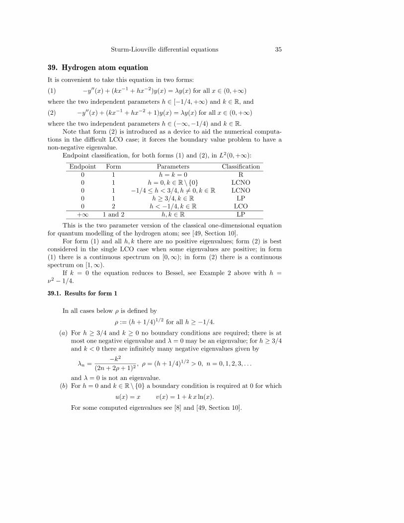
39. Hydrogen atom equation
It is convenient to take this equation in two forms:
(1) −y′′(x) + (kx−1 + hx−2)y(x) = λy(x) for all x ∈ (0,+∞)
where the two independent parameters h ∈ [−1/4,+∞) and k ∈ R, and
(2) −y′′(x) + (kx−1 + hx−2 + 1)y(x) = λy(x) for all x ∈ (0,+∞)
where the two independent parameters h ∈ (−∞,−1/4) and k ∈ R.Note that form (2) is introduced as a device to aid the numerical computa-
tions in the difficult LCO case; it forces the boundary value problem to have anon-negative eigenvalue.
Endpoint classification, for both forms (1) and (2), in L2(0,+∞):
Endpoint Form Parameters Classification0 1 h = k = 0 R0 1 h = 0, k ∈ R \ {0} LCNO0 1 −1/4 ≤ h < 3/4, h 6= 0, k ∈ R LCNO0 1 h ≥ 3/4, k ∈ R LP0 2 h < −1/4, k ∈ R LCO
+∞ 1 and 2 h, k ∈ R LP
This is the two parameter version of the classical one-dimensional equationfor quantum modelling of the hydrogen atom; see [49, Section 10].
For form (1) and all h, k there are no positive eigenvalues; form (2) is bestconsidered in the single LCO case when some eigenvalues are positive; in form(1) there is a continuous spectrum on [0,∞); in form (2) there is a continuousspectrum on [1,∞).
If k = 0 the equation reduces to Bessel, see Example 2 above with h =ν2 − 1/4.
39.1. Results for form 1
In all cases below ρ is defined by
ρ := (h+ 1/4)1/2 for all h ≥ −1/4.
(a) For h ≥ 3/4 and k ≥ 0 no boundary conditions are required; there is atmost one negative eigenvalue and λ = 0 may be an eigenvalue; for h ≥ 3/4and k < 0 there are infinitely many negative eigenvalues given by
λn =−k2
(2n+ 2ρ+ 1)2, ρ = (h+ 1/4)1/2 > 0, n = 0, 1, 2, 3, . . .
and λ = 0 is not an eigenvalue.(b) For h = 0 and k ∈ R \ {0} a boundary condition is required at 0 for which
u(x) = x v(x) = 1 + k x ln(x).
For some computed eigenvalues see [8] and [49, Section 10].
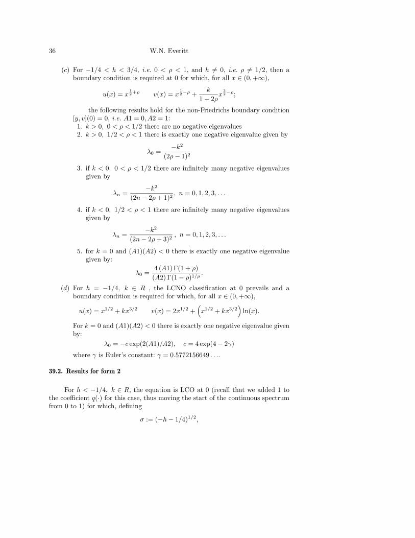
36 W.N. Everitt
(c) For −1/4 < h < 3/4, i.e. 0 < ρ < 1, and h 6= 0, i.e. ρ 6= 1/2, then aboundary condition is required at 0 for which, for all x ∈ (0,+∞),
u(x) = x12 +ρ v(x) = x
12−ρ +
k
1− 2ρx
32−ρ;
the following results hold for the non-Friedrichs boundary condition[y, v](0) = 0, i.e. A1 = 0, A2 = 1:
1. k > 0, 0 < ρ < 1/2 there are no negative eigenvalues2. k > 0, 1/2 < ρ < 1 there is exactly one negative eigenvalue given by
λ0 =−k2
(2ρ− 1)2
3. if k < 0, 0 < ρ < 1/2 there are infinitely many negative eigenvaluesgiven by
λn =−k2
(2n− 2ρ+ 1)2, n = 0, 1, 2, 3, . . .
4. if k < 0, 1/2 < ρ < 1 there are infinitely many negative eigenvaluesgiven by
λn =−k2
(2n− 2ρ+ 3)2, n = 0, 1, 2, 3, . . .
5. for k = 0 and (A1)(A2) < 0 there is exactly one negative eigenvaluegiven by:
λ0 =4 (A1) Γ(1 + ρ)
(A2) Γ(1− ρ)1/ρ.
(d) For h = −1/4, k ∈ R , the LCNO classification at 0 prevails and aboundary condition is required for which, for all x ∈ (0,+∞),
u(x) = x1/2 + kx3/2 v(x) = 2x1/2 +(x1/2 + kx3/2
)ln(x).
For k = 0 and (A1)(A2) < 0 there is exactly one negative eigenvalue givenby:
λ0 = −c exp(2(A1)/A2), c = 4 exp(4− 2γ)
where γ is Euler’s constant: γ = 0.5772156649 . . ..
39.2. Results for form 2
For h < −1/4, k ∈ R, the equation is LCO at 0 (recall that we added 1 tothe coefficient q(·) for this case, thus moving the start of the continuous spectrumfrom 0 to 1) for which, defining
σ := (−h− 1/4)1/2,

Sturm-Liouville differential equations 37
then, for all x ∈ (0,+∞),
u(x) = x1/2[(1− (4h)−1kx) cos(σ ln(x)) + kσx sin(σ ln(x))/2
]v(x) = x1/2
[(1− (4h)−1kx) sin(σ ln(x)) + kσx cos(σ ln(x))/2
];
(i) when k = 0 this equation reduces to the Krall equation Example 20 below(but note that the notation is different)
(ii) when k 6= 0 explicit formulas for the eigenvalues are not available; how-ever we report here on the qualitative properties of the spectrum for anyboundary condition at 0:
(α) for all k ∈ R there are infinitely many negative eigenvalues tend-ing exponentially to −∞
(β) for k > 0 there are only a finite number of eigenvalues in anybounded interval, in particular they do not accumulate at 1
(γ) for k ≤ 0 the eigenvalues accumulate also at 1.(δ) for k = 0 and (A1)(A2) < 0 there is exactly one negative eigen-
value given by:
λ0 =4 (A1) Γ(1 + ρ)
(A2) Γ(1− ρ)1/ρ.
Most of these results are due to Jorgens, see [49, Section 10]; a few new resultswere established by the authors of [11, Data base file xamples.tex; example 13].
40. Algebro-geometric equations
A potential q of the one-dimensional Schrodinger equation
L[y](x) := −y′′(x) + q(x)y(x) = λy(x) for all x ∈ I ⊆ R
is called an algebro-geometric potential if there exists a linear ordinary differentialexpression P of odd-order and leading coefficient 1, which commutes with L. Thereare deep relationships between algebro-geometric equations and the Korteweg-deVries hierarchy of non-linear differential equations. An overview of these propertiesand results can be found in the survey article [44] which contains a substantial listof references.
The main structure and properties of the algebro-geometric equations canonly be observed when the differential equations are considered in the complexplane, which would take the contents of this catalogue outside the environment ofthe Sturm-Liouville symmetric differential equations as given in Section 3 above.
However, three forms of algebro-geometric differential equations are givenhere; all three examples are Sturm-Liouville equations; two cases are related toother examples in this catalogue. However, all of these three examples have to beseen within the structure of algebro-geometric potentials and the relationships tonon-linear differential equations.

38 W.N. Everitt
40.1. Algebro-geometric form 1
Let l ∈ N0; then the differential equation is
−y′′(x) + l(l + 1)x−2y(x) = λy(x) for all x ∈ (0,∞).
this is a special case of:
(i) The hydrogen atom equation of Section 39 above, which gives the endpointclassification on (0,∞) for this example.
(ii) The Liouville form of the Bessel differential equation, see Section 12 above,when the parameter ν = l+1/2; these cases of Bessel functions are namedas the “spherical” Bessel functions; see [1, Chapter 10, Section 10.1] and[79, Chapter III, Section 3.41].
Endpoint classification in L2(0,+∞):
Endpoint Parameter Classification0 l = 0 R0 l ∈ N LP
+∞ l ∈ N0 LP
It is shown in [44] that this differential equation has two solutions of the form
y(x, λ) = exp (ixs)
sl +l∑
j=0
ajsl−j
xj
for all x ∈ (0,∞) and all λ ∈ C,
where:
(i) s2 := λ(ii) the coefficients {aj : j ∈ N0} are determined by
a0 = 1 and an+1 = il(l + 1)− n(n+ 1)
2(n+ 1)for all n ∈ N.
40.2. Algebro-geometric form 2
Let g ∈ N0; then the differential equation is
−y′′(x)− g(g + 1)cosh(x)2
y(x) = λy(x) for all x ∈ (−∞,∞);
this equation is a special case of:
(i) The hypergeometric differential equation, see Section 9 above but in par-ticular [78, Chapter IV, Section 4.19].
(ii) The Liouville form of the Jacobi function differential equation, see Section26 above, with the special case of α = −1/2 and β = g + 1/2; here, theinterval (0,∞) for the equation can be extended to (−∞,∞) since theorigin 0 is no longer a singular point of the equation when α = 1/2.
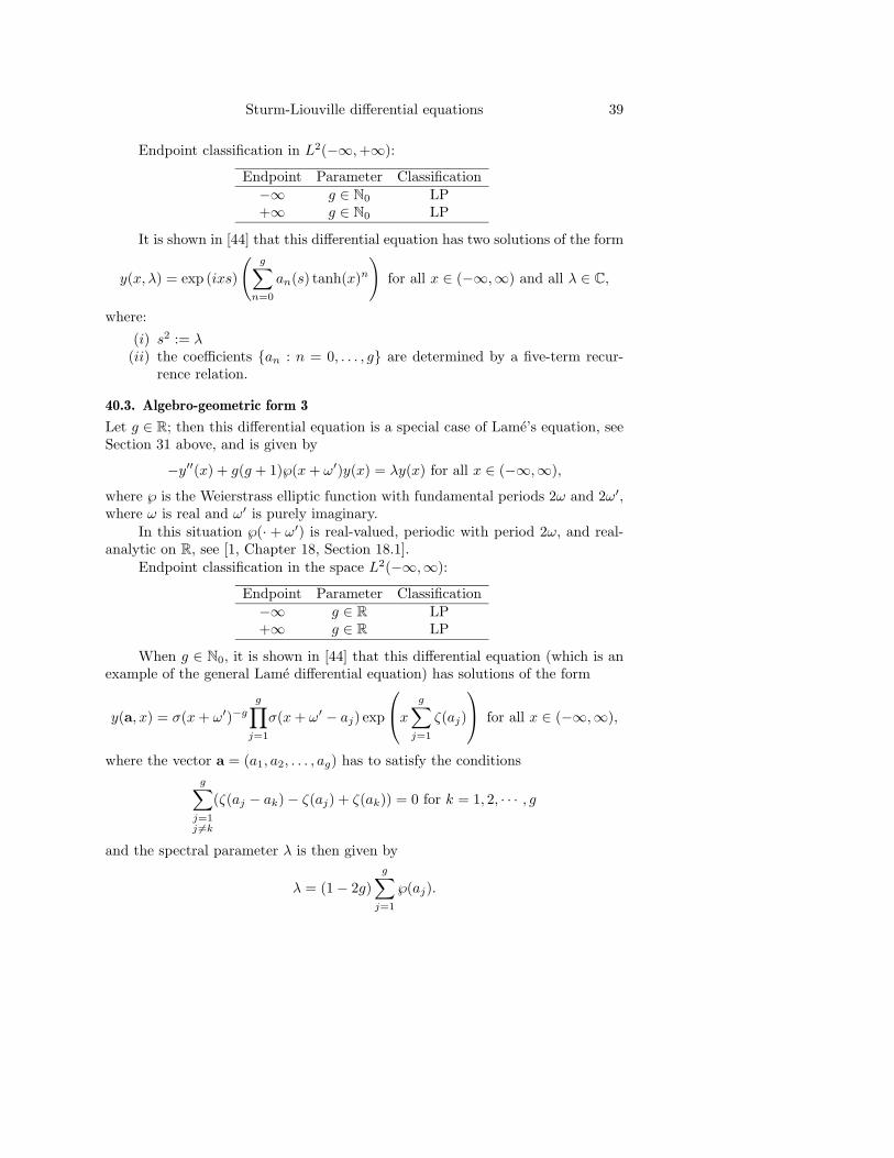
Sturm-Liouville differential equations 39
Endpoint classification in L2(−∞,+∞):
Endpoint Parameter Classification−∞ g ∈ N0 LP+∞ g ∈ N0 LP
It is shown in [44] that this differential equation has two solutions of the form
y(x, λ) = exp (ixs)
(g∑
n=0
an(s) tanh(x)n)
for all x ∈ (−∞,∞) and all λ ∈ C,
where:
(i) s2 := λ(ii) the coefficients {an : n = 0, . . . , g} are determined by a five-term recur-
rence relation.
40.3. Algebro-geometric form 3
Let g ∈ R; then this differential equation is a special case of Lame’s equation, seeSection 31 above, and is given by
−y′′(x) + g(g + 1)℘(x+ ω′)y(x) = λy(x) for all x ∈ (−∞,∞),
where ℘ is the Weierstrass elliptic function with fundamental periods 2ω and 2ω′,where ω is real and ω′ is purely imaginary.
In this situation ℘(· + ω′) is real-valued, periodic with period 2ω, and real-analytic on R, see [1, Chapter 18, Section 18.1].
Endpoint classification in the space L2(−∞,∞):
Endpoint Parameter Classification−∞ g ∈ R LP+∞ g ∈ R LP
When g ∈ N0, it is shown in [44] that this differential equation (which is anexample of the general Lame differential equation) has solutions of the form
y(a, x) = σ(x+ ω′)−gg∏j=1
σ(x+ ω′ − aj) exp
x g∑j=1
ζ(aj)
for all x ∈ (−∞,∞),
where the vector a = (a1, a2, . . . , ag) has to satisfy the conditionsg∑j=1j 6=k
(ζ(aj − ak)− ζ(aj) + ζ(ak)) = 0 for k = 1, 2, · · · , g
and the spectral parameter λ is then given by
λ = (1− 2g)g∑j=1
℘(aj).

40 W.N. Everitt
Here σ and ζ are the Weierstrass-σ and Weierstrass-ζ functions respectively, see[1, Chapter 18, Section 18.1].
The spectrum of the unique self-adjoint operator, in the Hilbert functionspace L2(−∞,∞), generated by this example of the Lame differential equation,consists of g+1 disjoint intervals, one of which is a semi-axis; these are the spectralbands of this differential operator.
Note that a satisfies the constraints mentioned if and only if −a satisfiesthe same constraint, since ζ is an odd function; as ℘ is an even function theseproperties lead to the same value of λ. Both the functions y(a, ·) and y(−a, ·) dothen satisfy the same differential equation; they are linearly independent exceptwhen λ is one of the 2g + 1 band edges.
For these results and additional examples of algebro-geometric differentialequations see the survey paper [44].
40.4. Algebro-geometric form 4
This form is named as the N -soliton potential.We introduce the N ×N matrix, for 1 ≤ j, k ≤ N and all x ∈ (−∞,∞),
CN (x) =(cjck(κj + κk)−1 exp(−(κj + κk)x
)with
cj > 0, κj > 0, κj 6= κk for all 1 ≤ j, k ≤ N with j 6= k;
the N -soliton potential qN : (−∞,∞)→ R is then defined by
qN (x) := −2d2
dx2ln(det(IN + CN (x))) for all x ∈ (−∞,∞)
(with IN the identity matrix in CN ). The corresponding Sturm-Liouville differen-tial equation then reads
−y′′(x) + qN (x)y(x) = λy(x) for all x ∈ (−∞,∞) and λ ∈ C.
SinceqN ∈ C∞(−∞,∞), qN (x) = O(exp(−2κj0 |x|)) for |x| → ∞,
where κj0 = min1≤j≤N (κj), where κ := max1≤j≤N (κj) for all x ∈ R.the endpointclassification in L2(−∞,∞) is
Endpoint Classification−∞ LP+∞ LP
Defining
cN,j,+ := cj , cN,j,− := c−1j ×
2κ1, j = N = 1,
2κjN∏k=1
κj + κkκj − κk
with k 6= j, 1 ≤ j ≤ N, N ≥ 2

Sturm-Liouville differential equations 41
two independent solutions of the differential equation, associated with qN , are thengiven by
fN,±(x, λ) :=
1− iN∑j=1
(√λ+ iκj)−1cN,j,±ψN,j(x) exp (∓κjx)
exp(±i√λx),
for all λ ∈ C with Im(√λ) ≥ 0, and all x ∈ (−∞,∞). Here {ψN,j(·) : j =
1, 2, . . . , N} are given as follows; define the column vector
Ψ0N (x) := (c1 exp(κ1x), . . . , cN exp(−κNx))>,
and then ΨN (·) by
ΨN (x) := [IN + CN (x)]−1ψ0N (x) for all x ∈ (−∞,∞),
both for all x ∈ (−∞,∞). Writing now
ΨN (x) = (ψN,1(x), . . . , ψN,N (x))>
this defines the components {ψN,j(·) : j = 1, 2, . . . , N} and completes the definitionof the two solutions fN,±.
Now let HN denote the (maximally defined) self-adjoint Schrodinger operatorwith potential qN in L2(−∞,∞). Then ψN,j ∈ C∞(−∞,∞) are exponentially de-caying eigenfunctions of HN as |x| → ∞, corresponding to the negative eigenvalues−κ2
j ; thusHNψN,j = −κ2
jψN,j , 1 ≤ j ≤ N.Moreover, HN has spectrum
{−κ2j : 1 ≤ j ≤ N} ∪ [0,∞)
and qN satisfies
qN (x) = −4N∑j=1
κjψN,j(x)2 < 0, 0 < −qN (x) ≤ 2κ2,
where κ := max1≤j≤N (κj) for all x ∈ R.The potentials qN are reflectionless since the corresponding 2× 2 scattering
matrix SN (λ) is of the form
SN (λ) =(TN (λ) RrN (λ)R`N (λ) TN (λ)
)for all λ ≥ 0,
with transmission coefficients given by
TN (λ) =N∏j=1
√λ+ iκj√λ− iκj
for all λ ≥ 0
and vanishing reflection coefficients from the right and left incidence
RrN (λ) = R`N (λ) = 0 for all λ ≥ 0.

42 W.N. Everitt
Thus, the N -soliton potentials qN can be thought of a particular constructionof reflectionless potentials that adds N negative eigenvalues −κ2
j , 1 ≤ j ≤ N , to thespectrum of H0, where H0 = −d2/dx2 is the Schrodinger operator in L2(−∞,∞)associated with the trivial potential q0(x) = 0 for all x ∈ R, and spectrum [0,∞).
It can be shown that qN satisfies a particular Nth stationary KdV equation,see [40, Section 1.3]. In addition, introducing an appropriate time-dependence incj leads to KdV N -soliton potentials, see [40, Section 1.4].
We also note that qg(x) = −g(g + 1)[cosh(x)]−2, treated in Subsection 40.2above, is a special case of qN for N = g and a particular choice of κj and cj ,1 ≤ j ≤ N .
Reflectionless potentials qN were first derived by Kay and Moses [51] (seealso [23], [24], [39], and [41] for detailed discussions).
41. Bargmann potentials
Let ϕ0(x, λ) = s−1 sin(sx) for λ = s2 ∈ C and x ∈ [0,∞); then for N ∈ N introducethe N ×N matrix
BN (x) = (BN,j,k(x)) for 1 ≤ j, k ≤ N and all x ∈ [0,∞)
given by
BN,j,k(x) =∫ x
0
Cjϕ0(t,−γ2j )ϕ0(t,−γ2
k) dt
= Cj(2γjγk)−1
(2γj)−1 sinh(2γjx)− x,for j = k,
(γj + γk)−1 sinh((γj + γk)x)− (γj − γk)−1 sinh((γj − γk)x),for j 6= k,
Cj > 0, γj > 0 for 1 ≤ j, k ≤ N.
Bargmann potentials qN are then defined by
qN (x) = −2d2
dx2ln(det(IN +BN (x))) for all x ∈ [0,∞)
(IN the identity matrix in CN ), and the associated Sturm-Liouville differentialequation reads
−y′′(x) + qN (x)y(x) = λy(x) for all x ∈ [0,∞) and λ ∈ C.
It can show that ∫ ∞0
(1 + x)|qN (x)| dx <∞.
Sturm-Liouville differential equations 43
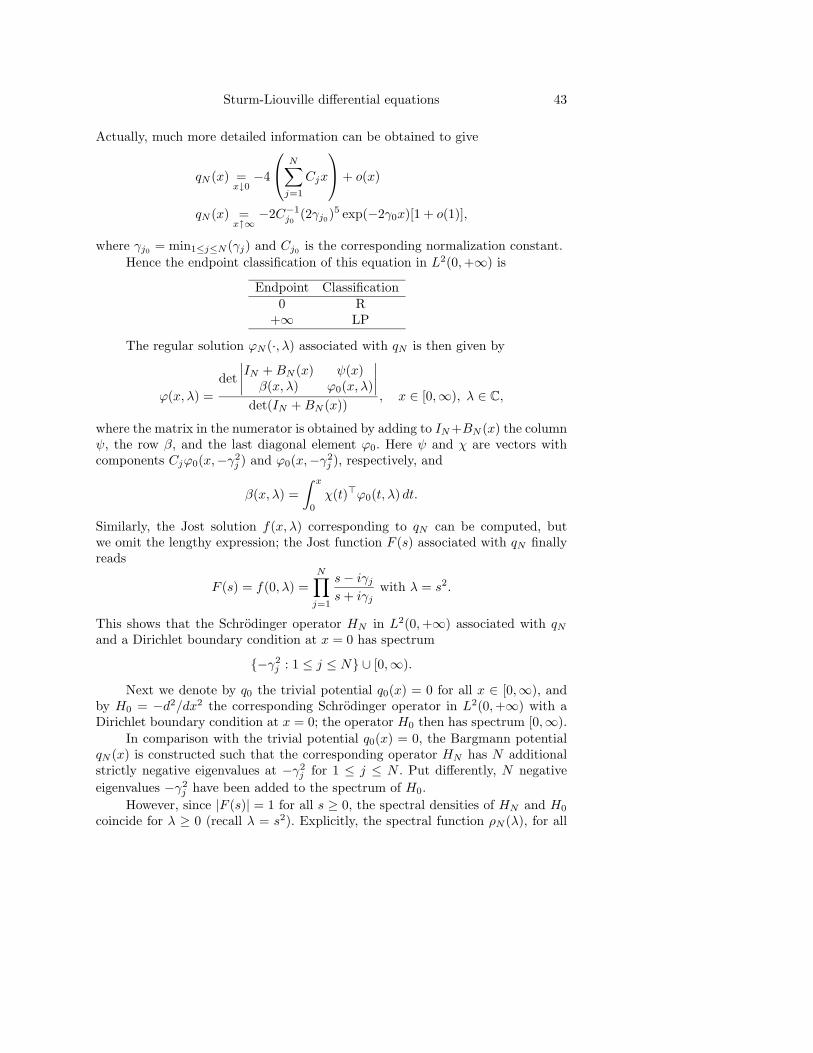
Actually, much more detailed information can be obtained to give
qN (x) =x↓0−4
N∑j=1
Cjx
+ o(x)
qN (x) =x↑∞−2C−1
j0(2γj0)5 exp(−2γ0x)[1 + o(1)],
where γj0 = min1≤j≤N (γj) and Cj0 is the corresponding normalization constant.Hence the endpoint classification of this equation in L2(0,+∞) is
Endpoint Classification0 R
+∞ LP
The regular solution ϕN (·, λ) associated with qN is then given by
ϕ(x, λ) =det∣∣∣∣IN +BN (x) ψ(x)
β(x, λ) ϕ0(x, λ)
∣∣∣∣det(IN +BN (x))
, x ∈ [0,∞), λ ∈ C,
where the matrix in the numerator is obtained by adding to IN+BN (x) the columnψ, the row β, and the last diagonal element ϕ0. Here ψ and χ are vectors withcomponents Cjϕ0(x,−γ2
j ) and ϕ0(x,−γ2j ), respectively, and
β(x, λ) =∫ x
0
χ(t)>ϕ0(t, λ) dt.
Similarly, the Jost solution f(x, λ) corresponding to qN can be computed, butwe omit the lengthy expression; the Jost function F (s) associated with qN finallyreads
F (s) = f(0, λ) =N∏j=1
s− iγjs+ iγj
with λ = s2.
This shows that the Schrodinger operator HN in L2(0,+∞) associated with qNand a Dirichlet boundary condition at x = 0 has spectrum
{−γ2j : 1 ≤ j ≤ N} ∪ [0,∞).
Next we denote by q0 the trivial potential q0(x) = 0 for all x ∈ [0,∞), andby H0 = −d2/dx2 the corresponding Schrodinger operator in L2(0,+∞) with aDirichlet boundary condition at x = 0; the operator H0 then has spectrum [0,∞).
In comparison with the trivial potential q0(x) = 0, the Bargmann potentialqN (x) is constructed such that the corresponding operator HN has N additionalstrictly negative eigenvalues at −γ2
j for 1 ≤ j ≤ N . Put differently, N negativeeigenvalues −γ2
j have been added to the spectrum of H0.However, since |F (s)| = 1 for all s ≥ 0, the spectral densities of HN and H0
coincide for λ ≥ 0 (recall λ = s2). Explicitly, the spectral function ρN (λ), for all
44 W.N. Everitt
λ ∈ (−∞,+∞), of HN is of the form
ρN (λ) =
{(2/3)π−1λ3/2, λ ≥ 0,∑Nj=1 Cjθ(λ+ γ2
j ), λ < 0
(here θ(t) = 1 for t > 0, θ(t) = 0 for t < 0), which should be compared with thespectral function ρ0(λ) of H0,
ρ0(λ) =
{(2/3)π−1λ3/2, λ ≥ 0,0, λ < 0.
For Bargmann’s original work we refer to [13], [14]; more details on Bargmannpotentials can be found in [21, Sections III.2, IV.1 and IV.3], and the referencestherein (see also [42, Section 11]).
42. Halvorsen equation
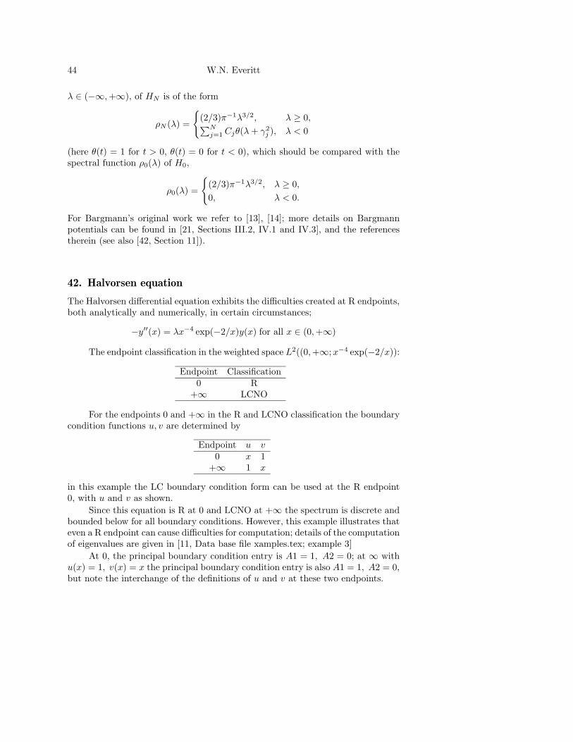
The Halvorsen differential equation exhibits the difficulties created at R endpoints,both analytically and numerically, in certain circumstances;
−y′′(x) = λx−4 exp(−2/x)y(x) for all x ∈ (0,+∞)
The endpoint classification in the weighted space L2((0,+∞;x−4 exp(−2/x)):
Endpoint Classification0 R
+∞ LCNO
For the endpoints 0 and +∞ in the R and LCNO classification the boundarycondition functions u, v are determined by
Endpoint u v0 x 1
+∞ 1 x
in this example the LC boundary condition form can be used at the R endpoint0, with u and v as shown.
Since this equation is R at 0 and LCNO at +∞ the spectrum is discrete andbounded below for all boundary conditions. However, this example illustrates thateven a R endpoint can cause difficulties for computation; details of the computationof eigenvalues are given in [11, Data base file xamples.tex; example 3]
At 0, the principal boundary condition entry is A1 = 1, A2 = 0; at ∞ withu(x) = 1, v(x) = x the principal boundary condition entry is also A1 = 1, A2 = 0,but note the interchange of the definitions of u and v at these two endpoints.

Sturm-Liouville differential equations 45
43. Jorgens equation
We have this example due to Jorgens [49];
−y′′(x) + (exp(2x)/4− k exp(x))y(x) = λy(x) for all x ∈ (−∞,+∞)
where the parameter k ∈ (−∞,+∞).Endpoint classification in the space L2(−∞,+∞), for all k ∈ (−∞,+∞):
Endpoint Classification−∞ LP+∞ LP
This is a remarkable example from Jorgens; numerical results are given in[11, Data base file xamples.tex; example 27]. Details of this problem are given in[49, Part II, Section 10]. For all k ∈ (−∞,+∞) the boundary value problem onthe interval (−∞,+∞) has a continuous spectrum on [0,+∞); for k ≤ 1/2 thereare no eigenvalues; for h = 0, 1, 2, 3, . . . and then k chosen by h < k− 1/2 ≤ h+ 1,there are exactly h+1 eigenvalues and these are all below the continuous spectrum;these eigenvalues are given explicitly by
λn = −(k − 1/2− n)2, n = 0, 1, 2, 3, . . . , h.
44. Rellich equation
The Rellich differential equation is, where the parameter K ∈ R,
−y′′(x) +Kx−2y(x) = λy(x) for all x ∈ (0,+∞);
this equation has a long and interesting history as indicated in the references, see[72], [65], [54], [20] and [43].
Here, we consider the equation in the form, where the parameter k ∈ (0,+∞),
−y′′(x) + (1− (k2 + 1/4)x−2)y(x) = λy(x) for all x ∈ (0,+∞)
as discussed in the paper [54], and in view of the connection with the computerprogram SLEIGN2, see [8] and [10].
Endpoint classification, for all k ∈ (0,+∞), in the space L2(0,+∞):
Endpoint Classification0 LCO
+∞ LP
This example should be seen as a special case of the Bessel Example 2 above;solutions can be obtained in terms of the modified Bessel functions.
To help with the computations for this example the spectrum is translatedby a term +1; this simple device is used for numerical convenience.
For problems with separated boundary conditions at endpoints 0 and ∞there is a continuous spectrum on [1,∞) with a discrete (and simple) spectrumon (−∞, 1). This discrete spectrum has cluster points at both −∞ and 1.

46 W.N. Everitt
For the LCO endpoint at 0 the boundary condition functions are given by
u(x) = x1/2 cos(k ln(x)) v(x) = x1/2 sin(k ln(x)).
For the boundary value problem on [0,∞) with boundary condition [y, u](0) =0 let the following conditions and notations apply:
(i) suppose Γ(1 + i) = α+ iβ and µ > 0 satisfies tan(ln(1
2µ))
= −α/β(ii) θ = Im(log(Γ(1 + i)))(iii) ln( 1
2µ) = 12π + θ + sπ for s = 0,±1,±2, ...
(iv) µ2s =
(2 exp(θ + 1
2π))2 exp(2sπ) s = 0,±1,±2, ...
then the eigenvalues are given explicitly by λn = −µ2−(n+1) +1 (n = 0,±1,±2, ...).
This problem creates major computational difficulties; see [11, Data basefile xamples.tex; example 20]. The program SLEIGN2 can compute only six ofthese eigenvalues in a normal UNIX server, even in double precision, specificallyλ−3 to λ2; other eigenvalues are, numerically, too close to 1 or too close to −∞.Here we list these SLEIGN2 computed eigenvalues in double precision in a normalUNIX server and compare them with the same eigenvalues computed from thetranscendental equation given above; for the problem on (0,∞) with k = 1 andA1 = 1.0, A2 = 0.0, the results are:
Eigenvalue eig from SLEIGN2 eig from trans. equ.−3 −276, 562.5 −14, 519, 130−2 −27, 114.48 −27, 114.67−1 −49.62697 −49.633180 0.9054452 0.90544541 0.9998234 0.99982342 0.9999997 0.9999997
45. Laplace tidal wave equation
This differential equation is given by:
−(x−1y′(x))′ +(kx−2 + k2x−1
)y(x) = λy(x) for all x ∈ (0,+∞),
where the parameter k ∈ (−∞, 0) ∪ (0,+∞). This equation has been studied bymany authors, in particular by Homer in his doctoral thesis [47] where a detailedlist of references is to be found:
Endpoint classification in L2(0,∞):
Endpoint Classification0 LCNO
+∞ LP
For the endpoint 0:
u(x) = x2 v(x) = x− k−1 for all x ∈ (0,+∞).
This equation is a particular case of the more general equation with thisname; for details and references see [47].

Sturm-Liouville differential equations 47
There are no representations for solutions of this differential equation in termsof the well-known special functions. Thus to determine boundary conditions at theLCNO endpoint 0 use has to be made of maximal domain functions; see the u, vfunctions given above. Numerical results for some boundary value problems andcertain values of the parameter k, are given in [11, Data base file xamples.tex;example 8].
46. Latzko equation
This differential equation is given by
−((1− x7)y′(x))′ = λx7y(x) for all x ∈ (0, 1].
Endpoint classification in L2(0, 1]:
Endpoint Classification0 R1 LCNO
For the endpoint 1:
u(x) = 1 v(x) = − ln(1− x) for all (0, 1).
This differential equation has a long and celebrated history; in particular ithas been studied by Fichera, see [36, Pages 43 to 45]. There is a LCNO singularityat the endpoint 1 which requires the use of maximal domain functions; see the u, vfunctions given above. The endpoint 0 is R but due to the fact that, in general,when a weight has the property w(0) = 0 then boundary value problems createdifficulties for numerical computations.
This example is similar in some respects to the Legendre equation of Section19 above.
For numerical results see [11, Data base file xamples.tex; example 7].
47. Littlewood-McLeod equation
This important example gives a Sturm-Liouville boundary value problem that hasa discrete spectrum that is unbounded above and below; the differential is
−y′′(x) + x sin(x)y(x) = λy(x) for all x ∈ [0,+∞).
Endpoint classification in the space L2(0,+∞):
Endpoint Classification0 R
+∞ LP
This differential equation is an example of the LPO endpoint classification intro-duced in [69, Chapter 7].
The spectral analysis of this differential equation is considered in [57] and[62]; the equation is R at 0 and LP at +∞. All self-adjoint operators in L2[0,∞)
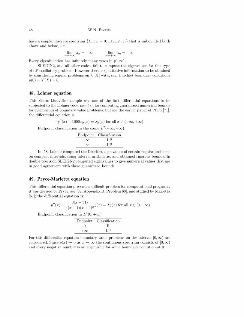
48 W.N. Everitt
have a simple, discrete spectrum {λn : n = 0,±1,±2, . . .} that is unbounded bothabove and below, i.e.
limn→−∞
λn = −∞ limn→+∞
λn = +∞.
Every eigenfunction has infinitely many zeros in (0,∞).SLEIGN2, and all other codes, fail to compute the eigenvalues for this type
of LP oscillatory problem. However there is qualitative information to be obtainedby considering regular problems on [0, X] with, say, Dirichlet boundary conditionsy(0) = Y (X) = 0.
48. Lohner equation
This Sturm-Liouville example was one of the first differential equations to besubjected to the Lohner code, see [58], for computing guaranteed numerical boundsfor eigenvalues of boundary value problems, but see the earlier paper of Plum [71];the differential equation is
−y′′(x)− 1000xy(x) = λy(x) for all x ∈ (−∞,+∞).
Endpoint classification in the space L2(−∞,+∞):
Endpoint Classification−∞ LP+∞ LP
In [58] Lohner computed the Dirichlet eigenvalues of certain regular problemson compact intervals, using interval arithmetic, and obtained rigorous bounds. Indouble precision SLEIGN2 computed eigenvalues to give numerical values that arein good agreement with these guaranteed bounds.
49. Pryce-Marletta equation
This differential equation presents a difficult problem for computational programs;it was devised by Pryce, see [69, Appendix B, Problem 60], and studied by Marletta[61]; the differential equation is:
−y′′(x) +3(x− 31)
4(x+ 1)(x+ 4)2y(x) = λy(x) for all x ∈ [0,+∞).
Endpoint classification in L2(0,+∞):
Endpoint Classification0 R
+∞ LP
For this differential equation boundary value problems on the interval [0,∞) areconsidered. Since q(x) → 0 as x → ∞ the continuous spectrum consists of [0,∞)and every negative number is an eigenvalue for some boundary condition at 0.
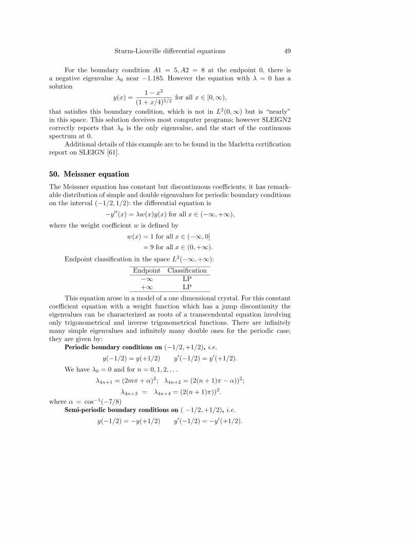
Sturm-Liouville differential equations 49
For the boundary condition A1 = 5, A2 = 8 at the endpoint 0, there isa negative eigenvalue λ0 near −1.185. However the equation with λ = 0 has asolution
y(x) =1− x2
(1 + x/4)5/2for all x ∈ [0,∞),
that satisfies this boundary condition, which is not in L2(0,∞) but is “nearly”in this space. This solution deceives most computer programs; however SLEIGN2correctly reports that λ0 is the only eigenvalue, and the start of the continuousspectrum at 0.
Additional details of this example are to be found in the Marletta certificationreport on SLEIGN [61].
50. Meissner equation
The Meissner equation has constant but discontinuous coefficients; it has remark-able distribution of simple and double eigenvalues for periodic boundary conditionson the interval (−1/2, 1/2): the differential equation is
−y′′(x) = λw(x)y(x) for all x ∈ (−∞,+∞),
where the weight coefficient w is defined by
w(x) = 1 for all x ∈ (−∞, 0]
= 9 for all x ∈ (0,+∞).
Endpoint classification in the space L2(−∞,+∞):
Endpoint Classification−∞ LP+∞ LP
This equation arose in a model of a one dimensional crystal. For this constantcoefficient equation with a weight function which has a jump discontinuity theeigenvalues can be characterized as roots of a transcendental equation involvingonly trigonometrical and inverse trigonometrical functions. There are infinitelymany simple eigenvalues and infinitely many double ones for the periodic case;they are given by:
Periodic boundary conditions on (−1/2,+1/2), i.e.
y(−1/2) = y(+1/2) y′(−1/2) = y′(+1/2).
We have λ0 = 0 and for n = 0, 1, 2, . . .
λ4n+1 = (2mπ + α)2; λ4n+2 = (2(n+ 1)π − α))2;
λ4n+3 = λ4n+4 = (2(n+ 1)π))2.
where α = cos−1(−7/8)Semi-periodic boundary conditions on ( −1/2,+1/2), i.e.
y(−1/2) = −y(+1/2) y′(−1/2) = −y′(+1/2).

50 W.N. Everitt
With β = cos−1((1 +√
(33))/16) and γ = cos−1((1 −√
(33))/16) these areall simple and given by, for n = 0, 1, 2, . . .
λ4n = (2nπ + β)2; λ4n+1 = (2nπ + γ)2;
λ4n+2 = (2(n+ 1)π − γ)2; λ4n+3 = (2(n+ 1)π − β)2.
For the general theory of periodic differential boundary value problems see [26];for a special case with discontinuous coefficients see [45].
51. Morse equation
This differential equation has exponentially small and large coefficients; the differ-ential equation is
−y′′(x) + (9 exp(−2x)− 18 exp(−x))y(x) = λy(x) for all x ∈ (−∞,+∞).
Endpoint classification in the space L2(−∞,+∞):
Endpoint Classification−∞ LP+∞ LP
This differential equation on the interval (−∞,∞) is studied in [5, Example6]; the spectrum has exactly three negative, simple eigenvalues, and a continuousspectrum on [0,∞); the eigenvalues are given explicitly by
λn = −(n− 2.5)2 for n = 0, 1, 2.
52. Morse rotation equation
This differential equation is considered in [5] and is given as
−y′′(x) + (2x−2 − 2000(2e(x)− e(x)2))y(x) = λy(x) for all x ∈ (0,+∞),
wheree(x) = exp(−1.7(x− 1.3)) for all x ∈ (0,+∞).
Endpoint classification in the space L2(0,+∞)
Endpoint Classification0 LP
+∞ LP
This classical problem on the interval (0,∞) has a continuous spectrum on[0,∞) and exactly 26 negative eigenvalues; it provides an invaluable numerical testfor computer programs.

Sturm-Liouville differential equations 51
53. Brusencev/Rofe-Beketov equations
53.1. Example 1
The Sturm-Liouville differential equation
−(x4y′(x))′ − 2x2y(x) = λy(x) for all x ∈ (0,∞)
is considered in the paper [19]; this example provides a LC case with specialproperties.
Endpoint classification in L2(0,+∞):
Endpoint Classification0 LP
+∞ LCNO
For the endpoint +∞ in the LCNO classification the boundary conditionfunctions u, v are determined by
Endpoint u v+∞ x−1 x−2
53.2. Example 2
The Sturm-Liouville differential equation
−y′′(x)−(x10 + x4sign(sin(x))
)y(x) = λy(x) for all x ∈ [0,∞)
is considered in the paper [73]; this example provides a LC case with specialproperties.
Endpoint classification in L2(0,+∞):
Endpoint Classification0 R
+∞ LCO
For the endpoint +∞ in the LCO classification the boundary condition func-tions u, v may be determined as the real and imaginary parts of the expression
x−5/2 exp(ix6/6)Y (x) for all x ∈ [1,∞),
where the function Y (·) is the solution of the integral equation, for x ∈ [1,∞),
Y (x) = 1 +i
2
∫ ∞x
(t−1sign(sin(t)) +
354t−7
)[exp
(i
3(t6 − x6)
)− 1]Y (t) dt.
The solution Y (·) of this integral equation may be obtained by the iteration methodof successive approximations; in this process it has to be noted that the integralsconcerned are only conditionally convergent.

52 W.N. Everitt
54. Slavyanov equations
In the important text [77] the authors give a systematic presentation of a unifiedtheory of special functions based on singularities of linear ordinary differentialequations in the complex plane C. In particular, in [77, Chapter 3], there is tobe found an authoritative account of the definition and properties of the Heundifferential equation.
In [77, Chapter 4] there is a chapter devoted to physical applications, in-cluding the use of the Heun differential equation, resulting from the applicationof separation techniques to boundary value problems for linear partial differentialequations. From this chapter we have selected three examples of Sturm-Liouvilledifferential equations; each equation contains a number of symbols denoting phys-ical constants and parameters which are given here without explanation. To allowthe quoted examples to be given in Sturm-Liouville form the notation for oneof these parameters has been changed to play the role of the spectral parameterλ ∈ C.
The resulting Sturm-Liouville examples given below have not yet been con-sidered for their endpoint classification, nor for their boundary condition functionsif required for LC endpoints.
54.1. Example 1
The hydrogen-molecule ion problem, see [77, Chapter 4, Section 4.1.3], gives thetwo differential equations:
−((1− η2)Y ′(η)
)′+(n2(1− η2)−1 − µ
)Y (η) = λη2Y (η) for all η ∈ (−1, 1)
and
−((1− ξ2)X ′(ξ)
)′+(κξ + n2(1− ξ2)− µ
)X(ξ) = λξ2X(ξ) for all ξ ∈ (1,∞).
54.2. Example 2
The Teukolsky equations in astrophysics gives the equation, see [77, Chapter 4,Section 4.2.1]:
−((1− u2)X ′(u))′ +(2 + (m− 2u)2(1− u2)−1 − 4aωu− a2ω2u2
)X(u) = λX(u)
for all u ∈ (−1, 1).
54.3. Example 3
The theory of tunneling in double-well potentials, see [77, Chapter 4, Section 4.4],gives the differential equation
−y′′(x) + V (x)y(x) = λy(x) for all x ∈ (−∞,∞)
with the potential V determined by
V (x) = −A(sech2(x+ x0) + sech2(x− x0)) for all x ∈ (−∞,∞);
here A is a number and x0 is a parameter.
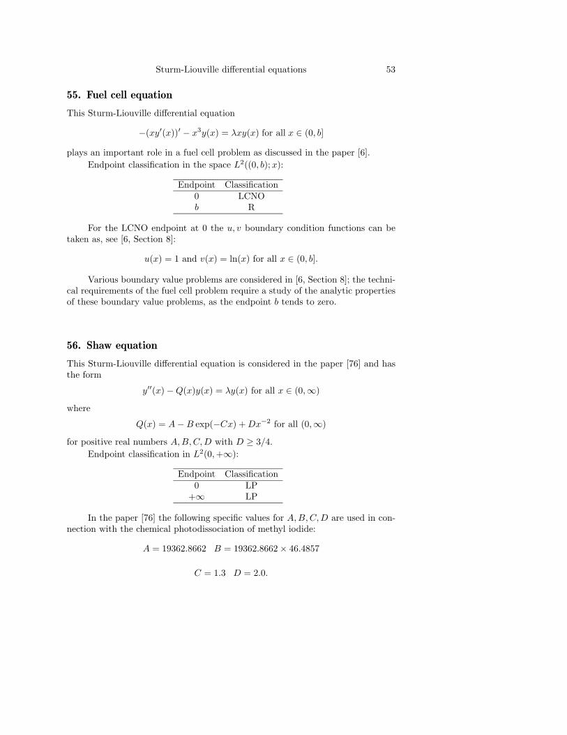
Sturm-Liouville differential equations 53
55. Fuel cell equation
This Sturm-Liouville differential equation
−(xy′(x))′ − x3y(x) = λxy(x) for all x ∈ (0, b]
plays an important role in a fuel cell problem as discussed in the paper [6].Endpoint classification in the space L2((0, b);x):
Endpoint Classification0 LCNOb R
For the LCNO endpoint at 0 the u, v boundary condition functions can betaken as, see [6, Section 8]:
u(x) = 1 and v(x) = ln(x) for all x ∈ (0, b].
Various boundary value problems are considered in [6, Section 8]; the techni-cal requirements of the fuel cell problem require a study of the analytic propertiesof these boundary value problems, as the endpoint b tends to zero.
56. Shaw equation
This Sturm-Liouville differential equation is considered in the paper [76] and hasthe form
y′′(x)−Q(x)y(x) = λy(x) for all x ∈ (0,∞)
where
Q(x) = A−B exp(−Cx) +Dx−2 for all (0,∞)
for positive real numbers A,B,C,D with D ≥ 3/4.Endpoint classification in L2(0,+∞):
Endpoint Classification0 LP
+∞ LP
In the paper [76] the following specific values for A,B,C,D are used in con-nection with the chemical photodissociation of methyl iodide:
A = 19362.8662 B = 19362.8662× 46.4857
C = 1.3 D = 2.0.

54 W.N. Everitt
57. Plum equation
This Sturm-Liouville equation is one of the first to be considered for numericalcomputation using interval arithmetic: the equation is
−(y′(x))′ + 100 cos2(x)y(x) = λy(x) for all x ∈ (−∞,+∞).
Endpoint classification in L2(−∞,+∞):
Endpoint Classification−∞ LP+∞ LP
In [71] the first seven eigenvalues for periodic eigenvalues on the interval[0, π],i.e.
y(0) = y(π) y′(0) = y′(π),are computed using a numerical homotopy method together with interval arith-metic; rigorous bounds for these seven eigenvalues are obtained.
58. Sears-Titchmarsh equation
This differential equation is considered in detail in [78, Chapter IV, Section 4.14]and [75]; the equation is
−y′′(x)− exp(2x)y(x) = λy(x) for all x ∈ (−∞,∞)
and has solutions of the form, using the Bessel function Jν and writing√λ = s =
σ + it,
y(x, λ) = Jis(exp(x)) for all x ∈ (−∞,∞);in the space L2(−∞,∞) this equation is LP at −∞ and is LCO at +∞. Thisdifferential equation is then another example of equations derived from the originalBessel differential equation.
This Sears-Titchmarsh differential equation is the Liouville form, see Section7 above, of the Sturm-Liouville equation
−(xy′(x))′ − xy(x) = λx−1y(x) for all x ∈ (0,+∞).
In the space L2((0,∞);x−1) this differential equation is LP at 0 and is LCO at+∞.
Endpoint classification in L2((0,∞);x−1):
Endpoint Classification0 LP
+∞ LCO
For the LCO endpoint +∞ the boundary condition functions can be chosenas, for all x ∈ (0,+∞),
u(x) = x−1/2 (cos(x) + sin(x)) v(x) = x−1/2 (cos(x)− sin(x)) .

Sturm-Liouville differential equations 55
For details of boundary value problems for this Sturm-Liouville equation,on [1,∞) see [8, Example 4]. For problems on [1,∞) the spectrum is simple anddiscrete but unbounded both above and below, since the endpoint +∞ is LCO.
Numerical results are given in [11, Data base file xamples.tex; example 6].
59. Zettl equation
This differential equation is closely linked to the classical Fourier equation 8;
−(x1/2y′(x))′ = λx−1/2y(x) for all x ∈ (0,+∞).
Endpoint classification in L2(0,+∞)
Endpoint Classification0 R
+∞ LP
This is a devised example to illustrate the computational difficulties of reg-ular problems which have mild (integrable) singularities, in this example at theendpoint 0 of (0,∞).
The differential equation gives p(0) = 0 and w(0) =∞ but nevertheless 0 isa regular endpoint in the Lebesgue integral sense; however this endpoint 0 doesgive difficulties in the in the computational sense.
The Liouville normal form of this equation is the Fourier equation, see Section8 above; thus numerical results for this problem can be checked against numericalresults from (i) a R problem, (ii) the roots of trigonometrical equations, and (iii)as a LCNO problem (see below).
There are explicit solutions of this equation given by
cos(2x1/2√λ) ; sin(2x1/2√λ)/√λ.
If 0 is treated as a LCNO endpoint then u, v boundary condition functionsare
u(x) = 2x1/2 v(x) = 1.
The regular Dirichlet condition y(0) = 0 is equivalent to the singular con-dition [y, u](0) = 0. Similarly the regular Neumann condition (py′)(0) = 0 isequivalent to the singular condition [y, v](0) = 0.
The following indicated boundary value problems have the given explicitformulae for the eigenvalues:
y(0) = 0 or [y, u](0) = 0, and y(1) = 0 gives
λn = ((n+ 1)π)2/4 (n = 0, 1, ...)
(py′)(0) = 0 or [y, v](0) = 0, and (py′)(1) = 0 gives
λn =((n+ 1
2 )π)2/4 (n = 0, 1, ...).
56 W.N. Everitt
60. Remarks
1. The author has made use of an earlier collection of examples of Sturm-Liouville differential equations drawn up by Bailey, Everitt and Zettl, inconnection with the development and testing of the computer programSLEIGN2; see [8] and [10].
2. The author has made use of major collections of Sturm-Liouville differen-tial equations from Pryce [69] and [70], and from Fulton, Pruess and Xie[38] and [68].
3. This catalogue will continue to be developed; the author welcomes correc-tions to the present form, and information about additional examples toextend the scope, of the catalogue.
61. Acknowledgments
1. The author is grateful to Werner Amrein (University of Geneva, Switzer-land), David Pearson (University of Hull, England, UK) and other col-leagues who organized the Sturm meeting, held at the University of Genevain September 2003, which brought together so many scientists working inand making application of Sturm-Liouville theory.
2. The author is grateful to many colleagues who commented on the earlierdrafts and sent information concerning possible examples to include in thiscatalogue: Werner Amrein, Paul Bailey, Richard Cooper, Desmond Evans,Charles Fulton, Fritz Gesztesy, Don Hinton, Hubert Kalf, Lance Little-john, Clemens Markett, Marco Marletta, Lawrence Markus, David Pear-son, Michael Plum, John Pryce, Fiodor Rofe-Beketov, Ken Shaw, BarrySimon, Sergei Slavyanov, Rudi Weikard, Tony Zettl.
3. The author is especially indebted to Barry Simon, Fritz Gesztesy, ClemensMarkett, John Pryce, Fiodor Rofe-Beketov and Rudi Weikard who sup-plied detailed information for the examples in Sections 11, 24, 25, 26, 31,40, 41, 49 and 53.
62. The future
As mentioned above it is hoped to continue this catalogue as a database for Sturm-Liouville differential equations.
The main contributor to the assessment and extension of successive draftsof this catalogue is Fritz Gesztesy, who has agreed to join with the author incontinuing to update the content of this database.
Together we ask that all proposals for enhancing and extending the cataloguebe sent to both of us, if possible by e-mail and LaTeX file. The author’s affiliationdata is to be found at the end of this paper; the corresponding data for FritzGesztesy is:

Sturm-Liouville differential equations 57
Fritz GesztesyDepartment of Mathematics
University of MissouriColumbia, MO 65211
USAe-mail: [email protected]
fax: ++ 1 573 882 1869
References
[1] M. Abramowitz and I.A. Stegun, Handbook of mathematical functions, Dover Publi-cations, Inc., New York, 1972.
[2] N.I. Akhiezer and I.M. Glazmann, Theory of linear operators in Hilbert space: I andII, Pitman and Scottish Academic Press, London and Edinburgh, 1981.
[3] R.A. Askey, T.H. Koornwinder and W. Schempp, Editors of Special functions: grouptheoretical aspects and applications, D. Reidel Publishing Co., Dordrecht, 1984.
[4] F.V. Atkinson, W.N. Everitt and A. Zettl, Regularization of a Sturm-Liouville prob-lem with an interior singularity using quasi-derivatives, Diff. and Int. Equations 1(1988), 213-222.
[5] P.B. Bailey, SLEIGN : An eigenvalue-eigenfunction code for Sturm-Liouville prob-lems, Report Sand77-2044, Sandia National Laboratory, New Mexico, USA: 1978.
[6] P.B. Bailey, J. Billingham, R.J. Cooper, W.N. Everitt, A.C. King, Q. Kong, H. Wuand A. Zettl, Eigenvalue problems in fuel cell dynamics, Proc. Roy. Soc. London (A)459 (2003), 241-261.
[7] P.B. Bailey, W.N. Everitt, D.B. Hinton and A. Zettl, Some spectral properties of theHeun differential equation. Operator Theory: Advances and Applications 132 (2002),87-110.
[8] P.B. Bailey, W.N. Everitt and A. Zettl, Computing eigenvalues of singular Sturm-Liouville problems, Results in Mathematics, 20 (1991), 391-423.
[9] P.B. Bailey, W.N. Everitt and A. Zettl, Regular and singular Sturm-Liouville prob-lems with coupled boundary conditions, Proc. Royal Soc. Edinburgh (A) 126 (1996),505-514.
[10] P.B. Bailey, W.N. Everitt and A. Zettl, The SLEIGN2 Sturm-Liouville code, ACMTrans. Math. Software. 27 (2001), 143-192. This paper may also be downloaded asthe LaTeX file bailey.tex from the web site: http://www.math.niu.edu/˜zettl/SL2
[11] P.B. Bailey, W.N. Everitt and A. Zettl, The SLEIGN2 database; Web site:http://www.math.niu.edu/˜zettl/SL2
[12] P.B. Bailey, W.N. Everitt, J. Weidmann and A. Zettl, Regular approximation ofsingular Sturm-Liouville problems, Results in Mathematics 23 (1993), 3-22.
[13] V. Bargmann, Remarks on the determination of a central field of force from theelastic scattering phase shifts, Phys. Rev. 75 (1949), 301-303.
[14] V. Bargmann, On the connection between phase shifts and scattering potential, Rev.Mod. Phys. 21 (1949), 488-493.
58 W.N. Everitt
[15] H. Behnke and F. Goerisch, Inclusions for eigenvalues of self-adjoint problems, J.Herzberger (Hrsg.): Topics in Validated Computation, North Holland Elsevier, Am-sterdam, (1994).
[16] W.W. Bell, Special functions for scientists and engineers, Van Nostrand, London,1968.
[17] G. Birkhoff and G-C. Rota, Ordinary differential equations, Wiley, New York, 1989.
[18] J.P. Boyd, Sturm-Liouville eigenvalue problems with an interior pole, J. Math.Physics, 22 (1981), 1575-1590.
[19] A.G. Brusencev and F.S. Rofe-Beketov, Conditions for the selfadjointness of stronglyelliptic systems of arbitrary order, Mt. Sb. (N.S.) 95 (137) (1974), 108-129, 160.
[20] W. Bulla and F. Gesztesy, Deficiency indices and singular boundary conditions inquantum mechanics, J. Math. Phys. 26 (1985), 2520-2528.
[21] K. Chadan and P.C. Sabatier, Inverse Problems in Quantum Scattering Theory, 2nded., Springer-Verlag, New York, 1989.
[22] E.T. Copson, Theory of functions of a complex variable, Oxford University Press,Oxford, 1946.
[23] P.A. Deift, Applications of a commutation formula. Duke Math. J. 45 (1978), 267-310.
[24] P. Deift and E. Trubowitz, Inverse scattering on the line. Comm. Pure Appl. Math.32 (1979), 121-251.
[25] N. Dunford and J.T. Schwartz, Linear Operators, part II, Interscience Publishers,New York, 1963.
[26] M.S.P. Eastham, The spectral theory of periodic differential equations, Scottish Aca-demic Press, Edinburgh and London, 1973.
[27] A. Erdelyi, Higher transcendental functions: I, II and III, McGraw-Hill, New York,1953.
[28] W. D. Evans and W.N. Everitt, On an inequality of Hardy-Littlewood type: I., Proc.Royal Soc. Edinburgh (A) 101 (1985), 131–140.
[29] W.D. Evans, W.N. Everitt, W.K. Hayman and D.S. Jones, Five integral inequalities:an inheritance from Hardy and Littlewood, Journal of Inequalities and Applications2 (1998), 1-36.
[30] W.N. Everitt, On the transformation theory of ordinary second-order linear sym-metric differential equations, Czechoslovak Mathematical Journal 32 (107) (1982),275–306.
[31] W.N. Everitt, J. Gunson and A. Zettl, Some comments on Sturm-Liouville eigenvalueproblems with interior singularities, J. Appl. Math. Phys. (ZAMP) 38 (1987), 813-838.
[32] W.N. Everitt and D.S. Jones, On an integral inequality, Proc. Royal Soc. London(A) 357 (1977), 271–288.
[33] W.N. Everitt and C. Markett, On a generalization of Bessel functions satisfyinghigher-order differential equations, Jour. Comp. Appl. Math. 54 (1994), 325-349.
[34] W.N. Everitt and L. Markus, Boundary value problems and symplectic algebra forordinary and quasi-differential operators, Mathematical Surveys and Monographs,61, American Mathematical Society, RI, USA, 1999.

Sturm-Liouville differential equations 59
[35] W.N. Everitt and A. Zettl, On a class of integral inequalities, J. London Math. Soc.(2) 17 (1978), 291–303.
[36] G. Fichera, Numerical and quantitative analysis, Pitman Press, London, 1978.
[37] M. Flendsted-Jensen and T. Koornwinder, The convolution structure for Jacobi func-tion expansions, Ark. Mat. 11 (1973), 245-262.
[38] C.T. Fulton and S. Pruess, ‘Mathematical software for Sturm-Liouville problems.’NSF Final Report for Grants DMS88 and DMS88-00839, 1993.
[39] C.S. Gardner, J.M. Greene, M.D. Kruskal, and R.M. Miura, Korteweg-deVries equa-tion and generalizations. VI. Methods for exact solution, Comm. Pure Appl. Math.27 (1974), 97-133.
[40] F. Gesztesy and H. Holden, Soliton equations and their algebro-geometric solutions.Vol. I: (1+1)-dimensional continuous models, Cambridge Studies in Advanced Math-ematics, Vol. 79, Cambridge University Press, 2003.
[41] F. Gesztesy, W. Karwowski and Z. Zhao, Limits of soliton solutions, Duke Math. J.68 (1992), 101-150.
[42] F. Gesztesy and B. Simon, A new approach to inverse spectral theory, II. Generalreal potentials and the connection to the spectral measure, Ann. Math. 152 (2000),593-643
[43] F. Gesztesy and M. Unal, Perturbative oscillation criteria and Hardy-type inequali-ties, Math. Nach. 189 (1998), 121-144.
[44] F. Gesztesy and R. Weikard, Elliptic algebro-geometric solutions of the KdV andAKNS hierarchies - an analytic approach, Bull. Amer. Math. Soc. 35 (1998), 271-317.
[45] H. Hochstadt, A special Hill’s equation with discontinuous coefficients, Amer. Math.Monthly, 70 (1963), 18-26.
[46] H. Hochstadt, The functions of mathematical physics, Wiley-Interscience, New York,1971.
[47] M.S. Homer, Boundary value problems for the Laplace tidal wave equation, Proc.Roy. Soc. of London (A) 428 (1990), 157-180.
[48] E.L. Ince, Ordinary differential equations, Dover, New York, 1956.
[49] K. Jorgens, Spectral theory of second-order ordinary differential operators, LectureNotes: Series no.2, Matematisk Institut, Aarhus Universitet, 1962/63.
[50] K. Jorgens and F. Rellich, Eigenwerttheorie gewohnlicher Differentialgleichungen,Springer-Verlag, Heidelberg, 1976.
[51] I. Kay and H.E. Moses, Reflectionless transmission through dielectrics and scatteringpotentials, J. Appl. Phys. 27 (1956), 1503-1508.
[52] E. Kamke, Differentialgleichungen: Losungsmethoden und Loungen: Gewonliche Dif-ferentialgleichungen, 3rd edition, Chelsea Publishing Company, New York, 1948.
[53] T.H. Koornwinder, Jacobi functions and analysis on noncompact semisimple Liegroups, Special functions: group theoretical aspects and applications, 1-85, D. ReidelPublishing Co., Dordrecht, 1984; Edited by R.A. Askey, T.H. Koornwinder and W.Schempp.
[54] A.M. Krall, Boundary value problems for an eigenvalue problem with a singularpotential, J. Diff. Equations, 45 (1982), 128-138.

60 W.N. Everitt
[55] W. Lay and S. Yu. Slavyanov, Heun’s equation with nearby singularities. Proc. R.Soc. Lond. A 455 (1999), 4374-4261.
[56] J. Liouville and J.C.F. Sturm, Extrait d’un memoire sur le developpement des func-tions en serie, Jour. Math. Pures et Appl. de Liouville II (1837), 220-223.
[57] J.E. Littlewood, On linear differential equations of the second order with a stronglyoscillating coefficient of y, J. London Math. Soc. 41 (1966), 627-638.
[58] R.J. Lohner, Verified solution of eigenvalue problems in ordinary differential equa-tions. (Personal communication, 1995.)
[59] J. Lutzen, Sturm and Liouville’s work on ordinary linear differential equations. Theemergence of Sturm-Liouville theory, Arch. Hist. Exact Sci. 29 (1984), 309-376.
[60] L. Markus and R.A. Moore, Oscillation and disconjugacy for linear differential equa-tions with almost periodic coefficients, Acta. Math. 96 (1956), 99-123.
[61] M. Marletta, Numerical tests of the SLEIGN software for Sturm-Liouville problems,ACM Trans. Math. Software. 17 (1991), 501-503.
[62] J.B. McLeod, Some examples of wildly oscillating potentials, J. London Math. Soc.43 (1968), 647-654.
[63] P.M. Morse, Diatomic molecules according to the wave mechanics: II: Vibration lev-els, Phys. Rev. 34 (1929), 57-61.
[64] M.A. Naimark, Linear differential operators: II, Ungar Publishing Company, NewYork, 1968.
[65] H. Narnhofer, Quantun theory for 1/r2-potentials, Acta Phys. Austriaca 40 (1974),306-322.
[66] H.-D. Niessen and A. Zettl, Singular Sturm-Liouville problems; the Friedrichs exten-sion and comparison of eigenvalues, Proc. London Math. Soc. 64 (1992), 545-578.
[67] E.G.P. Poole, Introduction to the theory of linear differential equations, Oxford Uni-versity Press, 1936.
[68] S. Pruess, C.T. Fulton and Y. Xie, Performance of the Sturm-Liouville softwarepackage SLEDGE, Technical Report MCS-91-19, Department of Mathematical andComputer Sciences, Colorado School of Mines, USA, 1994.
[69] J.D. Pryce, Numerical solution of Sturm-Liouville problems, Oxford University Press,1993.
[70] J.D. Pryce, A test package for Sturm-Liouville solvers, ACM Trans. Math. Software25 (1999), 21-57.
[71] M. Plum, Eigenvalue inclusions for second-order ordinary differential operators by anumerical homotopy method, ZAMP, 41 (1990), 205-226.
[72] F. Rellich, Die zulassigen Randbedingungen bei den singularen Eigenwertproblemender mathematischen Physik, (Gewohnliche Differentialgleichungen zweiter Ordnung),Math. Z. 49 (1944), 702–723.
[73] F.S. Rofe-Beketov, Non-semibounded differential operators. Teor. FunkciıFunkcional. Anal. i Prilozen. Vyp. 2 (1966), 178-184.
[74] A. Ronveaux, Heun differential equations, Oxford University Press, 1995.
[75] D.B. Sears and E.C. Titchmarsh, Some eigenfunction formulae, Quart. J. Math.Oxford (2) 1 (1950), 165-175.
Sturm-Liouville differential equations 61
[76] J.K. Shaw, A.P. Baronavski and H.D. Ladouceur, Applications of the Walker method,Spectral Theory and Computational Methods of Strum-Liouville problems: LectureNotes in Pure and Applied Mathematics 191 (1997), 377-395. (Marcel Dekker, Inc.,New York: 1997.)
[77] S. Yu. Slavyanov and W. Lay, Special functions: a unified theory based on singulari-ties, Oxford University Press, 2000.
[78] E.C. Titchmarsh, Eigenfunction expansions associated with second- order differentialequations: I, Clarendon Press, Oxford; 1962.
[79] G.N. Watson, A treatise on the theory of Bessel functions, Cambridge UniversityPress, Cambridge, England, 1958.
[80] E.T. Whittaker and G.N. Watson, Modern analysis, Cambridge University Press,1950.
[81] A. Zettl, Computing continuous spectrum, Proc. International Symposium, Trendsand Developments in Ordinary Differential Equations, Y. Alavi and P. Hsieh editors,World Scientific, (1994), 393-406.
[82] A. Zettl, Sturm-Liouville problems, Spectral Theory and Computational Methodsof Sturm-Liouville problems: Lecture Notes in Pure and Applied Mathematics 191(1997), 1-104. (Marcel Dekker, Inc., New York: 1997.)
W.N. Everitt, School of Mathematics and Statistics, University of Birmingham,Edgbaston, Birmingham B15 2TT, England, UKE-mail address: [email protected]