\

I'

I

L

A CASE STUDY ON

MOST OPTIMAL POWER FLOW SOLUTIONS

TO SUPPLY POWER TO A NEW RESIDENTIAL COMPOUND LOAD

LOCATED AT THE OUTSKIRTS OF AN INDUSTRIAL AREA BY USING THE } 7

OPTIMIZATION TOOLS

By

Nidal Abrahim Othman

Bachelor of Electrical Power Engineering, Jordan, 1994

The Project presented to

Ryerson University

in partial fulfillment of the requirements for the degree of

. ~ " Master of Engineering

or

in the Program of

Electrical and Computer Engineering (ECE)

Toronto, Ontario, Canada, 2011 .

© Nidal Abrahim Othman 2011

" ..... .: -, ~ ':-

I i °

!

f I

Author's Declaration:

I hereby declare that I am the sole author of this project.

.. ~ • T _ '", _ -" ..,.

I authorize Ryerson University to lend ~his project to other institutions or individuals for the

purpose of scholarly research.

Nidal Abrahim Othman

I further authorize Ryerson University to reproduce this project by photocopying or by other

meansl

in total or in part, at the request of other institutions or individuals for the purpose of

scholarly research.

. -

Nidal Abrahim Othman

(ii)

I Borrow list

Ryerson University requires the signatures of all persons using or photoc~pying this project.

Please sign below, and give address and date.

;.'

(iii)

- • if .• 11

j 11 . 'I , I

] -I ./ , 1

'J i 1

I i i

Acknowledgements

I would like to thank my advisor Dr. Kaamran Raahemifar for his continued guidance and

support through'out my Master's program. He ha's been a' g'reat me~tor, ~n'd an excellent'role

model in research.

I would also like to thank all of my family members and my friends from Ryerson

University for their support of me during my Master of Engineering program and project

preparation.

(iv)

I

t r

I

, I I

Abstract Nidal Abrahim Othman, M.Eng. ECE, Ryerson University, Toronto, 2011.

This project studies different solutions, presents an efficient and reliable approach, to solve

the optimal power flow (OPF) problem for an industrial power system by using fmincon

optimization method and technique. This fmincon toolbox from MATLAB attempts to find a . -

constrained minimum of a scalar function of several variables starting at an initial estimate. This

is generally referred to as constrained nonlinear optimization or nonlinear programming.

The objective in OPF problem is to minimize the total cost function of generating units and the

transmission losses, while maintaining the design and performance of the entire power system,

satisfying .~he opera~ional requirements such as the real and reactive power outputs of the

generating units, bus voltages and power flow of transmission lines ... etc.

This project presents the most optimal ~olution of power flow incorporating wind generation

cost, to supply power to a new domestic load located at the outskirts of an industrial area for i '

th~ee different scenarios. This residential is typical of long rural line with isolat,~d load area. 4 , ••

The challenge in our case study is to incorporate a wind generation unit as one type of green '. ~ 't,"

energy, that are currently being considered as an alternative source of power, to feed this long

Jural line for the domestic load without effecting in the total generation cost. " -~.,

A case study is carried out for three different scenarios incorporating wind generation cost. The .., .. Ir ,t -. "

results of OPF in this project shows that incorporating wind generation unit as renewable . , , ., ~,

energy source with the entire power system will have a minimum generation cost and .., . ~

minimum transmission losses for the entire power system even if the wind generation cost ~ 'i! ~~ ~.

assumed to, be the most expensive one comparing ~ith other conventional generation units.

This p'roject re'po'rt"provides 'implementation of Algorithm for the' ~~tire power I~;~ flow using .i • "<:.

~he ~ast decoupled power flow (FDPF) and optimizes the best solution for the three different

scenarios by using fmincon Interior Point Algorithm as one of optimization toolbox to achieve

the minimum total cost function of generating units and minimum transmission losses.

(v)

. , , ,

!

1 "

/.

I '

I

I ~ ! ~ , I r ~ ~ n

~ • ,I I:'

" ,

Table of Contents

1 INTRODUCTION ................................................................................................................... 1

2 OPF DESIGN CHALLENGES ................................................................................................... 2

3

4

5

'""". ~ ,

.' 2.1 . POWER SYSTEM STRUCTURE ................................................................................. 2

. 2.2 ElECTRICITY MARKET STRUCTURE & DISPATCHING PRACTICE ................ ; ......... ; ... 4

OPF SURVEyS· .................................. : .... : ..................... ·: ................................................ ~.~·: ... -....... 7

WIND GENERATION TECHNOLOGY IN OPF .. ~ ............................................... : .................... · .... 8

4.1- . GREEN ENERGY TYPES ....................... ; ...... : ... ~ ..................... : .................. : .................. 8

4.2 COST COMPARISONS OF GREEN ENERGY SUPPLYTECHNOlOGIES ................. ~ .... 9

THEORY OF OPTIMAL POWER FLOW (OPF) ................................................................... : ... 13

5.1 OPF PROBLEM .............. : .. : .............. ~ .. : ............................. ; .... : ... ~ •• : ...... ::;:: ... ; ... :~ ... ~ ... 13

5.2'

5.3

5.4

5.5

5.6

OPF SOLUTIONS & RESUlTS ............ : ...... : ............... : .. : •• ~ .... : .. ::: ........ :.:~ ..................... 13·

. - ',' ;

PROBLEM FORMULATION ................................................................................... 15

OBJECTIVE FUNCTION ........ : ................ ~: ......... :.' .................. ~: ........... ~.~ •••..•••..••• : .... 1S \ TYPES OF EQUALITY CONSTRAINTS ..... :: ............. : ................ : .......... ~ ...... :: ............... 16

. . TYPES OF INEQUALITY CONSTRAINTS ..................................................................... 16

6 . PROJECT CASEE STUDY USING OPF METHODOL<:JGY •• : ....... : ..... : .. ~.·:.:.: .... : ....... : ............. · ... 18 . -

6.1 DISCUSSION & THEORy ........................ :: .............................................................. 18 . ,~", "

, 6.2 PROJECT PROPOSAL (CASE STUDy) ...................................................................... 20 ,-6.3 ,. PROJECT RESULT ANALYSIS ................................................................................. 24

. ~."

7 CONSLUSION AND FUTURE WORK ...................................................................................... 26 V' • , i: < , :'., '~ f:' _ .... ".. , : ,:"

REFERENCES ...................................................................................................................... 28 .. • p', , - ~, ' . • '" -.... ",' i

APPEN Q.IX ............................... ! •••••••.••••..•••.••• ...................... !~ •••• ~ •••••••••• ~ •• ................. !& .............. :32

(vi)

I I

I l

list of Tables, Table 1: Cost Compa"risons of Energy Supply Technologies .......... ~ ......................................... 10

-" ~. '.. -

Table 2:, Test Results Analysis for Three Different Scenarios ................................................ 24

list of Figures Fig.1: H.V. Transmission lines Interconnection in Ontario Province .................................... 2

, )

Fig.2: Components of Power System ....................................................................................... 3

Fig.3: Base Loads in Typical Power System ............................................. ~.: .......................... 3'->

Fig.4: Electricity Market Structure .................................. : ...................................................... 4

~ " . -

Fig.S: Typical Offer for Market Structure ....................................... ~~ . .::, ...... ~ .. ; ............. ~ ..... ~~ ..... ; ... 5 . I

Fig.6: Total Capital Costs for different types of green energy ........................................ ; ... 11 . '

. . .

Fig.7: Operational Costs for different types of green energy ........................................... :. 11

, Fig.S: Net Yearly Cost (life/C~pital}inclt.iding the Yearly Running Cost ............................... 12 : ..- -.,-.- -'~~"----' ... ~

'"

Fig.9: Power Production Cost ($/KWH) for different types of energy ... ~~ •.. ~ ......... '.~ .............. 12 /" . ~.' . , ... .

, Fig.10: OPF Case Study (Scenario-1) for feeding a new residential load ....... : ...................... 21

: Fig.11: OPF Case Study (Scenario-2) for feeding a new residential ~oad by a Wind Generation ,.: ..... -, - -~.-. ,,'"" -

, Unit with disconnected T.L with other generating un.its ofthe Industrial Area .... _ ........... 22 ", ',' c':' !

; Fig.12: OPF Case Study (Scenario-3) for feeding a new residentialload_!~om the entir~.p~~~r _ .• ' " "

. system with consideration of the Wind Generation Cost.: ............ ~.:"n ..................................... 23 i.·~ l

- - . ; Fig.I}: CO.!l1parisono! Total Generatio~ Cost ($/MW) based on ~)~F.Eesul!_~~:.: ................. 2~__ ": ...

Fig.14: Comparison of Transmission Losses (MW) based on OPF results ........................... 25

(vii)

If , h i'

I 11

, ,I #' ,

1

List of Abbreviations OMS Operation of the, Distribution System in the ECC

;~, ~ .. -

I DOPF Dynamic Optimal Power Flow . , , , ' .

IDS Distribution System I

ECC Energy Control Center < ,

EMS Energy Management System - -~ ., ,

FDPF Fast Decoupled Power Flow . '"

GA Genetic Algorithms

GS Gauss-Seidel "

IEEE Institute of EI~ctrical and Electronics Engineers

ISO or IESO Independent (Electricity) System Operator , " <

lDC load Dispatch Center

IF lagrange's Function and multipliers ' "

lP linear Programming, , ~ ..... ~ }. " ' , -

NG&NB Number of Generators & Number of Buses " " ;, ,

,

NlP Non-linear Programming .'

. I NR Newton-Ra phson .-

I _.

10PF .- Optimal Power Flow .~ "' .. J "

, , ~~;.J, ",' -

'SCADA " Supervisory CO'!trol and D~ta Acquisit,io,n 'I, ':,: ..; " , ~~ ;'.,e ~ -< "" ~ -.-'

SOPF ' , Static Optimal Power flow~, ' ' ,- , ' -, -.

TS Transmission System '1'""' :-..:. '; • "

.,~

TSO : Transmission System Operator (TSO) , " ' .' .... ~ " , , ,

UC Unit Commitment ;. ~

:>' 'I "".:~. j - • - ' , .-;.- . " , / ' ' " ;

(viii)

,

, . <

, ,

J "1

~

-.

~ ..

' , .. , ,

..

".,

, ",'" ; "'; -: -

-~-, , , . ,

i.

. ,

i

;

,

"

.-

T .... '

,

, "

I

I f

r

I !

1. Introduction

Optimal Power Flow (OPF) problem was given more attention in the past couple of decades,

while the power industry worldwide develops towards a more competitive environment. The

objective function in OPF is the operating cost of the generating units and the solution is the

exact economic dispatch with the minimum generation cost and transmission losses [1].

OPF has been frequently solved using typical optimization method and technique on computer

using MATLAB and different optimization toolbox like fmincon that has become standard

practice to solve a lot of optimization problems. This toolbox from MATLAB has three

algorithms, with several options for Hessians, including fmincon trust region reflective

algorithm, fmincon active set algorithm, and fmincon interior point algorithm.

OPF problem for the power system is defined as a large scale, highly constrained, non-linear,

non-convex optimization problem. OPF problem solution targets to optimize the generation , ,

cost as an objective function over optimal adjustment for control variables of power system,

while satisfying different quality and inequality constraints. The equality constraints are the

power flow equations, while the inequality constraints are the limits on the control variables

ii.e. real power of generating units, generator bus voltages, reactive power of capacitor banks,.

transformer tap settings : .. etc.) and operating limits of power system dependant variables, - ~ ,', ~

including load bus voltages, generator reactive power, and line power flows [2].

",<ii"

~ .."- ,..,' • ~ ... # -

A required power system analysis (Le. such as load ~ow analysis and unit commitment) often

involves simulating the power system as it operates in a steady-state condition. OPF is an

effective tool for performing these simulations [3]. -

OPF 'could" be co~sldered "as the minimization of an' obJe~~i~e f~riction rep~eSen;ing the

generation cost and/or the transmission_'osses. The constraints involved are the physical laws ~ i 1 "."";. ~ .~, ' , .:t

controlling the power 'genera~ion-transmission systems and the other operating limitations of , ;'"-. i ~,t"':"' • '" ~~.... .... ':0.-"': , \ ," j;~ :

the equipment [4]. , ".-

1

, ;

, i

1 :1 , '

"j, . i'

-t,

I

, "

, I

2. OPF Design Challenges

Generally, the electrical power systems is one of the most complex systems built by

mankind, in te rms of physical size a:1d the number of interacting variables . A large size of power

system is very expensive and could cost arou'1d 400,OOO$/km [5 -7] .

Also, :nodeling of a " Power System" is a comp! icated, challenging and difficult task. Fig. l shows

the high voltage transmission lines interconnection in Ontario Province in Canada, as a good

example for a power system structure.

High V o lklge Tron . ... .l_ ion Un ...

1 1 "'I.V

-- 'JOIoV ~oo kV

T.o ........ _~on ,,.. ..... conn.c,,on

NTA"I

Figure 1: H. V. Transmission Lines Interconnection in Ontario Province from [7J

2.1. Power System Structure:

The main components of any power system shown in Fig.2 are including the following :

a) Generation Units.

b) Transmission System (TS): include the main transmission system, distribution systems,

inter-system tie lines and transformers.

c) Loads: Power system satisfies energy requirements of modern society, cities that

comprise mainly of air-conditioning and lighting load, industrial towns that mostly have

induction motor loads and other large electrical power consumers).

2

D

?

d} M ai n Energy Contro l Center (;:EC) : Independent System Ope rator (ISO) is responsible for

cont rol ling the " Powe r Syst em Opt imiLation" and " Un it Com m itm ent (UC}" ... etc [5-7]

( - ,_iV,N=-___ -=-t..._

) "w ",.': . ,,,,,",, .r H Igh T c:n,ioll S Ub- (I-.an n nls.aou '5>~atl-o n ~ Load nt"(wo.~-=-=----,= .... ~

----- ili O kV -u i B -S i Hydt'O

~~~~

:!30kV .,.Hlgh Ten ~i~1l.

(HT) L""d

1 10 kV 44 0V Dio;tr,buuoll T r::u .L ~:

---------

Figure 2: Components of Po wer Sys tem f rom [7]

Loads in the power system may be categorized in several ways. Fig.3 shows the first

categorization that breaks them to :

a} Domestic Loads: lighting, fans, TV, Air Conditioners, etc.

b) Industria l Loads : induction motor loads, lighting loads, air conditione ,s, resistive heating

loads and other appliances ~ 5 - 71 .

Peaks 1. -:) - 3 & -l . 1 - I . r d-1

~. \ a Iyplca power systelll WIIL1 lorn- aJ Y

: : : : :: Pfaks l' I I I • It ..

--- -----~ - - -- ~ - -- -:.-- . -- --r -! - -- --; -- -- ~- -- --- IndustrIal peak ~ .------ _.--+---+ --+ -- : ---- '-----: --- : -- ;--- -----. Lighting eak ,- .----~- --- ' I----- i -- .-----~-- -~---- -~-- AO'1-j ultmaCpea-J : : : :::: e-

§ : : l : : : : ~ : : : : : .

"0 : I 1 I

r 0 3 6 9 L l ~ 18 2 1 A rime hrs)

Figure 3: Base Loads in Typ ical Power System from [7]

3

• ~" ... - ...... ...... > • • • • •• ' .... . . - .. -.r T ....... • -.. - • - .. -~"'I' -:. .~- ., t;"'"o • • ~ , ... ': • _. ". " .... • _ A-') _ .

2.2. Electricity M arket Structure & Dispatching Practice:

The Electricity Market St ructure has two different models as shown in Fig .4.

E lectricity M a .. ke t Sh'U(' ! "1'" Gen Co GenCo GenCo

1!l GenCo Gen Co GenCo

0,) - -- ---- ----='----~

Independent Systeu' O penu o(' I Tt~l nsnlS

( I S O ) 1.

E c ollolnic ~lod E' 1

- Gen Bids - D isCo B id s - B ilateral Contract - Market Clearing

- ~1Q['gillal Pric e - OGeC - Open A cce ss - FTRs

Figure 4: Electricity Market Structure from [7J

The Electric Model/Structure in the market structure depending on Transmission System

Operator (TSO) to operate the power system with the minimum generation cost and low

transmission losses and to meet the criteria of the entire power system as well as to balance

this needs between the distribution and the generation companies .

The other model is the Economic Model/Structure in the market structure depending on the

Independent System Operator.

Independent System Operator (ISO) is responsible for controlling the "Power System

Optimization" from the Energy Control Center (ECC) . The system operator (ISO) would like to

minimize the total cost acquired to purchase the real power as required to serve the load(s) and

supply for losses in the transmission system.

ISO is the Electrical Engineer who is responsible in the Optimization of the Load Flow and

minimizes the total cost in the Control Center [7, 8] .

4

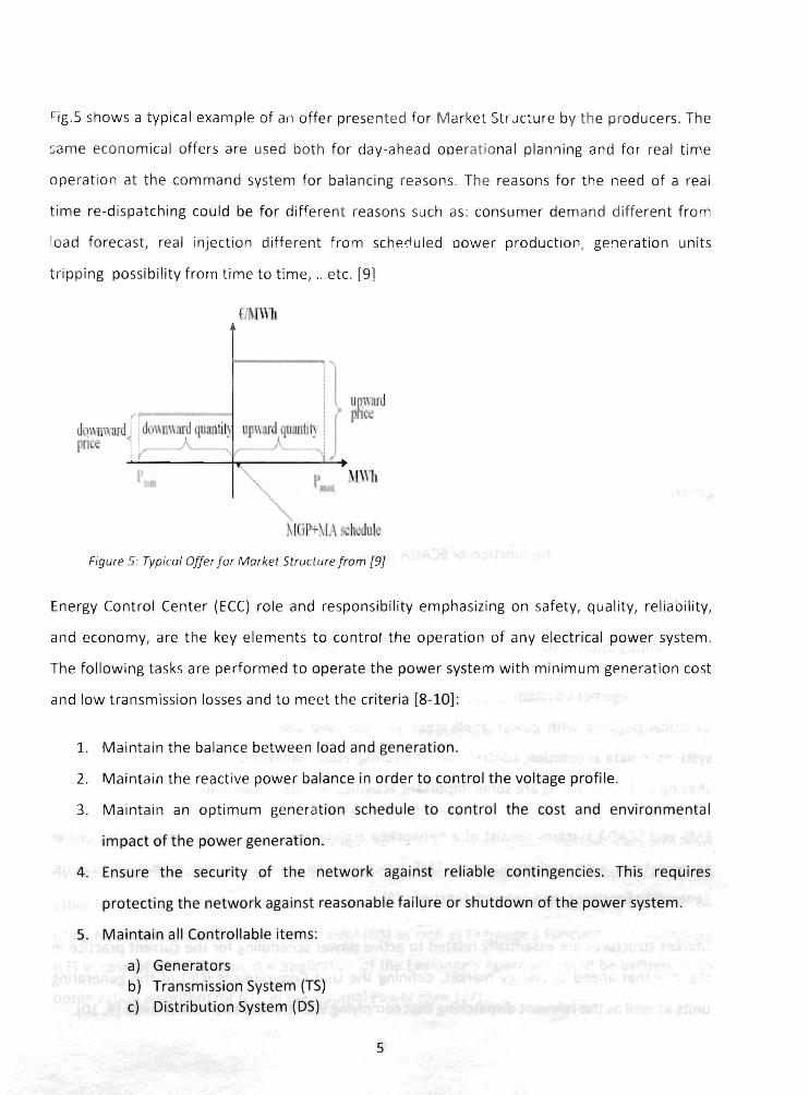
~ig . s shows a t ypical example of a,l offer presen ted for M arket Str'Jcture by the producers. The

same economica l offers are used both for day-ahead operatio nal p lanning and for real t ime

operation at t he command system for balancing reasons. The reasons for the need of a real

t ime re-dispatching could be for different reasons such as: consumer demand different from

load foreca st, real injection different from scheduled power production; ge'1eration units

tripp ing possibility f rom time to time, .. . etc. [9 ]

f~nYh

i l" l\mrd r : f plce

Jq\\lnYur( d \\Jl\\ard qU3l1t il~ up\\tml qU31\11 t~ : pnce ~~!

p M\\l. \

Figure 5 .' Typical Offer for Market Structure from [9J

Energy Control Center (ECC) role and responsibility emphasizing on safety, quality, reliability,

and economy, are the key elements to control the operation of any electrical power system.

The following tasks are performed to operate the power system with minimum generation cost

and low transmission losses and to meet the criteria [8-10]:

1. Maintain the balance between load and generation .

2. Maintain the reactive power balance in order to control the voltage profile.

3. Maintain an optimum generation schedule to control the cost and environmental

impact of the power generation.

4. Ensure the security of the network against reliable contingencies. This requires

protecting the network against reasonable failure or shutdown of the power system.

5. Maintain all Controllable items:

a) Generators b) Transmission System (TS) c) Distribution System (OS)

5

6. Person in-charge: "load Dispatcher" and "Independent System Operator (ISO)".

7. Schedules all the generating stations power output.

8. Controls other critical controls of the system like transformer taps setting, etc.

9. Monitors through a system called Supervisory Control and Data Acquisition (SCADA).

Takes corrective action as required.

10. Office is referred to as the Energy Control Center or Load Dispatch Center (LDC).

In case the loads and networks configuration changed, the state of the power network will not

change, which makes it more difficult to operate the power system. Also, the response of many

power network machines is not prompt. That's why changing trends and growth have increased

the need for computer-based operator support in interconnected power systems [8-10].

Two control centers are normally implemented in EEC are (EMS) for the operation of the

generation-transmission system, and (OMS) for the operation of the distribution system, which

is intended to help the dispatchers in monitoring and control of the system. The simplest of

such systems perform the function of SCADA (supervisory control and data acquisition system)

and others may have other sophisticated power application functions. The SCADA system

accepts telemetered data and displays them to operators has an alarm management subsystem

that monitors informs the operators of abnormal conditions [8-10].

Energy Management System (EMS) assists the operator (ISO) in monitoring and control of the

electrical network with power application software and contains all the features of SCADA

systems in data acquisition, control and monitoring. load management, loss minimization, peak

shaving and load shifting are some important activities of EMS implemented (8).

EMS and SCADA systems consist of a networked architecture of computers performing online

computations with backup support. EMS functions can be categorized as base functions,

generation functions, and network functions [8].

Market structures are essentially related to active power scheduling for the current practice in

the day that ahead of energy market, defining the Unit Commitment (UC) of the generating

units as well as the relevant dispatching that complying with transmission constraints [9, 10].

6

r

· - - ~ ~~ .. ~~ ... 't!t:*".. _.

y "t,\:~lt.,.r "',;;,> ~, -,( ,._, " ,~~ ffl>~ '" t ~ ~ ~.II _ ~~~.~ , ... ~ ..... y. • .L~~j;~(.1o.>"","",+""'''''''';';',,, Ii.~ "~~~.:.,_ •• ,,__ .• ~!. ':" 0'~." .~:.:£~~'\t~::(t.Z~;~~;l{~·~~l~;jj.;;'·

I ~

r

3. OPF Surveys

Comprehensive Surveys considered for a lot of papers in the field of optimal power flow

(OPF). In this project, different approaches to solve the OPF problem for any power system

were studied. Each technique and method will have its Pros and Cons.

Optimization methods and techniques, which have been used in solving the OPF problems,

have wide variety of techniques, such as Newton-Raphson (NR) based techniques [11, 12],

interior point methods [13, 14], quadratic programming [15, 16], non-linear (NlP) programming

[17-21], linear programming (lP) [22-24], sequential unconstrained minimization technique [25]

and other different practical techniques of optimization from different surveys [26-29].

Effective OPF is limited first by the high dimensionality of power systems, and second by the

incomplete domain dependent knowledge of power system engineers. The first limitation is

addressed by numerical optimization procedures based on successive linearization using the

first and the second derivatives of objective functions and their constraints as different

searches directions or by linear programming solutions to imprecise models. From the practical

methods of optimization was stated that the advantages of such methods are in their

mathematical foundation, but disadvantages exist also in the sensitivity to problem

formulation, algorithm selection and usually converge to local minima. The second limitation,

incomplete domain knowledge, prevents also the reliable use of expert systems where rule

completeness is not possible [4].

One of the Optimization methods is linear Programming (lP) and Non-linear Programming

(NlP). LP and NLP offer a powerful technique to most of power system optimization problems

by increasing the availability of high performance computers at relatively low costs [17-24]. On

other hand, lP and NLP optimization technique solve global optimization searching problems by

using Newton Raphson (NR) or Gauss-Seidel (GS) as well as lagrange's Function and multipliers

(LF) in case of NLP [4]. Also, the application of the Lagrange's Approach could be utilized as an

optimization algorithm for NLP in the Optimal Power Flow [27].

7

4. Wind Generation Technology in OPF

One of the most important challenges in the current and coming years is the optimization

control, like the optimal power flow (OPF) including wind generation technology and with

consideration of the wind generation cost [30-371.

Dynamic optimal power flow (DOPF) is "a typical complex, multi-constrained, non-convex, non­

linear programming problem in wind power integrated system" [371.

4.1. Green Energy Types:

There are different sources of Energy such as Fossil Fuels (Le. coal, Natural gas and diesel),

Nuclear Power, Hydro Electric Power and the green power [30]. Also, there are a lot of

comprehensive surveys in the Renewable Energy types as a green power generation. From the

Wikipedia references, we could summarize the types of Green Energy as below:

Green energy is created from natural resources that do not cause harmful pollution to Earth's

surface or atmosphere. With the concern of global warming and reducing the natural resources,

,. !

environmentally friendly alternatives are needed. Earth's sun, water and wind power have been r

used to operate machinery and generate power since ancient times. "The different types of

green energy that are currently being considered as alternative sources of power could be

described as below [301:

1. Hydropower converts water from rivers into usable energy released from turbines.

Today, it is considered very expensive and difficult to build hydropower plants to

produce mass amounts of electricity. There are also concerns that their usage may

affect wildlife and change the quality of the water [30].

2. Geothermal energy is produced from steam or hot water from under the Earth's

surface. The steam powers electric generators by rotating turbines. One use for it is

heating buildings. It is not widely available due to the lack of natural land sites. There

are also concerns that geothermic fields may eventually reduce. It is a green energy due

8

,

r

l

to its low emissions. Its production is not affected by weather changes and can

continuously work day and night. There are also some concerns about geothermal fields

affecting the surrounding land's stability [30].

3. Wind energy can be used to create energy by rotating large propellers like blades

around a hub. The blades slow down the speed of the wind it captures and channels it

to a generator that produces electricity. Wind energy usage worldwide is very small; the

technology is expensive and its machinery is considered to be noisy. The energy it

produces generates no pollution and has been used to power homes and farms [3~).

4. Solar energy is another form of green energy. Photovoltaic cells can absorb light from

the sun to capture electrons and use them to generate electricity. The sun has been

used as a source of energy since ancient times. However, it is still considered to be

expensive due the cost to produce the photovoltaic celled panels needed to generate

energy. These types' panels are usually large and take up a lot of space. Solar energy is

also inconsistent and needs a large surface area to generate enough electricity on a

large scale. Solar energy is being used to power some homes, cars and in agriculture.

5. Hydrogen is another source of energy that is eco-friendly. It's a common element that

can produce an unlimited amount of energy using water and electricity. Hydrogen was

once thought to be too dangerous to work with, but it is now being considered as a

source of fuel for vehicles. No emissions are created when used in its purest form. Only

water is released as a result. It is expensive to produce and store. More research and

time will be needed before it could be used on a worldwide scale" [30].

4.2. Cost Comparisons of Green Energy Supply Technologies:

It is well known that the conventional OPF problem only involved the thermal energy power

sources [31]. However, with the introduction and development of the renewable energy

sources specifically the wind energy [32] started the necessity to incorporate the wind

generation cost into the classical OPF problem. Several of literature [31- 37] have been

published in investigating the OPF problem with wind generation cost involved.

9

'-

The Electricity Generation costs estimates based on a single station developed with a prototype

built and tested, as shown in Table 1, based on the reference from the website of the cost

comparisons of energy supply technologies [38]. From this website, we have a got a chance to

compare the electricity generation costs for numerous green energy supply technologies.

Table 1: Cost Comparisons of Energy Supply Technologies, dated April 28th, 2011 from [38]

Energy Supply Coal Fired

Geothermal Wind Farms

Technology Type Nuclear Solar Tower Steam

Estimated life Cycle 25 years 25 years 60 years 15 years 25 years

(in years)

Gross output 1000 MWjhr. 1000MWjhr. 200 MWjhr. 300MWjhr. 200MWjhr.

Net output (MWjhr.) 900 815 195 270 190

Output efficiency 90.00% 81.50% 97.50% 90.00% 95.00%

CAPITAL COSTS

Design Cost $100M $750M $150M $250M $100M

Test Plant Not required $1,OOOM $150M $500M Not required

Materials/Equipment $700M $1,000M $400M $550M $800M

Cost

Construction Cost $250M $500M $250M $350M $300M

Labour Cost $250M $500M $90M $200M $150M I

Total Capital Costs $1,300M $3,750M $1,040M $1,850M $1,350M

OPERATIONAL COSTS

Interest @ 6% $78M $225M $62.4M $111M $81M

Fuel Cost $200M $400M $0 $0 $0

FuellWaste Disposal $100M $250M $0 $30M $0

Cost Water use (including

$100M $300M $250M $15M $0 mining process)

Maintenance Costs $150M $375M $10M $50M $100M

OPERATIONAL $628M $1,550M $322.4M $206M $181M

COSTS

TOTAL COSTS

Net Yearly Cost (Life/Capital) + Yearly $1,271.3M $1,502.8M $1.a7S.2M $89.983M $131.417M Running Cost

Production Cost $0.16 $0.26 $0.05 $0.15 $0.14

$/KWH

10

I r , [ I • (

r ( (

[

r r r

i r

i (

r

r r

r

As shown in Table 1, the electricity generation costs for different type of energy is estimated

based on a single station developed with a prototype built and tested. The Total Capital Costs

for the Nuclear power plant is the most expensive one comparing with other types of energy, as

shown in Fig.G.

Total Capital Costs (Million Dollar $) $4,000 .,....--------~"-----­

$3,500 +---­$3,000 +----­$2,500 +----­$2,000 +---­

$1,500 +---­

$1,000

$500

$0

III Total Capital Costs (Million Dollar $)

Figure 6: Total Capital Costs (M$) for different types of energy

As show in Fig.7, also the Operational Costs for the wind generation is the minimum. However,

the Nuclear power is the most expensive one comparing with other types of energy.

OPERATIONAL COSTS (Million Dollar $) $2,000.0 $1,500.0 +1 ___ _

$1,000.0

$500.0

$0.0

Figure 7: Operational Costs (M$) for different types of energy

11

III OPERATIONAL COSTS (Million Dollar $ )

Generally, the Nuclear power energy has the most expensive total capital cost to establish a

nuclear power plant as well as the most expensive operational costs comparing with other

power generation plants. However, the net yearly cost (life/capital) including the yearly running

cost could be considered as economic power generation unit comparing with some other

conventional energy. On other hand, it was very clear that the green energy especially the wind

generation is considered as economical cost generation, as shown in Fig.8.

Net Yearly Cost (Ufe/Capital) + Yearly Running Cost (Million Dollar $)

$2,000.00 -r-------------­$1,500.00 +---­$1,000.00

$500.00

$0.00

.. Net Yearly Cost (Ufe/Capital) + Yearly Running Cost (Million Dollar $)

Figure 8: Net Yearly Cost (Life/Capital) including Yearly Running Cost (M$) for different types of energy

Generally, one of the most important challenges in the current and coming years is the OPF

including wind generation technology and the consideration of the wind generation cost in the

OPF for the entire power system as in our case study. The wind generation cost based on the

reference from the website of the cost comparisons of energy supply technologies, dated on

April 28th, 2011 [38], is estimated as 0.14$/KWH for the production cost, as shown in Fig.9.

Production Cost $/KWH $0.30 .,..----------------­$0.25 +----­$0.20 +------, $0.15 $0.10 $0.05 $0.00

.. Production Cost $/KWH

Figure 9: Power Production Cost ($/KWH) for different types of energy and power generation plants

12

r I I { I'

i

r.

r r

...

I \

r

( (

I /

{ ! r

r>

r

5. THEORY OF OPTIMAL POWER FLOW (OPF )

During the comprehensive surveys that considered a lot of papers in the field of optimal

power flow (OPF). I have found that one of the best researchers that explained the OPF theory

in a very organized way is Tarek BOUKTIR and Linda SUMANI [41, in addition to what learned

during the course of Power System Optimization Course [7] and other survey papers in the field

of OPF [11-29}.

In this project, and from thoroughly study for different surveys, different approaches to solve

the OPF problem for any power system were studied.

5.1. OPF Problem:

The Optimal Power Flow (OPF) has been usually considered as the minimization of an objective

function representing the generation cost and/or the transmission losses. The constraints

involved are the physical laws that leading the power generation and transmission systems, as

well as the operating limitations of the entire power system and equipment [4-29].

5.2. OPF Solutions & Results:

Effective Optimal Power Flow is limited by the high dimensionality of power systems and the

incomplete domain dependent knowledge of power system engineers. [4-29]

A practical method is given for solving the Power Flow problem with control variables such as

real and reactive power and transformer ratios automatically adjusted to minimize

instantaneous costs or losses. The solution is feasible with respect to constraints on control

variables and dependent variables such as load voltages, reactive sources, and tie line power

angles. The method is based on power flow solution by Newton's (NR) method which modified

to Fast Decoupled Power Flow (FDPF) as in the commercial use.

13

------ .. --.. --... ~-~~ ... ---

Due to its quadratic convergence, the NR method that have modified to Fast Decoupled Power

Flow, has rapid convergence independent from system size. However, as the system size

(number of equations) increases, the function evaluation at each iteration will be increased.

Comparison between three different scenarios for our case study is done by using Fast

Decoupled Power Flow (FDPF) with a result that shows the performance of FDPF. All results and

data will be discussed later on in this project. Also, full study is done on our case study for three

different scenarios for power load flow computation. The code can implement the Algorithm of

the power load flow using the FDPF and find the maximum mismatch in the control variables of

the real and reactive power for any number of buses that let the algorithm to converge.

The challenge in algorithm development is to effiCiently identify the binding inequalities. This

logarithmic corresponding to the original problem (OPF) is solved by the FDPF method.

The advantages of such methods are in their mathematical foundation, but disadvantages exist

also in the sensitivity to problem formulation, algorithm selection and usually converge to local

minima. The second limitation, incomplete domain knowledge, prevents also the reliable use of

expert systems where rule completeness is not possible.

During the comprehensive survey in the OPF field and in the development and adaptive

algorithms, some of the Optimization methods considered as a good optimization tools for the

OPF such as Linear Programming (LP) and Non-Linear Programming (NLP). LP and NlP offer a

powerful approach to these Optimization Problems made possible by the increasing availability

of high performance computers at relatively low costs. Also, LP and NLP optimization technique

solve global optimization searching problems by using Newton Raphson or Gauss-Seidel as well

as lagrange's Function and multipliers in case of NlP. The controllable variables are

decomposed to active constraints that effect directly the cost function are included in the NlP

and passive constraints which are updating using a conventional load flow program, only, one

time after the convergence. The slack bus parameter would be recalculated in the load flow

process to take the effect of the passive constraints [4].

14

1 ( r ,

{; I J

r­

r

f

r

1 ( I

I

I r

\,

I r r r

r ,

5.3. Problem Formulation:

The standard OPF problem can be written in the following form [1-381,

Minimize: F(x)

Subject _ to : x tnin < x :::; x max

gj (x) = bjVi = 1,2 ... ME

h j (x) :::; c j Vi = 1,2 ... MI

(1)

where F(x) is the objective function, g(x) represents the equality constraints, h(x) represents the

inequality constraints and is x is the vector of the control variables, that is those which can be

varied by a Control Center Operator (e.g. generated active and reactive powers, generation bus

voltage magnitudes, transformers taps etc.).

The essence of the OPF problem resides in reducing the objective function and simultaneously

satisfying the Load Flow Equations (equality constraints) without violating the (inequality

constraints), which are the Physical System Limits at all generator buses and Operating System

Limits at load buses [4].

5.4. Objective Function:

The most commonly used objective in the OPF problem formulation is the minimization of the

total cost of real power generation. The individual costs of each generating unit are assumed to

be function, only, of active power generation and are represented by quadratic curves of

second order [4, 7]. The objective function for the entire power system can then be written as

the sum of the quadratic cost model at each generator:

NG NG

F(x) = CPTotal = IC~ = I(a j +bj.Pgj +c j .Pg j

2) (2)

j=! j=l

Where:

NG is number of generation including the slack bus.

Pgi is the generated active power at bus-i.

ai, bi and ci are the unit costs curve for ith generator.

15

~ ____________________________________________________ .J

5.5. Types of Equality Constraints:

While minimizing the cost function, it is necessary to make sure that the generation still

supplies the "load demands (Pd) plus losses in transmission linesll• Usually the Power Flow

equations are used as equality constraints:

(3)

Where Active and Reactive Power injection at (bus i) are defined in the following equation:

N

F;(V,B) = V; *::L[VjY;j *COS(Oi -OJ -Bij)] j=1

N

Qi(V,B) = V; *::L[VjY;j *sin(oi -OJ -Bij)] j=l

NB

'p;(V,O) == 2:Vi,Vj'(gif cosOif +bif sinBif ),i = 2,NB j=1

NB

Qj(V,B) = 2:V;,Vj'(gif sin0if -bif cos Bif),i = NPV + I,NB j=i

Where:

Yij is the Bus Admittance

gij is the Conductance, and bij is the Susceptance

Vi is voltage magnitude at the bus i and e ij is the bus voltage phase angle.

(4a)

(4b)

The real power balance and reactive power balance are the most important in OPF and they

considered as Equality Constraints [7].

5.6. Types of Inequality Constraints:

The inequality constraints of the OPF reflect the limits on physical devices in the power system

and the operating limits created to ensure system security. The most usual types of inequality

16

I

i t

\ , ,

~:­>-

constraints are upper bus voltage limits at generations and load buses, lower bus voltage limits

at load buses, var. limits at generation buses, maximum active power limits corresponding to

lower limits at some generators, maximum line loading limits and limits on tap setting and

phase shifter. The inequality constraints on the problem variables considered include [4, 7]:

• Upper and lower bounds on the active generations (Real Power) at generator buses:

Pgi min::; Pgi ::; Pgi max, where (i = 1, NG) (5)

• Upper and lower bounds on the (Reactive Power) generations at generator buses and reactive

power injection at buses with VAR compensation:

Qgi min::; Qgi::; Qgi max, where (i = 1, NPV) (6)

• Upper and lower bounds on the voltage magnitude at the all buses:

Vi min::; Vi ::; Vi max, where (i = 1, NB) (7)

• Upper and lower bounds on the bus voltage phase angles:

8i min::; 8i ::; 8i max, where (i = 1, NB) (8)

- • Upper and lower bounds on branch MW/MVAR/MVA flows may come from thermal ratings of

conductors, or they may be set to a level due to system stability concerns:

(9)

Finally, the generalized objective function F is a non-linear, and the number of the equality and

inequality constraints increase with the physical size of the power distribution systems.

Different applications of a conventional optimization technique such as the gradient-based

algorithms to a large power distribution system with a very non-linear objective functions and

great number of constraints are not good enough to solve this OPF problem. Because it depend

on the existence of the first and the second derivatives of the objective function and on the

well computing of these derivative in large search space [4].

17 PP.CcPf.f'.rt Of.· ,

R'lmsc-~ ~~)W!fmY·trnRARV

6. Project Case Study Using OPF Methodology

6.1. Discussion and Theory:

In this project the most optimal solution of optimal power flow (OPF) incorporating wind

generation cost was studied, to supply power to a new residential compound load located at

the outskirts of an industrial area for three different scenarios. This domestic load is typical of

long rural line with isolated load area.

An interconnected network is generally found in more industrial or urban areas and would have

almost multiple connections to other power supply. The benefit of interconnected model is that

in case of a fault and/or maintenance a small area of network would be isolated and the rest

kept on supply. This represent the scenario one of our case study to feed both the industrial

area as well as the long rural line domestic load in the village. However, the challenging in our

case study that we have to incorporate a wind generation unit as one type of green energy, that

are currently being considered as an alternative source of power, to feed this long rural line for

the domestic load without effecting in the total generation cost.

A case study conducted for three different scenarios incorporating wind generation cost to feed

this long rural line for the domestic load. The results of OPF shows that incorporating wind

generation cost as renewable energy source with the entire power system will have a minimum

generation cost and minimum transmission losses even if the wind generation cost assumed to

be the most expensive one comparing with other conventional generation units.

In this project, it's succeeded to have the required code to implement the Algorithm of the

Power Flow using the FOPF and find the maximum mismatch of the real and reactive power for

any number of buses and let the algorithm to converge. This program succeeded to optimize

the best solution for three different scenarios by using (fmincon) as one of optimization tools to

achieve the minimum total cost function of generating units and minimum transmission losses.

18

r r

i ~

r

r I I

I

r

ISO would like to minimize the total cost incurred to purchase real power as required to serve

the load(s) and supply for losses in the transmission system. This solution must satisfy physical

and operational criteria as set by physical characteristics and the law of the land.

The variables at hand and segregate them as those that we may wish to control (control

variables) and those that assume values as a result of settings of the control variables and the

physical system (dependent variables).

List of variables:

PG - Real power output of generators

QG - Reactive power output of generators

VG - Magnitude of Voltages set at the terminals of generators

Vl- Magnitude of Voltages set at load buses

{) - Phase angles of all Bus voltages phasors

List of constraints characterizing the physical system and loads:

• (r, x, zl, yl and V) - Transmission line resistance, inductive reactance, complex

r impedance, and complex admittance and shunt line charging capacitive admittance.

• (VB): System Admittance matrix in the bus frame of reference (complex).

• (PO, QO) - Real and Reactive power drawn at buses by connected loads.

Now, from the above, we could identify the objective and constraints:

Objective Function:

The cost of real power from the ith generator is specified as:

CPi = l:(ai + bi . PGi + ci . PGi2} ; (10)

The total cost incurred by the system operator at the energy control centre would be equal to:

CP = l: CPi = l:i (ai + bi . PGi + ci . PGi2) (11)

19

So, the objective of the problem would then be:

Minimize: CP = L CPi = Li (ai + bi . PGi + ci . PGi2) (12)

Constraints \

Power Balance Transmission System Constraints at every Bus:

PGi - POi - Pi (V, 0) = 0 Real Power Balance (13)

QGi - QDi - Qi (V, 0) = 0 Reactive Power Balance (14)

>' . Physical Device Limits at Generators:

PGi min < PGi < PGi max (is) 1

QGi min < QGi < QGi max (16) .. f I

VGi min < VGi < VGi max (17) I J

System Operating Limits at load Buses: r > 1

VLi min < VLi < VLi max (18)

010 = 00 (19) r

r 6.2. PROJECT PROPOSAL (CASE STUDY):

Selecting the most optimal way (OPF) to supply power to a new residential compound load (

located at the outskirts of an industrial area. The area is settled for three big

industrial facilities with a bulky load supplied by two generation stations, one from the north

(low generation cost) and the other one in the south (high generation cost) of the industrial

area. Now, the industrial area authority decided to build a new village far from the industrial

area to the south west direction. Also, a transmission line will be built to connect the industrial

area and residential village (compound) with a fixed capital cost.

20

1 ~

t J l > 1

r r I

r i

This project is studying three (3) different scenarios:

1. PROPOSAL-l: Feeding the Residential load (Village) from two generating units, as shown

in Fig.10. The project studying how to optimize the load sharing between the two

generators with consideration that the nearest one to the Village has (high Generation

Cost but with less power losses) and the other far one has (low Generation Cost but with

more power losses) in the transmission system.

P=25MW Q=5MVAA

Bus3

Gl~ Bus 1

P=30MW . .....---., Q = 10 MVAA

Bus 6

.............. --". P = 50 MW Q=S MVAR

Figure 10: OPF Case Study (Scenario-l) for feeding a new residential/oad from the same generating units

of the Industrial Area

21

2. PROPOSAl-2: Installing a Wind Generator (as a good example for the Green Energy)

beside the Village to feed the Residential load, while keeping the transmission line

totally disconnected from the Industrial Area, as shown in Fig.ll. Then, start to optimize

the Objective Function which is the Total Generation Cost.

Bus 8

~ P=5SMW

0.=13

P=55MW f-0.:13 \r-

....... Bus2

P=30MW

0.=18

P=50MW o.:5MVAR

Figure 11: OPF Case Study (Scenario-2) for feeding a new residential load from a Wind Generation Unit

with disconnected T.L with other generating units of the Industrial Area

22

,1 1 f ,

l r I" ) ,

"

~

1 1

!

,1 1 f 1

l r l'· r

b

3. PROPOSAl-3: Optimize the Power Flow with consideration that the two Generation

Stations beside the Industrial Area and the Wind Generator beside the Village will be

connected with same Power System Network, and the Project studies how to optimize

the load sharing between all the Industrial and Residential loads, as shown in Fig.12.

BusS

~I"l IT Bus 7

P=25MW

Q=SMVAA

P=55MW

Q=5MVAR

Gl~ Bus!

Bus3

--.... Sw2

P=30MW

0=10

Figure 12: OPF Case Study (Scenaria-3) for feeding a new residential load from the entire power system

with consideration of the Wind Generation Cost

23

6.3. Project Result Analysis:

A case study conducted for all the three different scenarios incorporating wind generation cost,

as shown in Table 2.

Table 2: Test Results Analysis for Three Different Scenarios (all results attached in the Appendix)

RESULTS PROPOSAL-1 PROPOSAL-2 PROPOSAL-3

TOTAL REAL GENERATION (MW) 176.926560 172.824448 172.523911

TOTAL REAL GENERATION (MW) 160.000000 160.000000 160.000000

TOTAL TRANSMISSION lOSS (MW) 16.926560 12.824448 12.523911

TOTAL COST ($) 64,768.2154 73,689.4818 50,892.0832

The results of OPF show that incorporating wind generation unit as renewable energy source

with the entire power system will outcome to have a minimum generation cost and minimum

transmission losses for the entire power system, as shown in Fig. 13 and Fig. 14.

80000

70000

-60000 -en. ;:: 50000

VI 8 40000

tii 30000 .... {2 20000

10000

Total Generation Cost in $

o ~-------------.-------------~~-------------,( 1 2 3 Proposals

Figure 13: Comparison oj Total Generation Cost ($) based on OPF results

24

r t ,i

r ,

r \

r

",

'" ~

1

i r r .,

i

t \ ~

Transmission losses in MW

-~ 20 ~ -III 15 OJ III III 10 0 ..... c:

5 0 III III .- 0 E III

1 2 3 c: fa

~

Figure 14: Comparison of Transmission Losses (MW) based on OPF results

Optimal Power Flow (OPF) problem was solved in this project by using MATlAB optimization

method and technique on computer. The toolbox (fmincon) has become standard practice to

solve a lot of optimization problems. This toolbox from MATlAB has three algorithms, with

. several options for Hessians, including fmincon trust region reflective algorithm, fmincon active

set algorithm, and fmincon interior point algorithm.

The Project used fmincon Optimization Toolbox from the MATLAB to optimize the objective

function which is the total generation cost. It was clear that the power transmission losses will

account for more Power generation cost. The constraints and the bounds of the optimization

problem were the normal physical limits for operating any power system. All the test results of

the three different scenarios are attached in the Appendix for the minimum generation cost

and transmission losses for the entire power system.

25

7. Conclusion and Future Work

The OPF problem is the Optimal Power Flow for a power system operation with an objective

function, Total Generation Cost, is optimized while satisfying set of system operating

constraints.

OPF has been widely used in power system operation and load flow planning. The OPF is a

nonlinear, non-convex, large-scale, static optimization problem with both continuous and

discrete control variables. Mathematical programming approaches, such as linear, and

nonlinear programming, and interior point methods have been used for the solution of the OPF

problem.

The challenging was in our case study to incorporate a wind generation unit as one type of

green energy, to feed this long rural line for the domestic load without effecting in the total

generation cost. A case study conducted as per the achieved results mentioned above, for a"

the three different scenarios incorporating wind generation cost. The results of OPF shows that

incorporating wind generation unit as renewable energy source with the entire power system

will have a minimum generation cost and minimum transmission losses for the entire power

system even if the wind generation cost assumed to be the most expensive one comparing with

other conventional generation units.

One of the most important challenges in the current and coming years is the optimal power

flow (OPF) with consideration of the wind generation cost. The wind generation is considered

as dynamic optimal power flow (DOPF) which is a typical complex, multi-constrained, non­

convex, non-linear programming problem.

Green Energy is created from natural resources that do not cause harmful pollution to Earth's

surface or atmosphere. With the concern of global warming and reducing the natural resources,

environmentally friendly alternatives are needed. The different types of green energy that are

currently being considered as alternative sources of power could be studied in the future work

26

I , I

r r

( f

t

r

.. \

" \

'\

r r

\

t

with consideration of the generation cost and its effect on the OPF of the entire power system.

That's why; there are a lot of challenges of adhering standards, technology and cost challenges.

Using Genetic Algorithms (GA) as another MATLAB optimization toolbox in the future works for

the same case study with all different scenarios may be could achieve better results than

fmincon toolbox. The application of genetic algorithms (GA) in solving the OPF problem,

overcomes the limitations of the conventional approaches in the modeling of non-convex cost

functions, discrete control variables (such as switchable shunt devices, transformer tap

positions, and phase shifters, further complicates the problem solution.), and prohibited unit

operating zones. GA has been developed as a biological approach to search and optimization.

They consist of a population of bit strings transformed by three genetic operators: selection,

crossover and mutation. Each string (chromosome) represents a possible solution for the

problem being optimized and each bit (or group of bits) represents a value for some variable of

the problem (gene). These solutions are classified by an evaluation function, giving better

values, or fitness, to better solutions .

. There are a lot of well-known features of GA as an optimization tool for solving OPF problems:

1. GA does not require "well behaved" objective functions and allow simple handling of

discontinuities and non-linearity, which are hard to include in pure mathematical

programming methods.

2. Using GA will not obtain only one "Optimal solution, but a large group of solutions

3. GA is well adapted for distributed implementations, allowing computation time to be

drastically reduced. The test results in the existing GA-OPF models are limited to small

problems, and usually simple fast decoupled load flow (FOLF) is used with no PV-PQ bus­

type switching, since generator reactive capabilities are incorporated in the functional

operating constraints.

27

References

[1] Hermann W. Dommel, and William F. Tinney, "Optimal Power Flow Solutions", IEEE

transactions an Power Apparatus and Systems, PAS-87, No.l0, October 1968.

[2] M. A. Abido, "Optimal power flow using particle swarm optimization", Electrical Power and

Energy Systems 24 (2002) 563-571, ElSEVIER Science ltd., 2002.

[3] Edmea C. Baptista, Edmarcio A. Belati, Geraldo R.M. da Costa, "logarithmic barrier­

augmented lagrangian function to the optimal power flow problem", Electrical Power ond

Energy Systems, Elsevier ltd., 2005.

[4] Tarek BOUKTIR, and linda SlIMAN!, "Optimal Power Flow of the Algerian Electrical Network

using an Ant Colony Optimization Method", Leonardo Journal of Sciences, ISSN 1583-0233,

2005.

[5] William H. Kersting, IiDistribution System Modeling and Analysis", CRC Press, 2002.

[6) William Stevenson and John Grainger, "Power System Analysis", McGraw-Hili Science

Engineering, 2005.

[7] Venkatesh B, "Power System Optimization" in ECE website, EE8604, RU, 2009.

(8] Energy Control Center Website: http://www.scribd.com/doc!20328427!Ee1401-Power­

System-Operation-and-Control-Energy-Control-Center-Safety; Accessed on April 28th, 2011.

[9] F. Bassi, C. Bruno, P. Crisafulli, G. Giannuzzi, l. Gorello, S. Pasquini, M. Pozzi, and R. Zaottini,

"Optimal Power Flow procedure for real-time security and economic re-dispatching in a market

structure", IEEE, 2009.

[101 lee K. V., Park V. M., and Ortiz J. l., "A United Approach to Optimal Real and Reactive

Power Dispatch", IEEE Transactions on Power Systems, Vol. PAS-104, p. 1147-1153, 1985.

[11] Sun 01, Ashley B, Brewer B, Hughes A, Tinney WF, "Optimal power flow by Newton

28

r r

f

,.. ,

J •

... ,

1 ,

-, .

':' •

r f

approach", IEEE Trans Power Apparatus System; PAS·I03(10):2864·75, 1984 .

[12] Santos A, da Costa GR, "Optimal power flow solution by Newton's method applied to an

augmented Lagrangian function", lEE Prac Gener Transm Distrib; 142{1}:33·36, 1995.

[13J Yan X, Quintana VH, "Improving an interior point based on OPF by dynamic adjustments of

step sizes and tolerances", IEEE Trans Power System; 14(2):709·17, 1999.

[14] Momoh JA, Zhu JZ, "Improved interior point method for OPF problems", IEEE Trans Power

System; 14{3):1114-20, 1999.

[15] Burchett RC, Happ HH, Vierath DR, "Quadratically convergent optimal power flow", IEEE

Trans Power Apparatus System; PAS·103:3267·76, 1984.

[16] Aoki K, Nishikori A, Yokoyama RT, "constrained load flow using recursive quadratic

programming", IEEE Trans Power Apparatus System; 2{1}:8·16, 1987.

[17] Sasson M., "Nonlinear Programming Solutions for load flow, minimum loss, and economic

- dispatching problems", IEEE Trans. on Power Apparatus and Systems, vol. Pas·88, No.4, 1969.

[18] Alsac 0, Stott B, "Optimal Load Flow with steady state security", IEEE Trans Power

Apparatus System; PAS·93:745·51, 1974.

[19] Shoults R, Sun 0, "Optimal power flow with based on P-Q decomposition", IEEE Trans

Power Apparatus System; PAS·I01(2):397·405, 1982.

[20] Happ HH, "Optimal power dispatch: a comprehensive survey", IEEE Trans Power Apparatus

System; PAS·96:841·54, 1977.

[21J Mamandur KRC, "Optimal control of reactive power flow for improvements in voltage

profiles and for real power los minimization", IEEE Trans Power Apparatus System; PAS·

\ 100(7):3185·93, 1981.

I r [22] Abou EI-Ela AA, Abido MA, "Optimal operation strategy for reactive power control,

29

Modeling, simulation and control", part A, vol. 41(3), AMSE Press, 1992.

[231 Stadlin W, Fletcher D, "Voltage versus reactive current model for dispatch and control",

IEEE Trans Power Apparatus System; PAS-101(10):3751-8, 1982.

[24] Mota-Palomino R, Quintana VHf "Sparse reactive power scheduling by a penalty-function

linear programming technique", IEEE Trans Power Apparatus System; 1(3):31-39, 1986.

[25] Rahli M, Pirotte P, "Optimal load power flow using sequential unconstrained minimization

technique (SUMT) method under power transmission losses minimization", Electrical Power

System Res;52:61-64, 1999.

[26] Fletcher R, "Practical Methods of Optimization", John Willey and Sons, 1986.

[27] Edmea C. Baptista, Edmarcio A. Belati, Geraldo R.M. da Costa, "Logarithmic barrier­

augmented Lagrangian function to the optimal power flow problem", Electrical Power and

Energy Systems, 27 (2005) 528-532, 2005.

[28] B. Venkatesh, G. Sadasivam, and M. Abdullah Khan, "A New Optimal Power Scheduling

Method for Loss Minimization and Voltage Stability Margin Maximization Using Successive

Multi-Objective LP Technique", IEEE transactians on Power Systems, VOL 15, No.2, May 2000.

[29] Bouktir T., Belkacemi M., Zehar K., "Optimal power flow using modified gradient method",

Proceedings ICEL'2000, U.S.T. Oran, Algeria, p. 436-442, 2000.

[30] Types of Green Energy Website: http:Uwww.ehow.com!about 4702917 types-green­

energy.html#ixzzlNgefs4aN; Accessed on April 16th, 2011.

[31] LB. Shi, C. Wang, L Z. Vao, LM. Wang, V. X. Ni, and B. Masoud, If Optimal Power Flow with

Consideration of Wind Generation Cost", International Conference on Power System

Technology, IEEE 2010.

[32] T. Ackermann, If Wind Power in Power System", Chi Chester: Wiley, 2005.

30

" -,

-j

.... , "

J

''";

) .

. ,

[33] Y. liu, T. Shang, ilEconomic Dispatch of power system incorporating wind power plant", in

Proc. 1991 power Engineering Conference, pp. 159-162, 1991.

[34] 1. B. Cardell, and C. l. Anderson, "Estimating the System Costs of Wind Power Forecast

Uncertainty", IEEE transactions, IEEE 2009.

[35J Haiyan Chen, Jinfu Chen, and Xianzhong Duan, "Multi-Stage Dynamic Optimal Power Flow

in Wind Power Integrated System", IEEE transactions, IEEEjPES Transmission and Distribution

Conference & Exhibition, 2005.

[36] R.A. Jabr, B.C.Pal, "Intermittent wind generation in optimal power flow dispatching", IEEE

transactions, The Institution of Engineering and Technology, 2008.

[37] Gonggui Chen, Jinfu Chen, and Xianzhong Duan, "Power Flow and Dynamic Optimal Power

Flow Including Wind Farms", IEEE Xplore, 2010.

[38] Cost Comparisons of Energy supply technologies Website:

www.unenergy.org!Popup%20pages!Comparecosts.html. Accessed on April 20th, 2011.

31

'Iii Err mtwWftjWPN -irimii ij fg aT"

Appendix:

1 PROJECT CODE:

The MATlAS code used (fmincon) Optimization Toolbox which used in the OPF project and

structured as below:

1. The program of the project named "Proj.m". This works on files "prop1.i" and "prop3.i".

These are the proposals 1 and 3, as show in Fig.(10) and Fig.(12).

2. The program "Proj2.m" works on "prop2.i". This is proposal 2. The program will work on

proposal 2 (Which has an open Transmission line) without any outside calculations. The

"Proj2.m" designed to work on it. Also, it can work on the other two proposals as well.

3. In the output files, you could find at the end the Total Transmission Losses and the Total

Generation Cost.

4. Compare between the proposals using these values. The results was showing that the

generation cost of proposal 3 (Scenario-3) is the lowest cost (S/MW) and lowest

transmission losses.

1.1 How Program Work (Brief Write-up):

The Programs (Proj.m) and (Proj2.m) will read input data from the input data files of the

proposals of the different systems, then build the (Admittance Matrix) and the (S' and S"

Matrices) for these systems.

Proj1.m will work for the proposals (1 and 3) by running the Load Flow algorithm using the Fast

Decoupled load Flow (FDLF) Algorithm. This will generate initial conditions for the Optimization

process to start with.

Proj2.m will work for proposal 2 and it will not run the load Flow Algorithm as the system will

then contain two isolated islands and values of unity will be assigned to load Voltage

32

"­)

i

.;

-: ... .. ;

,.

i r

-'j , ,

" ~-;

i

T r r I

I

I

r

r

Ii iii ril nflflSlalllEI

Magnitudes and values of zero will be assigned to Voltage Angles, Real Power and Reactive

Power initially. Consequently it will not contain parts 6 and 7.

Then both programs will execute part_8 by running the Optimization using the (fmincon)

function which applies non-linear constrained optimization. In this part upper and lower

bounds for the Variables.

An external function called (Constraints.m) will be used to apply the non-linear constraints for

the Power Balance Equations. After that the Transmission line Flows will be done and the

Output files will be created containing all the calculations for the system including the

Transmission losses and the Total Generation Cost.

1.2 Project Code Description:

Part_l: Read Data File and Input System Data & Details

1. % Transformer Part 2. % Transmission line Part

3. % Shunt Capacitors Part

4. % Shunt Reactors Part

Part_3: Y bus partitioning (Y&Th)

Part_ 4: Formation of B prime (BP) Matrix

Part 5: Formation of B double prime (BDP) Matrix

Part_6: Starting FDlF Algorithm

FDlF Algorithm Conditions:( IT<=ITmax && ERR>=TOLER/Pbase) to enter Algorithm loop

1. Stepl: Calculate (P) at all buses

2. Step2: Calculate (DeIP) = {PG-PD-P} at all buses except Slack Bus

3. Step3: Calculate (DeIDel)at all buses except Slack Bus

33

; " f ,_._;<~_.I., ".f;'" ,I .. -_K,.J;IJ,P __ =.,·.· ';=f"'~:";f_ F~ ~i·'Z!Z < • •• ,." tM!-··~T'·;·'·!,;k:" · ·"'f ,·.'.· .. "·f·;··.., tTI·'fwf~a' t tt ,-t'iF'W -t: rr t; ::::;;i=g j§ii uwa;; 1m .

4. Step4: Update the value of Delta (DEl)

5. StepS: Calculate (Q)at all buses

6. Step6: Calculate (DeIQ)=(QG-QD-Q) at all buses except Gen. Buses

7. Step7: Calculate (DeIV) at all buses except Generator Buses

8. Step8: Update the value of (V)

9. Step9: Check the Convergence: ERR = max(PMIS,QMIS)

*Note: (1): Add one to the number of iterations (IT=IT+l) (2): Check for Convergence: If still (ERR>TOLER/Pbase) & (IT<3), then GO BACK to Step1

again, till it will be converge or be finished the 3-iterations and stop.

Part_7: Calculate Real and Reactive Power Generated

Part_8: Run Optimization

• Set Lower and Upper Bounds

• Initial Conditions

• linear Constraints

*Note: The non-linear constraints are calculated by the function Constraints.m

• Defining Objective

• Invoking the 'fmincon' routine

• Updating variables

Part_9: Calculate Transmission line Power Flow

y 1st: Real and Reactive (From Flow) and (To Flow) Part

y 2nd: Power Flow (MVA) per Circuit Part

Part_lO: Generate Output file to write the output data, summary of the results, Transmission

Losses and Total Cost

34

f ~

1

"

J r r

~ 1 \

,. "

,,' .

J T

2 PROJECT RESULT ANALYSIS:

Proposal-l Results:

INPUT FILE NAME: propl.i OUTPUT FILE NAME: prop1.o SYSTEM: IEEE 6 BUS SYSTEM YEAR 2011 CASE PEAK LOAD NUMBER: 100 NUMBER OF BUSES : 7 SLACK BUS NUMBER : 1001 NUMBER OF GENERATORS : 2 NUMBER OF LOAD BUSES : 5 NUMBER OF TRANSFORMERS 2 NUMBER OF TRANSMISSION LINES NUMBER OF SHUNT CAPACITORS :

: 1

NUMBER OF SWITCHABLE CAPACITORS NUMBER OF SHUNT REACTORS : 1 SLACK BUS VOLATGE : 1. 0500 TOLERANCE (MW) 0.0100 BASE MVA 60 : 100.0000

6

: 1

MINIMUM LOAD BUS VOLTAGE : MAXIMUM LOAD BUS VOLTAGE :

0.9000 1.1000

MAXIMUM NUMBER OF ITERATIONS : 3

ITERATION :1 MAX P MISMATCH ITERATION : 1 MAX Q MISMATCH

. ITERATION :2 MAX P MISMATCH ITERATION :2 MAX Q MISMATCH ITERATION :3 MAX P MISMATCH ITERATION :3 MAX Q MISMATCH

SUMMARY OF THE RESULTS ----------------------

TOTAL REAL GENERATION TOTAL REAL LOAD TOTAL REAL LOSS

TOTAL REACTIVE GENERATION TOTAL REACTIVE LOAD TOTAL REACTIVE LOSS

TRANSMISSION LOSS

= = =

=

=

=

:0.525000 :0.345641 :0.150826 :0.153852 :0.116439 :0.126193

176.926'%0 160.000000 16.926560

34.053408 27.000000 7.053408

16.926560

TOTAL COST = 64768.215387

35

P ITERATION Q ITERATION P ITERATION Q ITERATION P ITERATION Q ITERATION

IS PERFORMED IS PERFORMED IS PERFORMED IS PERFORMED IS PERFORMED IS PERFORMED

Proposal-2 Results:

INPUT FILE NAME: prop2.i

OUTPUT FILE NAME: prop2.o

SYSTEM: 6 BUS SYSTEM

YEAR

CASE

NUMBER:

2011

PEAK LOAD

100

NUMBER OF BUSES : 8

SLACK BUS NUMBER : 1001

NUMBER OF GENERATORS

NUMBER OF LOAD BUSES

NUMBER OF TRANSFORMERS

3

5

2

NUMBER OF TRANSMISSION LINES

NUMBER OF SHUNT CAPACITORS : 0

NUMBER OF SWITCHABLE CAPACITORS

NUMBER OF SHUNT REACTORS : 0

SLACK BUS VOLATGE

TOLERANCE (MW)

BASE MVA 60

1.0500

0.0100

100.0000

6

: 0

MINIMUM LOAD BUS VOLTAGE

MAXIMUM LOAD BUS VOLTAGE

0.9000

1.1000

MAXIMUM NUMBER OF ITERATIONS : 3

DETAILED OUTPUT IN PER UNIT

SUMMARY OF THE RESULTS

TOTAL REAL GENERATION TOTAL REAL LOAD TOTAL REAL LOSS

TOTAL REACTIVE GENERATION TOTAL REACTIVE LOAD TOTAL REACTIVE LOSS

TRANSMISSION LOSS

TOTAL COST

= = =

=

=

=

==

172.824448 160.000000 12.824448

64.964830 27.000000 37.964830

12.824448

73689.481848

36

r

i I

'­\

{ I

-' '.

J l

Proposal·] Results:

INPUT FILE NAME: prop3.i OUTPUT FILE NAME: prop3.o SYSTEM: IEEE 6 BUS SYSTEM - - -YEAR 2011 CASE PEAK LOAD NUMBER: 100 NUMBER OF BUSES : 8 SLACK BUS NUMBER : 1001 NUMBER OF GENERATORS : 3 NUMBER OF LOAD BUSES : 5 NUMBER OF TRANSFORMERS 2 NUMBER OF TRANSMISSION LINES : 7 NUMBER OF SHUNT CAPACITORS : 0 NUMBER OF SWITCHABLE CAPACITORS :0 NUMBER OF SHUNT REACTORS : 0 SLACK BUS VOLATGE: 1.0500 TOLERANCE (MW) 0.0100 BASE MVA 60: 100.0000 MINIMUM LOAD BUS VOLTAGE: 0.9000 ~~IMUM LOAD BUS VOLTAGE: 1.1000 MAXIMUM NUMBER OF ITERATIONS : 3

ITERATION : 1 MAX P ITERATION : 1 MAX Q ITERATION :2 MAX P ITERATION :2 MAX Q

- ITERATION :3 MAX P ITERATION : 3 MAX Q

SUMMARY OF THE RESULTS ----------------------

TOTAL REAL GENERATION TOTAL REAL LOAD TOTAL REAL LOSS

MISMATCH MISMATCH MISMATCH MISMATCH MISMATCH MISMATCH

= =

TOTAL REACTIVE GENERATION TOTAL REACTIVE LOAD

= =

TOTAL REACTIVE LOSS =

TRANSMISSION LOSS =

:0.525000 :0.358438 :0.097845 :0.128541 :0.067734 :0.091209

172.523911 160.000000 12.523911

65.969139 27.000000 38.969139

12.523911

P Q P Q P Q

TOTAL COST = 50892.083221

37

ITERATION IS PERFORMED ITERATION IS PERFORMED ITERATION IS PERFORMED ITERATION IS PERFORMED ITERATION IS PERFORMED ITERATION IS PERFORMED

.......