a c-band wind/rain backscatter model

IEEE TRANSACTIONS ON GEOSCIENCE AND REMOTE SENSING, VOL. 45, NO. 3, MARCH 2007 621

A C-Band Wind/Rain Backscatter ModelCongling Nie, Student Member, IEEE, and David G. Long, Senior Member, IEEE

Abstract—With the confirmed evidence of rain surface pertur-bation in recent studies, the rain effects on C-band scatterometermeasurements are reevaluated. By using colocated Tropical Rain-fall Measuring Mission Precipitation Radar, ESCAT on EuropeanRemote Sensing Satellites, and European Centre for Medium-Range Weather Forecasts data, we evaluate the sensitivity ofC-band σ◦ to rain. We develop a low-order wind/rain backscattermodel with inputs of surface rain rate, incidence angle, windspeed, wind direction, and azimuth angle. We demonstrate that thewind/rain backscatter model is accurate enough for describing thetotal backscatter in raining areas with relatively low variance. Wealso show that the rain surface perturbation is a dominating factorof the rain-induced backscatter. Using three distinct regimes, weshow under what conditions the wind, rain, and both wind andrain can be retrieved from the measurements. We find that theeffect of rain has a more significant impact on the measurementsat high incidence angles than at low incidence angles.

Index Terms—Backscatter, European Centre for Medium-Range Weather Forecasts (ECMWF), European Remote Sensing(ERS), rain, scatterometer, surface effects, Tropical Rainfall Mea-suring Mission (TRMM) Precipitation Radar (PR).

I. INTRODUCTION

DATA from the C-band wind scatterometer of the activemicrowave instrument (ESCAT) on the European Remote

Sensing (ERS) satellites, launched by the European SpaceAgency in 1991 (ERS-1) and 1995 (ERS-2), have been used toestimate wind velocity and direction over the ocean. Unlike Ku-band, the C-band scatterometer signal is traditionally consid-ered rain transparent. It is reported that the radar backscatteringby raindrops for the C-band signal is negligibly small and theattenuation exceeds 1 dB only when the rain rate is above50 mm/h [1], [2]. However, recent studies reveal that surfaceeffects by rain may significantly modify the total backscatterof both Ku-band and C-band scatterometers [3]–[5], and henceinfluence the wind retrieval process. Therefore, evaluating thevarious surface effects of rain on ERS scatterometer measure-ments is necessary for improving the accuracy of ERS wind es-timation in raining areas. Furthermore, under some conditions,it may be possible to retrieve rain-rate information from theC-band scatterometer measurements.

For fair weather conditions (average sea state and absenceof rain), scatterometer backscatter is mainly from wind-drivengravity capillary waves (Bragg waves). The normalized radarbackscattering cross section (σ◦) is related to wind velocityand wind direction through an empirical model known as the

Manuscript received May 12, 2006; revised September 26, 2006.The authors are with the Department of Electrical and Computer Engineer-

ing, Brigham Young University, Provo, UT 84602 USA.Color versions of one or more of the figures in this paper are available online

at http://ieeexplore.ieee.org.Digital Object Identifier 10.1109/TGRS.2006.888457

geophysical model function (GMF). Wind retrieval is basedon the inversion of the GMF [6]. Ambiguities exist due to theshape of the GMF. In order to eliminate ambiguities, multipleσ◦ measurements at different azimuth angles are collected andused in wind retrieval.

In a raining area, the wind-induced scatterometer backscattersignature is altered by rain. Rain striking the water createssplash products including rings, stalks, and crowns from whichthe signal scatters [7]. The contribution of each of these splashproducts to the backscattering varies with incidence angle andpolarization. At VV-polarization, rain-generated ring-waves arethe dominant feature for radar backscattering at all incidenceangles. At HH-polarization, with increasing incidence angles,the radar backscatter from ring-waves decreases while the radarbackscatter from nonpropagating splash products increases [4].Similar results are found in experiments done with a VV-polarized Ku-band system [7]. Raindrops impinging on the seasurface also generate turbulence in the upper water layer whichattenuate the short gravity wave spectrum [5], [8]. A study byMelsheimer et al. [5] shows that the modification of the sea-surface roughness by impinging raindrops depends strongly onthe wavelength of water waves: the net effect of the impingingraindrops on the sea surface is a decrease of the amplitudeof those water waves which have wavelengths above 10 cmand an increase of the amplitude of those water waves whichhave wavelengths below 5 cm [5]. But, the critical transitionwavelength at which an increase of the amplitude of the waterwave turns into decrease is not well defined. It depends on therain rate, the drop size distribution, the wind speed, and thetemporal evolution of the rain event [5]. Thus, in the transitionwavelength regime, raindrops impinging on the sea surfacemay increase or decrease the amplitude of the Bragg waves.In addition to the modification of the sea-surface roughnessby the impact of raindrops, the sea-surface roughness is alsoaffected by the airflow associated with the rain event [5]. Thescatterometer signal is additionally attenuated and scattered bythe raindrops in the atmosphere.

To evaluate the effect of rain on C-band ESCAT σ◦ observa-tions, we use a simple phenomenological backscatter model,similar to the one used in developing a Ku-band wind/rainbackscatter model for SeaWinds [3]. To estimate the rain-induced parameters of the model, we use colocated Precipi-tation Radar (PR) data from the Tropical Rainfall MeasuringMission (TRMM) satellite. Each colocated region contains theoverlapping swaths in which the time difference between theTRMM PR time tags and the ERS time tags is less than±15 min. Since colocated regions between ESCAT and TRMMPR are relatively rare, we processed 16 months of data fromAugust 1, 1999 to December 31, 2000. About 82 181 colo-cations are found in this period. To improve the accuracy of

0196-2892/$25.00 © 2007 IEEE

622 IEEE TRANSACTIONS ON GEOSCIENCE AND REMOTE SENSING, VOL. 45, NO. 3, MARCH 2007

the estimated model parameters, we use only the colocatedregions where the overlapping PR swath contains more than2.5% of the measurements flagged as rain certain in the TRMM2A25 files.

Before illustrating the derivation of the model, we describethe data in Section II. In Section III, we define the wind/rainmodel and estimate the model coefficients. In Section IV,we validate the wind/rain backscatter model and estimate theinfluence of rain using regimes. Conclusions are reached inSection V.

II. DATA

To derive the wind/rain backscatter model, we use colocatedESCAT backscatter, rain data from TRMM PR, and predictedwind fields from European Centre for Medium-Range WeatherForecasts (ECMWF) [9]. We describe these data in this section.

ESCAT on the ERS-1 and ERS-2 satellites is designed tomeasure ocean winds. The C-band scatterometer collects σ◦

measurements at 5.3-GHz VV-polarization. After collectingbackscatter measurements, wind retrieval is performed by in-verting the GMF, based on multiple σ◦ measurements at differ-ent azimuth angles and incidence angles for each wind vectorcell (WVC). To allow sufficient azimuthal diversity, ERS hasthree side-looking antennas with the beams pointed at angles of45◦, 90◦, and 135◦ from the satellite ground track on the star-board side. The incidence angles of each antenna vary acrossthe swath, between 22◦ and 56◦ for the fore and aft antenna,and between 18.2◦ and 42◦ for the midantenna [10]. The swathwidth of ESCAT is 500 km. The effective resolution of ESCATis 50 × 50 km2 [10]. The σ◦ measurements have a Hammingwindow spatial response function. Because measurements withdifferent incidence angles may have different characteristics, itis necessary to analyze them separately.

The numerical weather prediction wind fields from ECMWFprovide surface wind estimates without consideration of rain.We use the ECMWF-predicted winds to estimate the wind-induced σ◦. The ECMWF winds are trilinearly interpolated(both in space and time) from a 1◦ × 1◦ latitude–longitude gridwith a temporal resolution of 6 h to the ESCAT data times andlocations. ECMWF-predicted σ◦, computed using the improvedGMF CMOD5, is on average 0.08 dB lower than ESCAT-measured σ◦ [11]. This introduces a region-dependent bias ε,which is estimated in Section III.

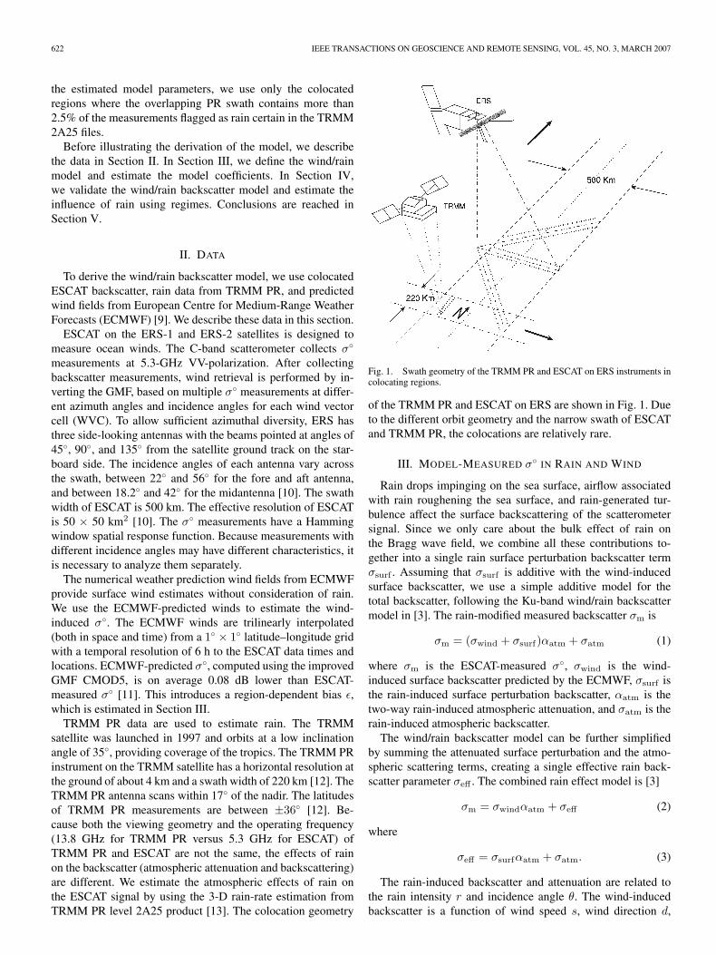
TRMM PR data are used to estimate rain. The TRMMsatellite was launched in 1997 and orbits at a low inclinationangle of 35◦, providing coverage of the tropics. The TRMM PRinstrument on the TRMM satellite has a horizontal resolution atthe ground of about 4 km and a swath width of 220 km [12]. TheTRMM PR antenna scans within 17◦ of the nadir. The latitudesof TRMM PR measurements are between ±36◦ [12]. Be-cause both the viewing geometry and the operating frequency(13.8 GHz for TRMM PR versus 5.3 GHz for ESCAT) ofTRMM PR and ESCAT are not the same, the effects of rainon the backscatter (atmospheric attenuation and backscattering)are different. We estimate the atmospheric effects of rain onthe ESCAT signal by using the 3-D rain-rate estimation fromTRMM PR level 2A25 product [13]. The colocation geometry

Fig. 1. Swath geometry of the TRMM PR and ESCAT on ERS instruments incolocating regions.

of the TRMM PR and ESCAT on ERS are shown in Fig. 1. Dueto the different orbit geometry and the narrow swath of ESCATand TRMM PR, the colocations are relatively rare.

III. MODEL-MEASURED σ◦ IN RAIN AND WIND

Rain drops impinging on the sea surface, airflow associatedwith rain roughening the sea surface, and rain-generated tur-bulence affect the surface backscattering of the scatterometersignal. Since we only care about the bulk effect of rain onthe Bragg wave field, we combine all these contributions to-gether into a single rain surface perturbation backscatter termσsurf . Assuming that σsurf is additive with the wind-inducedsurface backscatter, we use a simple additive model for thetotal backscatter, following the Ku-band wind/rain backscattermodel in [3]. The rain-modified measured backscatter σm is

σm = (σwind + σsurf)αatm + σatm (1)

where σm is the ESCAT-measured σ◦, σwind is the wind-induced surface backscatter predicted by the ECMWF, σsurf isthe rain-induced surface perturbation backscatter, αatm is thetwo-way rain-induced atmospheric attenuation, and σatm is therain-induced atmospheric backscatter.

The wind/rain backscatter model can be further simplifiedby summing the attenuated surface perturbation and the atmo-spheric scattering terms, creating a single effective rain back-scatter parameter σeff . The combined rain effect model is [3]

σm = σwindαatm + σeff (2)

where

σeff = σsurfαatm + σatm. (3)

The rain-induced backscatter and attenuation are related tothe rain intensity r and incidence angle θ. The wind-inducedbackscatter is a function of wind speed s, wind direction d,

NIE AND LONG: C-BAND WIND/RAIN BACKSCATTER MODEL 623

azimuth angle χ, and incidence angle. Thus, the total backscat-ter σm can be expressed as a function F of these parameters

σm = F (r, s, d, χ, θ). (4)

There are two metrics for rain intensity: integrated rain rate(kilometers per millimeter per hour) and surface rain rate (mil-limeters per hour). Because the rain is not uniformly distributedalong the slant path, these two metrics are nonlinearly related.In the Ku-band wind/rain backscatter model, integrated rain rateis used as the metric [3], since contributions of the rain-inducedsurface backscatter and the rain-induced atmospheric backscat-ter are comparable. For the C-band model, the rain-inducedsurface backscatter dominates the rain-generated backscatter,and thus, the surface rain rate (millimeters per hour) is selectedas the rain intensity metric. Also, since the beam of TRMM PRand ESCAT only overlaps on the ocean surface, using surfacerain rate is expected to introduce smaller errors than usingintegrated rain rate.

Because the spatial response function gain is not uniformover the ESCAT footprint, the contribution of rainfall varieswith the location in the footprint. Thus, the ESCAT-observedsurface rain is a weighted average of the surface rain. We definethe weighted-averaging function as

PESCAT =∑N

i=1 G(i)PPR(i)∑Ni=1 G(i)

(5)

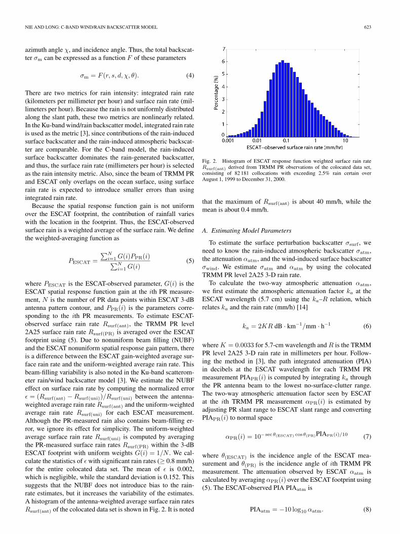
where PESCAT is the ESCAT-observed parameter, G(i) is theESCAT spatial response function gain at the ith PR measure-ment, N is the number of PR data points within ESCAT 3-dBantenna pattern contour, and PPR(i) is the parameters corre-sponding to the ith PR measurements. To estimate ESCAT-observed surface rain rate Rsurf(ant), the TRMM PR level2A25 surface rain rate Rsurf(PR) is averaged over the ESCATfootprint using (5). Due to nonuniform beam filling (NUBF)and the ESCAT nonuniform spatial response gain pattern, thereis a difference between the ESCAT gain-weighted average sur-face rain rate and the uniform-weighted average rain rate. Thisbeam-filling variability is also noted in the Ku-band scatterom-eter rain/wind backscatter model [3]. We estimate the NUBFeffect on surface rain rate by computing the normalized errorε = (Rsurf(ant) − Rsurf(uni))/Rsurf(uni) between the antenna-weighted average rain rate Rsurf(ant) and the uniform-weightedaverage rain rate Rsurf(uni) for each ESCAT measurement.Although the PR-measured rain also contains beam-filling er-ror, we ignore its effect for simplicity. The uniform-weightedaverage surface rain rate Rsurf(uni) is computed by averagingthe PR-measured surface rain rates Rsurf(PR) within the 3-dBESCAT footprint with uniform weights G(i) = 1/N . We cal-culate the statistics of ε with significant rain rates (≥ 0.8 mm/h)for the entire colocated data set. The mean of ε is 0.002,which is negligible, while the standard deviation is 0.152. Thissuggests that the NUBF does not introduce bias to the rain-rate estimates, but it increases the variability of the estimates.A histogram of the antenna-weighted average surface rain ratesRsurf(ant) of the colocated data set is shown in Fig. 2. It is noted

Fig. 2. Histogram of ESCAT response function weighted surface rain rateRsurf(ant) derived from TRMM PR observations of the colocated data set,consisting of 82 181 collocations with exceeding 2.5% rain certain overAugust 1, 1999 to December 31, 2000.

that the maximum of Rsurf(ant) is about 40 mm/h, while themean is about 0.4 mm/h.

A. Estimating Model Parameters

To estimate the surface perturbation backscatter σsurf , weneed to know the rain-induced atmospheric backscatter σatm,the attenuation αatm, and the wind-induced surface backscatterσwind. We estimate σatm and αatm by using the colocatedTRMM PR level 2A25 3-D rain rate.

To calculate the two-way atmospheric attenuation αatm,we first estimate the atmospheric attenuation factor ka at theESCAT wavelength (5.7 cm) using the ka–R relation, whichrelates ka and the rain rate (mm/h) [14]

ka = 2KR dB · km−1/mm · h−1 (6)

where K = 0.0033 for 5.7-cm wavelength and R is the TRMMPR level 2A25 3-D rain rate in millimeters per hour. Follow-ing the method in [3], the path integrated attenuation (PIA)in decibels at the ESCAT wavelength for each TRMM PRmeasurement PIAPR(i) is computed by integrating ka throughthe PR antenna beam to the lowest no-surface-clutter range.The two-way atmospheric attenuation factor seen by ESCATat the ith TRMM PR measurement αPR(i) is estimated byadjusting PR slant range to ESCAT slant range and convertingPIAPR(i) to normal space

αPR(i) = 10− sec θ(ESCAT) cos θ(PR)PIAPR(i)/10 (7)

where θ(ESCAT) is the incidence angle of the ESCAT mea-surement and θ(PR) is the incidence angle of ith TRMM PRmeasurement. The attenuation observed by ESCAT αatm iscalculated by averaging αPR(i) over the ESCAT footprint using(5). The ESCAT-observed PIA PIAatm is

PIAatm = −10 log10 αatm. (8)


Fig. 3. Mean biases between ECMWF-predicted σ◦ and ERS scatterometer-measured σ◦ for fore, mid, and aft antennas at different cross-swath WVC positionsand different wind-speed bins.

ESCAT atmospheric backscatter (σatm) is estimated by thefollowing procedure. First, the effective reflectivity of theatmospheric rain (Ze) is calculated by the Z–R relation[14], [15]

Ze = ARb mm6/m3 (9)

where R is the TRMM PR level 2A25 3-D rain rate (millimetersper hour). The values of A and b depend on the type ofrain. We assume typical stratiform rain value A = 210 andb = 1.6 [14] in this paper. The volume backscattering coeffi-cient without atmospheric attenuation σvc(i) can be computedfrom [16]

σvc(i) = 10−10π5

λ4◦|Kw|2Ze m−1 (10)

where λ◦ = 5.7 cm is the wavelength of ESCAT and |Kw|2 isa function of the wavelength λ◦ and the physical temperatureof the material. Kw is assumed to be 0.93 in this paper.The quantity σvc represents physically the backscattering crosssection (square meters) per unit volume (cubic meters).

By following the method in [3], the volume backscatter crosssection observed by the ESCAT is adjusted by the ESCAT-observed two-way atmospheric attenuation factor. The totalatmospheric rain backscatter observed by the ESCAT at eachTRMM PR measurement σPR(i) is then calculated by inte-grating the adjusted volume backscatter cross section throughthe PR antenna beam to the lowest no-surf-clutter range. TheESCAT-observed atmospheric backscatter σatm is calculated byaveraging σPR(i) using (5).

The wind-induced surface backscatter σwind is estimatedfrom colocated winds from ECMWF winds. As mentioned inSection II, the ECMWF wind fields are interpolated in time andspace to the center of each ESCAT measurement using cubicspline interpolation of the zonal and meridional componentsof the wind. We compute the speed and direction of the windin meteorological convention and calculate the σ◦ for threeantennas of each ESCAT WVC through ERS GMF (CMOD5)

σwind(ECMWF) = CMOD5(s, d, χ, θ) (11)

where the definition of the inputs of CMOD5 is the same asin (4). The wind-induced backscatter σwind(ECMWF) predictedby ECMWF has a bias ε introduced by prediction errors. Sincethe ECMWF wind fields are interpolated from low resolution toESCAT resolution, the bias of ECMWF wind fields is spatiallycorrelated in an ESCAT swath. To reduce the effect of the spa-tial correlation and contamination of rain on the measurements,we use a large data set (from January 1, 2000 to December 31,2000) to estimate the ECMWF/ESCAT bias. The bias varieswith incidence angle and antenna look direction, and it maychange with wind speed and geophysical locations. Thus, weestimate ε for a specific look direction and incidence angle foreach wind-speed bin by making a nonparametric estimate ofε = σm(ESCAT) − σwind(ECMWF) as a function of wind speedat evenly spaced wind-speed bins (from 0–20 m/s with a binwidth of 1 m/s) by using an Epanechnikov kernel with abandwidth of 3 m/s in wind speed. Only the colocated ECMWFand ESCAT data between latitude −40◦ and 40◦ are used toestimate the bias. Fig. 3 shows the mean of ε for fore, mid,and aft antennas at different cross-swath WVC positions anddifferent wind-speed bins. Note that the bias is positive at lowwind speed and is negative at high wind speed. The standarddeviations of the bias ε for three antennas are less than 0.0074for incidence angles greater than 40◦. The estimate of wind-induced backscatter σwind is then represented by ECMWF-predicted wind-induced backscatter σwind(ECMWF) and bias ε

σwind = σwind(ECMWF) + ε. (12)

Based on the above parameters, we estimate the surfaceperturbation backscatter σsurf by

σsurf = α−1atm(σm − σatm) − (σwind(ECMWF) + ε). (13)

B. Selecting Model Function and EstimatingModel Coefficients

We seek an empirical model function for (4). Power law(linear or quadratic log-log) models are sufficient to relate thethree parameters with rain rate in Ku-band wind/rain backscat-ter model [3]. Similar functional forms work well at C-band.


Thus, αatm, σatm, and σsurf for a specific incidence angle θcan be expressed as polynomial functions of rain rate

10 log10 (PIAatm(θ)) = 10 log10 (−10 log10 αatm(θ))

≈ fa(RdB) =N∑

n=0

xa(n)RndB (14)

10 log10 (σatm(θ)) ≈ fr(RdB) =N∑

n=0

xr(n)RndB (15)

10 log10 (σsurf(θ)) ≈ fsr(RdB) =N∑

n=0

xsr(n)RndB (16)

where RdB = 10 log10(Rsurf(ant)), xa(n), xr(n), and xsr(n)are the corresponding model coefficients. N = 1 for the lin-ear model, and N = 2 for the quadratic model. Because theestimate of σsurf is relatively noisy and may be negative, wefirst make a nonparametric estimate of σsurf as a functionof RdB at regular logarithmically spaced rain-rate bins usingan Epanechnikov kernel [17] with a 3-dB bandwidth in RdB.Then, we estimate the model coefficients xsr(n) for the lin-ear/quadratic model using a robust linear least squares fit. Weuse a similar method in estimating xa(n) and xr(n). Since theatmospheric parameters and surface perturbation backscatterare uncorrelated with the azimuth look direction of the antenna,we combine the data from all antennas during the coefficientestimation. To ensure sufficient data for each model fit, we usean incidence-angle bin size approximately equal to 4◦. Becausethe incidence angles of the ESCAT measurements are notuniformly distributed, the bin size is slightly increased wheremeasurements at the incidence-angle range are more rare.

In the analysis, we observe that for incidence angles less than30◦, the surface rain perturbation is not a monotonic function ofsurface rain rate. It cannot adequately be modeled by a linearor quadratic model. A hypothesis for the reason is that thecontributions of ring waves and upper surface turbulence arecomparable under such conditions. For incidence angles greaterthan 30◦, the surface rain perturbation is monotonically increas-ing with surface rain rate, suggesting that the contribution ofring waves dominates the surface effects of rain. We note thatthe Bragg wavelength of ESCAT at incidence angles higherthan 30◦ is shorter than 5.8 cm, which is close to the wave-length condition mentioned previously. For incidence anglesbetween 30◦ and 40◦, the variance of the estimation of σsurf isrelatively large, which makes the model coefficients unreliable.Thus, in this paper, we only describe the model coefficients forincidence angles greater than 40◦. It is noted that due to theinhomogeneity of rain events in an ESCAT footprint, only thetotal surface effect of rain in the backscatter measurements canbe described by the model.

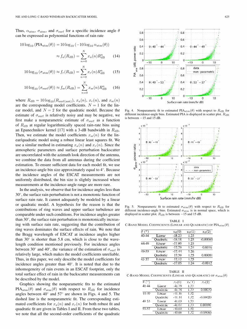
Graphics showing the nonparametric fits to the estimatedPIAatm(θ) and σatm(θ) with respect to RdB for incidenceangles between 40◦ and 57◦ are shown in Figs. 4 and 5. Thedashed line is the nonparametric fit. The corresponding esti-mated coefficients for xa(n) and xr(n) for both robust fit andquadratic fit are given in Tables I and II. From these two tables,we note that all the second-order coefficients of the quadratic

Fig. 4. Nonparameric fit to estimated PIAatm(θ) with respect to RdB fordifferent incidence-angle bins. Estimated PIA is displayed in scatter plot. RdB

is between −15 and 15 dB.

Fig. 5. Nonparameric fit to estimated σatm(θ) with respect to RdB fordifferent incidence-angle bins. Estimated σatm is in normal space, which isdisplayed in scatter plot. RdB is between −15 and 15 dB.

TABLE IC-BAND MODEL COEFFICIENTS (LINEAR AND QUADRATIC) OF PIAatm(θ)

TABLE IIC-BAND MODEL COEFFICIENTS (LINEAR AND QUADRATIC) OF σatm(θ)


Fig. 6. xsr(n) for the quadratic model as a function of the rain backscattercalibration parameter γ for different incidence-angle ranges.

model are negligibly small, suggesting that PIAatm(θ) andσatm(θ) are almost a linear function of surface rain rate in log-log space.

In the derivation of σsurf(θ), error is introduced by severalsources. One of them is the prediction error of the ECMWFpredicted wind-induced backscatter σwind. The procedure forestimating αatm and σatm from the TRMM PR level 2A253-D rain rate introduces additional errors due to the error of theempirical model functions, NUBF, and the temporal and spatialmismatch of ESCAT and TRMM PR measurements. We donot analyze all these errors in detail here. Instead, we evaluatethe sensitivity of σsurf(θ) to the error introduced by σatm. Weadopt the combined rain model of (2) to reduce the influenceof the error.

To evaluate the sensitivity of σsurf(θ) to σatm, followingthe study in [3], we introduce a variable calibration parameterγ to (13)

σsurf = α−1atm(σm − γσatm) − (

σwind(ECMWF) + ε). (17)

Using the method described above, we calculate the linear/quadratic model coefficients of σsurf(θ) for each γ between 0and 3.2 with a step of 0.1. When γ is greater than 3.2, σsurf(θ)may become negative. We pick the optimum γ by defining aleast squares objective function f(γ) with respect to γ

f(γ) =∑

i

(σim − σi

m(model)(γ))2

(18)

where i is the ith data in the data set and σm(model)(γ) isthe σ◦ calculated with the quadratic model coefficients withrespect to the corresponding γ. The value of γ that minimizesf(γ) is the optimum value γopt. For all the measurements withincidence angles between 40◦ and 57◦, γopt = 1.2, suggestingthat the estimates of σatm are slightly underestimated. Theestimated coefficients of σsurf(θ) are plotted as a function ofthe calibration parameter γ for different incidence-angle bins inFig. 6. We note that none of the three terms are particularlysensitive to the value of γ, suggesting that the influence ofthe σatm-induced error is insignificant as expected. We list thevalues of xsr(n) corresponding to γopt in Table III. Comparedwith the counterparts in Table II, it is noted that the constantterm of σsurf(θ) is significantly higher than the constant term ofσatm(θ), while the linear and quadratic terms of σsurf(θ) are onthe same order of magnitude as the linear and quadratic termsof σatm(θ).

TABLE IIIMODEL COEFFICIENTS OF SURFACE PERTURBATION

BACKSCATTER σsurf(θ)

Fig. 7. Ratio of the attenuated surface perturbation αatmσsurf(θ) to thecalibrated atmospheric rain backscatter γσatm for different γ in the range of0.1–3.2 with a step of 0.1 separately plotted as a function of rain rate for severalincidence-angle ranges. Dashed line corresponds to γopt.

To further compare the contribution of the surface pertur-bation and the atmospheric backscatter, we compute the ra-tio of the attenuated surface perturbation αatmσsurf(θ) to thecalibrated atmospheric rain backscatter γσatm(θ) with respectto RdB for different incidence-angle bins, which is shown inFig. 7. For γopt, the ratio αatmσsurf/γσatm(θ) for different θis always greater than three, suggesting that the surface rainbackscatter always dominates the total rain-induced backscatter(but not necessarily the total backscatter).

It is noted that we only care about the total effect of rain inwind retrieval. The corresponding power law model of σeff is

10 log10 (σeff(θ)) ≈ fe(RdB) =N∑

n=0

xe(n)RndB. (19)

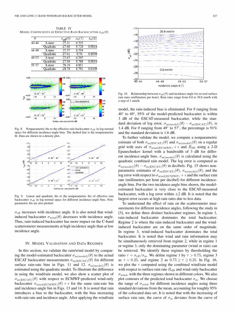
The coefficients of xe(n) are calculated using the same methodmentioned before, shown in Table IV, and plotted in Fig. 8. Theestimated σeff(θ) is shown in the density plot. The dashed lineis the nonparametric fit. Fig. 9 shows the nonparametric fit andlinear/quadratic fits in log-log space.

We further investigate the relationship between σeff(θ) andincidence angle θ by plotting the σeff(θ) with respect to θ for aspecific surface rain rate in Fig. 10. We use the quadratic modelcoefficients to estimate σeff(θ) for θ between 40◦ and 57◦.At a low rain rate, the magnitude of σeff generally decreaseswith incidence angle. At a moderate rain rate, the σeff almostremains constant for all incidence angles. At a heavy rain rate,


TABLE IVMODEL COEFFICIENTS OF EFFECTIVE RAIN BACKSCATTER σeff(θ)

Fig. 8. Nonparametric fits to the effective rain backscatter σeff in log-normalspace for different incidence-angle bins. The dashed line is the nonparametricfit. Data are shown in a density plot.

Fig. 9. Linear and quadratic fits to the nonparametric fits of effective rainbackscatter σeff in log-normal space for different incidence-angle bins. Non-parametric fits are also plotted.

σeff increases with incidence angle. It is also noted that wind-induced backscatter σwind(θ) decreases with incidence angle.Thus, rain-induced backscatter has more impact on the C-bandscatterometer measurements at high incidence angle than at lowincidence angle.

IV. MODEL VALIDATION AND DATA REGIMES

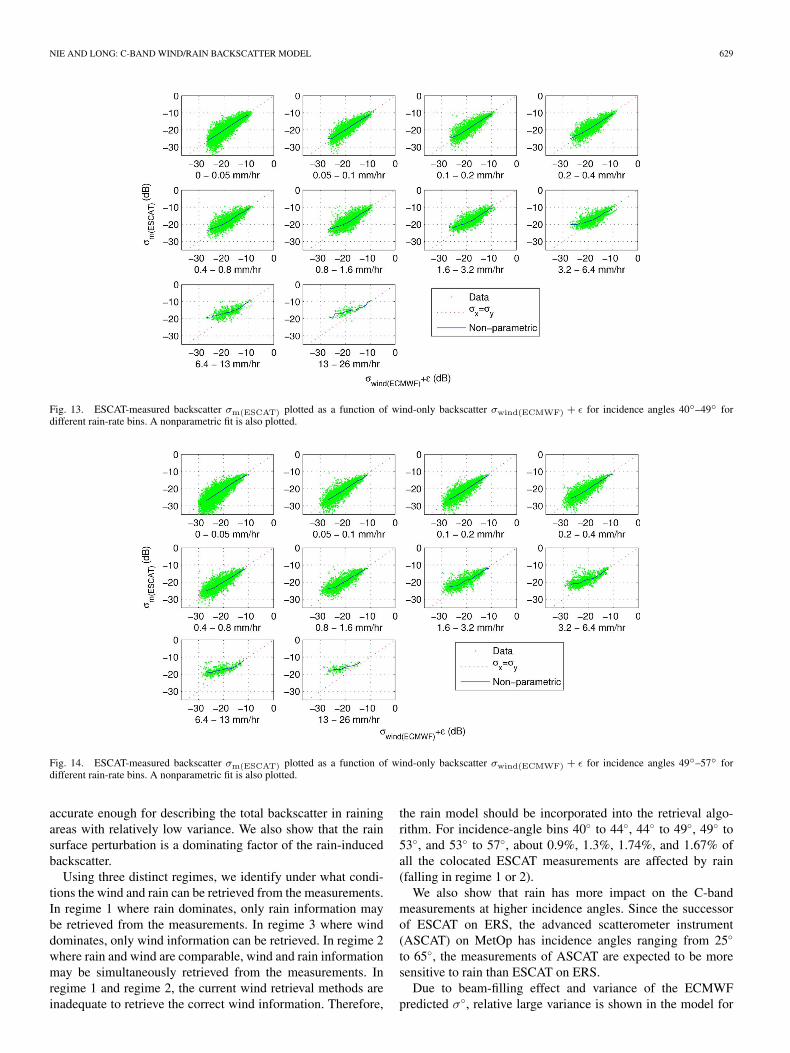
In this section, we validate the rain/wind model by compar-ing the model-estimated backscatter σm(model)(θ) to the actualESCAT backscatter measurements σm(ESCAT)(θ) for differentsurface rain-rate bins in Figs. 11 and 12. σm(model)(θ) isestimated using the quadratic model. To illustrate the differencein using the wind/rain model, we also show a scatter plot ofσm(ESCAT)(θ) with respect to ECMWF-predicted wind-onlybackscatter σwind(ECMWF)(θ) + ε for the same rain-rate binand incidence-angle bin in Figs. 13 and 14. It is noted that rainintroduces a bias to the backscatter, with the bias increasingwith rain rate and incidence angle. After applying the wind/rain

Fig. 10. Relationship between σeff(θ) and incidence angle for several surfacerain rates (millimeters per hour). Rain rates range from 0.8 to 30.8 mm/h witha step of 1 mm/h.

model, the rain-induced bias is eliminated. For θ ranging from40◦ to 49◦, 95% of the model-predicted backscatter is within3 dB of the ESCAT-measured backscatter, while the stan-dard deviation of log error, σm(model)(θ) − σm(ESCAT)(θ), is1.4 dB. For θ ranging from 49◦ to 57◦, the percentage is 91%and the standard deviation is 1.6 dB.

To further validate the model, we compute a nonparametricestimate of both σm(ESCAT)(θ) and σm(model)(θ) on a regulargrid with axes of σwind(ECMWF) + ε and RdB using a 2-DEpanechnikov kernel with a bandwidth of 3 dB for differ-ent incidence-angle bins. σm(model)(θ) is calculated using thequadratic combined rain model. The log error is computed asσm(model)(θ) − σm(ESCAT)(θ) in decibels. Fig. 15 shows non-parametric estimates of σm(ESCAT)(θ), σm(model)(θ), and thelog error with respect to σwind(ECMWF) + ε and the surface rainrate (millimeters per hour per decibel) for different incidence-angle bins. For the two incidence-angle bins shown, the model-estimated backscatter is very close to the ESCAT-measuredbackscatter, with a log error within ±2 dB. It is noted that thelargest error occurs at high rain rates due to less data.

To understand the effect of rain on the scatterometer mea-surements for different incidence angles, following the study in[3], we define three distinct backscatter regimes. In regime 1,rain-induced backscatter dominates the total backscatter.Regime 2 is where the rain-induced backscatter and the wind-induced backscatter are on the same order of magnitude.In regime 3, wind-induced backscatter dominates the totalbackscatter. It is noted that wind and rain information maybe simultaneously retrieved from regime 2, while in regime 1or regime 3, only the dominating parameter (wind or rain) canbe retrieved. We identify these regimes by thresholding theratio τ = σeff/σm. We define regime 1 by τ > 0.75, regime 3as τ < 0.25, and regime 2 as 0.75 ≥ τ ≥ 0.25. In Fig. 16,we plot the τ computed using the combined wind/rain modelwith respect to surface rain rate RdB and wind-only backscatterσwind, with the three regimes shown in different colors. We alsoplot contours of the predicted total backscatter σm. We choosethe range of σwind for different incidence angles using threestandard deviations from the mean, accounting for roughly 95%of the colocated data set. It is noted that with the increasing ofsurface rain rate, the curve of σm deviates from the curve of


Fig. 11. ESCAT-measured backscatter σm(ESCAT) plotted as a function of model-estimated backscatter σm(model) with the quadratic model for incidenceangles 40◦–49◦ for different rain-rate bins. A nonparametric fit is also plotted.

Fig. 12. ESCAT-measured backscatter σm(ESCAT) plotted as a function of model-estimated backscatter σm(model) with the quadratic model for incidenceangles 49◦–57◦ for different rain-rate bins. A nonparametric fit is also plotted.

σwind. As the incidence angle increases, the area of regime 1reduces while the area of regime 3 increases, suggesting thatrain has more significant impact on the ESCAT measurementsat higher incidence angles.

We further investigate this by computing the percentage ofcolocated measurements falling in each regime with significantrain (≥ 0.8 mm/h) and ECMWF wind speed greater than2 m/s, listed in Table V. It is noted that about 3% of allthe colocated ESCAT measurements observe significant rain(≥ 0.8 mm/h). To investigate the relationship between the dataregimes, wind speed, and rain rate, we plot mean τ with respectto the ECMWF-predicted wind speed and average surface rainrate (millimeters per hour) for all the colocated measurementswith significant rain (≥ 0.8 mm/h) and ECMWF wind speedgreater than 2 m/s in Fig. 17, with a bin width of 4 m/s for wind

speed and a bin width of 4 mm/h for surface rain rate. It is notedthat regime 1 (τ > 0.75) mostly happens at low wind speedand high rain conditions, suggesting that rain has a significantimpact on the total backscatter in such conditions.

V. CONCLUSION

With the confirmed existence of rain surface perturbation byrecent studies, the rain effect on C-band scatterometer measure-ments needs to be reevaluated. By using colocated TRMM PR,ESCAT on ERS, and ECMWF data, we develop and evaluatea simple low-order wind/rain backscatter model which inputssurface rain rate, incidence angle, wind speed, wind direction,and azimuth angle. By applying the model to the colocateddata set, we demonstrate that the wind/rain backscatter model is


Fig. 13. ESCAT-measured backscatter σm(ESCAT) plotted as a function of wind-only backscatter σwind(ECMWF) + ε for incidence angles 40◦–49◦ fordifferent rain-rate bins. A nonparametric fit is also plotted.

Fig. 14. ESCAT-measured backscatter σm(ESCAT) plotted as a function of wind-only backscatter σwind(ECMWF) + ε for incidence angles 49◦–57◦ fordifferent rain-rate bins. A nonparametric fit is also plotted.

accurate enough for describing the total backscatter in rainingareas with relatively low variance. We also show that the rainsurface perturbation is a dominating factor of the rain-inducedbackscatter.

Using three distinct regimes, we identify under what condi-tions the wind and rain can be retrieved from the measurements.In regime 1 where rain dominates, only rain information maybe retrieved from the measurements. In regime 3 where winddominates, only wind information can be retrieved. In regime 2where rain and wind are comparable, wind and rain informationmay be simultaneously retrieved from the measurements. Inregime 1 and regime 2, the current wind retrieval methods areinadequate to retrieve the correct wind information. Therefore,

the rain model should be incorporated into the retrieval algo-rithm. For incidence-angle bins 40◦ to 44◦, 44◦ to 49◦, 49◦ to53◦, and 53◦ to 57◦, about 0.9%, 1.3%, 1.74%, and 1.67% ofall the colocated ESCAT measurements are affected by rain(falling in regime 1 or 2).

We also show that rain has more impact on the C-bandmeasurements at higher incidence angles. Since the successorof ESCAT on ERS, the advanced scatterometer instrument(ASCAT) on MetOp has incidence angles ranging from 25◦

to 65◦, the measurements of ASCAT are expected to be moresensitive to rain than ESCAT on ERS.

Due to beam-filling effect and variance of the ECMWFpredicted σ◦, relative large variance is shown in the model for


Fig. 15. Nonparametric estimates of σm(ESCAT)(θ), σm(model)(θ), and the difference are plotted with respect to σwind(ECMWF) + ε and surface rain rateR(mm/h · dB) for incidence angles in range of (a) 40◦–49◦ and (b) 49◦–57◦.

Fig. 16. Backscatter regimes for ESCAT as a function of rain rate andeffective wind backscatter for several incidence angles. Also plotted is a contourplot of the combined rain effect model for σm (solid lines) and σwind (dottedlines).

TABLE VPERCENTAGE FALLING IN EACH REGIME OF COLOCATED

MEASUREMENTS WITH SIGNIFICANT RAIN (≥ 0.8 mm/h)AND ECMWF WIND SPEED GREATER THAN 2 m/s.

THIS REPRESENTS 3% OF THE TOTAL DATA

Fig. 17. Mean σeff/σm with respect to ECMWF-predicted wind speed andTRMM PR-measured surface rain rate for different incidence-angle bins. Thewind speed ranges from 2–22 m/s with a bin width of 4 m/s. The surface rainrate ranges from 0.8–20.8 mm/h with a bin width of 4 mm/h.

low rain data. But, the majority of the data (95% for 40◦ to49◦ and 91% for 49◦ to 57◦) lie within 3 dB of the model.This illustrates how well the model performs. In fact, ESCATretrieved wind vectors are mainly affected by mid-to-heavy rainat high incidence angles. The model is expected to retrieve rainrate and improve the retrieved wind vector in such situations. Afollowing paper will explore this in great detail.


ACKNOWLEDGMENT

The authors would like to thank R. Halterman for his assis-tance in colocating the ESCAT/TRMM PR data.

REFERENCES

[1] I. I. Lin, D. Kasilingam, W. Alpers, T. K. Lim, H. Lim, andV. Khoo, “A quantitative study of tropical rain cells from ERS SARimagery,” in Proc. Int. Geosci. and Remote Sens. Symp., Singapore, 1997,pp. 1527–1529.

[2] D. Kasilingam, I. I. Lin, H. Lim, V. Khoo, W. Alpers, and T. K. Lim,“Investigation of tropical rain cells with ERS SAR imagery and ground-based weather radar,” in Proc. 3rd ERS Symp., 1997, pp. 1603–1608.

[3] D. W. Draper and D. G. Long, “Evaluating the effect of rain on Sea-Winds scatterometer measurements,” J. Geophys. Res., vol. 109, no. C12,pp. C02005.1–C02005.12, Feb. 2004.

[4] N. Braun, M. Gade, and P. A. Lange, “Radar backscattering measurementsof artificial rain impinging on a water surface at different wind speeds,”in Proc. Int. Geosci. and Remote Sens. Symp., Hamburg, Germany, 1999,pp. 1963–1965.

[5] C. Melsheimer, W. Alpers, and M. Gade, “Simultaneous observations ofrain cells over the ocean by the synthetic aperture radar aboard the ERSsatellites and by surface-based weather radars,” J. Geophys. Res., vol. 106,no. C3, pp. 4665–4677, Mar. 2001.

[6] M. H. Freilich and R. S. Dunbar, “Derivation of satellite windmodel functions using operational surface wind analyses: An altime-ter example,” J. Geophys. Res., vol. 98, no. C8, pp. 14 633–14 649,Aug. 1993.

[7] L. F. Bliven, P. W. Sobieski, and C. Craeye, “Rain generated ring-waves:Measurements and modeling for remote sensing,” Int. J. Remote Sens.,vol. 18, no. 1, pp. 221–228, Jan. 1997.

[8] L. F. Bliven, J. P. Giovanangeli, and G. Norcross, “Scatterometer direc-tional response during rain,” in Proc. IEEE Int. Geosci. Remote Sens.Symp., 1989, pp. 1887–1890.

[9] A. Persson and F. Grazzini, User Guide to ECMWF Forecast Prod-ucts. Reading, U.K.: Eur. Centre Medium Range Weather Forecasts,2005.

[10] E. Attema, “The Active Microwave Instrument onboard the ERS-1 satel-lite,” Proc. IEEE, vol. 79, no. 6, pp. 791–799, Jun. 1991.

[11] H. Hersbach, “CMOD5—An improved geophysical model function forERS C-band scatterometry,” ECMWF, Reading, U.K., ECMWF Tech.Memo. No. 395, 2003.

[12] T. Kozu, T. Kawanishi, H. Kuroiwa et al., “Development of precipita-tion radar on-board the Tropical Rainfall Measuring Mission (TRMM)satellite,” IEEE Trans. Geosci. Remote Sens., vol. 39, no. 1, pp. 102–116,Jan. 2001.

[13] T. Iguchi, T. Kozu, R. Meneghini, J. Awaka, and K. Okamoto, “Rain pro-filing algorithm for the TRMM Precipitation Radar,” J. Appl. Meteorol.,vol. 39, no. 12, pp. 2038–2052, Dec. 2000.

[14] L. J. Battan, Radar Observation of the Atmosphere. Chicago, IL: Univ.Chicago Press, 1973.

[15] R. J. Doviak and D. S. Zrnic, Doppler Radar and Weather Observations.San Diego, CA: Academic, 1984.

[16] F. T. Ulaby, R. K. Moore, and A. K. Fung, Microwave Remote Sensing:Active and Passive, vol. II. Reading, MA: Artech House, 1982.

[17] M. P. Wand and M. C. Jones, Kernel Smoothing. London, U.K.:Chapman & Hall, 1995.

Congling Nie (S’06) received the B.S. degree inelectrical engineering from the South China Uni-versity of Technology, Guangzhou, China, in 1995.He is currently working toward the Ph.D. degree inelectrical engineering at Brigham Young University(BYU), Provo, UT.

From 1995 to 2003, he was with the Meteorolog-ical Center of Central and South China Air TrafficManagement Bureau, where he developed weatherradar applications for air traffic control. He joined theMicrowave Earth Remote Sensing Research Group

at BYU, Provo, UT, in 2003. His current research interests include rain effectson microwave backscatter from ocean surfaces and scatterometer wind retrieval.

David G. Long (S’80–M’82–SM’98) received thePh.D. degree in electrical engineering from the Uni-versity of Southern California, Los Angeles, in 1989.

From 1983 to 1990, he worked with NASA’s JetPropulsion Laboratory (JPL) where he developedadvanced radar remote sensing systems. While withJPL, he was the Project Engineer on the NASA Scat-terometer (NSCAT) project, which flew from 1996to 1997. He also managed the SCANSCAT project,the precursor to SeaWinds, which was launched in1999 and 2002. He is currently a Professor with the

Electrical and Computer Engineering Department at Brigham Young University(BYU), Provo, UT, where he teaches upper division and graduate courses incommunications, microwave remote sensing, radar, and signal processing. Heis the Director with the BYU Center for remote sensing. He is the PrincipalInvestigator on several NASA-sponsored research projects in remote sensing.He has numerous publications in signal processing and radar scatterometry.His research interests include microwave remote sensing, radar theory, space-based sensing, estimation theory, signal processing, and mesoscale atmosphericdynamics. He has over 275 publications.

Dr. Long has received the NASA Certificate of Recognition several times.He is an Associate Editor of the IEEE GEOSCIENCE AND REMOTE SENSING

LETTERS.

a c-band wind/rain backscatter model

Documents