a broadband vhf-l band cavity-backed slot ... final technical report may 2005 a broadband vhf-l band...
TRANSCRIPT

AFRL-IF-RS-TR-2005-169 Final Technical Report May 2005 A BROADBAND VHF-L BAND CAVITY-BACKED SLOT SPIRAL ANTENNA University of Michigan
APPROVED FOR PUBLIC RELEASE; DISTRIBUTION UNLIMITED.
AIR FORCE RESEARCH LABORATORY INFORMATION DIRECTORATE
ROME RESEARCH SITE ROME, NEW YORK
STINFO FINAL REPORT This report has been reviewed by the Air Force Research Laboratory, Information Directorate, Public Affairs Office (IFOIPA) and is releasable to the National Technical Information Service (NTIS). At NTIS it will be releasable to the general public, including foreign nations. AFRL-IF-RS-TR-2005-169 has been reviewed and is approved for publication APPROVED: /s/
STEPHEN REICHHART Project Engineer
FOR THE DIRECTOR: /s/
WARREN H. DEBANY, JR., Technical Advisor Information Grid Division Information Directorate

REPORT DOCUMENTATION PAGE Form Approved
OMB No. 074-0188 Public reporting burden for this collection of information is estimated to average 1 hour per response, including the time for reviewing instructions, searching existing data sources, gathering and maintaining the data needed, and completing and reviewing this collection of information. Send comments regarding this burden estimate or any other aspect of this collection of information, including suggestions for reducing this burden to Washington Headquarters Services, Directorate for Information Operations and Reports, 1215 Jefferson Davis Highway, Suite 1204, Arlington, VA 22202-4302, and to the Office of Management and Budget, Paperwork Reduction Project (0704-0188), Washington, DC 20503 1. AGENCY USE ONLY (Leave blank)
2. REPORT DATEMAY 2005
3. REPORT TYPE AND DATES COVERED Final Feb 01 – Nov 04
4. TITLE AND SUBTITLE A BROADBAND VHF-L BAND CAVITY-BACKED SLOT SPIRAL ANTENNA
6. AUTHOR(S) John L. Volakis
5. FUNDING NUMBERS C - F30602-98-C-0233 PE - 63617F PR - 2317 TA - 08 WU - 04
7. PERFORMING ORGANIZATION NAME(S) AND ADDRESS(ES) University of Michigan
Ann Arbor Michigan
8. PERFORMING ORGANIZATION REPORT NUMBER
N/A
9. SPONSORING / MONITORING AGENCY NAME(S) AND ADDRESS(ES) Air Force Research Laboratory/IFGC 525 Brooks Road Rome New York 13441-4505
10. SPONSORING / MONITORING AGENCY REPORT NUMBER
AFRL-IF-RS-TR-2005-169
11. SUPPLEMENTARY NOTES AFRL Project Engineer: Stephen Reichart/IFGC/(315) 330-3918/ [email protected]
12a. DISTRIBUTION / AVAILABILITY STATEMENT APPROVED FOR PUBLIC RELEASE; DISTRIBUTION UNLIMITED.
12b. DISTRIBUTION CODE
13. ABSTRACT (Maximum 200 Words) Slot spiral antennas offer the possibility for very thin and conformal designs. This report covers the physical characteristic of a cavity-backed slot spiral, as well as the associated infinite balun and termination designs. The report traces through the development and characteristics of a 6” and 18” version of the slot spiral. Simulations and measurements of various cavity-backed spirals are presented and used to optimize the antenna’s computations. Several options for miniaturizing this design using capacitive and inductive loadings are also presented.
15. NUMBER OF PAGES58
14. SUBJECT TERMS Slot Spiral Antenna, Cavity-Backed
16. PRICE CODE
17. SECURITY CLASSIFICATION OF REPORT
UNCLASSIFIED
18. SECURITY CLASSIFICATION OF THIS PAGE
UNCLASSIFIED
19. SECURITY CLASSIFICATION OF ABSTRACT
UNCLASSIFIED
20. LIMITATION OF ABSTRACT
ULNSN 7540-01-280-5500 Standard Form 298 (Rev. 2-89)
Prescribed by ANSI Std. Z39-18 298-102

Table of Contents
INTRODUCTION. ..............................................................................................................1 PAPERS AND PATENTS GENERATED UNDER THIS PROJECT. ..............................2 CONFERENCE PAPERS....................................................................................................3 SLOT SPIRAL ANTENNA DESCRIPTION. ....................................................................4 PHYSICAL PROPERTIES OF THE SLOT SPIRAL.........................................................6 SLOT SPIRAL PERFORMANCE. ...................................................................................10 MINIATURIZATION USING DIELECTRIC LOADING...............................................12 SIX-INCH APERTURE DEVELOPMENT......................................................................17 HF/VHF TO L-BAND DESIGN. ......................................................................................23 PLATFORM PATTERN EVALUATIONS-SIMULATIONS..........................................25 AIRCRAFT MODEL..................................................................................................25 PLATFORM ANALYSIS. .........................................................................................28 FLIGHT TEST DATA.......................................................................................................30 CONCLUSION..................................................................................................................32 REFERENCES. .................................................................................................................33 APPENDIX A: BLURB FROM THE AFRL WEB SITE-MAY 2004 ACCOMPLISHMENTS. ........................................................................34 APPENDIX B: SLOT SPIRAL ANTENNA FLIGHT TEST REPORT BY ROBERT FRENCH..................................................................................................35
i

List of Figures
Figure 1. Bottom of the slot spiral. ......................................................................................4 Figure 2. Top of slot spiral, showing the microstrip balun..................................................5 Figure 3. Cross section of slot spiral showing how the microstrip balun excites the slot spiral at its center .......................................................................................................5 Figure 4: Chip resistor implementation of the slot spiral termination. ................................8 Figure 5: Shunt resistance as a function of position for the slot spiral termination............9 Figure 6: Thick film implementation of the slot spiral termination....................................9 Figure 7. Illustration of simulated antenna grid for comparison with measurements. .....10 Figure 8. Comparison of full scale simulations and measurements of the broadside gain and axial ratios for the 14.5cm antenna aperture shown in Figure 7. .....................11 Figure 9. Measured patterns for the 14.5cm antenna aperture-flat 1.27cm cavity. ..........12 Figure 10. Geometry of considered archimedean spiral antennas. ....................................13 Figure 11. Total electric field over the spiral slot for various substrates, at f=2.2GHz.....14 Figure 12. Magnetic current propagating in the spiral slot for various dielectric constants.........................................................................................................................14 Figure 13. Miniaturization vs. substrate thickness.............................................................16 Figure 14. Phase progression for different superstrate dielectric thickness and dielectric values. .............................................................................................................16 Figure 15. Miniaturization vs. superstrate thickness. ........................................................17 Figure 16. Basic 6” antenna A1: geometry and comparison with the initial Design .............................................................................................................................17 Figure 17. The gain and axial ratio comparisons: the initial antenna vs. A1.....................18 Figure 18. Reducing the effect of TM resonance by cavity loading..................................18 Figure 19. Antenna gain vs. cavity thickness. ...................................................................19 Figure 20. Antenna A2: geometry and comparison with the initial design. ......................19 Figure 21. The gain and axial ratio comparisons: the initial antenna vs. A2.....................20 Figure 22. Antenna A3: geometry and comparison with the initial design. ......................20 Figure 23. The gain and axial ratio comparisons: the initial antenna vs. A3.....................20 Figure 24. Antenna A4: geometry and comparison with the initial design. ......................21 Figure 25. The gain and axial ratio comparisons: the initial antenna vs. A4.....................21 Figure 26. Meanderline antenna A5: geometry and comparison with the initial design. .............................................................................................................................22 Figure 27. The gain and axial ratio comparisons: the initial antenna vs. A5.....................22 Figure 28. The gain variations for various resistive tapers................................................22 Figure 29. Meanderline antenna A6: geometry and comparison with the initial design. ............................................................................................................................23 Figure 30. The gain and axial ratio comparisons: the initial antenna vs. A6.....................23 Figure 31. Geometry of 18” antennas A7 and A8. ............................................................23 Figure 32. Outdoor measurement site at Rome, NY..........................................................24 Figure 33. Broadside gain of 18” antennas........................................................................24
ii

Figure 34. AR of loaded vs. unloaded cavity.....................................................................25 Figure 35. Return loss for 18” antennas.............................................................................25 Figure 36. Unmeshed C-135 model. .................................................................................25 Figure 37. Meshed cockpit from the front and side: 1117 nodes, 259 elements ...............26 Figure 38. Meshed wing section: 9912 nodes, 2441 elements. ........................................27 Figure 39. Meshed tail section: 2485 nodes, 617 elements. .............................................27 Figure 40. Entire C-135 meshed: 13515 nodes, 3317 elements. .......................................28 Figure 41. Antenna above center. .....................................................................................28 Figure 42. Antenna below center. ......................................................................................28 Figure 43. Antenna above plane and in front of tail. .........................................................28 Figure 44. Calculated Patterns at 30MHz and 50Mhz when the antenna is placed on the top and bottom of the aircraft....................................................................................29 Figure 45. Sketch of the C135E serial No. 600372 and a photo of the antenna (with radome at the right) mounting at the aircraft bottom......................................................31
List of Tables
Table 1. Parameters of the substrates employed in the present analysis. ..........................13
iii

1 4
INTRODUCTION Spiral antennas are known for their ability to maintain nearly circular polarization (low axial-ratio radiation patterns) and consistent gain and input impedance over wide bandwidths. It is not therefore surprising that a wide range of applications exist, ranging from military surveillance, ECM, and ECCM to numerous commercial and private uses, including the consolidation of multiple low gain communications antennas on moving vehicles. In particular, there is significant military and commercial interest in extremely broadband antennas that can be conformally mounted on land, air, and sea vehicles. Bandwidths of as much as 100:1 are desired, with frequencies ranging from below 30 MHz to past 6 GHz. To further complicate matters, the aperture size is often limited to significantly less than optimal while still demanding maximum gain and pattern coverage. There are essentially two basic types of broadband spirals in use today. By far, the most common is the wire, or ”printed” spiral, consisting essentially of two long, constant width strips that have been wound around each other to form a (generally planar) spiral. The gaps between the strips are generally of constant width as well, and are usually wider than the strips themselves. The other type of spiral is the complementary spiral, in which the widths of the conductors and the widths of the spaces between them are equal and a function of angle, increasing with distance from the terminals. Complementary spirals are frequently conical in shape rather than planar, and find only very specialized application due to their shape, size, and complexity. For the more typical wire or microstrip spiral antenna, the performance advantages mentioned above come at the price of size and complexity. As mentioned above, antennas of this type may have upwards of 20:1 bandwidth and very consistent gain, polarization, and pattern shape. However, while the antenna's radiating elements may be planar, the feed network and balun structures generally are not, and combine to add weight, depth, and significant complexity to the system. Furthermore, because the spiral antenna has front-to-back symmetry and prefers to radiate bi-directionally, a broadband absorbing cavity is typically used for unidirectional radiation, adding even more depth and weight to the antenna and reducing its gain by at least 3 dB. While some designs integrate the feed and balun into the cavity and reduce the complexity somewhat [1], the absorbing cavity is still at least a quarter-wavelength deep at the lowest frequency of operation, adding significant depth, weight, and cost to the antenna [2]. A new spiral antenna paradigm utilizing slot radiating elements is presented (see Figure 1) that resolves many of the aforementioned shortcomings while generally maintaining or improving overall performance [3, 4, 5, 6, 7, 9]. Spirals of this type are also amenable to techniques, which allow for increased bandwidth and the reduced aperture size requirements of today's technology to be met [8, 9]. An overall description of the slot spiral antenna is given here for reviewing purposes. However, the main purpose of the report is to present comparisons between measurements and calculations that confirm the operation of the proposed cavity-backed slot spiral. The validated computational models are then used in conjunction with various antenna loadings (dielectric, inductive or capacitive) to improve and optimize the antenna bandwidth. A large, 18” antenna was designed and measured at Rome Labs for verification and bandwidth/gain

2
assessment. In addition, in-situ computational evaluation of the VHF/UHF spiral was carried when mounted on a C-135 aircraft. These evaluations were carried out at 50MHz. and 30 MHz with the antenna mounted on the top and bottom as well. Also, measurements are appended to this report for the 18” spiral as provided by the Air Force Research Labs (AFRL)1. These tests were conducted at 50.5MHz, 144.05MHz, 432.05MHz, 902.05MHz and at 1296.05MHz at power level of about 10Watts at each frequency. For the test flights at AFRL, the aircraft was a C135E serial No. 600372 with the cavity-backed slot spiral placed at the bottom of the aircraft with a radome cover. The AFRL measurements provide a relative level among the different frequencies, but do verify that the peak gain is at 600MHz and above, whereas at 50MHz the measured signal is 20dB below the peak. Our isolated antenna measurements and calculations at 600MHz show a gain of +5 to +7dBic which reduces to -25dBic at 50MHz. Thus, both in-situ and stand-alone measurements and calculations display the same gain roll-off. It is important to note that this project began in August 1998 and finished in August 2003 at the University of Michigan. This final report was delayed to include the flight test measurements from AFRL. By all accounts, this has been a very successful project resulting in the development, testing and practical realization of a new class of broadband antennas for conformal mounting. Transitions of the antenna to automobile applications have also been successful. During the period, two doctoral thesis were completed (M. Nurnberger, now at Naval Research Labs and D. Filipovic, now an Asst Professor at the Univ. of Colorado). Also, two M.Sc. students started their educational program on this project. Of these, Preston Patridge is now pursuing his Ph.D. and Dimitris Psychoudakis is just finishing his Ph.D. at Michigan on miniature UHF antennas using high contrast LTCC metamaterials loading. At the Ohio State Univ. (ElectroScience Lab), two new students (Brad Kramer and Ming Lee) have started their Ph.D. thesis on loaded slot spiral antennas with significant development already demonstrated for miniaturization. Brad Kramer has just completed his M.Sc. Thesis and a paper on this thesis is appended to this report since it is very relevant to this work. For reference the following 9 journal papers were written under this project as follows. Of these, it is important to note that 3 conference papers won best paper awards and a 4th was in the final competition slate. Such awards, are indicative of the unique developments carried out under this project.
Papers and Patents Generated Under this Project Patent: M. Nurnberger&J.L. Volakis,Slot Spiral Antenna with Integrated Balun and Feed,U.S. patent no 5,815,122. Papers:
1. M. Nurnberger and J.L. Volakis, “A new planar feed for slot spiral antennas,” IEEE Trans. Antennas and Propagat., Vol. 44, pp. 130-131, Jan. 1996.
2. T. Ozdemir, J.L. Volakis and M.W. Nurnberger, “Analysis of Thin Multioctave Cavity-backed Slot Spiral Antennas,” IEE Proceedings-Microwave, Antennas and Propagation, Vol.146, pp. 447-454, December 1999
3. M.W. Nurnberger and J.L. Volakis, "Extremely Broadband Slot Spiral Antennas with shallow reflecting cavities", Electromagnetics, Vol 20, No. 4, pp. 357-376.
4. J. L. Volakis, M. W. Nurnberger and D. S. Filipović, “A Broadband cavity-backed slot spiral antenna” IEEE Antennas and Propagat. Mag., Vol. 43, No. 6, pp. 15-26, Dec 2001.
5. M. Nurnberger and J.L. Volakis, " New Termination for Ultra Wide-Band Slot Spirals," IEEE Trans. Antenna Propagat., Vol. 50, pp. 82-85, Jan. 2002.
1 Robert French, “Univ of Michigan Slot Spiral Antenna Flight Test,” Report by AFRL/IFGD, Feb 2004.

3
6. D.S. Filipovic and J.L. Volakis, “A broadband meanderline slot spiral antenna,” IEE Proceedings-Microwaves, Antennas and Propagation, Vol. 149, no.2, pp. 98-105, 2002.
7. D.S. Filipovic and J.L. Volakis, “Novel slot spiral antenna designs for dual-band/multi-band operation,” IEEE Antennas and Propagat. Trans., Vol. 51, March 2003, pp. 430-440.
8. D. Filipovic and J.L. Volakis, Conformal Multifunctional Combo-Antenna for Automotive Applications,” IEEE Antenna Propagat Trans., Vol. 52, No. 2, pp. 563-571, 2004.
9. B. A. Kramer, M. Lee, Chi-Chih Chen and J. L. Volakis, “Design and Performance of an Ultra Wideband Ceramic-Loaded Slot Spiral,” accepted for publication in the IEEE Antennas and Propagat.
Conference Papers: 1. D. Filipovic and J.L. Volakis, “Design of a multi-functional slot aperture (combo-antenna) for automotive
applications” 2002 IEEE Antennas and Propagation Symposium, San Antonio, TX, vol. II, Digest pp. 428-431. (won the best paper award)
2. D. Filipovic and J.L. Volakis, “Design of a multi-functional slot aperture (combo-antenna) for automotive applications,” 2002 IEEE Int. Symposium on Antennas and Propagation, 2nd place best student paper award
3. D. S. Filipovic, Mike Nurnberger and J. L. Volakis, “UltraWideband Slot Spiral With Dielectric Loading: Measurements and Simulations,'' 2000 IEEE Antennas and Propagat. Symposium, Salt Lake City, Utah, pp. 1536-1539.
4. M.W. Nurnberger and J.L. Volakis, ``New Termination and Shallow Reflecting Cavity for Ultra Wideband Slot Spirals,'' 2000 IEEE Antennas and Propagat. Symposium, Salt Lake City, Utah, pp. 1528-1531.
5. D. Filipovic, E. Siah, K. Sertel, V. Liepa and J.L. Volakis, “ Thin broadband cavity-backed slot spiral antenna for automotive applications,” 2001 IEEE Antenna and Propagat. Int. Symposium, Boston, July 2001, Digest Vol. 1, pp. 414-417. (invited)
6. D. Filipovic and J.L. Volakis, “Design and Demonstration of a Novel Conformal Slot Spiral Antenna for VHF to L-Band Operation,” 2001 IEEE Antenna and Propagat. Int. Symposium, Boston, July 2001, Digest Vol. 4, pp. 120-123
7. D. Psychoudakis, R. Riley, D. Filipovic, V. Liepa and J. L. Volakis, “Antenna platform evaluation for automotive applications,” Proceedings of the 2002 USNC/URSI National Radio Science Meeting, San Antonio TX, URSI Digest p. 281
8. D. S. Filipovic and J. L. Volakis, “Multifunctional Conformal Antennas for Automobile Applications,” 2002 URSI General Assembly, Maastricht
9. M. Nurnberger, J.Volakis and T. Ozdemir, "A Planar Slot Spiral for Multifunction Communication Apertures," 1998 IEEE Antennas and Propagat Symposium, Atlanta, GA, pp. 774-777.
10. T. Ozdemir, M. Nurnberger, J Volakis, "A Thin Cavity-Backed Archimedean Slot Spiral for 800-3000 MHz Band Coverage" 1998 IEEE Antennas and Propagat Symposium, Atlanta, GA, pp. 2336-2339.
11. B. Kramer, C.-C. Chen and J.L. Volakis, “Design and Performance of an Ultra Wideband Ceramic-Loaded Slot Spiral” 2004 IEEE Int. Symposium on Antennas and Propagation, Digest pp. 1883-1885, Monterey, CA.—final conference competition paper
12. M. Lee, Chi-Chih Chen and John Volakis, Antenna miniaturization using artificial transmission line,” Antenna Measurements and Techniques Association (AMTA), Atlanta, Georgia, Oct. 2004 (won best conference paper award)
13. Brad A. Kramer, Chi-Chih Chen and John L. Volakis,” Development of a Mini-UWB Antenna,” Antenna Measurements and Techniques Association (AMTA), Atlanta, GA, Oct. 2004.

4
SLOT SPIRAL ANTENNA DESCRIPTION To visualize the geometry and understand the structure and operation of the slot spiral antenna, it is instructive, at least initially, to consider the slot spiral as the complement of a wire spiral. That is, the metal everywhere in the plane of the wire spiral aperture is replaced by air, and vice versa. This results in a slot spiral such as that shown in Figures 1 to 3. In this antenna, the radiating elements consist of slots (see Figure 1) wound into archimedean spirals, starting at the center and making their way to the outside. While only one physical slot exists, it is appropriate to consider it as two slots, each beginning at the antenna's center and winding outwards. In this sense the slot spiral is equivalent to a 2-arm wire spiral. As shown in Figure 1, and similarly to the wire spiral antennas, the outer portion of each arm is occupied by a termination of some type to minimize reflections and axial ratio.
Figure 1. Bottom of the slot spiral.
Physically and electrically, the similarity between slot and wire spirals ends here. Rather than bringing the feed line(s) up through the cavity and implementing the balun either in or behind the cavity, the feed and balun of the slot spiral are most easily accomplished conformally as shown in Figure 1, which pictures the opposite side of the antenna shown in Figure 2. A planar microstrip version [3], [4] of Dyson's “infinite balun” [10] is used to connect the unbalanced coaxial line at the periphery of the antenna to the balanced slot radiator. However, a spiraling continuation of a thin, bendable coax cable can be used instead (if a non-printed version of the feed is desirable). In both cases, a symmetrical version of the microstrip-to-slotline transition or the coax extension must be implemented at the center to provide an extremely broadband impedance-matched connection from the balun to the slotline. This approach to the problem of a balun offers both extremely wide bandwidth as well as efficient real-estate utilization---no extra space is necessary, because it is integrated directly into the antenna's aperture.

5
Finally, although the slot spiral inherently radiates bi-direciontionally, it is not necessary to make the sacrifices associated with typical absorbing cavities to ensure uni-directional radiation. The radiating sources in a wire spiral are electric currents, whose frequency-dependent radiation behavior above a ground plane is well known. Conversely, the radiating sources in slots are magnetic currents, and image theory dictates that a ground plane can be brought sufficiently close to the magnetic current (a separation of much less than λ/4) to produce constructive rather than destructive radiation. Thus, by placing the ground plane very close to the slots extremely broadband performance can be obtained from an otherwise lossless, reflecting cavity [12,13].
Figure 2. Top of slot spiral, showing the microstrip balun.
Figure 3. Cross section of slot spiral showing how the microstrip balun excites the slot spiral at its center. Basically, the microstrip is brought though the via to the other side of the printed board and is soldered to the side conductor forming the slot spiral.
The slot spiral antenna as described and pictured above can be divided into several individual but tightly coupled pieces or subsystems:
• Balun & feed

6
– Impedance matched
– Balanced to avoid squinted patterns • Spiral arm termination
– Ensure low axial ratio radiation patterns • Cavity
– Ensure uni-directional radiation. Narrowband implementation of each is fundamentally straightforward but difficulties lie in
– Making each portion as wideband as the antenna
– Integrating them into a viable antenna.
The proposed antenna provides a means for removing outstanding difficulties for broadband feeding. As a result, the antenna thickness is kept at a minimum and the overall structure becomes small and lightweight. In addition, the proposed very thin slot spiral maintains a higher gain than its printed counterpart. This is because our design uses cavity reflections to enhance radiation instead of absorbing them [11]. Thus, an additional 3dB gain is maintained with the slot over the printed spiral. In free standing (i.e. no metal backing) environments, the slot and printed spiral would have similar performances. Also, designs such as the Sierpinski or fractal type antennas may be able to achieve operation over a large bandwidth when in free space. However, the multiband/broadband operation of these antennas is not necessarily maintained when conformal installation is required and in addition, a broadband feed is necessary to exploit the bandwidth of the radiating element. It is the integration of the proposed slot spiral with a broadband feed, coupled with a shallow cavity and a new arm termination that enables the exploitation of the extremely broadband near and far field features associated with this spiral slot antenna.
PHYSICAL PROPERTIES OF THE SLOT SPIRAL The first version of our slot spiral antenna is fabricated on .5mm thick Rogers RO4003TM® substrate, with 1oz. ED copper cladding (35µm thick) on each side and a relative dielectric constant of εr=3.38. This substrate was developed for the personal communications industry, and is thus extremely cost effective while still having very good dielectric and loss characteristics. Slot spirals can be also built from thinner substrates, but the .5mm thick substrate offers better physical rigidity and durability. A summary of the important parameters for the antenna follows, and is divided into the following sections for clarity: 1.) Slot Spiral Aperture & Underlying Geometry, 2.) Balun & Feed, 3.) Termination, and 4.) Reflecting Cavity.
1. Slot Spiral Aperture & Underlying Geometry

7
• Diameter: The maximum diameter (Dmax) of the radiating slots is approximately
14.5cm. For a completely unloaded spiral (air dielectric), Dmax < λlowest / π, where λlowest is the wavelength at the lowest frequency of operation. For spirals on dielectric substrates, Dmax is scaled by (εeff)-½, where εeff is an effective dielectric constant that takes into account the dielectric substrate, the slot geometry, and aperture coupling. The antennas discussed here were designed for 750 MHz and up, and the effective dielectric constant is fairly close to 1, implying a diameter of approximately 12.7 cm. Some additional space was left for the termination (approximately one-half turn), bringing the overall diameter to 14.5cm.
• Spiral Growth Rate: The underlying geometry of the slot spirals discussed here is
that of an Archimedean spiral. It is mathematically described by the equation r = αθ + b, where r is the radial distance from the origin (mils), α is the spiral growth rate (cm/radian), θ is the angular position (radians), and b is the initial radial offset from the origin (mils). For the spirals discussed here, the growth rate α =.28cm/radian, θ ranges from 0.0 to 24.5 radians (3.9 turns), and b = 0.
• Slot Width: The slots have a constant width of .762 mm throughout the antenna. A
straight slotline with a width of .762mm, ground planes approximately 7.62 mm wide, and .5mm thick substrate with εr = 3.38, has an impedance of approximately 120 Ω.
2. Balun & Feed
• Balun Geometry: To ensure that the bandwidth of the balun is as broad as that of the antenna, as was discussed above, a planar “infinite balun” approach is used. As shown in Figure 2, the microstrip line spirals in toward the center of the antenna over the metal portions of the slot spiral, using the metallic ground planes that form the radiating slots as its ground plane as well. At the periphery of the antenna, a coax connector (or piece of coaxial line) is soldered to the microstrip line. As mentioned above, a more traditional coax “infinite balun” can be used instead, but must be soldered directly to the slot ground planes on the opposite side of the antenna.
• Balun Electrical Characteristics: At the input to the antenna, the microstrip
impedance is 50 Ω (1.14 mm wide). At the feed, the impedance is chosen to be 67.5 Ω (.673 mm wide) for the best match to the slot. A Klopfenstein impedance transformer with a maximum reflection coefficient of –30 dB is used to match these impedances.
• Feed Region: At the center of the antenna, as shown in Figures 1-3, the microstrip
line is shorted across the slotline, accomplishing the feed. More precisely, the microstrip line ends 1.04mm past the centerline of the.762 mm wide slotline. This leaves a .66 mm x .67 mm pad on the other side of the slotline to support and anchor the shorting via, which is centered in that pad and is .46 mm in diameter.

8
3. Termination
• Design Approach & Parameters: The terminations generally used in wire spirals are not easily applied to the slot spiral. A new termination approach, based on a lossy implementation of the Klopfenstein impedance transformer [14], was developed instead. To achieve an axial ratio of less than 1 dB, a maximum overall reflection coefficient of -26 dB was chosen. The initial impedance for the synthesis is quite large, at 1500 Ω, to ensure minimal reflection from the beginning of the termination. The final impedance in the synthesis is set to 150 Ω, to ensure sufficient overall loss. The standard synthesis yields the impedance as a function of position, and the overall length of the transformer.
• Implementation: The termination is implemented using 60 resistors, distributed
equally along the overall transformer length obtained from the synthesis. Initially, the terminations were realized using 1%, 0603 package chip resistors, as shown in Figure 4. A plot showing the resulting shunt resistance across the slot, as a function of position in the slot in guide wavelengths, is shown in Figure 5. The values of the individual chip resistors were chosen to most accurately approximate the theoretical impedance curve of the Klopfenstein taper within the limits of availability. A recently developed thick film implementation of this termination is shown in Figure 6. This approach dramatically reduces the amount of time, effort, and labor involved in fabricating the slot spiral antenna.
Beginning of Termination
End of Termination
Chip ResistorBeginning of Termination
End of Termination
Chip Resistor
Figure 4: Chip resistor implementation of the slot spiral termination.
4. Reflecting Cavity
• Diameter: The diameter of the reflecting cavity is 14.9 cm – just large enough to accommodate the slots and the termination resistors soldered across them.

9
• Depth: The depth of the cavity is set by the maximum desired operating frequency of the antenna – it should be less than λhighest/4 deep to prevent destructive interference. Care must be taken to ensure that the cavity is not too shallow, however, as it will begin to modify the behavior of the fields in the slots themselves. The actual minimum depth is a function of the slot width and substrate dielectric constant. However, cavities less than λlowest/100 deep have been successfully used. Both 6.35 mm, (or ~λlowest/60) and 12.7mm, (or ~λlowest/60) deep cavities have been used with the antennas discussed here.
End of Slot/ Termination
Beginning of Termination
End of Slot/ Termination
Beginning of Termination
Figure 5: Shunt resistance as a function of position for the slot spiral termination.
Thick Film Implementation
Individual Resistor
Thick Film Implementation
Individual Resistor
10
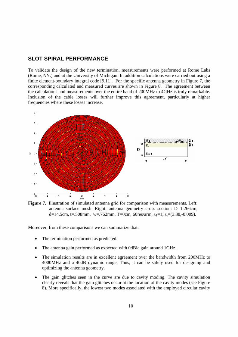
SLOT SPIRAL PERFORMANCE To validate the design of the new termination, measurements were performed at Rome Labs (Rome, NY.) and at the University of Michigan. In addition calculations were carried out using a finite element-boundary integral code [9,11]. For the specific antenna geometry in Figure 7, the corresponding calculated and measured curves are shown in Figure 8. The agreement between the calculations and measurements over the entire band of 200MHz to 4GHz is truly remarkable. Inclusion of the cable losses will further improve this agreement, particularly at higher frequencies where these losses increase.
Figure 7. Illustration of simulated antenna grid for comparison with measurements. Left: antenna surface mesh. Right: antenna geometry cross section: D=1.266cm, d=14.5cm, t=.508mm, w=.762mm, T=0cm, 60res/arm, ε1=1; εr=(3.38,-0.009).
Moreover, from these comparisons we can summarize that:
• The termination performed as predicted.
• The antenna gain performed as expected with 0dBic gain around 1GHz.
• The simulation results are in excellent agreement over the bandwidth from 200MHz to 4000MHz and a 40dB dynamic range. Thus, it can be safely used for designing and optimizing the antenna geometry.
• The gain glitches seen in the curve are due to cavity moding. The cavity simulation clearly reveals that the gain glitches occur at the location of the cavity modes (see Figure 8). More specifically, the lowest two modes associated with the employed circular cavity

11
are the TM010 mode at 1.577GHz and the TM110 mode at 2.511GHz. From Figure 8, this is where the antenna’s axial ratio worsens and/or where antenna gain exhibits a glitch. To remove effect of these resonances, we can use a modified cavity shape.
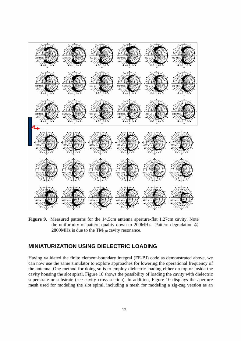
• The axial ratio (a more sensitive parameter) is well predicted by the calculations as well. Except for the three peaks (where moding is likely to occur) the axial ratio is kept below 1.5. Thus, the antenna is circularly polarized over the entire band. This is also verified by the measured patterns given in Figure 9. Shown patterns cover the band from 200MHz to 4000MHz and as seen the axial ratio and broad beamwidth are maintained throughout the band. We remark that these patterns were collected while the transmitting horn antenna was spinning and therefore the pattern oscillations are simply a measure of the axial ratio. Clearly, for broadside radiation the axial ratio (see Figure 8) is quite good, but as expected deteriorates near the horizon (near the plane containing the antenna surface). Since the antenna was actually measured while it was recessed in a circular ground plane, the axial ratio near the horizon is also a measure of the ground plane substructure.
Figure 8. Comparison of full scale simulations and measurements of the broadside gain and axial ratios for the 14.5cm antenna aperture shown in Figure 7.
TM110
TM010
TM110
12
Figure 9. Measured patterns for the 14.5cm antenna aperture-flat 1.27cm cavity. Note
the uniformity of pattern quality down to 200MHz. Pattern degradation @ 2800MHz is due to the TM110 cavity resonance.
MINIATURIZATION USING DIELECTRIC LOADING Having validated the finite element-boundary integral (FE-BI) code as demonstrated above, we can now use the same simulator to explore approaches for lowering the operational frequency of the antenna. One method for doing so is to employ dielectric loading either on top or inside the cavity housing the slot spiral. Figure 10 shows the possibility of loading the cavity with dielectric superstrate or substrate (see cavity cross section). In addition, Figure 10 displays the aperture mesh used for modeling the slot spiral, including a mesh for modeling a zig-zag version as an

136
alternative configuration. The later is a possible printing of the slot aimed at improving bandwidth.
d
εs
d
Figure 10. Geometry of considered archimedean spiral antennas.
Name Diel.
const. tan(δ) Thickness (cm)
RT/Duroid 5880 (ε1) 2.2 0.0009 0.0508, 0.08, 0.127, 0.254, 0.508 RO4003 (ε2) 3.38 0.0027 0.0508, 0.08, 0.127, 0.254, 0.508 RO3006 (ε3) 6.15 0.0025 0.0508, 0.08, 0.127, 0.254, 0.508 RO3010 (ε4) 10.2 0.0035 0.0508, 0.08, 0.127, 0.254, 0.508
Table 1. Parameters of the substrates employed in the present analysis. To assess the miniaturization afforded by the various re-design approaches, we need to establish some mathematical means for doing so. For narrowband antennas, miniaturization is measured by the shift in the resonant frequency. For broadband traveling wave spiral antenna operating in the first mode, an appropriate measure of miniaturization is to find the ratio of the physical antenna diameters, for which antennas have been determined to deliver the same relative gain. For our case, a way for evaluating antenna miniaturization is to measure the magnetic current propagation constant (i.e. the electrical length) along the spiral arms. Since the electrical length of the spiral slot arms will vary depending on the dielectric loading, the ratio of the electric lengths for the loaded and unloaded spiral will give a miniaturization estimate. This is an appropriate approach for the straight and isolated transmission line. However, radiation losses, proximity coupling between spiral arms, reflections inside the cavity, and the inherent non-TEM nature of the slot line will cause distortions in both amplitude and phase of the propagating magnetic current. The total electric fields inside the spiral arms with clear “shrinking” of radiation regions when dielectric constant increases are shown in Figure 11, and the magnetic current phase progression for the same dielectrics is given in Figure 12. As expected, increased dielectric constant leads to longer line, and consequently higher miniaturization factor.

14
Figure 11. Total electric field over the spiral slot for various substrates, at f=2.2GHz.
Free space slot spiral
Figure 12. Magnetic current propagating in the spiral slot for various dielectric constants. To determine the miniaturization factor based on the electrical length of the spiral arms, we can use a transmission line (TL) model approach or the spiral mode approach [9]. Based on the TL model, we would unwrap the spiral arms and compute the electrical lengths for various loadings (θunloaded, θloaded) to yield the miniaturization factor

15
unloaded
loadedTLMF
θθ
=
(1).
As shown in [9] the miniaturization factor for the spiral mode model is the square root of MFTL and it is used in further computations:
TLunloaded
loadedSM MFMF ==
θθ
(2).
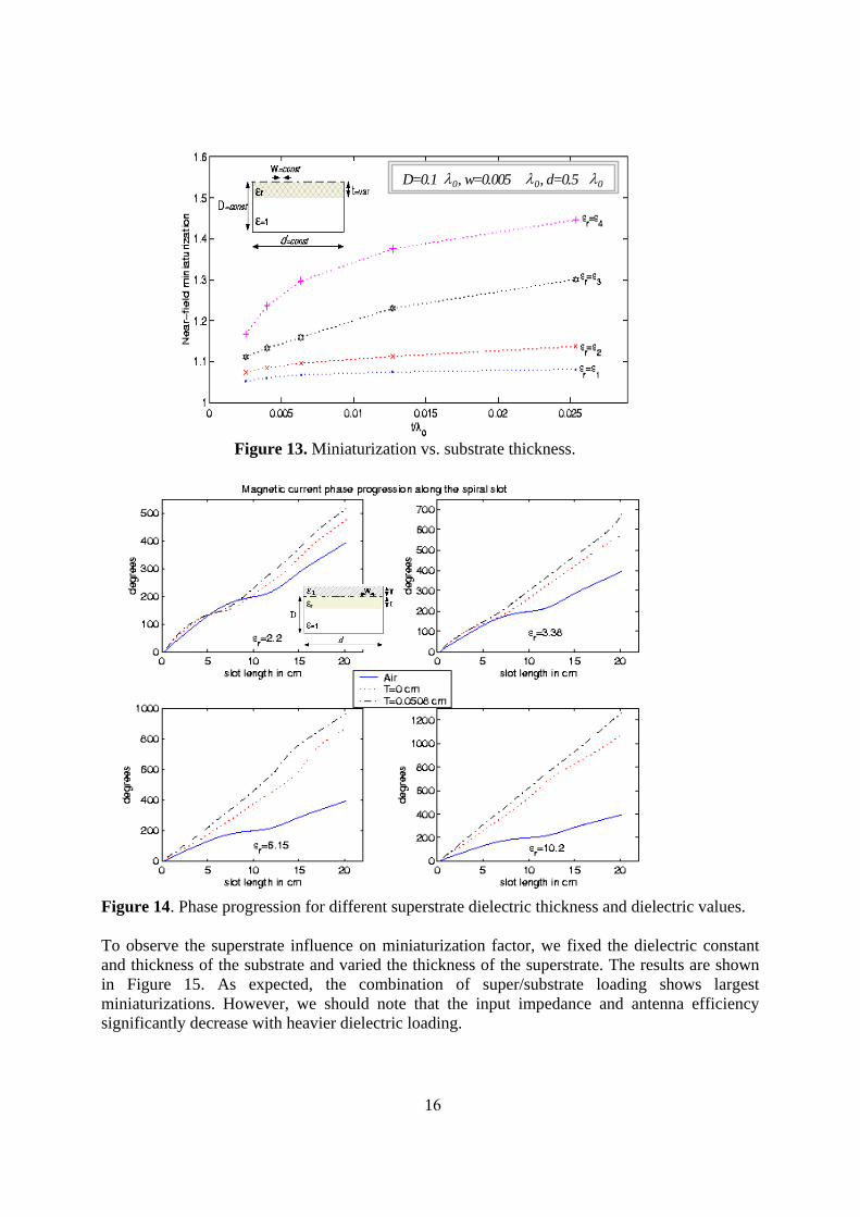
Depending on the spiral growth ratio and the number of turns used to construct the antenna, MF will translate to some physical miniaturization factor. With this in mind, we next proceed to examine the miniaturization amount as the various parameters of the slot spiral and associated cavity are changed. In all cases an archimedean spiral having a diameter d=10cm was used with a growth ratio of a=0.3cm/rad, and dielectrics from the standard choices given in Table 1. Also, the spiral was terminated with lossy Klopfenstain taper[14], using 41 resistors/arm with values varying from 2383Ω to 163Ω as discussed earlier. Below we consider the miniaturization for various substrate/superstrate parameters. MF=MF(t); t - substrate thickness on miniaturization: Figure 13 shows the miniaturization factor (2) as function of the substrate thickness for dielectrics listed in Table 1. The curves in Figure 1 confirm our expectation that thicker substrates, lead to higher miniaturization factors and that the higher dielectric constants lead to same effects. MF=MF(T); T- superstrate effect on miniaturization: It is well known that the introduction of a superstrate (along with substrate) can further improve miniaturization. The phase progression for different substrates is shown in Figure 14. The solid line (blue) represents the unloaded spiral antenna [superstrate (ε1=1) and substrate (εr=1)]. After introducing the dielectric loading inside the cavity (just below the spiral slot plane), we clearly observe an increase in the electrical length of the slot (red dot line). Introduction of an additional superstrate dielectric loading (with the ε1=εr) further increases the electrical length of the antenna (black dot-dash line). From this data, the appropriate near-field miniaturization factors can be easily obtained. We can also observe coupling effects between the spiral arms, as well as coupling due to reflections from the cavity. The observed non-linear phase progressions are due to these couplings as well as radiation losses.
16
D=0.1 λ0, w=0.005 λ0, d=0.5 λ0
Figure 13. Miniaturization vs. substrate thickness.
Figure 14. Phase progression for different superstrate dielectric thickness and dielectric values. To observe the superstrate influence on miniaturization factor, we fixed the dielectric constant and thickness of the substrate and varied the thickness of the superstrate. The results are shown in Figure 15. As expected, the combination of super/substrate loading shows largest miniaturizations. However, we should note that the input impedance and antenna efficiency significantly decrease with heavier dielectric loading.

17
sD=0.044λ0, t=0.0186λ0, w=0.0073λ0,,
d=0.733λ0, εr=ε2
Figure 15. Miniaturization vs. superstrate thickness.
SIX-INCH APERTURE DEVELOPMENT To experimentally determine the antenna properties vs. various spiral parameters, we designed and fabricated a number of slot spiral antennas. Here we present six 6” articles (actual distance between spiral arm ends is ~5.475”) built on 62.5mils thick FR-4. They were thoroughly studied, and some conclusions will be presented in this report. First, we start with the basic Archimedean spiral (a=0.2817cm/rad) shown in Figure 15. Measured results are compared with the initial design of an unloaded slot spiral antenna residing on a shallow, 250mills deep cavity. We observe significant far field miniaturization mainly due to the dielectric loading and deeper cavity (D=1”). The miniaturization factor of 1.32 was observed at the low frequency operation.
+
A1A1
D=2.54cm, d=14.57cm, t=.157cm,30res/arm, w=.0762cm, εs-=(4.25,-.0595), a=.2817cm/rad.
d
t
D
wεs
d
t
D
wεs
4325.228.331.831.7FFMF [%]
1.16.884.668.506.404fA1 [GHz]
2.051.182.932.742.592fID [GHz]
50-5-10-15G [dBic]
4325.228.331.831.7FFMF [%]
1.16.884.668.506.404fA1 [GHz]
2.051.182.932.742.592fID [GHz]
50-5-10-15G [dBic]
Figure 16. Basic 6” antenna A1: geometry and comparison with the initial design.
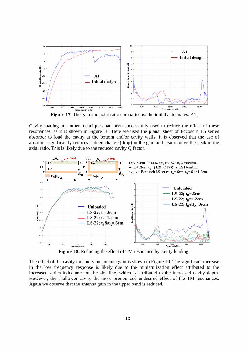
Appropriate CP gain and broadside axial ratio comparisons are given in Figure 17. The existence of the TM110 mode was clearly noticeable, thus resulting in the gain drop and AR peak at approximately 2.65GHz. Reduction of the cavity thickness can control the impact of the resonance. However, the drawback is that the gain will be significantly decreased at the higher band.
18
A1Initial design
A1Initial design
A1Initial design
A1Initial design
Figure 17. The gain and axial ratio comparisons: the initial antenna vs. A1.
Cavity loading and other techniques had been successfully used to reduce the effect of these resonances, as it is shown in Figure 18. Here we used the planar sheet of Eccosorb LS series absorber to load the cavity at the bottom and/or cavity walls. It is observed that the use of absorber significantly reduces sudden change (drop) in the gain and also remove the peak in the axial ratio. This is likely due to the reduced cavity Q factor.
D=2.54cm, d=14.57cm, t=.157cm, 30res/arm, w=.0762cm, εs-=(4.25,-.0595), a=.2817cm/radεA,µA – Eccosorb LS series, tA=.6cm, tB=.6 or 1.2cm. tB tB
UnloadedLS-22; tB=.6cmLS-22; tB=1.2cmLS-22; tB&tA=.6cm
UnloadedLS-22; tB=.6cmLS-22; tB=1.2cmLS-22; tB&tA=.6cm
D=2.54cm, d=14.57cm, t=.157cm, 30res/arm, w=.0762cm, εs-=(4.25,-.0595), a=.2817cm/radεA,µA – Eccosorb LS series, tA=.6cm, tB=.6 or 1.2cm. tBtB tBtB
UnloadedLS-22; tB=.6cmLS-22; tB=1.2cmLS-22; tB&tA=.6cm
UnloadedLS-22; tB=.6cmLS-22; tB=1.2cmLS-22; tB&tA=.6cm
Figure 18. Reducing the effect of TM resonance by cavity loading.
The effect of the cavity thickness on antenna gain is shown in Figure 19. The significant increase in the low frequency response is likely due to the miniaturization effect attributed to the increased series inductance of the slot line, which is attributed to the increased cavity depth. However, the shallower cavity the more pronounced undesired effect of the TM resonances. Again we observe that the antenna gain in the upper band is reduced.
19
Figure 19. Antenna gain vs. cavity thickness.
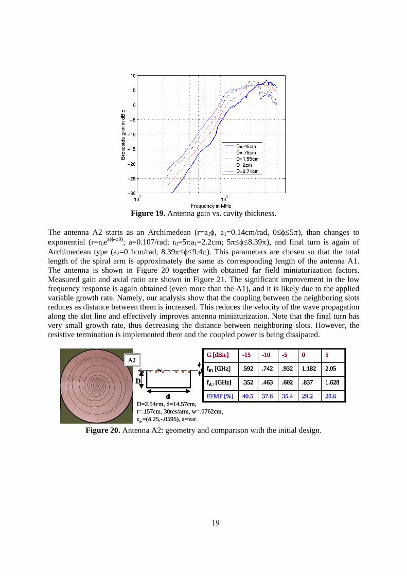
The antenna A2 starts as an Archimedean (r=a1φ, a1=0.14cm/rad, 0≤φ≤5π), than changes to exponential (r=r0ea(φ-φ0); a=0.107/rad; r0=5πa1=2.2cm; 5π≤φ≤8.39π), and final turn is again of Archimedean type (a2=0.1cm/rad, 8.39π≤φ≤9.4π). This parameters are chosen so that the total length of the spiral arm is approximately the same as corresponding length of the antenna A1. The antenna is shown in Figure 20 together with obtained far field miniaturization factors. Measured gain and axial ratio are shown in Figure 21. The significant improvement in the low frequency response is again obtained (even more than the A1), and it is likely due to the applied variable growth rate. Namely, our analysis show that the coupling between the neighboring slots reduces as distance between them is increased. This reduces the velocity of the wave propagation along the slot line and effectively improves antenna miniaturization. Note that the final turn has very small growth rate, thus decreasing the distance between neighboring slots. However, the resistive termination is implemented there and the coupled power is being dissipated.
A2A2
D=2.54cm, d=14.57cm, t=.157cm, 30res/arm, w=.0762cm, εs-=(4.25,-.0595), a=var.
d
tD
wεs
d
tD
wεs
20.629.235.437.640.5FFMF [%]
1.628.837.602.463.352fA1 [GHz]
2.051.182.932.742.592fID [GHz]
50-5-10-15G [dBic]
20.629.235.437.640.5FFMF [%]
1.628.837.602.463.352fA1 [GHz]
2.051.182.932.742.592fID [GHz]
50-5-10-15G [dBic]
2
Figure 20. Antenna A2: geometry and comparison with the initial design.

20
A2Initial design
A2Initial design
A2Initial design
A2Initial design
A2Initial design
A2Initial designA2Initial design
Figure 21. The gain and axial ratio comparisons: the initial antenna vs. A2.
The Archimedean spiral antenna A3 is also designed to have approximately the same arm length as antenna A1. Spiral growth utilizes four different growth rates:
• a1=0.2cm/rad, 0≤φ≤3π; • a2=0.2817cm/rad, 3π≤φ≤5.78π; • a3=0.85cm/rad, 5.78π≤φ≤6.85π; • a4=0.12cm/rad, 6.85π≤φ≤8π.
The antenna is shown in Figure 22, while corresponding gain and axial ratio characteristics are given in Figure 23. Again we observe that the larger distance between neighboring slots at the outside of the spiral improves the low frequency response. Miniaturization factors up to 42% have been obtained.
A3A3
D=2.54cm, d=14.57cm, t=.157cm,30res/arm, w=.0762cm, εs-=(4.25,-.0595), a=var.
d
tD
wεs
d
tD
wεs
33.227.535.338.341.5FFMF [%]
1.369.857.603.458.346fA1 [GHz]
2.051.182.932.742.592fID [GHz]
50-5-10-15G [dBic]
33.227.535.338.341.5FFMF [%]
1.369.857.603.458.346fA1 [GHz]
2.051.182.932.742.592fID [GHz]
50-5-10-15G [dBic]
3
Figure 22. Antenna A3: geometry and comparison with the initial design.
A3Initial designA3Initial design
A3Initial designA3Initial design
Figure 23. The gain and axial ratio comparisons: the initial antenna vs. A3.

214
The antenna A4 is an exponential antenna with modified last turn to a small growth rate Archimedean. The arm length is approximately the same as antenna A1 (10% smaller). The antenna growth is described as follows: (a=0.15/rad, r0=2.84mm, 0≤φ≤6.635π); (aarch=0.16cm/rad, 6.635π≤φ≤8.1π). This modification again allows for better use of given surface area with radiating slot. Also, by having resistive termination as far as possible from the antenna center the power dissipation is more effective, and aperture efficiency is better at the low band. Its geometry is shown in Figure 24, and measured gain and axial ratio are given in Figure 25. This configuration shows 41% far-field miniaturization.
Figure 24. Antenna A4: geometry and comparison with the initial design.
A4Initial design
A4Initial design
A4Initial designA4Initial designA4Initial design
A4Initial designA4Initial design
Figure 25. The gain and axial ratio comparisons: the initial antenna vs. A4.
The meanderline concept is known to reduce the effective velocity of the propagating wave. Here, we implement the meanderline slotline within the basic spiral geometry A3. The geometry is shown in Figure 26, and measured gain and axial ratio are given in Figure 27. We observe a significant improvement in the far field miniaturization factor at the low frequencies. The gain drop at 600MHz is likely attributed to the uneven meanderline growth so that the propagating wave goes through in and out phase thus constructively and destructively adding in the far field as frequency is swept. Also, the lower section of the meanderline is closer to the neighboring slot (enhance the coupling) so that the gain is decreased as compared to the case when this distance would increase with the spiral growth. Because of this, the axial ratio is little higher with many ripples in the band. The magnitude of the gain ripple can be controlled by the applied resistive taper, as is shown in the Figure 28. As expected longer resistive termination reduce the amplitude of the gain change, but also the overall gain at lower band is decreased.
A4A4
D=2.54cm, d=14.57cm, t=.157cm,30res/arm, w=.0762cm, εs-=(4.25,-.0595), a=var.
d
t
D
wεs
d
t
D
wεs
8.329.736.339.441FFMF [%]
1.88.831.594.450.349fA1 [GHz]
2.051.182.932.742.592fID [GHz]
50-5-10-15G [dBic]
8.329.736.339.441FFMF [%]
1.88.831.594.450.349fA1 [GHz]
2.051.182.932.742.592fID [GHz]
50-5-10-15G [dBic]
4

22
A5A5
D=2.54cm, d=14.57cm, t=.157cm,30res/arm, w=.0762cm, εs-=(4.25,-.0595), a=var.
d
tD
wεs
d
tD
wεs
28.514.153.453.756.7FFMF [%]
1.4651.015.434.343.256fA1 [GHz]
2.051.182.932.742.592fID [GHz]
50-5-10-15G [dBic]
28.514.153.453.756.7FFMF [%]
1.4651.015.434.343.256fA1 [GHz]
2.051.182.932.742.592fID [GHz]
50-5-10-15G [dBic]
5
Figure 26. Meanderline antenna A5: geometry and comparison with the initial design.
A5Initial designA5Initial designA5Initial design
A5Initial designA5Initial designA5Initial design
Figure 27. The gain and axial ratio comparisons: the initial antenna vs. A5.
30 resistors (regular)14 resistors (short)30 resistors (long)
30 resistors (regular)14 resistors (short)30 resistors (long)
.252.130 res. (long)
3.28.514 res. (short)
.354.130 res. (regular)
∆@ ∆.9GHz in dB
∆ @.45GHz in dB
.252.130 res. (long)
3.28.514 res. (short)
.354.130 res. (regular)
∆@ ∆.9GHz in dB
∆ @.45GHz in dB
Figure 28. The gain variations for various resistive tapers.
Finally, antenna A6 is similar to the meanderline antenna A5. The only difference is in the shape of the meanderline sections. The spiral growth is also based on antenna A3. The geometry is shown in Figure 29 and gain and axial ratio measured results are given in Figure 30. Far field miniaturization factors of up to 57% are observed.

23
A6A6
D=2.54cm, d=14.57cm, t=.157cm, 30res/arm, w=.0762cm, εs-=(4.25,-.0595), a=var.
d
tD
wεs
d
tD
wεs
28.514.555.754.456.9FFMF [%]
1.4651.011.413.338.255fA1 [GHz]
2.051.182.932.742.592fID [GHz]
50-5-10-15G [dBic]
28.514.555.754.456.9FFMF [%]
1.4651.011.413.338.255fA1 [GHz]
2.051.182.932.742.592fID [GHz]
50-5-10-15G [dBic]
6
Figure 29. Meanderline antenna A6: geometry and comparison with the initial design.
A6Initial designA6Initial designA6Initial design
A6Initial designA6Initial designA6Initial design
Figure 30. The gain and axial ratio comparisons: the initial antenna vs. A6.
HF/VHF to L-BAND DESIGN To develop an antenna that operates from VHF to L-band we increased the aperture size to 18”, and designed and fabricated the antennas shown in Figure 31. A7 has constant, very large growth rate (a=0.8038cm/rad) whereas A8 has variable growth rate and is loaded with a carefully designed meanderline. The common geometrical parameters for these antennas are: [D,d,t,w,ε, #res/arm] = [6.1cm,45.2cm,3.175mm,.762mm,4.15,40].
D
d
LS-22
tw ε
LS-30
A7 A8
D
d
LS-22
tw ε
LS-30
A7A7 A8A8
Figure 31. Geometry of 18” antennas A7 and A8.

24
The low and mid band frequency measurements (up to 1500MHz) were conducted at Rome, NY (Figure 32 shows a picture of the antenna in a large 12.2m×12.2m ground plane). Measured gains for both antennas are compared with the scaled versions of A1 and A6, and the comparisons are shown in Figure 33. We observe significant improvement in the performance of the meanderline antenna A8 (7dB higher gain than Ant4 at 100MHz). Also, due to the variable growth rate of the meanderline antenna (smaller a toward the center of the aperture), the gain of A8 is significantly higher in the upper band as compared to the gain of A7 (5dB at 2GHz).
Figure 32. Outdoor measurement site at Rome, NY.
A7A8A1scA6sc
A7A8A1scA6sc
A7A8A1scA6sc
Figure 33. Broadside gain of 18” antennas.
The detrimental effects of numerous TM1x waveguide modes on the axial ratio are depicted in Figure 34 where the empty cavity configuration is compared to the corresponding absorber
258
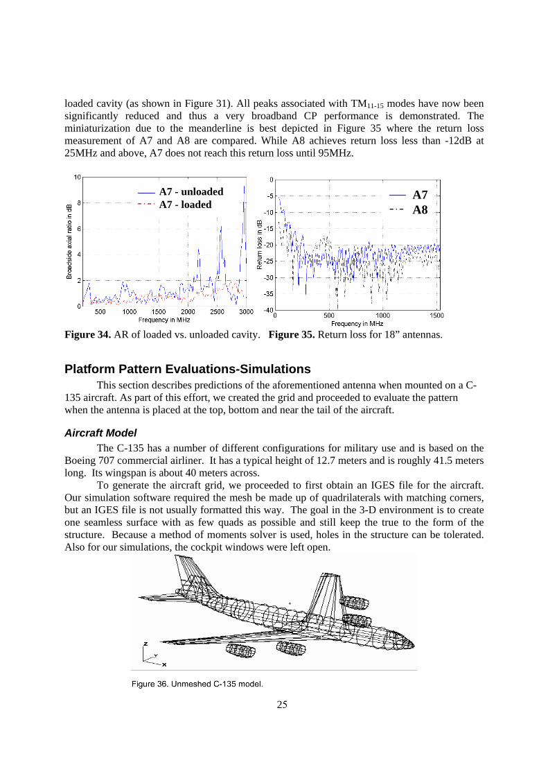
loaded cavity (as shown in Figure 31). All peaks associated with TM11-15 modes have now been significantly reduced and thus a very broadband CP performance is demonstrated. The miniaturization due to the meanderline is best depicted in Figure 35 where the return loss measurement of A7 and A8 are compared. While A8 achieves return loss less than -12dB at 25MHz and above, A7 does not reach this return loss until 95MHz.
A7 - unloadedA7 - loadedA7 - unloadedA7 - loadedA7 - unloadedA7 - loaded
A7A8A7A8A7A8
Figure 34. AR of loaded vs. unloaded cavity. Figure 35. Return loss for 18” antennas.
Platform Pattern Evaluations-Simulations This section describes predictions of the aforementioned antenna when mounted on a C-135 aircraft. As part of this effort, we created the grid and proceeded to evaluate the pattern when the antenna is placed at the top, bottom and near the tail of the aircraft.
Aircraft Model The C-135 has a number of different configurations for military use and is based on the Boeing 707 commercial airliner. It has a typical height of 12.7 meters and is roughly 41.5 meters long. Its wingspan is about 40 meters across. To generate the aircraft grid, we proceeded to first obtain an IGES file for the aircraft. Our simulation software required the mesh be made up of quadrilaterals with matching corners, but an IGES file is not usually formatted this way. The goal in the 3-D environment is to create one seamless surface with as few quads as possible and still keep the true to the form of the structure. Because a method of moments solver is used, holes in the structure can be tolerated. Also for our simulations, the cockpit windows were left open.
269
Due to difficulty in meshing, the wingtips and tail tips were also left open. Unless antennas are placed directly on these locations, these holes should not have any effect. Also, for simplification the engines were modeled as open cylindrical shells of the same shape. Attempts were made to reduce the risk of long and thin quads, and ensure that relatively small quads would not be necessary. Once the whole structure was simplified in this way, the IGES file looked like the one in Figure 36.
The fuselage of the model is 4.1 meters tall and 3.7 meters wide along much of the length. The modeled wingspan is 38.7 meters and the tail span is 12.6 meters. Also, the overall length of the aircraft model is 40 meters. These dimensions are all near that of the actually C-135 dimensions stated above. Using MSC Patran’s built-in meshing capabilities, a mesh of quadrilaterals was created. Each quad was defined by nine nodes, one at each corner, at the center of each side, and at the center of the quad itself. To make the model easier for checking errors in the mesh, the entire aircraft was split into three sections: cockpit, wings and midsection, and tail section.
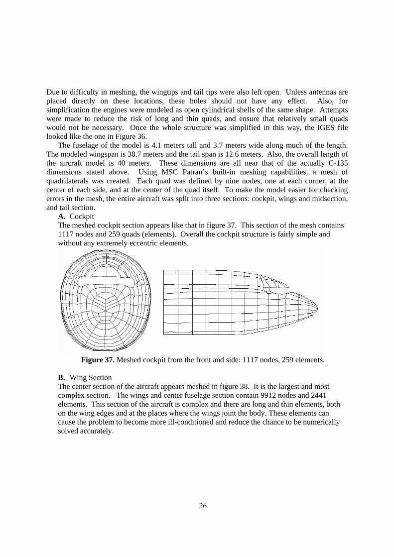
A. Cockpit The meshed cockpit section appears like that in figure 37. This section of the mesh contains 1117 nodes and 259 quads (elements). Overall the cockpit structure is fairly simple and without any extremely eccentric elements.
Figure 37. Meshed cockpit from the front and side: 1117 nodes, 259 elements.
B. Wing Section The center section of the aircraft appears meshed in figure 38. It is the largest and most complex section. The wings and center fuselage section contain 9912 nodes and 2441 elements. This section of the aircraft is complex and there are long and thin elements, both on the wing edges and at the places where the wings joint the body. These elements can cause the problem to become more ill-conditioned and reduce the chance to be numerically solved accurately.

27
Figure 38. Meshed wing section: 9912 nodes, 2441 elements.
C. Tail Section The tail section is shown meshed in figure 39. It contains 2485 nodes and 617 elements. Like the wing section, it is a very complex structure. Because of how the tail pieces fit to the plain, especially the fin, some problem elements may be created.
Figure 39. Meshed tail section: 2485 nodes, 617 elements.
A mesh of the whole aircraft can be seen in figure 40. It has a total of 13515 nodes with
3317 elements.

28
Figure 40. Entire C-135 meshed: 13515 nodes, 3317 elements.
Platform Analysis Radiation patterns were taken with antennas placed at three different locations on the aircraft, and at two frequencies. An antenna was placed on the top of the plane between the wings, then underneath between the wings, and finally in front of the tail, on the top. Figures 41-43 show the three antenna locations. Tests were made and data taken for both 30 and 50 MHz frequencies.
Figure 41. Antenna above center. Figure 42. Antenna below center.
Figure 43. Antenna above plane and in front of tail.
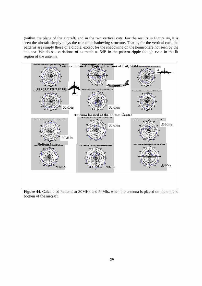
For simulations, the slot-spiral was represented by a pair of crossed-magnetic dipoles placed one eighth of a wavelength away from the surface. Pattern cuts were then obtained in the horizontal
29
(within the plane of the aircraft) and in the two vertical cuts. For the results in Figure 44, it is seen the aircraft simply plays the role of a shadowing structure. That is, for the vertical cuts, the patterns are simply those of a dipole, except for the shadowing on the hemisphere not seen by the antenna. We do see variations of as much as 5dB in the pattern ripple though even in the lit region of the antenna.
Figure 44. Calculated Patterns at 30MHz and 50Mhz when the antenna is placed on the top and bottom of the aircraft.

303
FLIGHT TEST DATA As given in Appendix A, in-flight measured data were conducted by AFRL. Such flight data were collected by mounting the antenna at the bottom of the C135E serial No. 600372 (see Figure 45). The tests were conducted at 50.5MHz, 144.05MHz, 432.05MHz, 902.05MHz and 1296.05MHz at a power level of about 10Watts at each frequency. We remark that the cavity-backed slot spiral placed at the bottom of the aircraft was covered with a radome whereas the isolated antenna tests at Rome Labs (see figure 33) did not include any radome effects. It would have been appropriate to account for such radome effects for proper data comparison. However, no specific information on the radome materials are available to allow for such an evaluation. Therefore only a qualitative comparison will be given. Indeed, the AFRL measurements do verify that the peak gain is at about 600MHz and above, whereas at 50MHz the measured signal is 20dB below the peak. Our isolated antenna measurements and calculations at 600MHz (see Figure 33) show a gain of +5 to +7dBic which reduces to -25dBic at 50MHz. Thus, both in-situ and stand-alone measurements and calculations display the same gain roll-off.

31
Figure 45. Sketch of the C135E serial No. 600372 and a photo of the antenna (with radome at the right) mounting at the aircraft bottom.

32
CONCLUSION This report presented a summary of the design procedure that ultimately led to a very broadband (VHF/UHF to L-band), circularly polarized thin cavity backed spiral slot antenna. This was achieved using a new meanderline concept to improve the low frequency response, together with variable growth rate to improve the high frequency response. Excellent return loss, axial ratio and gain performances are documented from 50MHz and above. Measurements were conducted for the 18” antenna aperture at the Rome Labs outdoor facility and these verify the analysis. Also, in-fight data on a C135 aircraft provided for additional qualitative verification.

33
REFERENCES 1. R. Bawer, J. J. Wolfe, “A Printed Circuit Balun for Use with Spiral Antennas,” IRE Trans.
Microwave Theory Tech., Vol. MTT-8, pp. 319--325, May, 1960. 2. R. G. Corzine and J. A. Mosko, Four-Arm Spiral Antennas, Artech House, 1990. 3. M. W. Nurnberger, J. L. Volakis, “Slot Spiral Antenna with Integrated Balun and Feed,”
U.S. Patent No. 5,815,122, issued 29 September 1998. 4. M. W. Nurnberger, J. L. Volakis, “A New Planar Feed for Slot Spiral Antennas,” IEEE
Trans. Antennas Propagat., Vol. AP-44, No. 1, pp. 130-131, January 1996. 5. M. W. Nurnberger, J. L. Volakis, D.T. Fralick, F.B. Beck, “A Planar Slot Spiral for
Conformal Vehicle Applications,” 18th Meeting and Symposium of Antenna Measurement Techniques Association, Seattle, WA, Sept. 1996.
6. M.W. Nurnberger and J.L. Volakis, “A planar slot spiral for mobile communications,” 19th American Measurement Techniques Assoc. (AMTA), Symposium Digest , pp. 61-67, Boston, MA, 1997.
7. M. Nurnberger, J. Volakis and T. Ozdemir, “A Planar Slot Spiral for Multifunction Communication Apertures,” 1998 IEEE Antennas and Propagat Symposium, Atlanta, GA, pp. 774-777.
8. M. W. Nurnberger, M. Abdel-Moneum, J. L. Volakis, “New Techniques for Extremely Broadband Planar Slot Spiral Antennas,” 1999 AP-S International Symposium and URSI Radio Science Meeting, Orlando, FL, July 1999.
9. D. S. Filipovic, M. W. Nurnberger, J. L. Volakis, “Ultra wide-band slot spiral with dielectric loading: measurements and simulations”, 2000 AP-S International Symposium and URSI Radio Science Meeting, Salt Lake City, UT, July 2000.
10. J. D. Dyson, ”The Equiangular Spiral Antenna,” IRE Trans. Antennas Propagat., Vol. AP-7, pp. 181-187, April, 1959.
11. T. Ozdemir, J.L. Volakis and M.W. Nurnberger, “Analysis of Thin Multioctave Cavity-backed Slot Spiral Antennas,” IEE Proceedings-Microwave, Antennas and Propagation, Vol.146, pp. 447-454, December 1999.
12. M. Turner, “Spiral Slot Antenna,” U.S. patent 2,863,145, December 1958. 13. M.W. Nurnberger and J.L. Volakis, “Extremely broadband slot spiral antennas with shallow
reflecting cavities,” Electromagnetics, Vol 20, No. 4, pp. 357-376. 14. R. W. Klopfenstein, “A Transmission Line Taper of Improved Design,” Proc. IRE, Vol. 44,
pp. 31--35, January, 1956.

347
APPENDIX A: Blurb from the AFRL Web Site-May 2004 Accomplishments
http://www.afrl.af.mil/accomprpt/may04/accompmay04.htm
Volakis Spiral Antenna Flight Test Successful
The Information Directorate performed a successful flight test of the Volakis spiral antenna. The directorate acquired a data set containing signal strength and position information during five passes over Wright-Patterson Air Force Base at approximately 26,000 ft. The radome and antenna assembly were mechanically stable at air speeds ranging from 300 to 450 knots indicated air speed.
Post-flight inspection of the assembly showed no flight-related damages. The antenna successfully acquired signals on five distinct frequencies from 50 MHz up to 1.24 GHz. The test data sets are presently being correlated with position and attitude data from the aircraft’s inertial navigation system. (Ms. H. Demers, AFRL/IFGD, (937) 255-4947 x3405 and Mr. R. French, AFRL/IFGD (contractor), (937) 255-4947, x3418)

35
Appendix B: Slot Spiral Antenna Flight Test Report by Robert French
Robert French RF Instrumentation Engineer
AFRL/IFGD WPAFB, Dayton, Ohio
Background The Rome Research Station (RRS) has developed a technique for measuring the effects of airframes and external stores on antenna radiation pattern characteristics of antenna systems in a simulated flight environment. Measurements of this type have been performed in the past at the AFRL Newport Research Facility, with various antennas on full size airframes. The data obtained is used to optimize the antenna radiation characteristics without the requirement for an extensive flight test program. Objective The objective of flight testing the University of Michigan Slot Spiral (MSS) antenna is to provide comparative performance data collected under actual flight conditions. Test Philosophy A test sequence was devised to produce performance data that will allow comparison with that produced by RRS. This will allow RRS to assess the accuracy of the computer algorithms used for predicting antenna pattern performance in the presence of airframes and external stores in flight. Because of the high cost of flight hours, tests have been designed to combine ground testing with airborne tests wherever possible. Test Description A verification flight test of the MSS antenna is proposed, using the lower forward Radome to contain the structure. The Test Goal is to produce multi-frequency pattern response data that contains received signal strength, and aircraft altitude, position, and attitude information. The test will require a ground based signal source, and an aircraft based spectrum analyzer and data collection system. The ground based transmitter will emit a five seconds on, one second off CW signal on or about 50.05, 144.05, 432.05, 902.05, 1296.05 MHz, at a power level of about 10 W on each frequency. The on/off pattern will help to clearly identify the correct signal if it becomes buried in ground based interference. The spectrum analyzer will receive that signal and transfer signal level data to the data recorder along with aircraft inertial navigation system (INS) and global positioning system (GPS) data. The INS/GPS data will record aircraft attitude, altitude and position data. Data will be recorded at about one data point per second.
36 39
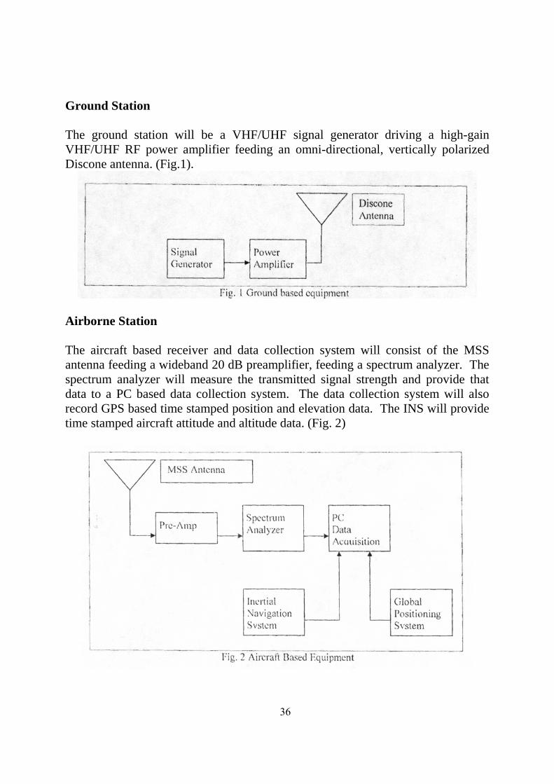
Ground Station The ground station will be a VHF/UHF signal generator driving a high-gain VHF/UHF RF power amplifier feeding an omni-directional, vertically polarized Discone antenna. (Fig.1).
Airborne Station The aircraft based receiver and data collection system will consist of the MSS antenna feeding a wideband 20 dB preamplifier, feeding a spectrum analyzer. The spectrum analyzer will measure the transmitted signal strength and provide that data to a PC based data collection system. The data collection system will also record GPS based time stamped position and elevation data. The INS will provide time stamped aircraft attitude and altitude data. (Fig. 2)
37 40
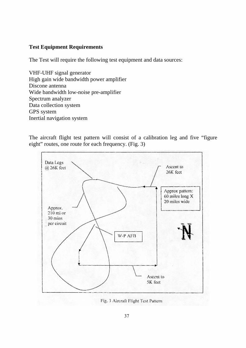
Test Equipment Requirements The Test will require the following test equipment and data sources: VHF-UHF signal generator High gain wide bandwidth power amplifier Discone antenna Wide bandwidth low-noise pre-amplifier Spectrum analyzer Data collection system GPS system Inertial navigation system The aircraft flight test pattern will consist of a calibration leg and five “figure eight” routes, one route for each frequency. (Fig. 3)

38 41
MSS Mod
Proposed Schedule as of Feb 04 Wayne F.
Determine preamp size and power mount?
6 Feb
Wayne, Bob F
Fabricate & Paint metalwork
9-13 Feb
Randy S.
Install low loss coax from under floor 9-13 Feb Maintenance
Fabricate & label RG400 coaxes (between antenna cable-preamp-spectrum analyzer)
1-13 Feb Harvey or Bob F
Install above coax cable in aircraft
17-20 Feb
Install antenna on bracket
17-19 Feb
Randy S., Mike S.
Install antenna & bracket on aircraft (insure good grounding-bracket to aircraft and antenna-burnishing or ground straps)
17-19 Feb
Maintenance, Mike S.
Temp install radome on aircraft (fit check) (leave radome temp installed for Edwards inspection)
18-20 Feb Maintenance, Mike S.
Install coax cables & preamp
17-20 Feb
Mac, Bob F.
EMIC
25 Feb
Allen, Tony
Edwards inspections
2 March
Phil, Wayne
Finalize radome installation for flight
2-3 March
Mint.
Finalize Flight Release
3 March
Phil, Wayne
FCF 4 March/5 March back-up
Note: Aircraft will be out of hanger starting 23 Feb. Assumptions: Antenna fits in radome. No problems installing Radome on aircraft.

39 42
MSS Antenna Flight Ground Station Test Procedure
Robert French RF Instrumentation Engineer
All steps in this procedure must be logged, time stamped, and initialed as they are completed. All test equipment should be energized for a reasonable amount of time ahead of flight time in order to allow the equipment to thermally stabilize. External antenna switch should be set to select the rooftop coaxial cable. The test technician should not assume that it is properly set, and must physically check it for correct setting at test time. Signal generator should be pre-set to first test frequency, and the function generator set to the correct on-off waveform. A short test transmission should be made to verify by Wattmeter reading that the correct power level is being delivered to the antenna with the correct on and off time intervals. A SATCOM repeater comms check should be made with the aircraft. Approximately ½ hour after take-off, the Flight Test Engineer will contact the Test Technician by SATCOM radio to request the first test signal. The Test Technician will acknowledge that request, establish the test signal, and radio that accomplishment to the Flight Test Engineer. The aircraft will then fly gentle figure 8 patterns which will require approximately ½ hour to complete. At the completion of each figure 8 pattern, the Flight Test Engineer will contact the Test Technician and request that the test equipment be advanced to the next frequency on the list. The Test Technician will repeat the above procedure for each new frequency. When the frequency list is completed, the Flight Test Engineer will contact the Test Technician and request any necessary repeats or declare that the test has been completed. Test Technician will then secure all logs and may disassemble the test set-up if the equipment is immediately required elsewhere. Frequency List; 50.05 MHz, 144.05 MHz, 432.05 MHz, 902.05 MHz, 1.29605 GHz _______________________________________ ____________________ Robert French Date RF Instrumentation Engineer

40
MSS Antenna Flight Ground Station Test Log
Procedure Time Initial Test equipment energized External switch setting verified Signal generator frequency preset Function generator set SATCOM comms check Test Transmission 1st signal energized 2nd signal energized 3rd signal energized 4th signal energized 5th signal energized Repeat Requested? (Y/N) Repeat Completed? (Y/N) Test Completed? (Y/N) Frequency List; 50.05 MHz, 144.05 MHz, 432.05 MHz, 902.05 MHz, 1.29605 GHz _______________________________ _______________________ Test Technician Date

41 44
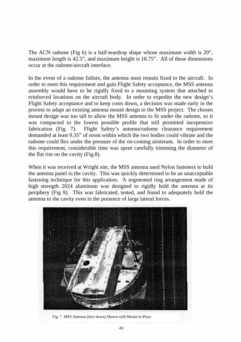
Mounting System and Radome Enclosure An early cost containment proposal was to fit the MSS antenna inside an existing radome that had already been flight qualified. A short study determined that the MSS Antenna could probably be made to fit under a small radome developed under a previous program, the-so-called ACN Radome. It was approximately the correct size, already flight qualified, and immediately available, so it was selected for this project.
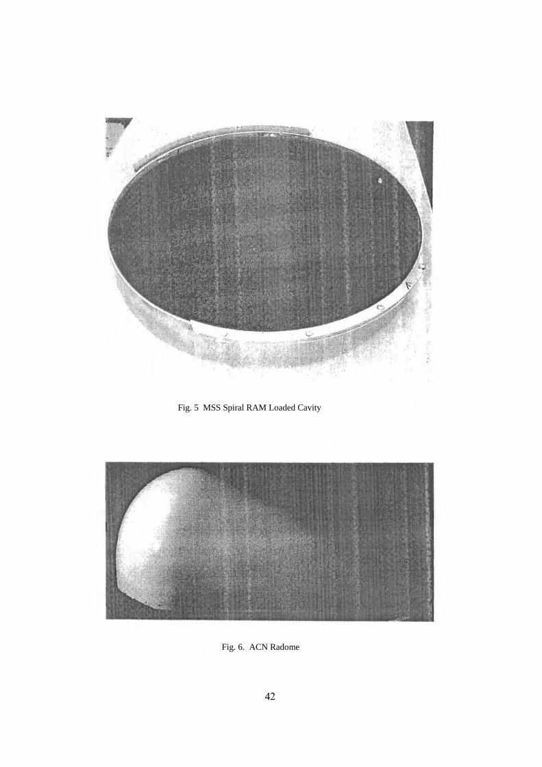
The radiating portion of the MSS antenna is a spiral etched onto printed circuit board material, which was intended to be mounted over a radar absorbing material (RAM) loaded cavity. The antenna radiator (Fig 4) is a flat circular plate whose diameter is about 18 ¼. The RAM loaded cavity (Fig 5), is in the form of a pan about 2 ½” deep, and has a flat run that extends out about another 2”.
42
Fig. 5 MSS Spiral RAM Loaded Cavity
Fig. 6. ACN Radome
46
The ACN radome (Fig 6) is a half-teardrop shape whose maximum width is 20”, maximum length is 42.5”, and maximum height is 18.75”. All of these dimensions occur at the radome/aircraft interface. In the event of a radome failure, the antenna must remain fixed to the aircraft. In order to meet this requirement and gain Flight Safety acceptance, the MSS antenna assembly would have to be rigidly fixed to a mounting system that attached to reinforced locations on the aircraft body. In order to expedite the new design’s Flight Safety acceptance and to keep costs down, a decision was made early in the process to adapt an existing antenna mount design to the MSS project. The chosen mount design was too tall to allow the MSS antenna to fit under the radome, so it was compacted to the lowest possible profile that still permitted inexpensive fabrication (Fig. 7). Flight Safety’s antenna/radome clearance requirement demanded at least 0.35” of room within which the two bodies could vibrate and the radome could flex under the pressure of the on-coming airstream. In order to meet this requirement, considerable time was spent carefully trimming the diameter of the flat rim on the cavity (Fig.8). When it was received at Wright site, the MSS antenna used Nylon fasteners to hold the antenna panel to the cavity. This was quickly determined to be an unacceptable fastening technique for this application. A segmented ring arrangement made of high strength 2024 aluminum was designed to rigidly hold the antenna at its periphery (Fig 9). This was fabricated, tested, and found to adequately hold the antenna to the cavity even in the presence of large lateral forces.
Fig. 7 MSS Antenna (face down) Shown with Mount in-Place 43 4 43
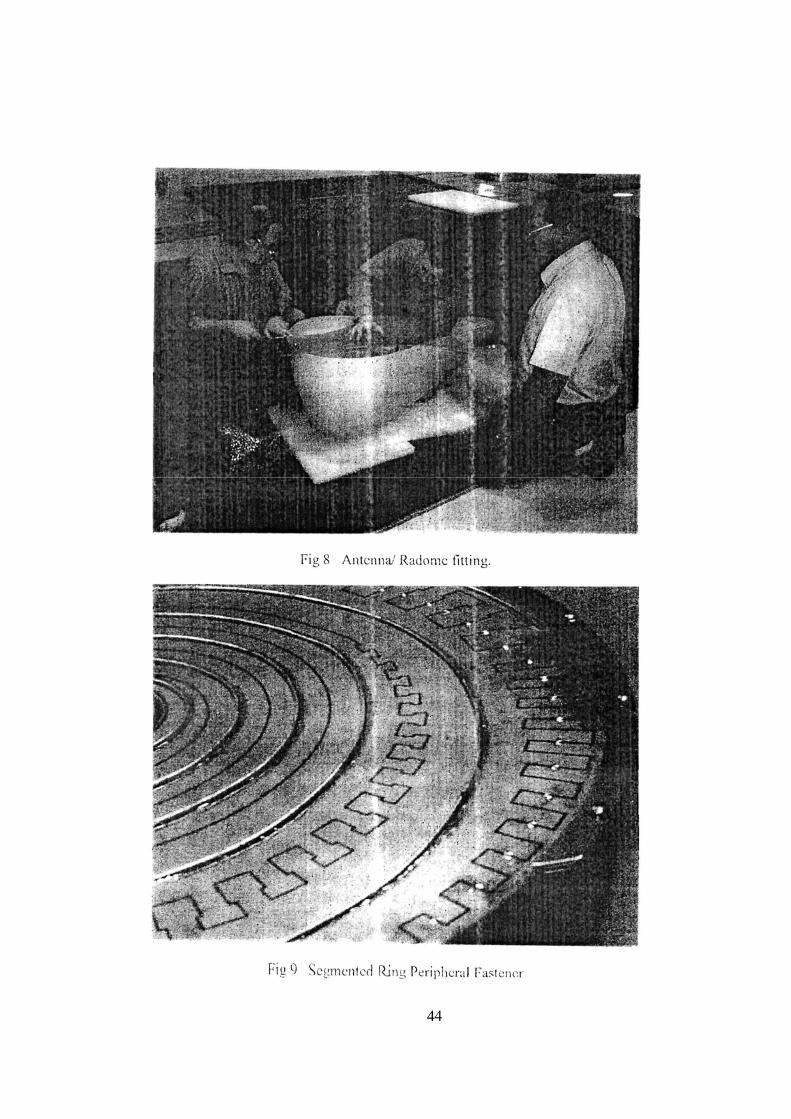
44

4548
RFI/EMC Test Report for MSS Antenna
4 Mar 2004 RFI/EMC Test: On March 2004, a Radio Frequency Interference/Electro-Magnetic Compatibility (RFI/EMC) test was conducted on the MSS Antenna (Figure 10), installation on Aircraft C-135/372. As part of the test, the receive spectrum of the MSS antenna system was recorded (Figure 11), to look for spurious transmissions. No spurious transmissions were found. With the engines running and while on aircraft power, the aircraft’s avionics systems identified in the RFI/EMC Test procedures (Attachment 1) were turned on and the operation checked with all mission equipment turned off. All aircraft systems operated properly. Next, the MSS Antenna system was turned on and it received its normal modulation from the Building 268 ground station. The aircraft’s avionics systems were all rechecked with the antenna radiating. All of the aircraft’s avionics systems continued to operate properly (Attachment 1). Conclusions: The newly installed MSS Antenna system did not cause and RFI/EMC interference with the aircraft’s avionics or safety of flight systems.
CE19/RFI/EMC Test Report2 (Test conducted by A. Johnson and A Sorice, and Certification submitted by A. Johnson.)

46

47
RFI/EMC TEST PROCEDURES FOR VOLAKIS ANTENNA 3 Mar 2004
Objective: Verify that the Radio Frequency Interference/ElectroMagnetic Compatibility (RFI/EMC) generated by the Volakis antenna system receiving in the 50-1500 MHz Band does not interfere with the aircraft’s communications, navigation or safety of flight systems. Test Approach: Turn on the aircraft’s communications, navigation and safety of flight systems and verify they operate properly before the systems under test are turned on. Then turn on the Volakis antenna system. Operate the Volakis antenna system while monitoring the aircraft’s communications, navigation and safety of flight systems. Check for interference to the aircraft systems caused by the Volakis antenna system. Test Procedures: 1. With engines running and on aircraft power, turn on the aircraft’s UHF and VHF radios, TACAN, VOR/II.S/Glide Slope, LNS/GPS, TCAS, IFF, flight systems and radar, and verify they operate properly with the systems under test powered off. 2. Turn on the Volakis antenna system. With the receiver tuned to a VHF frequency of 144.05 MHz receive a VHF CW signal transmitted by the Rooftop Facility. 3. Tune the UHF and VHF radios across the band and check for interference from the Volakis antenna system. 4. Tune the TACAN to the local station and verify it operates properly. 5. Check the VOR/ILS/Glide Slope to see if the Volakis antenna system is causing interference. 6. Check the INS/GPS and verify it operates properly while the Volakis antenna system is in use. 7. Check the TCAS and verify it operates properly while the Volakis antenna system is in use. 8. Check the IFF and verify it operates properly while the Volakis antenna system is in use. 9. Check the flight systems and verify they operate properly while the Volakis antenna system is in use. 10. Check the radar and verify it operates properly while the Volakis antenna system is in use. Operator #1_____________________________________________________________ Operator #2_____________________________________________________________ Results Passed__________________ Failed_________________________

48
Description of Type and Location of External Stores
The Air Force Research Laboratories operates the AFRL C41 Airborne Testbed (ACAT) aircraft model C-135E serial number 600372. This is a highly modified testbed aircraft that can support single or multiple simultaneous experiments, for the purposes of basic research on and practical demonstrations of airborne and satellite based communications and sensor systems. Depending on the mission definitions, the external configuration of the aircraft may be different for every flight. Fig. 13 shows the MSS/Radome installation on the day of the test flight (19MAR04), and ACAT was configured as shown at Figure 12 in the following manner: Device Approximate Frame Station Fuselage Lower Surface from Front to Rear; ACN Radome containing MSS Spiral VHF Blade UHF Turnstile UHF Blade UHF Blade UHF Blade Fuselage Upper Surface from Front to Rear; UHF Blade VHF Blade UHF Hemispherical Primary Experimental Radome UHF Hemispherical UHF Hemispherical Secondary Experimental Radome UHF Turnstile UHF Turnstile UHF Blade UHF Blade
460 640 660 680 980 1150 310 420 430 570 800 860 970 1060 1130 1170 1200 1250
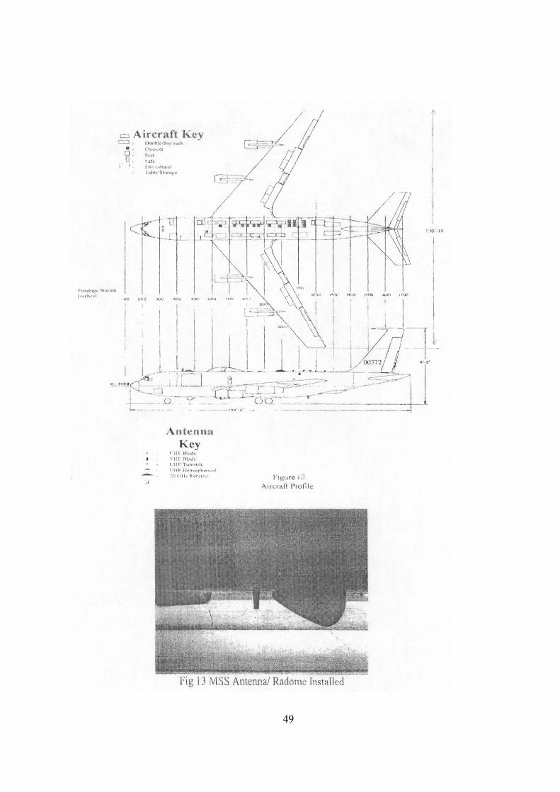
49

50
MSS Antenna Flight Details The flight of the MSS Spiral antenna got off to a rocky start, but initial problems were resolved in time to begin the test. The mission began at take-off at 1032 UTC, and was completed nearly four hours later at 1432 UTC. The MSS Test portion of the mission began at 1050 UTC, and was completed about an hour and a half later at 1223 UTC.
MSS Spiral Antenna Flight Log (ed.)
LOCAL UTC COMMENTS
Arrived hangar 268 Arrived A/C 372 Lt. Duffy arrived A/C 372 Replaced pre-amp battery Pre-amp “on” LED failed Bill Rembacz rd to inform me that he checked ant on Bldg 620 yesterday afternoon and noted of MSSWR of greater than 5:1. Instructed Bill to quickly verify previous results Bill Rambacz rd to express doubts about ant. Bill R. instructed to remove all test gear to backup ant at hngr 268 STAT! Bill R. rd to say that he and equip are TRAPPED on the bldg 620 elevator on 4th fl Deb Walker rd to say that Randy Craig pried elev doors open and rescued Bill R. Bill R. arrives hngr 268 Test Director Steve Poling authorizes flight. Flight Systems check Engines start Bill R. rd to say that hngr 268 antenna is defective also. Mike Ivanowicz offers use of his unused Discone. Accepted. Taxi Take-off Pass 10kft Attain 23kft Data set start F=144.05 MHz Span 100kHz Begin first turn On-board air-to-ground VHF rd blocks our revr front end. TD authorizes rd silence for ½ circuit on 144MHz Begin data under rd silence ∆f→432.050 MHz span 100kHz
620 655 722 815 819 820
845
902 910 930 931
1002 1004 1005 1007 1021 1032 1037 1048 1050 1052 1053 1057 1100 1115 1118
1120 1155 1222 1315 1319 1320 1345 1402 1410 1430 1431 1502 1504 1505 1507 1521 1532 1537 1548 1550 1552 1553 1557 1600 1615 1618 harmonics from a-to-g rd still blocks are revr.
1132 1632 ∆f→902.050 MHz span 100kHz under rd silence. No sigs, too far out. 1144 1644 ∆f→1.296.05 GHz span 100kHz 1155 1655 ∆f→50.05 MHz Tx and MSSWR too high. Abort.
∆f→144.05 MHz Grnd rd feels Tx OK despite high MSSWR. Requests rtn to 50 MHz. 1156 1157 1200 1205 1210 1211 1223
1656 1657 1700 1705 1710 1711 1723
∆f→50.05 MHz Grnd Tx is on. No sig. Pre-ampon/off no change. AOS LOS ∆f→144.05 MHz apogee. End of Test
1423
1923 Landing
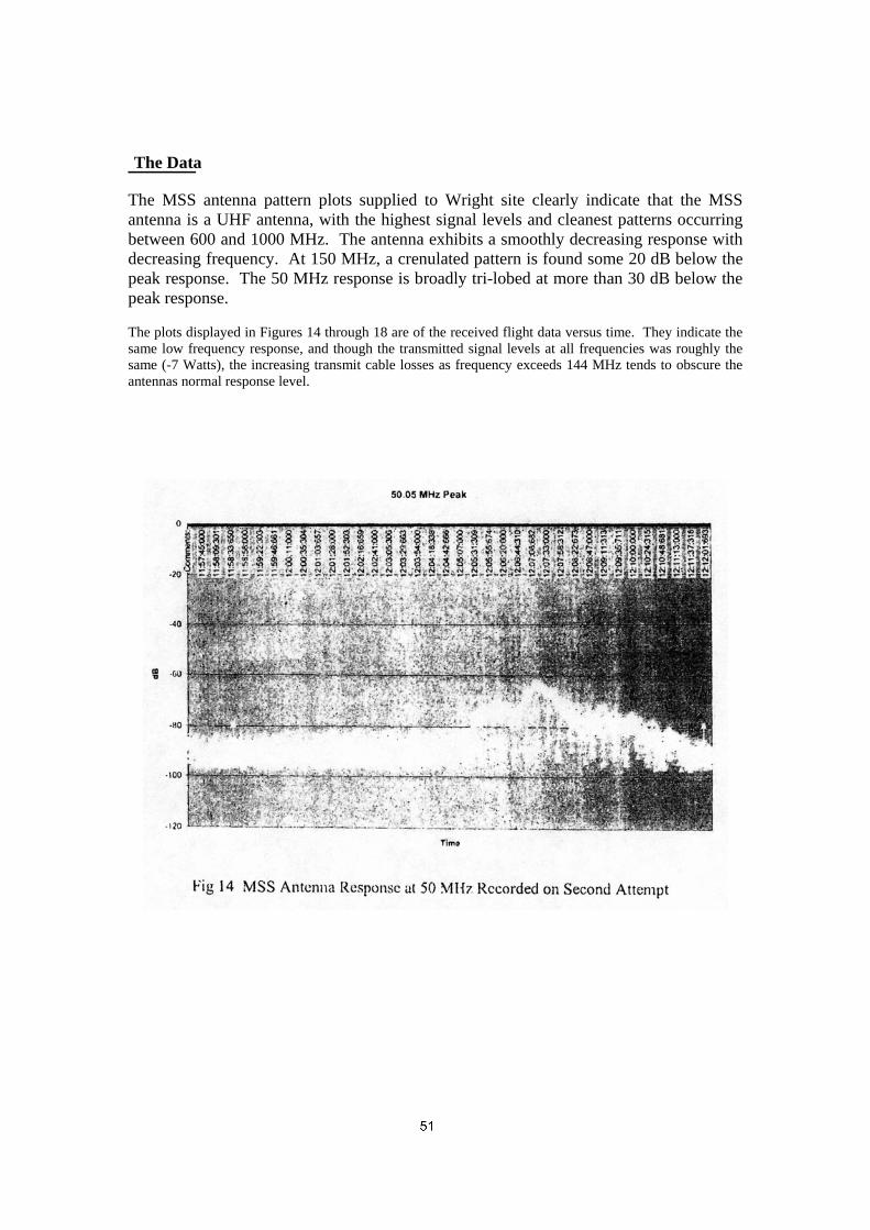
5 1
The Data The MSS antenna pattern plots supplied to Wright site clearly indicate that the MSS antenna is a UHF antenna, with the highest signal levels and cleanest patterns occurring between 600 and 1000 MHz. The antenna exhibits a smoothly decreasing response with decreasing frequency. At 150 MHz, a crenulated pattern is found some 20 dB below the peak response. The 50 MHz response is broadly tri-lobed at more than 30 dB below the peak response. The plots displayed in Figures 14 through 18 are of the received flight data versus time. They indicate the same low frequency response, and though the transmitted signal levels at all frequencies was roughly the same (-7 Watts), the increasing transmit cable losses as frequency exceeds 144 MHz tends to obscure the antennas normal response level.

5 2
Fig. 15 MSS Antenna Response at 144 MHz
Fig 16 MSS Antenna Response at 432 MHz
Fig. 17 MSS Antenna Response at 902 MHz
Fig. 18 MSS Antenna Response at 1296
MHz