a brief review of probability, bayesian statistics, and ...mturk/ml/misc/frey probability...a brief...
TRANSCRIPT

A Brief Review of Probability,
Bayesian Statistics,
and Information Theory
Brendan FreyElectrical and Computer Engineering
University of [email protected]
http://www.psi.toronto.edu
�

� � � � ��� ��� � �
� A system is described by a set of random variables� ������ ��� ��������� ��� � with domains � ��� � � ��������� � �
� A configuration is an assignment to�
� A sample space is the set of possible configurationsand is given by the product of the domains:� � � � � � � ������� � �
Ex: A die. � �. � � �
� � �������!�#"�$ (# of dots on die)
Ex: 2 dice. � %. � �
� � � � ���������&"'$ .� �(� ���������&"�$ � ���)� � �*� � �)� � %+� �������,� � "-�&" � $
Ex: 2 dice. � �. � � �
�(� ���������&./"�$ . Less untuitivethan above.
Ex: 2 dice, angle of hand. � . . � � � � �(� ���������&"�$ ,
�10 �32 4 5 6(7 8 2 9 %;: $
�

��� � ��������� � � �!� � �� � �The probability of configuration
�, � ���'�
, is a real numberthat satisfies
� 6 7 8 � ���'� 8 � � ����� � � �'� �
Ex: 2 unbiased dice. � ���'� ��� ./" , for� � � � �3� ����� � " �#" � .
��� � ��������� � � ������� � � � � ����� � � � � �The probability density for configuration � , � � � � , is a realnumber that satisfies
� 6 7 8 � � � � � � ��� � � � ��� � � � � �
where� � � � is a differential volume of � .
NOTE: � � � �! �is possible.
�#" � $ � ��� � �%� � � � � � � ����� � � � �
1� � � 6 7 8 � � � � � � � � � � � � � � ��� � � � � �
0
� � � � � " � � � ��� � � � � � � ��� � �!� ��� � �
A random experiment or simulation produces aconfiguration
� 4 � .
Discrete case: In�
experiments, the fraction of timesconfiguration
�occurs converges to � � �'�
as� � �
.
Continuous case: Suppose � � � is a region of � . In�
experiments, the fraction of times a configuration in �occurs converges to
� � � � � � ��� � � � �as
� � �.
�

� ���������������� ��������������� ������ ������� �������������� ������ ������ !�����#"
� � � �%$-� is the probability of � given the value of$
� Imagine throwing away all experiments where$
is notequal to the given value
& �����'�(�������)��*+�
� and$
are independent if � � $ 6 � � � �%$-� � � � � and
� ��$ � � � � ��$-�
� Knowing$
tells us nothing about the value of � andvice versa
,

� ������� ���� � � � � � $-� � � � � $-� � ��$-� � ��$ � � � � � � � and ingeneral, � ����� � �
��� � � � � � � � � ��������� � � ��
� If � and$
are independent,� � � � $-� � � � � $-� � ��$-� � � � � � ��$-�
� ��� ������� ������������� ����� � ����� �������������� ������ ���)�� ������"
From the chain rule and normalization,� � � � � $-� � � ��$ � � � � � � � � � � �� � � � � is sometimes called the marginal of � � � � $-�
For densities, � � � � � � $-� � $ � � � �
�

� � � �) ���� �Since � � � � $-� � ��$ � � � � � � � � � � �%$-� � � $-�
,
� � $ � � � � � � �%$-� � � $-�� � � � �
Using � � � � � � � � � $-� � � � � � $-� � ��$-�,
we get Bayes rule
� ��$ � � � � � � �%$-� � ��$-�� � � � �%$-� � � $-�
� For � observed and$
hidden, we call � ��$-�the prior,
� � � �%$-� the likelihood and � ��$ � � � the posterior
For densities,
� � $ � � � � � � �%$-� � ��$-�� � � � � �%$-� � ��$-� � $
�

� � �(�)*+�!� �� ���The expected value of � is
� � ��� � � � � � � � � � ��� � ��� � � � � �� � can be a vector, eg,
� � � � ��� � � � ��� � � � � �� � � � � $ � � � ���� � � $ �� � �� � � � � � � � � � � � � , or � � � � � � � � � � �
� ��� � ����* � �� � *+�� ���
The variance of � is
��� � � ��� � � � � � � ��� ��� � � � � � � � � � � ��� �
�� �
��� � � ��� � � � � � � ��� ��� � � � � �
� If � and$
are independent,��� � � � � $ � ��� � � ����� ��� � � $ �
�

� ������� � ����* � �� ��� � !* �� ���
The covariance of � and$
is��� � � � � $ � �
� � � � � � � ��� �!��$ � � � $ � � � � � � $-�� If � and
$are independent,
��� � � � � $ � 7(not vice versa)
� In general,��� � � � � $ � ��� � � ����� ��� � � $ �� % ��� � � � � $ �� ������� � ����* � � � � � � � �� � �)* � ��� ����� � ���� �)
The covariance matrix of�
is��� � � � � � � � � � � � � �!��� � � � � � �� � � ���or, for � 4 5 �
,��� � � ��� � � � � � � � ��� ��� � � � � ��� � � � � � � �
�

� � � � � ��� � � � � � � � � � �!� ���
� 4 �37 � � $ (eg, coin toss)
� � � � � � � � � � � � � ���� � � � �� � � � � 7 �
where� 4 � 7 � � � is the probability that � is 1.
� Sometimes, we parameterize�
using� ���-� � � ��� � 2 � � , 2 4 � � � � � �
� � � ��� 7 � � � � � � ��� �� ��� � � ��� ��7 � � � � � � � � � � � � � � � � � � � � � � �
� �
� � � � � � � � � � � � � � � � � ��� ���
� 4 5(eg, prior for the probability that a coin will land
heads up)
� � � � ���� ���-��� � �
��8 � 8 �
7otherwise
� � � ��� �� � ��� � %
� ��� � � ��� ��� � �� � �'�*%
� �

� ����������� ������� ��� � ��� � �������������������
Machine learning and statistics study how models arelearned from data.
In Bayesian machine learning and statistics, the model isconsidered to be a hidden variable with a priordistribution. Given the data, the posterior distribution overmodels can be used to make predictions, interpret thedata, etc.
Maximum likelihood (ML) estimation and maximum aposteriori (MAP) estimation can be viewed asapproximations to Bayesian learning, where the mostprobable model is selected. (In ML estimation, the priorover models is assumed to be uniform.)
��

� � � �������� � � � � �� � � ��� � ����� ��� ����� ���� ��� ����� � �
Suppose we flip a coin a bunch of times and see ��heads and �� tails. In a “frequentist” approach, weestimate the probability of heads as
�� �
�-� � � ��
� �
In the Bayesian approach, we first specify a prior, say thatthe probability of seeing a head, � � � � is uniform on
� 7 � � � .Using Bayes rule, we obtain
� � � � � � � ��� � ��� �)� � � � ��� �which is a Beta distribution with mode �
��� � � ��
�and
mean� � � �*� �-�
� � �� � %+�.
This distribution can be used to make decisions, computeconfidence intervals, or interpret the data.
For example, the minimum squared loss estimate of�
is�� �
� � �3� �-� � � �� � %+�
This is closer to the prior than the frequentist estimate.
� 0

� � � � � �
Entropy is a measure of the maximum average amount ofinformation that a random variable can convey in its value
The entropy of a discrete variable � 4 �(� � % ����������� $ is
� ��
� � �
� � � ������ � � � � � bits
� For a discrete variable,� 7
since � � � � 8 �
� The more uniform � � � � is, the greater the entropy
� If � ���� � � � � � is an integer for all � , bits of informationcan be conveyed using an encoder that uses
� � � � � ����� � � � � �bits to pick �
� If� ���
(natural logarithm) is used instead of����� �
,information is measured in nats.
� �

� � � � �� � � ����� � ��������� � ����� � ���� � * � � � ������* � �!�)
� � � � � � � � � String
1 0.5 1 0
2 0.125 3 100
3 0.125 3 101� �
� � � � ��� ��� � � � � �4 0.125 3 110
2 bits
5 0.125 3 111
Imagine we have a queue of random bits (eg, acompressed image) that we’d like to convey.
We can use this information to produce a series ofexperiments for � . Each experiment is produced thus:
� Draw a bit�
from the queue
� If� 7
set � �and terminate the experiment
� If� �
draw two more bits and use these to pick�
2, 3, 4 or 5 and terminate the experiment
This procedure picks � according to � � � � and conveys anaverage of
7 ��� � � � � � 7 � ��% � � . %bits per experiment
� ,

� � � � � � � � � ��� � �
Instead of encoding a bit string into a random variable � ,we can encode � into a bit string using a source code.The decoder uses the bit string to recover � .
It turns out that if � has a distribution � � � � then theminimum average bit string length is
� ��
� � �
� � � ��� ��� � � � � �
� If � ���� � � � � � is an integer for all � , the minimum canbe achieved by mapping each � to a bit string withlength
� � � � � ����� � � � � �
� �

� � � � � � � � � � � � � ����� � � � �!� ���
� 4 �37 � � $ (eg, coin toss, bit from a magnetic disk),� � � � � � � � � � � � �
where� 4 � 7 � � � is the probability that
� is 1.� � � � � � ��� ��� � � � � �
� �)� � � ��� ��� � � � � � � � � ���� � �
0
0.1
0.2
0.3
0.4
0.5
0.6
0.7
0.8
0.9
1
0 0.2 0.4 0.6 0.8 1
Ent
ropy
of B
erno
ulli
varia
ble
Probability that Bernoulli variable equals 1
-x*log(x)/log(2)-(1-x)*log(1-x)/log(2)
� �

� �) � ��� � � �)��� ������ ��� �� ����*������ �)� �� ��)� ��� � �'� � �)��* ��"Relative entropy is a measure of the average excessstring length when the wrong source code is used.
� Suppose the true distribution for � is � � � � , so theminimum average string length is
� ��
� � �
� � � ��� ��� � � � � �
� Suppose we use bit strings determined from thewrong distribution, � � � . The average string lengthwill be
� ��
� � �
� � � ������ � � � �
� The average excess string length is the relativeentropy :
� � � � � � � � � � � ��� ��� � �� � �
� � � 7
� �
� ��� ����� � � � � ��� � � � � � � �������!� �
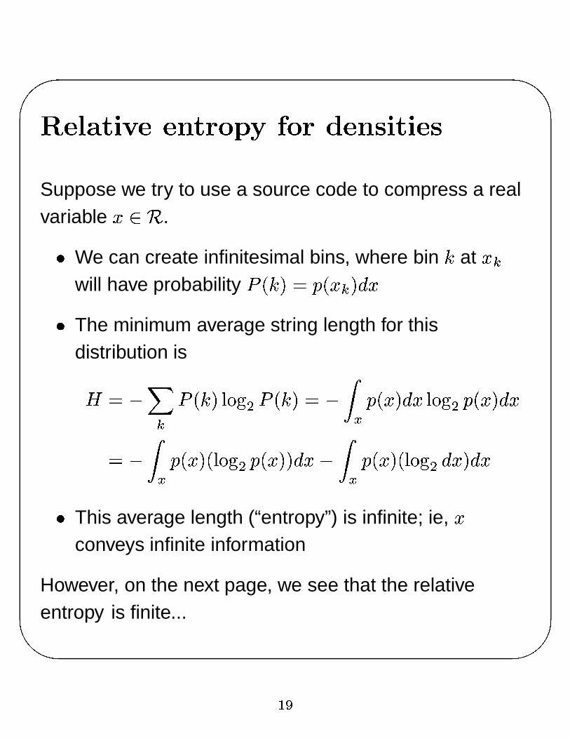
Suppose we try to use a source code to compress a realvariable � 4 5
.
� We can create infinitesimal bins, where bin � at ���will have probability � � � � � � ��� � � �
� The minimum average string length for thisdistribution is
� ��� � � ��� ��� � � � � � � � � � � � � � � ��� � � � � � � �
� � � � � ��� ����� � � � � � � � � � � � � � ��� ����� � � � � � �� This average length (“entropy”) is infinite; ie, �
conveys infinite information
However, on the next page, we see that the relativeentropy is finite...
� �

� �) � ��� � � �)��� ������ ��� ���)�� !������� *+�������� ���)�Suppose we use bit strings determined from the wrongdensity �
� � � . Under this density, bin � at � � will haveprobability � � � �
� � � � � � .
The average string length is
� ��� � � � ������ � � � � �
� � � � � ��� ����� � �� � � � � � � � � � � �!� � ��� � � � � � �
The relative entropy (excess average string length) is
� � � � � � � � � � � � ����� � �� � �
�� � �
� �� � � � � 7� Since the relative entropy is finite, we refer to
� � � � � � ��� ��� � � � � � � �as entropy, although it may be NEGATIVE!
� �

" � � � � � � ��� � � � � � � � � � ��� ���
� 4 5(eg, distribution of failure times)
� � � � �������� �� � � 77
otherwise
� � � ��� ��� �� ��� � � ��� ��� � �� � � � � �
�� ��� ����
� ��, �
�
� � � ��� � � � nats ���� � � � � bits
� The entropy increases as��� � increases
��

� � � � � ��� � � � � � ����� � � � � � �� � � �!� ���
� 4 5(eg, variable that is a sum of a large number of
other real random variables)
� � � � �
� %;:�� � � �� �� ���� �� �
� � � ���
� ��� � � ��� � �
� � �� ���� %;: � � � nats �� ���� � %;: � � � bits
� The entropy increases as� �
increases
�&�

� ��� � � � � ��� � � � � � ���!� � � � � � �� � � �!� ���
� 4 5 �
� � � � �
� %;:�� � � � � � �� �� � ������ � � � �� �
where 4 5 �
,� �
is an � � � positive definite matrixand
� � � is the determinant
� � � ���
� ��� � � ��� �, an � � � covariance matrix
� 0

� � � ��� �
Suppose we have an invertible function$ � � � and a
density � � � � .� When a small volume is mapped from � -space to$-space, the probability in the volume should stay
constant.
� However, because the volume may change shape,the probability density will change and the Jacobiancaptures this effect.
� Conservation of probability mass gives� � � ��� � � � � ��$-��� � $ � , � � � $-�
and
� � $-� ����� � � � � � ����� � ��� � � � ��
���� � �
is called the Jacobian
� For � 4 5 �and
$ 4 5 �,
��� �
is a matrix of derivatives
� �

� � � � � � �
� ������������ ������: A. Leon-Garcia, Probability and Random
Processes for Electrical Engineering, Addison Wesley,New York, NY, 1994.
� � � �) ��� � � ��*���� ��� � � ��� ��� � � ����� � �!� ���� ���* : R. M.
Neal. Bayesian Learning for Neural Networks, Springer,New York, NY, 1996.
& � ��� � � �� ��� � ��� �����: T. M. Cover and J. A. Thomas,
Elements of Information Theory, John Wiley & Sons, NewYork, NY, 1991.
� � � � � � � ����� ������ �) �� * �� �* �� ��� ����� ��� ���)� �� � �� ��� ��* � :
Useful when we study Gaussian models.
http://www.psi.toronto.edu/matrix/matrix.html
� ,