a brief history and development of ‘real value’ valuation

1

A BRIEF HISTORY AND DEVELOPMENT OF ‘REAL VALUE’ VALUATION MODELS – THE LAST FOUR DECADES

A paper prepared for presentation at the Pacific Rim Real Estate Society Conference, Sydney, Australia,

18-21 January 2009

Rodney L Jefferies

Farm Management and Property Department, Commerce Division, P.O. Box 84, Lincoln University,

Lincoln 7647, Canterbury, New Zealand

Corresponding author: [email protected]

Abstract

This paper summarises the author's research of the literature related to the concept of ‘real value’ valuation models as applied to income or investment property which transpires to be, on one hand interesting, but on the other-hand disappointing in their scope and lack of adoption by the valuation profession.

The basic real value valuation model was promoted in the UK as a "positive" investment valuation model in the early 1970's. However, it foundered in the 1980s due to the rejection of the (then) complicated formulary and mathematical calculations required in favour of a more recognisable nominal ‘equated yield’ valuation model.

To a lesser degree and in a different format, a not dissimilar "dynamic capitalisation" valuation model was promoted in the 1980s in the USA. That model also appears to have similarly foundered in favour of the (then) well established ‘mortgage-equity’ appraisal model then in use since the 1960’s.

The author has, over the last decade, further developed a more contemporary and adaptable ‘real value’ valuation model that differs in some important aspects from these UK and USA models particularly in its user-friendly spreadsheet template model format with a flexibility that hopefully will not suffer the same ultimate oblivion as these earlier models.

Keywords: dynamic capitalisation, equated yield, income capitalisation, inflation, leased fee, leasehold, positive valuation, real required returns, real growth, real value, reversionary freehold, short-cut DCF.

No of Words: 15529

mailto:[email protected]

R L Jefferies − A brief history and development of ‘real value’ valuation models

2

Introduction

This paper is as much an autobiographical academic journaling as it is a brief history of real valuation models. In effect it compares the author’s attempts at rationalising the challenge of inflationary growth as it affected valuation theory and practice in New Zealand in the 1990’s, as it contrasts those efforts with other solutions unbeknown to the writer at the time, having previously been instigated in the United Kingdom and the United States in the 1970/80’s. The latter efforts had largely gone unrecognised and ignored by mainstream property professionals as well as the valuation/appraisal fraternity and in the UK formally rejected by the RICS. To now suggest that the use of real value valuation models are a superior technique, especially “in the face of strong winds” from off-the-shelf DCF based investment valuation and analysis “black-box” software technology almost universally adopted internationally by valuers and appraisers, may seem foolhardy – but that is just the role academics are renowned for if worthy of the affectionate description as “gurus” or “gods” by students past and present.

The impact of inflation and its inter-twining with growth in real v. nominal terms was a problem that concerned the writer, when authoring the standard NZ valuation text (Jefferies, 1977) during the late 1970’s as conventional direct capitalisation income valuation models did not recognise how to deal with it in a rational and technically sound manner.

It escaped the writer, (being a practitioner turned lonely academic) as to how to deal with it later when writing Vol II and revising the 2nd Edn of the original Vol. I text at the turn of the 1989/90 decade and resulted in “stink thinking” that permeates the capitalisation techniques then espoused − still used as the ‘valuation bible’ in NZ (Jefferies, 1978, 1990 & 1991). It was not till the early 1990’s that the writer was exposed to the influence of academic challenge from the emerging property finance branch of land economics that the (late) Dr Gerald Brown1 brought to New Zealand and supervised the writer’s post-graduate study – when the “light went on”.

This resulted in a struggle to incorporate logical and practical ‘real value’ solutions into property investment valuation techniques, especially in the valuation of lessor’s and lessee’s interests of both occupational and ground leased properties. That lead the writer to the development of ‘real value valuation models” (Jefferies, 1997a, 1997b).

It was therefore something of a shock to find this was not actually original research (though it was to the writer), when Dr Neil Crosby kindly referred the writer to his and Dr Earnest Wood’s earlier PhD research and work in the UK. Subsequently, and somewhat serendipitously, the writer “stumbled” over what seemed parallel (and seemingly ignored by academics) practitioner and actuarial based research in the USA by Gordon Blackadar2 who developed a dynamic capitalization model that he had published in the 1980’s – the only fully developed version of a real value valuation model the writer has found in that continent’s vast appraisal literature.

This paper contrasts these independently developed models from two islands at the opposite sides of the world and a continent in-between in the hope that others might re-look at the merits of the real value models as a possible viable alternative to the creeping virus of inflationary based DCFs.

At the time of writing, one wonders to what extent reliance on inflationary based DCF valuation models have contributed to the economic and financial meltdown of global asset markets now

1 Brown, G. R. (1991) – Gerald was the Founding Professor of Property at The University of Auckland in 1991 – 1994 who died in 2004 and is remembered by quite a few students for whom he patiently waited for the “light to come on”. 2 Blackadar, C. G. (1984)


3

facing the devastating opposite effects of prospective declining values, currency deflation and potentially depression (unless world-wide financial rescue packages are successful).

The world has changed and will not be the same, though similar déjà vu times of recession, deflation and property investment “busts” will lead to recriminations, as in the 1980’s & 90’s, to a serious questioning of the suspected ‘stink thinking’ in investment valuation methodology and looking to the scapegoat valuers and appraisers to lay some of the blame on. Is there, again, a case for “real value” for “real estate” valuations as the basis for moving forward into the 21st Century’s property investments and valuations thereof? Is this the answer or ‘wishful thinking’?

The basic real value valuation model

The fundamental and underlying simplification of how property investments are valued under a real value concept is that the current market value of an investment property is the real present value of all future ownership benefits. As familiar as this basic, even trite, doctrine will be − it is also axiomatic that in real terms the market price of an asset at the date of valuation will be represented by what buyers and sellers agree to exchange those property asset interests in current dollar terms, i.e. representing what other real things can be exchanged for that current monetary value.

Current market rentals will represent in real terms what the periodic occupancy benefits are worth both now and in the future, the latter requiring those future real values to be discounted to present value at a real discount rate. Similarly, current and future expenses and capital expenditure, as well as any future net resale value, can similarly be expressed in current present ‘real value’ terms. This simplifies the valuation process, in that it is not necessary to escalate (or inflate) future rents, costs and values in nominal terms allowing for currency inflation, and then to discount those future values back to present value at a nominal discount rate that necessitates incorporating the same expected inflation component. One needs only to discount the forecast future real cash flows using real required rates of returns, allowing for relative risks.

This does not mean that monetary inflation is ignored, but is specifically allowed for by taking it out of the nominal monetary discount rate; nor does it mean that one ignores real growth (or decline3) provided that is forecast in real terms and also specifically allowed for by taking it out of the nominal monetary discount rate to derive a net of inflation and growth expected ‘real rate’ of return. Only when there is a real prospect of real growth in rentals and values resulting therefrom − will the forecasts require adjustment for that expectation, and vice-versa for real value decline (such as that due to depreciation and/or obsolescence, demographic shifts or effects of changes in demand/supply). Traditional methodology inherently makes these allowances implicitly – while DCFs do so explicitly in future nominal currency terms. Real value models takes out the difficulty of forecasting inflationary expectations and their offsetting “in and out” compounding and discounting effect, which if correctly and consistently executed is of neutral effect on present values – so why do it?

The writer4 describes his model as “... treats known contractual rental income conventionally as an ordinary annuity discounted at an inclusive of growth investment yield rate. The real value model bases forecast rental review income and reversions on expiry or terminations of leases in “real terms” and discounted these at a “net of inflation and growth” investment yield rate.”

3 In terms of the building value component this will be any real depreciation due to age and obsolescence, arising from the reduced ability to command the market in competition with new or newer space. 4 Jefferies, R. L. (1997a)


4

The complications facing a valuer or appraiser in conventional capitalisation techniques relate to deal with contract rents being less than market, i.e. under-rented; conversely over-rented properties; valuation dates other than at the point of a rent review; vacancies and lease-up costs; exceptional costs or required capital expenditure; differing growth rates in income of various components of the property and/or various expenses; or uncertainty as to the likely holding period; etc., and require adjustment techniques. However, these are simplified to the extent that each of these adjustments are carried out in current real terms, and discounted to be reflected in either positive or negative contributions to present real values.

Gordon Blackadar (supra) expresses this concept succinctly in the subtitle of his paper as "an income approach in real dollars at real interest.”

Earnest Wood5 expresses this as "an approach which accepts the norms and conditions of society that real property values and returns may remain constant or may change, in real terms”.

Neil Crosby6, challenged the widely held view in the field of property investment valuation "that conventional valuation techniques are adequate for assessing the market value of investments.” He argued that the standard UK equated yield models are "… more explicit regarding future income changes, but that the formula involved are more complicated than in the real value technique.” Further, he points out7 that “the Real Value approach looks at income in terms of its purchasing power.”

The common problems expressed by these two UK writers are that the traditional and conventional approaches of direct capitalisation and discounted cash flow techniques are hampered in terms of reliability and usefulness by the impact and uncertainty of inflation. The valuation philosophy and methodology of those (UK) conventional techniques are not structured to recognize and cope with the subtleties of value change in real and inflationary terms and their consequences.

Earnest Wood8 in the preamble to his thesis states that "...it is not just the measuring rod of money which has become distorted so that it cannot perform its functions but often the methods of valuation, being based on invalid tenets, are not calibrated to deal with the situation".

If there is a paradigm shift to the adoption of real value models the end result should be simpler and more accurate investment property valuations – but comparable to well executed fully explicit DCFs. The latter models are unlikely to be supplanted where detailed period-by-period forecasts are required – but in many cases they are not – and can lead to the inevitable exposure of errors in with ex-post comparisons of conventional DCFs nominal forecasts with actual outcomes. Any future event will be subject to Jefferies’ Law – that “whatever you predict is far more likely to be wrong than right!”. The chances that a valuer’s explicitly estimated reversionary or terminal (exit) value is “on the button” or near it will be more than a fortuitous combination of offsetting errors!

As real value models are firmly fixed on the reality9 of current (real) values makes the chance of being exposed ex-post in the future for ex-ante errors in real growth and inflationary expectations

5 Wood, E. (1972) p15. 6 Crosby, N. (1985) 7 Crosby, N. (1983) 8 Wood, E. (1972) where in Part II Chapters 8 to 11 he sets out the axiomatic “formulation” of his model. 9 That applies equally to rentals, expenses and asset values under the axiomatic land economy anticipation principle reflected in the market (not the valuers forecasts) having already discounted all future expectations into present value comparative and comparable evidence. Valuation is not a science but an art and accuracy is not guaranteed as “Real estate values are not crystals on which we cut sharp edges. We do not prove our conclusions, we support them” (Blackadar, 1989, p.340)


5

“hidden” in the discount rate. This should be of comfort to any valuer and probably the model’s greatest comparative advantage over traditional and DCF valuation methodology – especially as the latter’s explicit presentation in last digit pin-point accuracy invalidly implies.

UK Real Value Models:

These were first heralded in the UK by Earnest Wood10 as a "positive" investment valuation model in the 1960's.

Earnest Wood’s Real Value Model emerged from his PhD research (Wood, E. 1972) when he first published a series in three weekly Parts in the practitioner‘s Chartered Surveyor magazine (Wood, E. 1973). The first and second Parts are a ‘warm-up’ to set the scene for his introduction in the third Part of his real value model concepts, definitions, and formulae. He is critical of earlier models being based on an inflation prone yield, whereas his real value model is based on an inflation-risk-free-yield (IRFY) an abbreviation also applied to his model. He defines the IRFY as a ‘yield excluding inflation and real value change’.

It was one of the earliest and most challenging articles that addressed the problems caused by inflation in dealing with the traditional valuation of investment property in the UK. It appears, with hindsight that Wood’s concepts and model were beyond the readership to grasp let alone apply.

The problems then emerging with contemporary and traditional United Kingdom ARY (all risks yield) capitalisation models − relying on calculating investment value by applying a YP (year’s purchase) to a static net rental allowed improperly for the effects of rising inflation – were largely being met by the promotion of discounted cash flow techniques using a redemption yield (Greaves, M. J. 1972). Competition came from and lead to the adoption of a competing EY (equivalent yield) valuation model. This had been originated by Phillip Marshall (Marshall, P. 1976) and codified by him into his published pre-computed Donaldson’s Investment Tables (2nd edn) (Marshall, P. (1979).

The EY model was easier to understand, at least to the professional establishment, and Earnest Wood accused Robert Clark, the Research Director of the Research Project into Property Valuation Methods commissioned by the Royal Institution of Chartered Surveyors (Trott, A. J. 1980, 1986), of promoting it as a protagonist of EY (Clark, R. E. 1978).

Wood’s somewhat bitter reaction (Wood, E. 1986) to the report’s rejection of his claimed superior model in favour of the EY model’s adoption as the recommended standard by the RICS makes most interesting reading. He reproves11 the report’s authors for recommending a model that he shows relies on an inflation prone redemption yield as its target yield.

However, access to Wood’s research was and still is (largely) restricted to those who can visit Reading University and read it in the library archives12.

A précis of Wood’s contribution to real valuation modelling and summary of his basic formulation with an example is set out in the attached TABLE A – along with the other real value models discussed in this paper.

10 Wood, E. (1967) p 197, where 5 years earlier, he identified that the “true yield will be the initial yield minus the rate of inflation” but he had not then developed his real value model to solve the fundamental issue of: “What are the frames of reference to which the true yields should be related?” 11 It may have also reflected some academic rivalry at the time Wood being at Reading University and Trott & Clark at the Polytechnic of the South Bank in London 12 The author put a restriction on his thesis being consulted and copied. This writer, 36 years later, had great difficulty from New Zealand over 9 months to negotiate a partial release of that restriction to obtain a photocopy of partial extracts. In total it is in two Volumes and 806 pages!


6

Dr Neil Crosby’s Real Value Hybrid Model was developed in his PhD thesis13 (Crosby, 1985), the model’s concepts first presented in a RICS Junior Organisation Prizewinning Paper (Crosby, 1982) and more concisely expounded in two series of articles and a reply first outlining the real value approach in the Journal of Valuation (Crosby, 1983, 1986a); followed by a technical and application series (Crosby, 1986b).

This advanced model sought to bridge the gap between Wood’s model and the EY model championed in the Trott reports, by overcoming the criticisms of the complexity of Wood’s model while using the familiarity of the traditional methods incorporated into the EY method and expressing this in a short-cut DCF format. This was quite a feat and Crosby gave it the (elongated) name “real value equated yield hybrid method” though later descriptions changed to a less confusing “real value/short-cut DCF hybrid” model (Baum and Crosby, 2008).

This model splits a leasehold investment’s (reversionary freehold; leased fee or lessor’s interest) rental cash flow into two tranches using a “term and reversion” format:

(i) The rental term to the next review being “capitalised” (discounted) using a Year’s Purchase (YP) (reciprocal of a capitalisation rate) based on an equated yield (overall nominal discount rate including growth); plus

(ii) The rental reversion (to market) taken as at the next review date based on: a. the current market rental value – CRV – at date of valuation (not as at reversion

date), taking into account the rent review frequency; b. capitalised at the current reversionary YP (market capitalisation rate); and c. discounted to present value at a real yield (real discount rate, i.e. net of any

inflationary growth assumption, i.e. a IRFY).

The sum of these two present values gives the current leasehold investment’s value (reversionary freehold; leased fee or lessor’s interest).

However, the reversionary freehold (current market investment value – assuming newly or recently leased at CRV) is technically valued in the same manner – but as the reversion is co-incident with the valuation date, (i) above is zero and the calculation simplifies to simply (ii) (a) plus (b) above only, i.e. not discounted as in (c) above.

The model produces the same current valuation as a period-by-period fully explicit DCF (or a short-cut DCF) where nominal currency cash flows are forecast to the reversionary date and the then rental forecast at the assumed growth rate is capitalised at the market capitalisation rate (ARY) and all cash flows discounted at the EY (nominal discount rate including allowance for growth) to present value.

The main cogent argument for using the real value hybrid model over the traditional UK ARY model is that the latter over-values the term (as it capitalises or discounts the rental cash flows at the initial capitalisation rate); and undervalues the reversion (as it capitalises the current rental value and discounts that at the capitalisation rate). This makes no difference to the result for a reversionary freehold (fully let recently lease property) but significantly undervalues the leasehold investment value (lessor’s interest) despite some offsetting of those errors – which increases as the term to run increases and significantly so for long or renewable leaseholds).

13 An extensive work also of two Volumes and a total of 1034 pages – available on microfilm from the British Library. He was (then) a student at Reading University and clearly relied on Wood’s model and developed it further.


7

A précis of Crosby’s contribution to real valuation modelling and summary of his basic formulation with an example is set out in the attached TABLE A – along with the other real value models discussed in this paper.

Demise of the UK real value models.

These UK real value models foundered in the 1980s due to the rejection of the (then) complicated formulary and mathematical calculations required in favour of a more recognisable nominal ‘equated yield’ valuation model. The interim Property Valuation Methods Report summarised that Wood’s method “…has suffered from complexity. A valuation technique, if it is to be accepted by the profession, must be easily understood and easy to use – Its theoretical soundness must be matched by a practical application” and concluded that “It is considered that Dr. Wood’s “Real Value” approach is too complex for most practitioners to be able to use in their day to day work and that the more practical and simple equated yield analysis be used in preference” (Trott, 1980, p.56 & 57). This view was confirmed in the final report in that the “Wood (method) and Bowcock (method) are too esoteric and the use of the complex formulae which their methods involve is likely to act as a deterrent to the every day practitioner” (Trott, 1986, p.101).

The Mallinson Report (RICS, 1994) following the boom/bust of the UK property market in the late 1980’s and early 1990’s made a number of far reaching recommendations affecting how valuations should be undertaken, presented and justified by the valuation profession in the UK.

Mallinson’s recommendations 24 and 25 related to the development of modified ARY and DCF techniques, reducing dependence on the ARY method and codifying and disciplining the latter with new Guidance Notes. A working party undertook a survey of practitioners in the market as to the then adoption of conventional/traditional or contemporary/DCF methodologies in undertaking valuations (French, 1996) and this showed few (5% of respondents) using real value methods for reversionary freehold or over-rented properties only, against a dominance of reliance on ARY or EY methods.

This lead to the publication of an RICS Information Paper on Commercial Property Valuation Methods (RICS, 1997) in which there was only passing footnote references to Wood’s real value method with recommendations on using and examples of the EY and Short-Cut DCF methods.

The latest UK texts continue this emphasis, Douglas Scarrett’s 2008 2nd Edn. of his established text continues to describe the traditional approach with a brief two page reference to real value models in which he acknowledges “Earnest Wood suggested a ‘real value model’ that he promoted with some energy, but it was not taken up” and “Neil Crosby has developed a model that has some of the elements of Wood’s real value and which he describes as a real value/equated yield hybrid.” The IRFY is defined along with an (unexplained) simplistic example of valuing a rack-rented office block using this method (Scarrett, 2008, pp. 107-108).

Sarah Sayce’s, new 2006 text completely disregards any real value methods (Sayce, et al, 2006) as does Peter Wyatt’s new 2007 text both relying on ARY and DCF techniques with little reference even to EY techniques. Wyatt states “…at the present time, there are two recognised approaches to valuing a property using the investment method: income capitalisation using an ARY and discounted cash-flow (DCF) using a target rate of return or discount rate.” (Wyatt, 2007 p.126).

Andrew Baum and Neil Crosby in their 2008 3rd Edn. of their text continue to devote a section to real value models and (as might be expected) including a succinct explanation and worked examples of the “real value/short-cut DCF hybrid model” (Baum and Crosby, 2008).


8

Despite Neil Crosby’s persistence, attempts at integrating real value models into the mainstream in the UK have been thwarted. To an increasing extent the technological advances in computing and DCF programmes with standardised methodology now incorporated into mainstream international valuation standards and guidance notes has replaced the apparent need for real value models, especially where valuing complex and/or multi-tenanted investment properties. Standard UK undergraduate texts such as The Income Approach to Property Valuation (Baum et al, 1979, 1981 and 1997) advocates the benefits of using DCFs but teaches the latter alongside conventional capitalisation approaches as “All income capitalisation are a simplified form of DCF.” (Baum et al, 1997, p.57.) It merely lumps rational and real value methods together – as an alternative basis of discounting without any explanation (p. 55) but gives a brief acknowledgment to Neil Crosby as “the principal exponent of this technique” and half-page overview including a simple example (p. 63).

USA Real Value Models:

Because of the almost standard adoption of the Ellwood mortgage-equity technique as an income property appraisal model since the 1950’s that explicitly forecast growth or decline (as depreciation/appreciation) in capital values over an estimated holding period, alongside equity build-up based on the USA norm of long term fixed interest table mortgages – the “problem of inflation” did not arise as a serious criticism of that model. It did not, however, allow for growth or decline in rental income during the holding period – but later did allow for equity-build-up through the addition of a ‘J-factor’ in the model. The calculations produced an adjusted overall capitalisation rate and were simplified by the provision of tables and charts and the process was also one utilising the early computerised applications available to appraisers in the USA. Fully explicit DCFs, especially with the widespread availability of PCs in the late 1980’s and 1990’s provided a better methodology that is now the normal income property appraisal methodology adopted in that country.

In the United States, as in the United Kingdom in the late 1970s, the problem of inflation and the limitations of the standard USA appraisal “overall capitalisation” or Ellwood techniques were not without recognition.

Lusht (1979) published an expanded version of an article originally in the Spring 1978 issue of the AREUEA Journal that postulated that then appraisal theory encouraged an improper treatment of inflation in estimating the future benefit flows in investment valuation models; and that inflation had a fundamentally negative impact on real estate investment value.

The (then) consensus in appraisal literature was that inflation should not be recognized in future benefit flows i.e. a current price-level assumption was to be maintained. The reasons cited for this position was that recognizing inflation confuses nominal and effective purchasing power; that present value tables did not anticipate inflation; and that its effects are indeterminate or neutral. Appraisals were to measure objective value in present worth and the numbers of current purchasing power dollars (Ring, 1970, p.327); and further, resale value was to be estimated in terms of current dollars not future purchasing power of the dollar (Johnson, 1976, p.159).

The basic Ellwood tables, (then) in widespread use, represented equity-yield models, which did not accommodate annual cash flow changes but did anticipate appreciation (or depreciation) in resale value to be considered, however the latter was in nominal terms (incorrectly assumed in real terms). The standard appraisal text (AIREA , 1978, Ch.8) similarly ignored inflation effects. The inconsistency of the assumption of level cash flows, combined with allowing value change without a corresponding change in those flows was criticised, leading to over- or under-valuation (Nelson and Allen, 1977).


9

Lusht's article appears to be the first dealing in detail with this appraisal problem identifying that the "yield rate" (as used in equity-yield appraisals) was a nominal one based on a risk-free interest rate plus a risk premium. This raised the problem associated with the use of fixed-cost of debt (leverage) that ignored the loss of purchasing power and the risk associated with inflation of the currency. This should have led to anticipated inflation raising the discount rate, as investors attempted to compensate the future loss of purchasing power of debt, evidenced by the rapid rise in market interest rates and yields in the latter years of the 1970s.

The problem related primarily to the discounting of net operating income cash flows during the holding period at the market discount rate including an inflation expectation, which automatically adjusts estimates of future cash flows to current price levels. It was clear that future flows were estimated at current price levels. They would be deflated twice, once by the analyst, and secondly by the market via the discount rate, the result being present value being biased downward.

Lusht fleshed out this biased model, illustrating by a basic single-period cash flow model the correction required when including an allowance for an inflation adjustment in the discount rate, and for growth in cash flows and net cash proceeds at sale. He demonstrated the effects in a NPV after-tax equity-yield model, comparing inflation at a rate of zero (static price levels) to inflation at a positive rate.

The results clearly showed that the absolute effects of inflation were that inflation is not “good" for real estate values; rather, it had a fundamentally negative impact; and that any positive effects of inflation were traceable only to the ability to obtain significant portions of financing at a fixed interest cost. Using simple variations of his unbiased amended real value model, he showed that the specific impact of inflation on investment value depends on the interrelationships of original cost (as it ultimately reflects in capital gains), the debt/equity ratio, the level of depreciation expense, and the tax rates (income and capital gains). He proved that inflation effects on investment value are both measurable and significant.

Lusht’s conclusions were that the practice of ignoring inflation in the interests of "conservatism" is unsound. It failed to recognize that should the inflation rate be lower (or higher) than anticipated, actual yield will move in the correct direction. His model, whilst a real value one (though he did not describe it as such), fell short of being a valuation model for generic application.

Miller and Solt (1996) in a follow-up article refer to subsequent methodologies designed to deal with inflation, including that the following 8th edition of the AIREA text no longer ignored inflation. “An appraiser can consider the effects of inflation in capitalization by expressing the future benefits in terms of constant dollars (adjusted to reflect constant purchasing power) and by expressing the discount rate as a real or un-inflated rate of return on capital” (AIREA, 1983, p.341).

However, the revised text developed neither a theory nor methodology of using real discount rates and real returns. Miller and Solt, however, did present a real rate/real return valuation model, and further elucidated how to develop the appropriate real discount rate, either by building it up from a risk-free rate including allowance for expected inflation per discount period, as well as extracting the real discount rate from market sales analysis. However, an equity-yield rate was derived on an after-tax basis following Lusht’s model. Though acknowledging changes in the real returns, based solely on perceived changes in market conditions affecting the property as being independent of inflation, they did not specifically develop the model to allow for such real growth. The example included presenting the model in a term and reversion format, but only using a period-by-period basis (assumed annually inflating rental tied to the CPI) using constant current values. They concluded that the potential errors in nominal constant dollar valuation methods without allowance for inflation would bias of the valuation downwards, confirming Lusht’s conclusions. The solution


10

was to be found in properly applying a real rate/real return valuation model, which deserves its place as an appraisal tool.

The primarily advantage expressed was that the real rate valuation model offers consistency of adjustments, and simpler mathematically expressed models than growth rate models. As with the Lusht's model, it had limited application − as presented − being an after-tax equity-yield model, not applicable in countries where no presumed typical financing terms or tax rates apply nor where capital gains tax is not the norm. It also dealt only with a fully-leased-to-market property at the date of valuation. The model’s equation was basically a real value annuity formula.

Klemplerer, D. (1979) published a short article in the Real Estate Appraiser and Analyst that looking back is quite profound, being a forestry valuer in whose industry the dealing with valuations and DCFs in real values has a long history. He made a significant (but seemingly overlooked) contribution to the professional appraisal literature in presenting two simple models that in real terms gave the valuation of both terminating and perpetual incomes where geometric growth was distinguished between inflationary and real growth applying a ”real market interest rate, inflation excluding” discount rate. He defined growth as “real annual rate of growth or decline in payments, inflation excluded.” He refers to these concepts being well established in the natural resources and forestry appraisal fraternity and formulations for these special types of geometric series of payments well known as far back as 1931 by stock (share) market analysts (Guild, 1931) and in the 1970’s (Merrett and Sykes, 1979) – the latter work being referenced by Wood in his thesis. Kemplerer did not develop a full real estate investment appraisal model and his formulae assumed a full equity, annually in arrears, terminating series of annual real growth incomes (applied to timber harvests). He did state similar discounting formula could be applied to perpetual payments on either an annual or periodic series basis.

A précis of Lusht's, Miller & Solt’s and Klemplerer’s contributions to real valuation modelling and summary of their basic formulations with an example is set out in the attached TABLE A – along with the other real value models discussed in this paper.

Young, M. S. (1980) in an Appraisal Journal article raised the problem of inflation and valuation in that the impact of the former cannot be met with traditional appraisal methods. However, he saw the problem, and offered a formula but not a solution. His formula, borrowed from the finance literature in dealing with ‘growth stock’ valuations failed to distinguish inflation (in currency terms) from real value growth (in real terms) as these combine to give a total nominal growth rate. An obtuse reference to the Petersburg Paradox and its use in leading to a real value formula based on a terminating DCF type series of growth incomes is similar to that proffered by Klemperer. He was worried that’s its application would cause a greater paradox − in that where the inflation (growth) rate was close to or equalled the discount rate then very large values tending to infinite values would result, hence the discount rate must be greater than the growth rate.

More enlightening was the response of Brown and Johnson (1980) that criticised Young’s model and conclusions, arguing that there was no paradox when correctly distinguishing real returns (after depreciation due to money inflation) and partitioning the yield into the expected real return and expected rate of inflation – linking this to Irving Fisher’s famous equation. They contributed further by providing a formula where the growth in income is different from the general inflation incorporated into the discount rate and presented an adjusted conventional formula for that method. This was an advance in real value valuation modelling, but similar to Klemperer’s had its limitation to apply as it was not a fully developed real estate valuation model.

The most comprehensive but largely ignored real value valuation model published in the United States was Gordon Blackadar’s Dynamic Capitalization Model which approached the problem from


11

an actuarial viewpoint14 which used international actuarial notations (IAN) and nomenclature and is very complex despite its painstaking explanations. It was published over a discontinuous and lengthy three-part series in The Appraisal Journal (Blackadar, .1984, 1986, 1989). It is worthy of further detailed consideration because of the insights it gave and the help it provides in further developing a contemporary real value valuation model, though he did not describe it as such,.

The first article (Blackadar, 1984), originated from being development in 1980, and first published in a booklet with supplements in 1981-1983. This article sets out the basics of the dynamic capitalisation model, expressed as an "equation of value" and gives a worked example.

It presents an interesting historic setting tracing the history of compound interest from the Greek mathematician Euclid circa 300 BCE, this article, being written after the boom and bust of the 1970s. The core of the paper deals basically with the impact of inflation on property values and links appraisal to actuarial concepts of real present value but the use of IAN notation, definitions, etc., that are strange to appraisers and valuers and off-putting to the professional readership.

Herein lies a practical problem15 with this model − the appraisers' and valuers' difficulty in understanding and thus adoption of the model due to its use of actuarial concepts, derivations, nomenclature, terms and the resulting actuarial functions and equations!

Conceptually, it applies precise ideas and cash-flow conceptual approaches using accurate, but complex actuarial formula applied to appraising income investment grade real estate. At the time the original booklet was published it was quite an independent "real value valuation" model16, but not described as such by the author in those terms but the articles sub-title says it "An income approach in real dollars at real interest". With great care but complexity it deals precisely with the effect of currency inflation separately from real value depreciation and/or growth (appreciation) in rents/asset values, expressed as a continuum in a "varying annuity function" during an asset's life or holding period.

To that extent it was a significant "new" approach in the United States. It had, however, to be somehow linked to be appraiser's terminology and methods/models of the day i.e. capitalisation. Mathematically it does not produce a capitalisation rate. The varying annuity factor in effect is an income multiplier (i.e. YP in UK terminology) applied to a stabilised effective gross income with property expenses not deducted but adjusted for in the income multiplier. This makes the resulting multiplier difficult to compare with an overall yield or capitalisation rate applied to normalised net operating income (NOI).

Dynamic capitalisation is presented as a "function" not a specific equation, though its application uses a variant of a short-cut DCF or discounted future value approach in real terms. There may be different and therefore variable equations that necessarily reflect the dynamics of the investment market and a particular property's characteristic. Thus, the author does not provide a specific or generic valuation formula.

Despite the authors claim (page 593) that "it is desirable to keep equations simple...the examples are fairly simple forms" this reader struggled with the math and a typical appraiser/valuer would be

14 The author, whilst a real estate appraiser, worked in and with the life insurance industry, in New York a Vice-President of Metropolitan Life Insurance Company. Interestingly, Ellwood had a similar professional background. 15 It is a very hard and laborious read. A footnote on the author's background indicates it was “presented” at a 30-seminar at the University of Wisconsin sponsored by Dr James Graaskamp. The writer having experienced the intensity of sitting under Graaskamp’s tutelage in 1973, appreciates how intensive and brain fatiguing this would be! 16 There are no references to any other real value valuation or similar literature dealing with inflation and real estate values.


12

daunted by the varying annuity functions, its synchronizing factors and equations provided. Perhaps this is why the model was not adopted by the USA appraisal fraternity. The paper does try to reconcile the functions and equations with direct capitalisation and with the Ellwood mortgage-equity capitalisation techniques, more specifically in the later third article, (Blackadar, 1989).

Capitalisation of expected (forecast) income flows and future values is properly expressed in a function form that is fundamentally appealing − as rental flows create value (not the other way round)17.

One wonders how many Appraisal Journal readers struggled to read and finish this long article, and decided to put in the “too hard” category and failed to follow along easily as encouraged by the author (supra). Most readers would not survive the necessary preliminary actuarial lessons and acquire the understanding to appreciate and thus to use the "dynamic" model presented. The danger (despite the logic of the model) is that the appraisers’/valuers’ terminology and concepts are "lost in translation" when couched in "actuarial speak".

The major new contributions to real valuation modelling includes the clarification of the required allowances for monetary inflation; adaptability for different frequency of payments; rent review terms; allowance for expenses; and exceptional costs. It fails, however, to identify just how the real discount and inflation allowance rates can be derived from the market and other sources (a matter corrected in the third article (Blackadar, 1989).

The second article (Blackadar, 1986) is subtitled "Making it work for you." However, this is really a systematic tutorial on how to do the maths required carrying out the dynamic capitalisation modelling. It is dated in that calculations shown are based on the (then) in-vogue Hewlett Packard or Texas Instruments hand-held financial or scientific calculators. It largely pre-dates the pending widespread use of personal computers that have built-in algorithms in functions available in spreadsheets that take the drudgery out of such repetitive calculations18.

The third article Part 3: The dynamics of expectations (Blackadar, 1989) written after the Black Monday stock market crash of October 19, 1987 deals not only with the basic dynamic capitalisation methodology but applies the model to real life situations including the dynamics of cyclical property markets and what the author calls special effects. It is almost a stand-alone one which summarises dynamic capitalization and finally acknowledges it a “model.” The article goes to lengths to rationalise the model with conventional explicit DCFs and the Ellwood technique but in doing so tends to undermine its uniqueness, superiority, and efficiency as a real value short-cut DCF model. Its further contribution is that it does deal precisely and with practical knowledge deriving real value discount rates, extracting yields and growth rates from market analysis, and deriving defensible allowances for currency inflation from independent market data and authoritative economic analyses.

17 However, generations of appraisers and valuers are fixated on an equation basis i.e. I/R = V, whereas this is not true as an equality, but I/R ⇒ V, where ⇒ means "leading to or resulting in" as the functional form V=∫(I,R) is not reversible as an equation might indicate. 18 *This author purchased his first portable computer -- a (plug-in) Compaq Portable II -- in 1985 − that largely lead to the demise of his use of the mini cathode ray display HP 21 owned since the mid-1970s. Early versions of modern spreadsheets such as Lotus 1-2-3, SuperCalc and MS Excel Ver. 1 became available in the early 1980s and widely used on the early desk-top PCs. Then from the late 1980s and into the 1990s, widely used as well in portables, laptops, and notebook computers, particularly with the advent of the Windows operating system, which replaced the then DOS operating systems. The ease and speed of both greatly enhanced DCF applications, particularly assisted by increasing computer processing speeds, together with both ROM and HD capacities.


13

It includes how to make allowances or adjustments for market imbalances such as treating market (boom & bust) property cycle variations by modifications made to the equation of value and other modifying variations to adjust for extraordinary expenses, periods of lease-up and split-rate applications when applying different parameters to different time periods.

It is a long and complicated paper (even more so than the first), as it is a near "complete" treatise exercising care in applying the real value model to real life examples.

The first section of this paper is more of a treatise on discounted cash flow methodology, resolving the exit capitalisation problem normally encountered to which it provides a real value dynamic capitalisation solution. He reconciles an explicit DCF projection over a holding period with his dynamic capitalisation model solution.

The second section of this paper explains the model and carefully deals with what he calls asset depreciation in three main components:

• Appreciation in the currency, i.e. rents and asset values in nominal values increasing in line with and due to currency inflation but in real terms remaining constant.

• Asset depreciation, i.e. due to the physical, economic, demographic, or environmental effects including ageing the buildings.

• Asset value growth/decline due to economic factors reflecting demand and supply dynamics that an increase/reduce real values (net of currency inflationary effects).

The third section of this paper deals with how in practical terms to obtain the market based inflation rates and real discount rates. The fourth section of this paper explains the calculation of the 'special effects".

The result is a "present value of an annuity" factor – applied as a multiplier of the initial stabilised effective gross income cash flow to derive the present value of the property.

The model, as presented, applies only to properties where the valuation date coincides with the beginning of a new fully let property − not when valued part-way through a rent review period (normal situation), but can be remodelled in such a ‘term and revision’ layout.

In summary, the three dynamic capitalisation articles (together) present a very clever and comprehensive actuarial model that has potential for coping with the wide range of inputs and terms required to model forecast property income and value changes in real terms. Its presentation, format, terminology and symbolism as well as use of the international actuarial notations (IAN) are "foreign" to valuers and appraisers, affecting the “translation” into a useful model for widespread adoption by them without a significant paradigm shift. In short, it is too complicated. Its value lies, to this writer, in confirming the validity of the real value model concepts and in offering some ways of dealing with complex property valuation problems as well as quantifying and finding the real value model parameters (model inputs) required.

Blackadar received little recognition in the appraisal literature and is only briefly cited in two other articles this researcher has found (Gibbons, J. E. (1986), Miller N.G. and Solt M.E. (1986)).

A précis of Blackadar's contributions to real valuation modelling and summary of his basic formulations with an example is set out in the attached TABLE A – along with the other real value models discussed in this paper.

The disregard for the real value approaches in the United States.

These US real value models appears to have been relatively short-lived, similarly to the UK, in coming to nothing in the USA in favour of the (then) well established ‘mortgage-equity’ appraisal


14

models then in use since the 1970’s. Also, the increasing use of the more flexible and explicit DCF models soon became the norm for all complex investment real estate appraisals (Korpacz P.F. and Roth, M. I., 1983) alongside gross rent multipliers and direct yield capitalization for single tenant and lower valued properties.

A number of other writers in the US appraisal literature have published articles ostensibly dealing with the problem of inflation and appraisal and/or its effects on real estate values. However, they have either not dealt with the problem in terms of ‘real values’ and/or have confused inflation with growth and not separated out the two elements nor offered a valuation model to solve the problems highlighted, (Bradley, D. M. (1989), Goolsby, W. C. (1983), Harris, J. C. (1983), Mason, R. C. (1983), Ryan, J. P. (1992), Slay, K. D. (1990)).

The author’s Generic Real Value Model and Real Value Lessor’s Interest and Lessee’s Interest Valuation Models

The author, over the last decade, has developed a more contemporary and adaptable ‘real value’ valuation model that differs in some important aspects from these UK and USA models particularly in its user-friendly spreadsheet template model format with a simplicity and flexibility that hopefully will not suffer the same ultimate oblivion as these earlier models (Jefferies, 1997a).

The generic real value investment valuation model and leasehold applications were originally developed from re-expressing conventional explicit DCF models into real terms, and converting them to Short-Cut DCFs (See Table A for formulation) as follow-up research into the development of a published DCF monograph (Jefferies, 1995a) and unpublished conference papers on the presentation of DCFs in valuation reports (Jefferies, 1995b, 1995c). It seemed that there must be simpler way of doing and presenting DCFs than the laborious period by period and line by line forecasts allowing for the timing of rent reviews, vacancies, expenses, OPEX and CAPX etc., in nominal currencies requiring uncertain nominal growth allowances and cell-by-cell calculation formulae.

Fundamentally the present market rental and market value are in land economic terms the real value of all future benefits of occupation or ownership – subject to the impact of contractual leases. Additionally, to avoid the laborious and uncertain nature of future forecasting – the simplicity of looking at the future in current real value terms was very appealing and the problem of double-discounting in a traditional DCF format first for anticipated inflation to express future cash flows in real terms and then discounting those values using a real discount rate to get the present value in real terms needed simplifying. The simple idea of a real valuation model was that it short-cuts forecasting cash flows into the future and then discounting them back to present values using the same explicit growth and implicit inflation assumptions in the discount rate.

So the real value model is a basically simple idea: current nominal values are real values, and future values in real terms can be expressed in current nominal values but need only to be discounted for risk and delays in timing of receipts/expenditure and to be current real values. As period-by-period forecasting is unnecessary in this model, a term and reversion format using Short-Cut DCFs was the obvious answer – hence the model was born.

The generic real value model simply discounts to present value (PV) any regular (contractual) rentals and expenses (as conventionally) in nominal terms at the nominal discount rate Yo until expiry or next review; and adds the discounted current real value of the reversions (or termination values) to PV at the net of growth (Go) discount rate Yn where: Yn = [((1+Yo)-1)/((1+Go))-1].

The development over 1996/97 was in oblivion of the UK and USA real valuation models and yet came to similar conclusions. The author was driven by a fascination with the use of spreadsheet modelling that provides a non-mathematical interface for explanation and professional use. The


15

math is behind the model (not necessary for the valuer/appraiser to calculate) – but is transparently accessible for those wanting to “see the reasoning” and to test the theory and well as the application. A definitions and calculation sheet shows all the inputs and outputs as named cells, enabling the formula to be almost absent of cell references and to read the logic of the calculations.

It is generic in that in its basic form it does not depend on or use traditional expressions or methodology (such as YPs or GIMs or cap rates) though they are there or able to be calculated nevertheless. It has been adapted to use the standard USA AIREA definitions, terminology, glossary, notations and symbols rather than the UK and IAN ones. Its acceptance and use, particularly in the North and South American, Asian, Pacific and Australasian property markets is therefore envisaged.

It is presented in a full-equity before financing and tax (in a familiar EBIT19 accounting) basis. It is more understandable when presented to commercial clients and allows for enhancement to allow for different lease terms, payment basis, rent review patterns and contingencies, such as vacancies and required upgrading as well as a valuation date between rent review dates adjusting for any over- or under-renting. It has the advantage of all incomes and costs being estimated in current value (or cost) terms. Expected inflation, defined as I and real growth Gr in income or expenses need not be separately allowed for, but can be optionally as Yo and Go both contain the markets expectation of currency inflation I , the real discount rate being Yr = [(1+Yo)/(1+I)]-1 and the real growth rate being Gr = [(1+Go)/(1+I)]-1. This obviates the need to forecast in nominal currency, allowing for growth (both currency inflation and real growth expectations being combined in Yn. The current market investment value Vm is determined where rentals are at a current market rental Mm and capitalised at a current market capitalisation rate Em, where Vm = Mm/Em, is in current market real terms where Em = Yo – Go [where market rental are annually reviewable]. Where rentals are set for fixed terms of j years under a lease contract the capitalisation rate Ec is determined by the formula: Ec = Yo – Yo[((1+Go)j

– 1)/((1+Yo)j – 1)] and Ec will be higher than Em

because of the delayed rental increases. For full formulations see Table A and a copy of the template sheets in APPENDIX B.

Multi-tenant properties are dealt with by simple extension (duplication and summation of the separate tenancy and/or expense components) of the model treating each cash flow (in or out) separately and summed into the total present value. This model’s calculations can, for example, be linked to a lease schedule and/or presented on a line-by line tenant and expense format in a spreadsheet. The basic model is not, however, dependent on the type of input-output presentation contained in the attached user-friendly Excel™ spreadsheet template application format.

It can also allow for different risks (if required) to be applied to different property components (e.g. a cinema, fast-food outlet and offices in a basically retail shopping complex). It also allows for the same basic principles and use in the determination of both lessor’s and lessee’s interests in a property, where applicable. This is because it treats all investment property as a form of leasehold – based on a real value lessor’s interests, aka leased fees (USA) or reversionary freeholds (UK) and the lessee’s interest(s) counterpart(s).

The leasehold model is driven by distinguishing overall required real yields from both a lessors’ and lessee’s interest perspectives and their relative risk profiles. The lessor’s interest uses the standard generic model but the lessee’s interest requires some adaptation to allow for profit rentals and rights of renewal plus any contingent lessee’s costs.

19 EBIT = equity before interest and tax


16

It is predicated on a pre-tax basis as this does not hide-bound it to any states’ tax limitations (both income and captain gains tax) but can be readily adjusted for those sophistications, if required. It can be extended to an after-financing model and after-tax model for investment analysis (or valuation) purposes.

The model has not been previously published and was first presented in 1995 at the ERES Conference in Berlin (Jefferies, 1997a, 1997b).20

The author’s simplified and largely non-mathematical “real value” investment valuation model with its contribution to real valuation modelling and summary of its basic formulations is set out in the attached TABLE A – alongside the other real value models discussed in this paper.

The advantage of this model is its simplicity compared to conventional equated yield models, previously published real value models, their hybrids and explicit discounted cash flow models. It obviates the need for time consuming explicit cash flow forecasts and has a wide range of real estate investment valuation and analysis applications.

The author advocates the real value model’s application to a wide range of real estate investment valuation and analysis situations. The author contends it is not only simpler but just as accurate and with more flexibility than conventional UK equated yield capitalisation methods or explicit DCFs, for typical developed investment property.

Adaptations:

The generic real value model readily adapts to a variety of realities found with leased property i.e.: • Terminating leases (reversionary freeholds in UK). • Vacancy period with re-leasing or upgrading costs on expiry of the current lease. • Current vacant space where the existing rental will either be nil and the owner carrying un-

recovered operating expenses and subject to leasing costs. • Different types of terminal, residual or reversionary values, for example: an alternative use,

e.g. demolition and redevelopment of the building or site. • A negative value, e.g. an on-going environmental, remedial of contamination or restoration

cost.

The adaptations of the model for these are detailed and a discussion on the inter-relationships between the net investment yield and inflation is found in (Jefferies, 1997a)

The user-friendly spreadsheet template model is a short-cut DCF method presented in a familiar ‘term and reversion’ format. The model provides identical results as those from fully explicit DCF methods but without the need for complex and large spreadsheetsi with multi- per period projections, tabulations and calculations being required.

To use this real value model, valuation practitioners need not struggle with remembering and using the mathematical computations nor even need to use a hand-held calculator to calculate the discount factors, etc.

A user-friendly Excel™ spreadsheet template model is presented into which the practitioner only enters the factual lease data and critical assumptions. The default setting is for a renewable leaseii but entering a termination date will trigger a terminating lease calculation and output. The model allows for inputting rentals on any frequency and on either a beginning of period (BOP) i.e. in-advance payment basis; or end of period (EOP) i.e. in-arrears payment basis. The figures in the model can be manually checked, if required, by applying the formulae using a hand-held financial calculator in the “term & reversion” format as presented. Depending on the type of input, the model’s wording will change as appropriate and user-friendly messages appear in cells if inputs 20 As these papers are not published – Conference attendees are welcome to contact the author for a PDF version of these papers.


17

are missing, incorrectly entered or incompatible with other assumptionsiii. A copy of the model for the example in Table A is attached in APPENDIX B.

The valuation model presented is a robust DCF discounted based real value model that should assist practitioners in undertaking investment valuations. It is flexible and useful for valuation and analysis purposes. It applies to both normative and comparative valuation approaches. It is hoped that this real value model will find greater acceptance by the valuation profession than its predecessors.

Fully explicit DCFs are not necessary to value most developed and fully leased up properties. The model readily adapts to properties with substantial vacancies, given reasonable forecasts of a leasing up period and new lease terms.

This real value model also readily adapts to multi-tenant properties. Each tenancy is separately valued and its contribution to the total property assessed with each separate lease’s contribution being summed to the total value of the property. Where expenses are involved these can be treated as negative rental or outflows and calculated similarly. Different risk rates can be applied to different quality tenants, or where there is over-rented space and a risk that the tenant will relinquish the lease.

Similarly, it adapts to the valuation of portfolios of separate properties. The spreadsheet model presented gives a relatively simple user-friendly tool to apply this real value model to these situations.

Leasehold Applications:

The ‘real value lessor’s and lessee’s interest valuation’ model’s application to a range of leasehold situations is fully presented in Jefferies, 1997b.

It is beyond the scope of this paper to describe in any depth these applications, other than to give a very brief outline of how the generic model adapts to a basic leasehold model follows:

The author asserts that all investment valuations are essentially either a lessor’s interest or a lessee’s interest type of problem.

In dealing with leasehold the treatment of the lessor’s interest has already been dealt with and it only remains to describe the model’s application to a lessee’s interest.

Where a lease is renewable and presumed likely that the lessee will exercise the right of renewal in the long term, then the generic real value model needs little amendment apart from discounting any lessee’s benefits (and contingent liabilities) in current real terms at the lessee’s expected overall or net of growth discount rates. It is expected that leaseholders will require a premium for risk above that required by the lessor. An overall required return of Ylo is used and a net of growth yield return of Yln Also the model requires re-naming and defining the components and adding the benefits of the rights of renewal RoR and added occupational use rights Occ.

The generic real value renewable lessee’s interest model adapts to a terminating investment model, i.e. the lessee’s investment stops at the end of the lease. This is calculated by “slicing off” the assumed reversionary RoR value deferred to the lease expiry or termination date. The added value of the occupation use rights needs adjusting for the balance of the lease term to run by similarly “slicing off” the Occ value and incorporating any terminal value or cost to the lessee. This is then discounted or deferred to the lease expiry or termination date.

The re-defined and amended lessee’s interest model as an adaptation of the real value ExcelTM template model was developed for the valuation of leasehold interests. This is detailed with examples of its use in Jefferies, 1997b, a copy of the lessee’s interest for the example in Table A id attached in APPENDIX B.


18

SUMMARY To put this real value model in a historical and comparative context, a table follows that compares various investment valuation models and their relative strengths and.

MODEL Strengths Weaknesses All Risks Yield (ARY - UK) Overall capitalisation (Aus, NZ) Gross/net rent multiplier (US)

Simple valuation application Good when comparables are all on similar terms and conditions Widely understood by clients

Accurate only when all comparables and subject are all at commencement date of leases Fails to adjust for different lease terms & conditions Poor for analysis application

Term & Reversion (using either split rates; or equivalent rates; or layer methods)

Familiar international format Splits the present value into basic components of known contractual rental & unknown future “reversion” An advance on the ARY

Traditionally applied without regard to growth implications Flawed, particularly when applied to over- or under-rented property It requires arbitrary adjustments to accurately deal with over or under-rented property

Equated Yield (UK) Relatively simple, but requires explicit calculation Improved valuation application Widely used (in UK) but not in other countries

Requires assumption as to “yield” rate to determine implied growth rate Difficult to adjust for over- or under-rented property Poor for analysis application

Real Value (Wood) Explicitly allows for growth Expresses yield in real terms Calculates present values in real terms Forecasts cash flows in real terms

Very complicated to calculate Not practitioner friendly Requires estimates of inflation rate, growth rate and equated yield rate Retains traditional term & reversion format

Real Value/Equated Yield Hybrid (Crosby)

Retains strengths of real value model Tries to re-express real value model in “equated yield” format Improved valuation model A short-cut DCF model

Still complicated to calculate and apply Retains requirement to forecast inflation rate, growth rate and equated yield rate Limited analysis applications

Conventional DCF Defines inputs and assumptions as to discount rate and growth rate in nominal terms Forecasts cash flows in explicit per period terms Good valuation and analysis applications

Complex & time consuming to calculate Requires expertise by practitioner in spreadsheet applications or use of custom computer software Fails to account for the real option of waiting or delaying investment

Dynamic Capitalization (Blackadar)

Most comprehensive of USA real value models Identifies currency inflation separately from real growth or depreciation/appreciation Adapts to wide range of modifications for different lease and market factors. Adapts to equity leveraging and after-tax applications

Uses IAN symbols & notations and actuarial formulae. Produces an overall income multiplier based on effective gross income – not a capitalization rate. Equation of value needs splitting for term and reversion format where current lease not on market terms and conditions. Complex maths and computations. ‘Lost’ on professional appraisers due to complexity.

Generic Real Value (Jefferies) Simple concept and model based on DCF principles Good valuation application Suitable for analysis application Adaptable to multi-tenant and complex properties Practitioner friendly with template model removing calculation complexity International application

Retains requirement to forecast only growth and yield rates Assumes flat yield curve Calculation still complex, but simplified Retains long-term mean exponential growth rate assumption In some applications an estimate of inflation is still desirable to avoid some error

19

REVIEW AND COMPARISON OF MODELS The author’s model described in this paper presents an improvement and simplification on previously published UK models (Wood 1973, Crosby 1983, Trott 1980 & 1986, Baum & Crosby 1995). However exactly the same valuations result within in a simplified framework.

It is distinctly different to Blackadar’s dynamic capitalization (Blackadar, 1984, 1986 & 1989) which appears quite complicated and more advanced and complete than the other USA models (Lusht, 1979, Klemperer, 1979, Miller & Solt, 1986). The following TABLE A sets out each model, its contributions to the development of real value valuation and a summary of their formulations.

TABLE A – Comparison of ‘Real Value’ Models Model Contributions Formulation Wood – 1973 Real Value (IRFY) Model

• First defined real yield allowing for inflation and growth – Inflation Risk Free Yield (IFRY).

• Develops a fully encompassing real value model.

• Applies a term & reversion UK format using YPs (not direct capitalisation)

• Applies to reversionary freeholds and leaseholds.

• Critical of and distinguished from traditional ARY method (UK) and Equated Yield (EY) method.

• Suffered from complexity and rejection by profession.

• Many complicated inter-mediate calculations required or special compound interest / discount tables to do the calculations.

• Basic model assumes static real values at rent reviews and reversions.

• Doesn’t clearly deal with real value growth > expected inflation risk.

• Leaseholds incl. dual-rate sinking fund and tax allowances.

Abridged (with assistance from Trott, 1986, Ch 2 pp 48-57) Capital Value CV = Term + Reversion Where: i = inflation risk free rate IRFY, d = expected inflation risk; g = growth rate in values Term: Contract rent Rc inflation prone capitalised over term to run n @ i, d. Reversion: Inflation proof CV at reversion discounted to PV @ i. Where: PV in n periods inflation free is vn = 1/(1+i)n PV in n periods inflation prone is kn = 1/((1+i)(1+d))n

PV in n periods inflation proof is (G.k)n = (1+g)n/((1+i)(1+d))n

Where g and d are identical( market rent Rm increases same as inflation), then: (G.k)n = (1+g)n/((1+i)(1+g))n = 1/(1+i)n = Vn i.e. rendered inflation proofed. vn and kn incorporate into a YP single rate of (1-PV)/((1/k)–1) Thus: YP of inflation proof income (annuity) for n periods is: (1-vn)/i = Vn

And: YP of inflation prone income (annuity) for n periods is: (1-kn)/((1/k)–1) = Kn Where: Rm changes in nominal values, but static in real terms, at each rent review in t

periods between reviews for total term of n periods, the YP is derived from: (1-vn)/(1-vt) = An; and YP = Kt × An Where the income is in perpetuity, vn becomes negligible thus An = 1/(1-vt) Thus: the inflation proof YP in perpetuity of an income with regular reviews is: Kt/(1-vt) The real value model is re-expressed: CV = (Rc × Kn) + ((Kt/(1-vt)) × vn) Real Value Valuation Example: Rc = 30,000 p.a.; let 3 years ago on 14 years lease (11 years to run) without reviews; Rm = 40,000 p.a. with 7 year reviews; d = 3% p.a. and i = 6% p.a. Term: PV 30,000 p.a. inflation prone for 11 years @ 6%,3% Reversion: YP in 11 years 40,000 p.a. inflation proof (reviewed every 7 years) @ i CV = (30,000 × 6.74769) + [(40,000 x 14.93597) × 0.52679)] = 202,431 + (59,744 × 0.52679) = 202,431 + 314,723 = 517,154 (approx an overall YP of 17.25 or ARY of 5.8% p.a.)


20

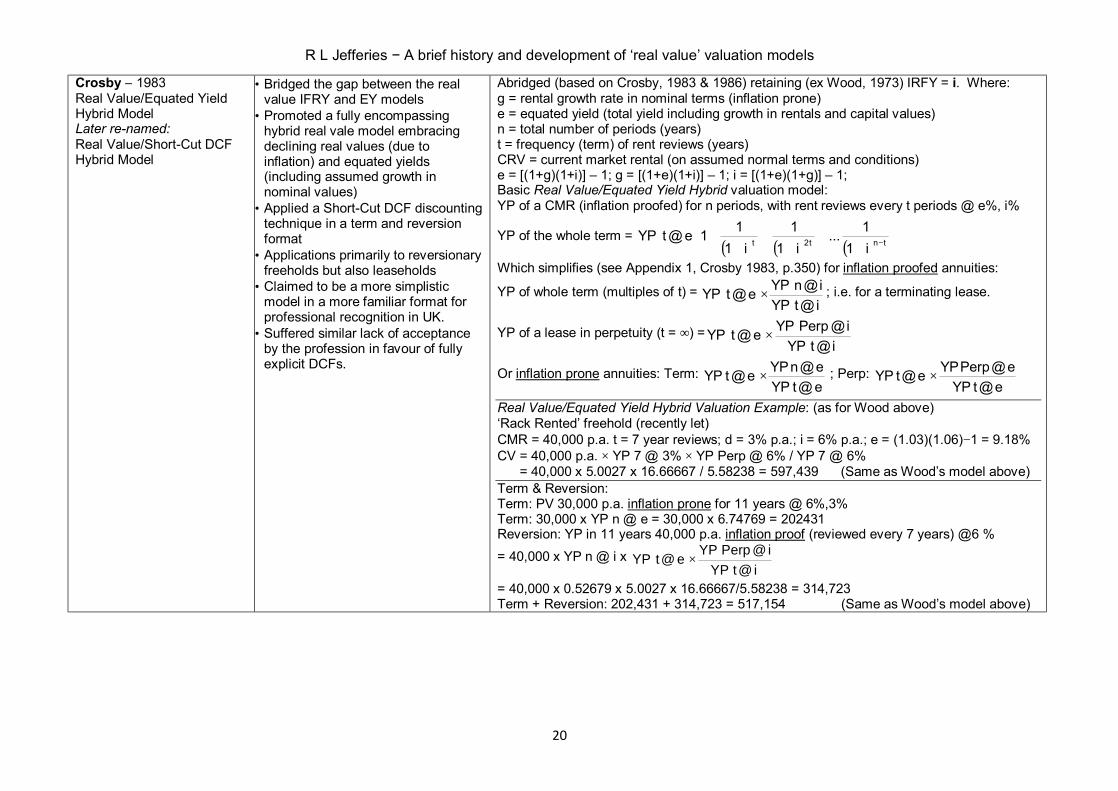
Crosby – 1983 Real Value/Equated Yield Hybrid Model Later re-named: Real Value/Short-Cut DCF Hybrid Model

• Bridged the gap between the real value IFRY and EY models

• Promoted a fully encompassing hybrid real vale model embracing declining real values (due to inflation) and equated yields (including assumed growth in nominal values)

• Applied a Short-Cut DCF discounting technique in a term and reversion format

• Applications primarily to reversionary freeholds but also leaseholds

• Claimed to be a more simplistic model in a more familiar format for professional recognition in UK.

• Suffered similar lack of acceptance by the profession in favour of fully explicit DCFs.

Abridged (based on Crosby, 1983 & 1986) retaining (ex Wood, 1973) IRFY = i. Where: g = rental growth rate in nominal terms (inflation prone) e = equated yield (total yield including growth in rentals and capital values) n = total number of periods (years) t = frequency (term) of rent reviews (years) CRV = current market rental (on assumed normal terms and conditions) e = [(1+g)(1+i)] – 1; g = [(1+e)(1+i)] – 1; i = [(1+e)(1+g)] – 1; Basic Real Value/Equated Yield Hybrid valuation model: YP of a CMR (inflation proofed) for n periods, with rent reviews every t periods @ e%, i%

YP of the whole term = ( ) ( ) ( )

++

++

++

−tnt2t i11...

i11

i111e@tYP

Which simplifies (see Appendix 1, Crosby 1983, p.350) for inflation proofed annuities:

YP of whole term (multiples of t) =i@tYPi@nYPe@tYP × ; i.e. for a terminating lease.

YP of a lease in perpetuity (t = ∞) =i@tYP

i@PerpYPe@tYP ×

Or inflation prone annuities: Term: e@tYPe@nYPe@tYP × ; Perp:

e@tYPe@PerpYPe@tYP ×

Real Value/Equated Yield Hybrid Valuation Example: (as for Wood above) ‘Rack Rented’ freehold (recently let) CMR = 40,000 p.a. t = 7 year reviews; d = 3% p.a.; i = 6% p.a.; e = (1.03)(1.06)−1 = 9.18% CV = 40,000 p.a. × YP 7 @ 3% × YP Perp @ 6% / YP 7 @ 6% = 40,000 x 5.0027 x 16.66667 / 5.58238 = 597,439 (Same as Wood’s model above) Term & Reversion: Term: PV 30,000 p.a. inflation prone for 11 years @ 6%,3% Term: 30,000 x YP n @ e = 30,000 x 6.74769 = 202431 Reversion: YP in 11 years 40,000 p.a. inflation proof (reviewed every 7 years) @6 %

= 40,000 x YP n @ i x i@tYP

i@PerpYPe@tYP ×

= 40,000 x 0.52679 x 5.0027 x 16.66667/5.58238 = 314,723 Term + Reversion: 202,431 + 314,723 = 517,154 (Same as Wood’s model above)


21

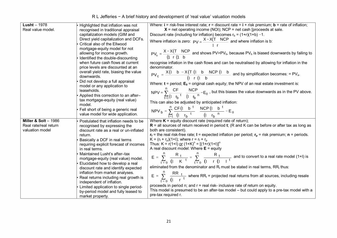
Lusht – 1978 Real value model.

• Highlighted that inflation was not recognised in traditional appraisal capitalization models (GIM and Direct yield capitalization and DCFs.

• Critical also of the Ellwood mortgage-equity model for not allowing for income growth.

• Identified the double-discounting when future cash flows at current price levels are discounted at an overall yield rate, biasing the value downwards.

• Did not develop a full appraisal model or any application to leaseholds.

• Applied this correction to an after–tax mortgage-equity (real value) model.

• Fell short of being a generic real value model for wide application.

Where: i = risk-free interest rate; r = discount rate = i + risk premium; b = rate of inflation; X = net operating income (NOI); NCP = net cash [proceeds at sale. Discount rate (including for inflation) becomes rb = (1+r)(1+b) −1. Where inflation is zero: ( )

rNCPTXXPV

++−

=1

and where inflation is b:

( )( )( )b1r1

NCPTXXPVb +++−

= and shows PV>PVb, because PVb is biased downwards by failing to

recognise inflation in the cash flows and can be neutralised by allowing for inflation in the denominator.

( ) ( )( ) ( )( )( )br

bNCPbTXbXPVc +++++−+

=11

111 and by simplification becomes: = PVa.

Where: t = period; E0 = original cash equity; the NPV of an real estate investment is:

( ) ( ) 01 11

Er

NCPr

CFNPV nb

n

tt

b−

++

+= ∑

=

, but this biases the value downwards as in the PV above.

This can also be adjusted by anticipated inflation: ( )

( )( )

( ) 01 1

1

1

1 Er

bNCPr

bCFNPV nb

tn

tt

b

tb −

+

++

+

+= ∑

=

Miller & Solt – 1986 Real rate/real return valuation model

• Postulated that inflation needs to be recognised by expressing the discount rate as a real or un-inflated return.

• Basically a DCF in real terms requiring explicit forecast of incomes in real terms.

• Maintained Lusht’s after–tax mortgage-equity (real value) model.

• Elucidated how to develop a real discount rate and identify expected inflation from market analyses.

• Real returns including real growth is independent of inflation.

• Limited application to single period-by-period model and fully leased to market property.

Where K = equity discount rate (required rate of return); R = all sources of return received in period t; (R and K can be before or after tax as long as both are consistent). rf = the real risk-free rate; I = expected inflation per period; rp = risk premium; n = periods. K = (rf + rp)(1+I); where r = rf + rp Thus: K = r(1+I) or (1+K)n = [(1+r)(1+I)]n

A real discount model: Where E = equity

( ) ( )( )∑∑== ++

=+

=n

tt

tn

tt

tIr

RK

RE00 111

and to convert to a real rate model (1+I) is

eliminated from the denominator and Rt must be stated in real terms, RRt thus:

( )∑= +

=n

tt

tr

RRE0 1

where RRt = projected real returns from all sources, including resale

proceeds in period n; and r = real risk- inclusive rate of return on equity. This model is presumed to be an after-tax model – but could apply to a pre-tax model with a pre-tax required r.


22

Kemplerer – 1979 Real market interest rate, inflation excluded model

• Presented two models in real terms borrowed from forestry valuation.

• Applied to terminating incomes. • Distinguished geometric growth due

to inflation separately from real growth in income.

• Applied a ‘real interest rate’, inflation excluded’.

• Did suggest a perpetual growth formula.

• Did not develop a full real estate appraisal model – only annually in arrears, annual growth, and full-equity only.

Where: i = real interest rate (inflation excluded); g = real annual rate of growth or decline; id = downward adjusted interest rate for capitalizing rising payments with fixed formula; iu = upward adjusted interest rate for capitalizing declining payments with fixed formula; V0 = present value in year 0; n = number of payments (or No years for annual series); y = number of periods between payments (y = 1 for annual series); p = amount that the first payment would be if it occurred in period 0 (since at end of first period =p(1+g)y for rising payments). Interest rate adjustment to use standard discounting formulas or compound interest tables:

For rising payments ( )( )

gi,ggi

g︶iid ≠

+−

=−++

=1

111 ;

For declining payments: by factor of 1/(1+g): ( )( ) iggiiiiu ++=−++= 111 Real cash flows− fixed:

( )( )n

n

iiipV+

−+=

111

0, If g = i for terminable series V0 = np, when i = g; for perpetual series, g < i.

Real cash flows− Rising at g% annually: substitute id in above formula. Real cash flows− Declining at g% annually: substitute iu in above formula.

Blackadar – 1980-89 Dynamic Capitalization model

• Most comprehensive of the USA models but in actuarial formulae and IAN notations

• Complex formulations with difficulty in appraiser understanding and skill acquisition required.

• Identifies currency inflation separate from real value depreciation or appreciation (growth).

• Did not provide a generic model in a capitalisation model format or formula but presented as a ‘varying annuity function’ as a Effective Gross Income Multiplier (GIM).

• This function is applied to the effective gross income (EGI) – requiring a preliminary income adjustment as vacancy not allowed in the model calculations).

• The IAN symbols used are a shorthand way of giving the frequencies with which the moneys are paid and timing of payments, i.e. in advance or arrears.

Simplified – based on Blackadar,1989 – Where: IAN symbols & notations used: i(12), d, d(1/5) refer to a capital asset of unit value (a multiplier) with rent at various frequencies; i = nominal rate of interest (represent payments in arrears); d indicates a nominal rate of discount (payments in advance); the “upper” (in parentheses) indicate the frequency i.e. No payments p.a. i.e. i(12) rent paid monthly in arrears, d(1/5) rent paid five yearly in advance; whilst simple exponents i.e. v20 means “raised to a power”. (va) refers to the PV of a varying annuity; nominal rates of interest i or nominal rate of discount d are rent equivalents paid at p; q or r = frequency of payments ; YIELD = real required rate of return. n = No of periods for which the payments continue Adjustments to yield are: CURRENCY = (+ve) for currency erosion due to inflation; LSR = lease stipulated recovery (i.e. rent increase linked to CPI or % thereof); ASSET = (+ve) for asset depreciation – a loss in the ability to command rent (or –ve) for appreciation in real terms; 1 is the value of a unit asset invested at n = 0. For a lease in perpetuity or perpetually renewable the term is ⌉ = ∞⌉. The dynamic capitalization general ‘varying annuity function’ model – called an ‘equation of value’ that produces a GIM (multiplier) applied to the EGI from a real estate investment: ( ) ⌉( )( )( ) = ( ) ( ) ( )

( ) ( ) (“×” sign between ratios is omitted)

Asset value = EGI × ( ) ⌉( )( )( ) = EGI × multipliers for: leases × LSR × exit value and/or extraordinary expenses On the right-hand side of the equation the first two varying annuity functions are called


23

• Uses a variant of Short-Cut DCF in real terms.

• Allows adjustment for market cycle variations, modifications called ‘special effects’. These are made in the ‘equation of value’ that allow for lease-up and extraordinary expenses at lease turnovers, including rent abatements.

• Also adapts to adjust for market disequilibrium for growth rates that change over defined periods as ‘split-rate spline’ equations.

• Adapts to mortgage leveraging allowing for debt service and using a real yield on equity and can be applied to an after-tax model.

• Basic model assumes the current rent is newly let at a market rent in an on-going lease in perpetuity, or in a reversion.

• A terminating lease requires re-formatting (adjustment) to the equation of value.

• Re-formatting is also required for typical property subject to a lease on contract rent and/or different terms from current market terms. This requires use of ‘split-rate spline’ equations of value, in a ‘term + reversion’ format).

• Lost on the profession of appraisers due to complexity, ‘actuarial language’ and expressions.

• Also laborious method to calculate manually – but could (now) be adapted into a spreadsheet model. (as used by this author to do the calculations in the example opposite)

synchronizing functions that adjust the annuity function for the dynamics of the cash flows. ( ) ( ) The ( ) nominator (being an annuity multiplier of rent earned) is adjusted by the

denominator ( ) for real yield and currency erosion (see Blackadar, 1986) ( ) ( ) The ( ) nominator (being the LSR annuity multiplier) is adjusted by the by the

denominator ( )for real yield and LSR as a (–ve) as offsetting currency erosion. ( ) The denominator ( ) (being the exit capitalization rate for the reversionary asset

value for real yield, currency erosion/(-ve) for inflationary growth and (+ve) asset depreciation recovery.

Similar functions can be added for other recurring income or expenditure such as unrecovered OPEX (see Blackadar, 1984). Simple Dynamic capitalization example: ex Wood and Crosby example (above) Contract Rent (RC) = 30,000 p.a.; let 3 years ago on 14 year lease (fixed for 11 years to run) Current Market Rental (RM)= 40,000 p.a. with 7 year rent reviews CURRENCY = 3% p.a. nominal inflation rate, annually in arrears = growth in real terms. i = 6.0% p.a. effective real nominal interest rate, annually in arrears d = 5.6604% p.a. effective real nominal discount rate, annually in advance (= 6.0%/1.06) ASSET depreciation = 0%; and LSR = 0% – as do not apply in this example; Vn = the PV of a sum discounted n periods @ i. = (1 + ) 1−Vn = the total discounted PV of a sum discounted n periods @ i. = 1 − (1 + ) Asset = value of the asset (property) at period 0. The equation of value ( ) ⌉( )( )( ) needs modification, ‘split-rate spline’ equations for the contract term to run element C at the end of the fixed contract rental to run; and separately for the deferred reversionary market rental review basis M (then assumed) in perpetuity. The first synchronizing function remains and is separated to apply to the contract rent RC The second synchronizing function, the adjustment for LSR, is omitted as not applicable. The third function is applied separately as a ‘split-rate spline’ of Vn to the contract rent (RC) and 1-Vn to the current market rent RM, in which the currency inflation is offset (assuming rental increases in nominal terms to offset inflation – i.e. static in real terms − thus: ( ) ⌉( )( )( ) = ⎣⎢⎢

⎡ ( ) ( ) ( ) ⎦⎥⎥

⎤ + ( ) ⌉( )( )( ) = ⎣⎢⎢⎡ ( ) ( ) ( )

( ) ⎦⎥⎥⎤


24

[The author has struggled to interpret this model and do the resulting calculation in the next column. It is intuitively illogical − the capitalization rate for the contract rent RC 0.43019 appears low compared to the market rent RC 0.47849 to reflect the longer delay to achieving growth. Thus the term is over-valued at 241,047 c/- to 202,431 and the reversion under-valued at 248,798 c/- 314,723 in the other real value model examples. Perhaps a reader can suggest the correct figures!]

= 30,000 0.0566040.0900000.5267880.043019 + 40,000 0.0566040.0900000.4732120.047849

Where (pC), (qC ), (pM), (qM ) = 1 (rent paid annually in arrears) (rC ) = (1/11), n = 11 fixed 11 year Contract rent term to run; (rM ) = (1/7) Market rent for 7 year reviews terms

= R ⎣⎢⎢⎡ ( ) ( )

( / ) ⎦⎥⎥⎤ + R ⎣⎢⎢

⎡ ( ) ( ) ( / ) ⎦⎥⎥

⎤

(30,000 × 0.628933 × 12.245473) + (40,000 × 0.628933 × 9.88969) 231,047+ 248,798 = 479,845 Differs significantly from Wood’s and Crosby’s example (above)

Jefferies 1997 − Generic Real Value

• Simple basic real value concept and generic model

• Basically in a Short-Cut DCF and Term & Reversion format.

• Distinguishes between currency inflation and real growth effects .

• All cash flows expressed in current real values.

• Avoids double-discounting to execute a real terms DCF.

• User-Friendly spreadsheet model application

• Adaptable to multi-tenanted properties

• International application • Extended to variation of leasehold

valuations. • A generic real value model similarly

readily adapts to allow for: § A vacancy or rent-up period with

re-leasing or upgrading costs on expiry of the current lease

§ Where vacant space occurs, the existing rental will either be nil or the lessor will be carrying un-recovered operating expenses

§ Different types of terminal, residual or reversionary values

§ A negative value, e.g. an on-

Ve is the “Effective investment value” at date of valuation, subject to an existing lease. ⇐ indicates that investment value is derived from cash flows and is not reversible. PV is defined as “present value”; where: Yo is the overall investment yield; and f is the payment frequency per year. A conventional DCF valuation model re-expressed in real terms where I is the expected inflation rate is: Ve ⇐ PV of future periodic cash flows + PV of reversionary or terminal value [Each cash flow is first discounted at the expected inflation rate, I ] i.e., discounted @ i annually (p.a.); or i per period (p.p.) where: 1I1i f −+= Which produces cash flows in real terms: Ve ⇐ PV of future periodic real cash flows + PV of future real reversionary value i.e., discounted at a real rate of return ( ) ( )[ ] 111 −++= IYY or , or p.p. @ 11 −+= fr Yy

A real value generic DCF valuation model, where Go is the growth rate is: Ve ⇐ PV of future periodic cash flows Discounted at a nominal or monetary rate of return i.e. investment yield rate, Yo +PV of deferred current real reversionary or terminal value Discounted at a net (of growth) investment yield rate, ( ) ( )[ ] 1G1Y1Y oon −++=

i.e., discounted @ Yn annually (p.a.); or p.p. where: 1Y1y fnn −+=

C = Contractual fixed cash flows until the next rental review as a regular annuity. t = periods to run until next review Ca = PV of discounted at a required overall investment yield Yo Vr = the current real reversionary or terminating value subject to the existing lease. Vr = the current contract review rental Mc capitalised at a contract review rental capitalisation rate Ec, i.e. Vr = Mc/Ec. The PV of Vr is discounted at the net (of growth) investment yield Yn.p.a. [This is because the current value is in real terms, not a forecast as at the review date, and only requires discounting for delay and risk.]


25

going environmental, remedial or demolition cost

(See Appendix A)

APPLICATION OF REAL VALUE LEASEHOLD MODEL An adaptation of the generic real value model and the ExcelTM template model has been developed for the valuation of leasehold interests. The lessor’s interest model requires very little alteration to the generic model as the principles and methodology is basically unchanged, requiring only some re-wording. The lessee’s model is similar but the lessee’s benefit rental is discounted at the lessee’s required return Ylo and any rights of renewal or occupational value in real terms discounted at the lessee’s net of growth required return Yln The formulation of this model and examples of its use is detailed in Jefferies, 1997b.

Ec may be derived from the market by analysis of sales of comparable properties with (or adjusted to) the same contract reviews and date. Ec equates to an initial return rate as at the rental review date reflecting the lease terms. Ec can be calculated given an investment yield, growth rate and lease review terms, as in shown in Jefferies, 1997a - APPENDIX A. The simplified generic real value model subject to an existing lease is: Ve ⇐ PV of future periodic cash flows (to next review) +PV of deferred current real reversionary value (subject to lease) = Ca + Vr(1+Yn)–t The generic real value model assumes a renewable lease with a right of renewal in perpetuity or re-let on expiry at the same terms and conditions as the existing lease. Mm = current open market rental and capitalising it at an open market capitalisation rate Em, gives the current real open market value i.e. Vm = Mm/Em. The generic real market value model is therefore re-expressed as follows: Ve ⇐ PV of future periodic cash flows +PV of deferred current real market value (unencumbered by lease) = Ca + Vm(1+Yn)–t The generic real value model readily adapts to a terminating investment, i.e., assuming the investment stops at the end of the lease without any residual value. The assumed reversionary value is “slicing off” and deferred to the lease expiry or termination date where X = no periods to expiry or termination: Ve ⇐ PV of future periodic cash flows +PV of remaining review terms to expiry (subject to lease) =Ca + Vr[(1+Yn)–t – (1+Yn)–X] Generic Real Value Valuation Example: (as for Wood and Crosby’s model above) C = 3,000 p.a.; let 3 years ago on 14 year lease (11 years to run) ; Yo = 9.18% Mm = 4,000 p.a. with 7 year reviews; d Go = 3% p.a. and Yn = 6% p.a. Ve ⇐ PV of future periodic cash flows +PV of deferred current real market value (unencumbered by lease) = Ca + Vm(1+Yn)–t Ca = PV of the contract rental to expiry date = PV @ Required overall investment yield Yo as % p.a., for No rental periods to run to the next review of actual contract rental paid per payment period. = PV 30000 p.a. @ 9.18% p.a. for 11 years = 30,000 x 6.74769 = 202,431 Vm(1+Yn)–t = PV of real reversionary value at expiry date =PV @ Yn as % p.a., of current market value assuming market rental capitalised at market rental capitalisation rate Em, as at the expiry of existing lease term in t rental periods to run. PV of 40000 p.a., capitalised @ (0.0918-0.0918((1.03)7-1)/((1.0918)7-1))=6.69524% p.a. =597,438 discounted for 11 years @ 6.0% p.a. (0.52679) = 314,723 Ca + Vm(1+Yn)–t = 202,431 + 314,723 = 517,154 (same as Wood’s and Crosby’s above)

26

References:

Baum, A. and Crosby, N. (2008) (3rd edn) Property Investment Appraisal Oxford, Blackwell Publishing.

Baum, A., Mackmin, D. and Nunnington, N. (1997) (4th edn) The Income Approach to Property Valuation London: International Thomson Business Press.

Blackadar, C. G. (1984) “Dynamic Capitalization: An Income Approach in Real Dollars at Real Interest” The Appraisal Journal October 565-594.

Blackadar, C. G. (1986) “Dynamic Capitalization: An Income Approach in Real Dollars at Real Interest, Part 2: Making it Work for You” The Appraisal Journal July 325-355.

Blackadar, C. G. (1989) “Dynamic Capitalization: An Income Approach in Real Dollars at Real Interest, Part 3: The Dynamics of Expectations” The Appraisal Journal July 338-371.

Bradley, D. M. (1989) “The Capitalization Rate, the Discount Rate, and Inflation” The Appraisal Journal April 237-243.

Brown R. J. and Johnson, D. A. (1980) “Inflation, Valuation, and the Discount Rate” Appraisal Journal, October, 549-555.

Brown, G. R. (1991) Property Investment and the Capital Markets London: E & FN Spon Clark, R. E. (1978) “Equated Yield Analysis” The Estatesman, April. Crosby, N. (1982) “The investment method of valuation: A real value approach” RICS Junior

Organisation, Ryde Memorial Prizewinning Paper. (Reproduced in Crosby (1985) Vol. 2, Appendix II, 846-862)

Crosby, N. (1983) “The investment method of valuation: A real value approach” Journal of Valuation 1(4) 1983, 341-350, 2, 48-59.

Crosby, N. (1984) “Investment valuation techniques: The shape of things to come” The Valuer (UK) 53(7), 196-197. [don’t have part II ??]

Crosby, N. (1985) "The application of equated yield and real value approaches to the market valuation of commercial property. Unpublished thesis (Ph.D.) - University of Reading, Department of Land Management and Development.

Crosby, N. (1986a) “Real value, rational model, D.C.F. : A reply” Journal of Valuation 4, 16-20. Crosby, N. (1986b) “The application of equated yield and real value approaches to market

valuation: 1 − The logic of techniques and analysis of comparables”; II – “…Equivalent yield or equated yield approaches?” Journal of Valuation 4, 158-169; 261-274.

Davidson, A. W. (2002, 12th ed) Parry’s Valuation & Investment Tables, London: The Estates Gazette.

French, N. (1996) “Investment valuation. Developments from the Mallinson Report” Journal of Property Valuation and Investment 14(5), 48-58.

Gibbons, J. E. (1986) “Comments on: Finance Theory and Real Estate Valuation” in Kinnard, W. N. Jnr. (ed) 1984 Real Estate Valuation Colloquium. A redefinition of Real Estate Appraisal Precepts and Processes. A Lincoln Institute of Land Policy Book, Boston MA: Oesgeschlager, Gunn & Hain., 90-95.

Goolsby, W. C. (1983) “How Inflation-induced Interest Rates Affect Property Value” The Appraisal Journal, April, 234-239.

Greaves, M. J. (1972) “Discounted cash flow techniques and current methods of income valuation” Estates Gazette 223, 2147-2155 and 233: 2239-2245.

Harris, J. C. (1983) “Applying Ellwood in an Era of Persistent Inflation” The Real Estate Appraiser and Analyst, Spring, 15-17.

Jefferies, R. L. (1978) (1st edn) Urban Valuation in New Zealand – Vol. I Wellington, NZ: The New Zealand Institute of Valuers.

Jefferies, R. L. (1990) (Ed.) Urban Valuation in New Zealand – Vol. II Wellington, NZ: The New Zealand Institute of Valuers.

Jefferies, R. L. (1991) (2nd edn) Urban Valuation in New Zealand – Vol. I Wellington, NZ: The New Zealand Institute of Valuers.


27

Jefferies, R. L. (1995a) DCF Valuation Techniques & Spreadsheet Applications — A CPD Monograph Wellington, NZ: New Zealand Institute of Valuers.

Jefferies, R. L. (1995b) “DCF valuation calculations and presentation in valuation reports” in The Cutting Edge 1995 Property Research Conference of the Royal Institution of Chartered Surveyors, University of Aberdeen, Scotland, 1-2 September, Proceedings Vol 2: 89-112

Jefferies, R. L. (1995c) “Discounted Cash Flow Valuations — Pitfalls, Standards & Solutions” Proceedings of the First International Real Estate Society Conference, Stockholm, Sweden, June 28 - July 1.Jefferies, R. L. (1997a) “A generic ‘real value’ valuation model” Paper presented to the European Real Estate Society Conference, European Business School, Berlin, Germany, June, 1997.

Jefferies, R. L. (1997b) “A ‘real value’ lessor’s and lessee’s interest valuation model” Paper presented to the European Real Estate Society Conference, European Business School, Berlin, Germany, June, 1997.

Klemperer, W. D. (1979) “A simplified Technique for Capitalising Geometrically Changing Cash Flows” The Real Estate Appraiser and Analyst March-April 11-13.

Korpacz P.F. and Roth, M. I. (1983) “Changing Emphasis in Appraisal Techniques: The Transition to Discounted Cash Flow” The Appraisal Journal, January, 21-24; April 315-316.

Kuehnle, W. R. (1979) “Real estate values and inflation: The value of real estate versus the value of money” Real Estate Issues, 4, No.1, 17-19.

Lusht, K. M. (1979) “Inflation and Real Estate Investment Value” The Real Estate Appraiser and Analyst Nov-Dec 23-29.

Lusht, K. M. (1979) “The Behaviour of Appraisers in Valuing Income Property: A Status Report” The Real Estate Appraiser and Analyst July-August 49-59.

Lusht, K. M. (2000) Real Estate Valuation- Principles and Practice New York : McGraw-Hill Primis Custom Publishing.

Lusht, K. M. and Zerbst, R. H. (1980) “Valuing Income Property in an Inflationary Environment” The Real Estate Appraiser and Analyst Jul-Aug 11-17

Marshall, P. (1976) “Equated yield analysis A valuation method of the future” Estates Gazette 239, 493-497.

Marshall, P. (1979) (2nd edn) Donaldsons Investment Tables London: Donaldsons. Mason, R. C. (1983) “Present Worth in Present Dollars” The Appraisal Journal July 415-421. Miller N.G.and Solt M.E. (1986) “Using a real discount rate model is better than predicting inflation”

The Appraisal Journal, April, 188-197. Rhodes, F. G. (1981) “Inflation Discounting: How Appraisers can Deal with Inflation” The Appraisal

Journal April 234-247. RICS, (1994) The Mallinson Report − The President’s Working Party on Commercial Property

Valuations, London: Royal Institution of Chartered Surveyors. RICS, (1997) Commercial Investment Property Valuation Methods − An Information Paper, London,

Royal Institution Of Chartered Surveyors. Ring, A. A. (1970) The Valuation of Real Estate, Englewood Cliffs, NJ, Prentice-Hall. Ryan, J. P. (1992) “Real Rates of Returns: Does Real Estate Make Sense” Real Estate Issues

Fall/Winter, 17-20. Sayce, S. Smith, J, Cooper, R. and Venmore-Rowland, P. (2006) Real Estate Appraisal. From Value

to Worth, Oxford, Blackwell Publishing. Scarrett, D. (2008) 2nd Edn Property Valuation – the five methods, Routledge, London. Sevelka, T. (2004) “Where the overall cap rate meets the discount rate” Appraisal Journal, Spring,

135-146. Slay, K. D. (1990) “The Capitalisation Rate, the Discount Rate, and Projected Growth in Value”

The Appraisal Journal July 324-327. Sykes, S. G. (1980) “Aspects of Property Capital Growth and Its Interpretation” The Investment

Analyst 56, 21-30. Sykes, S. G. (1981) “Property valuation: a rational model” The Investment Analyst 61, 20-26.


28

Sykes, S. G. (1983) “Valuation models: action or reaction” Estates Gazette 267, 1108 - 1112. Sykes, S. G. and McIntosh A. (1983) “Towards a Standard Property Income Valuation Model:

Rationalisation or Stagnation" Journal of Valuation Vol 1, 121-?. Sykes, S. G. and Young, M. S. (1981) “A Differential Approach to Income Property Valuation: A new

Measurement Technique” The Appraisal Journal April, 214-233. Trott, A. J. (1980) (ed) RICS Property Valuation Methods: Interim Report, London: Polytechnic of the

South Bank. Trott, A. J. (1986) (ed) Property Valuation Methods London: Royal Institution Of Chartered Surveyors

& Polytechnic of the South Bank. Wendt, P. F. (1977) “Inflation and the Real Estate Investor” The Appraisal Journal July 343-355. Wood, E (1972) "Property Investment – a real value approach" unpublished PhD Thesis,

Department of Valuation Studies and Land management and Development, Reading University, United Kingdom.

Wood, E. (1967) "Valuation techniques for the seventies" Chartered Surveyor, October, 196-197. Wood, E. (1973) “Positive valuations – A real value approach to property investment” Estates

Gazette Vol 226: I - 923-925, II - 1115-1116, III - 1311-1313. Wood, E. (1986) "Positive Valuation Methods" Journal of Valuation 4, (1) 7-15 & 4, (2) 170-184. Wyatt, P. (2007) Property Valuation in an economic context Oxford, Blackwell Publishing Young, M. S. (1980) “Inflation, Valuation, and the Petersburg Paradox” The Appraisal Journal

January 85-94.

APPENDIX A A terminating lease real value model similarly readily adapts to allow for: • A vacancy period with re-leasing or upgrading costs on expiry of the current lease: Where U = vacancy period; H = current real re-leasing/upgrading costs) Ve ⇐ PV of future periodic cash flows +PV of remaining review terms to expiry (subject to lease) ± PV of real terminal value = Ca + Vr[(1+Yn)–t – (1+Yn)–X] + (Vm – H)(1+Yn)–(X+U) • Where vacant space occurs, the existing rental will either be nil or the lessor will be carrying un-recovered

operating expenses, i.e. Ca will be nil or negative (–ve). • Where operating expenses are defined as O. • The present value of these are discounted at Yn over the forecast current vacancy period Uo to lease-up

as Oa. The model re- expressed replacing Ca with Oa, and t with Uo: Where Uo = initial vacancy period; H = current real re-leasing/upgrading costs) Ve ⇐ PV of operating expenses over vacancy period ±PV of real leased-up value = –Oa + (Vm – H)(1+Yn)–Uo The generic real value model is also readily adaptable to allow for a terminating lease with different types of terminal, residual or reversionary values, for example: • An alternative use, e.g. redevelopment of the existing building or site; Where VX = current real terminal value. Ve⇐ PV of future periodic cash flows +PV of remaining review terms to expiry (subject to lease) ±PV of real terminal value = Ca + Vr[(1+Yn)–t – (1+Yn)–X] + VX(1+Yn)–X • A negative value, e.g. an on-going environmental, remedial or demolition cost. • As the latter values are in current or real values they will only increase by inflation over the remaining

period to lease expiry and should be discounted at a real discount rate Yr Where VX = current real terminal value; D = current real residual costs.

Ve⇐ PV of future periodic cash flows +PV of remaining review terms to expiry (subject to lease) ±PV of real terminal value = Ca + Vr[(1+Yn)–t – (1+Yn)–X] + VX(1+Yn)–X – D(1+Yr)–X


29

APPENDIX B

REAL VALUE LESSOR'S INTEREST INVESTMENT VALUATION MODEL ©R L Jefferies 1997

Enter inputs in RED bordered cellsValuation (or Sale) Date (dd/mm/yyyy): 01/Jan/2009 Sale price (if known, or applicable)

Lease Last rental review date (dd/mm/yyyy): 01/Jan/2006 Details: Termination or expiry date: Leave blank if renewable 01/Jan/2020

Rental runs to expiry date = 01/Jan/2020Contract rental (per annum): 30,000.00 p.a. Contract rental review term (years): 15.00 years No. rental payments per year 1 times per year Rental payment basis: Enter '1' if BOP or '0' if EOP 0

Inputs: Required overall investment yield: Yo as % p.a. 9.18% p.a.Forecast overall growth rate: Go as % p.a. 3.00% p.a.Expected inflation rate: I as % p.a. (optional)Normal open market rental review term (years) 7.00 years Normal open market rental p.a. (on market review terms) 40,000.00 p.a.

Calcs: Net (of growth) yield: Yn = (1+Yo)/(1+Go) –1 as % p.a. 6.00% p.a.Current contract review rental (adj. to review terms) 43,650.91 p.a.

If Re- Forecast vacancy period ( 0 if no vacancy or +ve number) 0.00 periods leasing: Forecast re-leasing costs (as -ve) in current valuesIF Terminating: Enter terminal value (costs as -ve) in current values

Valuation: (based on effective per period rental payment, discount and capitalisation rates)

PV of the contract rental to expiry date = 202,431

+ PV of real reversionary value at expiry date = 314,723

+ PV of real forecast re-leasing costs at expiry Model calculates PV if Re-Leasing

+ PV of real forecast terminal value or costs Model calculates PV if terminating

= TOTAL PRESENT VALUE: VE 517,154

Solve for Rental Growth given

lessor's yield & sale price

Solve for Lessor's Yield given rental

growth & sale

Clear input details & inputs

REAL VALUE LESSEE'S INTEREST INVESTMENT VALUATION MODEL ©R L Jefferies 1997

Enter inputs in RED bordered cellsValuation (or Sale) Date (dd/mm/yyyy): 01/Jan/2009 Sale price (if known, or applicable)

GROUND or HEAD-LEASE DATA :(Entered in Lessor's Sheet)Lease Last rental review date (dd/mm/yyyy): 01/Jan/2006Details: Termination or expiry date: 01/Jan/2020

Rental runs to expiry date = 01/Jan/2020Contract rental (per annum): 30,000.00 p.a. Contract rental review term (years): 15.00 years No. rental payments per year 1 times per year Rental payment basis: Enter '1' if BOP or '0' if EOP 0

Inputs: LESSEE'S overall investment yield: Ylo as % p.a. 11.18% p.a.Forecast overall growth rate: Go as % p.a. 3.00% p.a.Expected inflation rate: I as % p.a. (optional) 0.00% p.a.Affordable ground/head-lease rental: Ma p.a. 45,000.00 p.a.

Calcs: Lessee's net (of growth) yield: Yln = (1+Ylo)/(1+Go) –1 as % p.a. 7.94% p.a.Current ground/head-lease review rental 43,650.91 p.a.

IF Terminating: Current Lessee's terminal value (or costs as -ve): Tc

SUB-LEASE DATA :(ENTER IF Applicable)Building sub-lease contract rental(s): Bc = Building sub-lease current review rental(s): Bb = Building sub-lease rental periods to run to next reviews(s) tb = Building sub-lease rental review terms (years): pb = Building sub-lease payment frequency - times per year : fb = Building sub-lease rental forecast growth rate: Gb = Building sub-lease rental basis: Enter '1' if BOP or '0' if EOP

LESSEE'S INTEREST VALUATION: (on effective p.p. rental payment, discount and capitalisation rates)PV of the rental benefit to expiry date :Ba = 92,351

+ PV of real Rights of Renewal value at expiry date: RoR= 6,075PV of real added occupational value or cost TO LESSEE: Occ = No Added Occupational Use Value

+ PV of real lessee's terminalvalue or costs -ve PV Tc = Shows PV if Terminating & Tc Entered

= TOTAL PRESENT VALUE of Lessee's Interest: VL 98,426

Solve for Building Growth given Lessee's

yield & sale price

Solve for Lessee's Yield given building rental growth & sale price

Clear input details & inputs


30

Footnotes: i For example, a 20 year terminating lease allowing for a projection to termination with monthly rental

payments would require 240 (20x12) spreadsheet columns (or rows) to properly use the NPV or IRR formulae. For this reason DCFs are frequently calculated annually in arrears (or end of period - EOP) even though rentals are actually paid more frequently and usually in advance (or beginning of period - BOP).

ii In concept the model, as does the traditional “equated yield” model and direct capitalisation methodologies, assumes the lease is renewed in perpetuity or where by statute or contract some leases are “perpetually renewable” in some countries - ie some ground leases in The Netherlands, Hawaii, New Zealand

iii In the model, a message will appear, for example, if anything other than a “0” or “1” is inputted into the rental payment basis cell to indicate whether payments are BOP or EOP , ie “Enter ‘0’ or ‘1’ ”; and if a figure is entered in both the re-leasing input cells and the terminating value/cost input cells then a message “Incompatible with terminating assumption” and vice versa message “Incompatible with re-leasing assumption messages appear.

a brief history and development of ‘real value’ valuation

Documents