a branch-and-cut-and-price algorithm for the multi-trip separate … · 2018. 11. 2. · a...

A Branch-and-Cut-and-Price Algorithm for the Multi-Trip Separate Pickup and Delivery Problem with Time Windows at Customers and Facilities Andrea Bettinelli Valentina Cacchiani Teodor Gabriel Crainic Daniele Vigo November 2018

CIRRELT-2018-45

A Branch-and-Cut-and-Price Algorithm for the Multi-Trip Separate Pickup and Delivery Problem with Time Windows

at Customers and Facilities Andrea Bettinelli1, Valentina Chacchiani2, Teodor Gabriel Crainic3,*, Daniele Vigo2

1 OPTIT Srl, Viale Amendola 56/D, 40026 Imola (BO), Italy 2 DEI, University of Bologna, Viale del Risorgimento 2, 40136 Bologna, Italy 3 Interuniversity Research Centre on Enterprise Networks, Logistics and Transportation (CIRRELT)

and Department of Management and Technology, Université du Québec à Montréal, P.O. Box 8888, Station Centre-Ville, Montréal, Canada H3C 3P8

Abstract. We study the Multi-trip Separate Pickup and Delivery Problem with Time Windows at Customers and Facilities (MT-PDTWCF), arising in the context of two-tiered city logistics systems. The first tier refers to the transportation between the city distribution centers, in the outskirts of the city, and intermediate facilities, while the second tier refers to the transportation of goods between the intermediate facilities and the (pickup and delivery) customers. We focus on the second tier, and consider that customers and facilities have time windows in which they can be visited. Waiting is possible at waiting stations for free or at customers and facilities at a given cost or penalty. Therefore, it is relevant to synchronize the arrivals of vehicles at facilities and customers with the corresponding time windows. The MT-PDTWCF calls for determining minimum (fixed, routing and waiting) cost multi-trip routes, for a given fleet of vehicles, to service separately pickup and delivery customers, while taking into account vehicle capacity and time windows both at customers and facilities. This problem, recently introduced in the literature, generalizes several variants of the Vehicle Routing Problem. We propose the first exact algorithm for MT-PDTWCF, namely a Branch-and-Cut-and-Price algorithm. It is based on column generation, where the pricing problem is solved by a bi-directional dynamic programming algorithm designed to cope with the features of the problem. Subset-row and rounded capacity inequalities are adapted to deal with MT-PDTWCF and inserted in the Branch-and-Cut-and-Price algorithm. The performance of the proposed algorithm is tested on benchmark instances with up to 200 customers, showing its effectiveness. Keywords: Discrete optimization, separate Pickup and Delivery Problem, branch-and-cut-and-Price, bi-directional dynamic programming.

Acknowledgements. This work was partially funded by the Discovery Grant and the Discovery Accelerator Supplements programs of the Natural Science and Engineering Research Council of Canada (NSERC), and the Strategic Clusters program of the Fonds québécois de la recherche - Nature et les Technologies (FRQNT). This research is also based upon work supported by the Air Force Office of Scientific Research under award numbers FA9550-17-1-0025 and FA9550-17-1-0234. During this project, the third author was Adjunct Professor with the Computer Science and Operations Research Department, Université de Montréal. Finally, the authors thank Dr. Phuong Khanh Nguyen for fruitful discussion on the topic. Results and views expressed in this publication are the sole responsibility of the authors and do not necessarily reflect those of CIRRELT. Les résultats et opinions contenus dans cette publication ne reflètent pas nécessairement la position du CIRRELT et n'engagent pas sa responsabilité. _____________________________ * Corresponding author: [email protected]

Dépôt légal – Bibliothèque et Archives nationales du Québec Bibliothèque et Archives Canada, 2018

© Bettinelli, Cacchiani, Crainic, Vigo and CIRRELT, 2018

1 Introduction

We address the Multi-trip Separate Pickup and Delivery Problem with Time Windows at Cus-tomers and Facilities (MT-PDTWCF ), which arises in the context of two-tiered City Logisticssystems (Crainic et al., 2009, 2012; Cattaruzza et al., 2017). In these systems, the first tier refersto the consolidation and transportation of loads between the city distribution centers, in theoutskirts of the city, and intermediate facilities, called satellites, located inside the city (or closeto it), by using large-capacity vehicles. The second tier considers the delivery/pickup of goodsbetween the satellites and the customers, by using smaller-capacity vehicles that can travelinside the city. In this paper, we focus on the second tier and consider that both customersand facilities have time windows, so that it is essential to synchronize the arrivals of vehiclesat facilities and customers with the corresponding time windows. This class of problems hasrecently received significant attention (see, e.g., Nguyen et al., 2013; Crainic et al., 2015b, 2016;Grangier et al., 2016; Guastaroba et al., 2016; Nguyen et al., 2017), as environmental issuesand traffic congestion have become more critical in every day life (Guastaroba et al., 2016).

In MT-PDTWCF, a set of customers requiring the delivery of loads or having loads to bepicked up is given. They must be served by a homogeneous fleet of vehicles that can performmulti-trip routes leaving from and going back to a single depot. Each delivery customer requiressome loads, that must be received in a given hard time window, from a specific satellite thatoperates in a given hard time window. Similarly, each pickup customer has loads that mustbe picked up in a given hard time window and brought to a specific satellite in a given hardtime window. We consider separate pickup and delivery, i.e., a vehicle can visit a sequenceof delivery customers and, afterwards, it can visit a sequence of pickup customers, but thevisits to delivery and pickup customers cannot be mixed in the same trip. Waiting at satellitesand customers is undesirable and, thus, synchronization between the arrivals of vehicles atfacilities and customers and the corresponding time windows is a key issue of this problem.In addition, a set of waiting stations (such as parking lots) is available where the vehiclescan wait before going to a satellite or to a customer. We underline that MT-PDTWCF isdifferent from the Two-Echelon Vehicle Routing Problem, in which both tiers are taken intoaccount, and synchronization may occur between vehicles of the two tiers. Therefore, in thefollowing, when we refer to synchronization, we always consider, as in Nguyen et al. (2017),the synchronization between vehicle arrivals and the operating time windows of customers andsatellites. The goal is to find minimum (fixed, routing and waiting) cost multi-trip routes for agiven fleet of vehicles that serve all pickup and delivery customers, while respecting capacity,time windows and synchronization constraints.

The problem under study is similar to the one introduced in Nguyen et al. (2017). Thereare two main differences between the two problems: the first one is that, in Nguyen et al.(2017), only delivery customers are pre-assigned to a specific satellite, while the choice on thespecific satellites serving pickup customers has to be determined; the second difference is thatMT-PDTWCF introduces the flexibility of waiting at customers and/or satellites at a givencost, and the possibility of going to a waiting station at any time, including between customervisits. Indeed, in Nguyen et al. (2017), waiting is only possible at waiting stations beforemoving to a satellite. The cost associated with the waiting at customers or satellites represents

A Branch-and-Cut-Price Algorithm for the Multi-Trip Separate Pickup and Delivery Problem with Time Windows at Customers and Facilities

CIRRELT-2018-45

a penalty related, for example, to the inconvenience caused to the city traffic congestion: indeed,there might be limited parking availability near the customers or it can be difficult to stop thevehicle inside the city. On the contrary, waiting at a waiting station is not penalized sincethey are appropriate for the vehicle stops, and waiting there does not cause any inconvenience.The additional flexibility of MT-PDTWCF allows considering alternative options of waitingat customers, satellites and waiting stations, that can further reduce traffic congestion, whiletaking into account the trade-off between waiting and routing costs.

To the best knowledge of the authors, Nguyen et al. (2017) proposed the only solutionmethod directly aimed at this class of problems, which is a tabu search meta-heuristic. Noexact method has been proposed for this class of problems yet. Our objective is to contribute tofilling this gap. We propose an Integer Linear Programming (ILP) formulation and a Branch-and-Cut-and-Price algorithm for the MT-PDTWCF. The ILP model contains exponentiallymany variables, associated with trips, that are combined to form complete routes. To computea lower bound, we developed a bi-directional dynamic programming algorithm (Righini andSalani, 2006, 2008), employed in a column generation procedure. It is designed to cope with thespecific features of MT-PDTWCF, namely multi-trip, pickup and delivery customers associatedwith intermediate facilities, and synchronization. Especially the latter needs to be carefullyaddressed, by considering the possibility of stopping at waiting stations or at customers andfacilities at a given cost, and influences the structure of the algorithm. Effective dominance rulesand label filtering procedures are proposed to reduce the number of labels. Starting from thewell-known subset-row and rounded capacity inequalities, we defined valid inequalities that areembedded in the Branch-and-Cut-and-Price algorithm and allow deriving significantly strongerlower bounds. Different branching rules are applied to obtain integer optimal solutions. Weanalyze the behavior and performance of the proposed Branch-and-Cut-and-Price algorithmthrough a comprehensive set of experimentations.

The paper starts with a brief overview of related literature, in Section 2, followed by theformal description of the problem and the model we introduce in Section 3. Section 4 describesthe solution method we propose, which is evaluated by computational experiments reported inSection 5. Finally, we draw our conclusions and present future research directions in Section 6.In an Appendix we report the used notation.

2 Literature review

MT-PDTWCF generalizes several Vehicle Routing Problems (VRP, see, e.g., Toth and Vigo(2014); Vidal et al. (2013); Lahyani et al. (2015)), as it includes pickup and delivery, multi-tripsand time windows both at customers and facilities. The most challenging aspect of the MT-PDTWCF, often neglected in previous VRP variants, is the vehicle arrivals and time windowssynchronization at the intermediate facilities. Related problems include the Vehicle RoutingProblem with Backhauls (VRPB), the Vehicle Routing Problem with Cross-Docking (VRPCD),and the Multi-trip Vehicle Routing Problem (MTVRP). In the VRPB (see, e.g., Golden et al.(1985); Irnich et al. (2014)), the set of customers is partitioned into two subsets: linehaul andbackhaul customers, where the former ones require the delivery of loads from the depot, while

2


CIRRELT-2018-45

the latter ones have loads to be picked up and sent to the depot. MT-PDTWCF generalizesthe VRPB, as the latter determines a single-trip routing with first delivery customers and thenpickup ones, and synchronization is not taken into account. The VRPCD (see, e.g., Maknoonand Laporte (2017); Grangier et al. (2017)), on the contrary, addresses synchronization of ve-hicle operations at a cross-dock facility. It consists of picking up goods, consolidating them atan intermediate facility without storage, and then delivering goods to the customers. Synchro-nization takes place at the intermediate facility. In the MTVRP (see, e.g., Cattaruzza et al.(2016); Hernandez et al. (2016)) all delivery customers are served before pickup ones, howevereach vehicle may perform more than one trip. MT-PDTWCF generalizes the latter problem,as each route can visit several satellites (multi-trip feature) and synchronization constraintsand costs are also taken into account. In addition, the feature of including route duration andwaiting costs in the objective function is often studied in the context of Time-Dependent VRPs(see, e.g., Dabia et al. (2013); Visser and Spliet (2017)).

In the recent literature, we can find several works that are more closely related to MT-PDTWCF. In particular, MT-PDTWCF generalizes the Time-dependent Multi-zone Multi-tripVehicle Routing problem with Time Windows (TMZT-VRPTW), which considers synchroniza-tion, but only delivery customers. In Crainic et al. (2009), the TMZT-VRPTW and severalvariants were introduced, and mathematical formulations and a heuristic approach based ondecomposition were proposed. The idea is to first solve the Vehicle Routing with Time Win-dows subproblems representing the delivery to the customers of each satellite; then a minimumcost network flow problem is solved to put together the vehicle trips obtained as solution of thesubproblems. An implementation of this method is presented by Crainic et al. (2015a,b). Toassess the quality of the solutions, constraints on vehicle capacity and time windows both atsatellites and customers are relaxed to derive a lower bound. Nguyen et al. (2013) propose atabu search meta-heuristic for TMZT-VRPTW, featuring two different neighborhoods, corre-sponding, respectively, to the assignment of vehicles to satellites and of customers to vehicles.The choice of the neighborhoods is performed in a dynamic way during the search, and diversifi-cation is applied to examine unvisited regions of the search space. The reported computationalexperiments show that the method produces good quality results on instances with up to 3600customers.

MT-PDTWCF belongs to the problem class studied in Nguyen et al. (2017), where a tabusearch heuristic algorithm is proposed. It extends the method by Nguyen et al. (2013) by newneighborhoods to deal with both pickup and delivery customers. The algorithm in Nguyenet al. (2017) was the first method developed for MT-PDTWCF and was tested on instancesincluding up to 72 satellites and 7200 customers. Recently, an extension of the problem, calledMulti-trip Multi-traffic Pickup and Delivery Problem with Time Windows and Synchroniza-tion (MTT-PDTWS) has been studied in Crainic et al. (2016). In MTT-PDTWS, multi-tripdelivery and pickup routes are executed to serve three types of customer requests: customer-to-external zone (i.e. pickup customers), external zone-to-customer (i.e. delivery customers) andcustomer-to-customer (i.e. load to be transported from a pickup customer to a delivery cus-tomer). Therefore, MTT-PDTWS extends MT-PDTWCF by considering customer-to-customerrequests. In Crainic et al. (2016), the tabu search proposed in Nguyen et al. (2013) is extendedto deal with this additional type of service.

3


CIRRELT-2018-45

From the literature analysis above, it turns out that our problem generalizes several VRPvariants. To the best of our knowledge, no exact method has been proposed so far that directlyapplies to such extension, which has only been faced through heuristic and meta-heuristicalgorithms.

3 Problem description and ILP formulation

In this section, we define the Multi-trip Separate Pickup and Delivery Problem with TimeWindows at Customers and Facilities (MT-PDTWCF). We consider a single depot g and afleet of m identical vehicles of capacity Q and fixed cost F based at g. A set of intermediatefacilities, called satellites, is given, where loads are available for delivery customers and whereother loads must be brought from pickup customers in some specific time windows. A set ofcustomers is also given, who can require delivery or pickup of loads, or both, during specifictime windows, in the considered planning horizon T . All time windows are considered hard.

We underline that loads can be available at or be brought to the satellites during differenttime windows of the planning horizon. Similarly, a customer can be a delivery customer ora pickup customer or both during different time windows of the planning horizon. We modelthis combination of resources and time periods as in Nguyen et al. (2013, 2017) and use thesame notation and terminology: we define supply point a combination of a satellite and a timewindow when it is available for delivery or pickup. We define a time window [t(s) − η, t(s)],for each supply point s ∈ S, representing the period in which a vehicle can visit s: η is a smallvalue, thus allowing only a short time window for visiting s. We define ϕ(s), s ∈ S, as the timeneeded for all loading and unloading operations of a vehicle at s.

In addition, we define each load as a customer demand, not to be split into multiple visits:specifically, we consider delivery-customer demands and pickup-customer demands, character-ized by the customer, the supply point where the load has to be taken or brought, and thetime window. More precisely, we call CD and CP , respectively, the sets of delivery and pickupcustomer demands. In addition, we define the subsets CDs ⊆ CD and CPs ⊆ CP as the customerdemands that can be serviced by supply point s ∈ S (with CD = ∪s∈SCDs and CP = ∪s∈SCPs ).Sets CPs and CDs constitute, respectively, the pickup service zone and the delivery service zoneof s ∈ S. For each supply point s ∈ S, we call CPs ∪ CDs the service zone of s. For every s ∈ S,each (delivery or pickup) demand i ∈ CDs ∪ CPs is characterized by (i, qi, δ(i), [ei, li]), where qi isthe quantity to be delivered or picked up at i, δ(i) is the needed service time, and [ei, li] is thecustomer time window.

An important feature of the considered problem is to synchronize the arrivals of vehiclesat satellites and customers with the corresponding time windows. A set of waiting stationsw ∈ W is given, where the vehicle can freely wait before going to a supply point or to acustomer demand. Vehicles are also allowed to wait, before the start of the time window, atsupply points and/or customers at a given cost: we define σ the unit waiting-time cost.

The detailed modeling of the operations in the satellite is beyond the scope of this paper.

4


CIRRELT-2018-45

Consequently, we assume (i) there is no limit on the number of vehicles that can be simultane-ously present at a supply point s ∈ S; (ii) all the loading and unloading operations happen atthe end of the time window for a duration of ϕ(s) time units; (iii) all vehicles leave at t(s)+ϕ(s)from the supply point. Note that, if the vehicle arrives during the (short) service time windowof a supply point s, there is no waiting cost/penalty since we assume that parking is availablefor the vehicle during such a period.

We represent supply points, waiting stations and customer demands through a directedgraph G = (V,A), with node set V = {g} ∪ S ∪ CD ∪ CP ∪W and arc set A, representing thepossible movements between the nodes. Each arc (i, j) ∈ A has an associated positive routingcoefficient cij representing the routing cost and time associated with the movement between iand j (i, j ∈ V).

The work assignment, also called multi-trip route, of each vehicle is a, possibly empty,sequence of feasible legs (trips), leaving from and going back to the depot, where a leg is asequence of customer services between either two supply points or a supply point and thedepot. There can be three types of legs defined as follows:

A. Starting leg l: it starts at the external depot g, visits a subset of pickup customers in CPsduring their time windows, collecting an amount of loads up to Q, and ends at supplypoint s ∈ S within [t(s)− η, t(s)];

B. Ending leg l: it starts at supply point s ∈ S, where it loads an amount of goods up to Q,departs from s at t(s) + ϕ(s) to service, during their time windows, a subset of deliverycustomers in CDs , and ends at the external depot g.

C. Inter-facility leg l: it starts at supply point s ∈ S, where it loads an amount of goodsup to Q, and departs from s at t(s) + ϕ(s) to service, during their time windows, a(possibly empty) subset of delivery-customers in CDs . Afterwards it visits, during theirtime windows, a (possibly empty) subset of pickup-customers in CPs′ to collect an amountof loads up to Q, and finally ends at supply point s′ ∈ S within [t(s′)− η, t(s′)].

We recall that vehicles may arrive early at a customer i or at a supply point s, and wait, payinga unit waiting-time cost σ. Anywhere along the leg the vehicle is allowed to wait at a waitingstation w ∈ W without paying any cost.

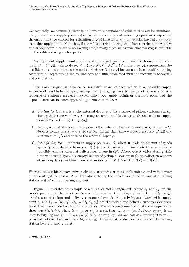
Figure 1 illustrates an example of a three-leg work assignment, where s1 and s2 are thesupply points, g is the depot, w1 is a waiting station, Ps1 = {p1, p2} and Ds1 = {d1, d2, d3}are the sets of pickup and delivery customer demands, respectively, associated with supplypoint s1 and Ps2 = {p3, p4}, Ds2 = {d4, d5, d6} are the pickup and delivery customer demands,respectively, associated with supply point s2. The work assignment consists of a sequence ofthree legs {l1, l2, l3}, where l1 = {g, p1, s1} is a starting leg, l2 = {s1, d1, d2, w1, p3, s2} is aninter-facility leg and l3 = {s2, d4, d6, g} is an ending leg. As one can see, waiting station w1

is visited between two customers (d2 and p3). However, it is also possible to visit the waitingstation before a supply point.

5


CIRRELT-2018-45

Figure 1: Example of three-leg work assignment.

The MT-PDTWCF consists of determining a set of feasible work assignments for the vehiclesto serve all customer demands. The objective is to minimize the sum of the fixed costs dueto the use of the vehicles, the routing costs for serving the customers and reaching the supplypoints, and the waiting costs at customers and supply points.

We now define the proposed mathematical formulation. Let L be the set of all feasible(starting, inter-facility and ending) legs. We denote by L+(s) the set of legs starting froms ∈ S ∪ {g}, and with L−(s) the set of legs ending at s ∈ S ∪ {g}. We define ail coefficients as

ail =

{1 if customer demand i ∈ CP ∪ CD is visited by leg l ∈ L;

0 otherwise;

and define the binary decision variables

xl =

{1 if leg l ∈ L belongs to a work assignment (i.e., is selected in the solution),

0 otherwise.

Let πl be the sum of routing and waiting costs of leg l (l ∈ L), defined as follows. LetVl = VCl ∪ VSl ∪ VWl be the set of nodes visited by l, with VCl as the set of customer demandnodes, VSl as the set of supply point nodes in l and VWl as the set of waiting stations in l. Let Albe the set of arcs belonging to l. Finally, let Tl be the set of arrival time instants θi at each nodei ∈ VCl ∪ VSl (we do not consider arrival time instants at waiting stations, as no waiting costsneed to be considered for those nodes). We define the routing cost of l as cl :=

∑(i,j)∈Al

cijand its waiting cost as wl :=

∑i∈VC

l :θi<eiσ(ei − θi) +

∑i∈VS

l :θs<t(s)−η σ(t(s) − η − θs). Then,πl := cl + wl.

6


CIRRELT-2018-45

The MT-PDTWCF can then be formulated as

Minimize∑l∈L

πlxl +∑

l∈L+(g)

Fxl (1a)

s.t.∑l∈L

ailxl = 1 ∀i ∈ CP ∪ CD (1b)∑l∈L+(g)

xl ≤ m (1c)

∑l∈L+(s)

xl =∑

l∈L−(s)

xl ∀s ∈ S (1d)

xl ∈ {0, 1} ∀l ∈ L. (1e)

The objective function (1a) minimizes the total cost of operating and using the vehicles.Constraints (1b) requires that every customer demand is performed by exactly one leg. Con-straint (1c) is the typical limit on the total number of used vehicles, indeed it bounds thenumber of work assignments to m, which is the number of available vehicles. Constraints (1d)guarantee the flow conservation at each supply point. These constraints allow combining legsinto a (multi-trip) work assignment for a vehicle. In addition, these constraints ensure that eachvehicle leaves and goes back to the depot (i.e., it is not possible to only select inter-facility legs).Note that, since we have time windows associated with the supply points and they are short(η is a small value), a work assignment cannot return to the same supply point, thus avoidingthe need for subtour elimination constraints. Finally, let us call λi, µ and γs the dual variablesassociated with constraints (1b), (1c) and (1d), respectively, with λi free (i ∈ CP ∪ CD), µ ≤ 0and γs free (s ∈ S).

4 Solution method

To solve MT-PDTWCF we propose a Branch-and-Cut-and-Price algorithm, based on ILPmodel (1). As the model contains exponentially many variables, a lower bound on the op-timal solution value is obtained by solving its Linear Programming (LP) relaxation by columngeneration. The pricing problem to derive negative reduced cost legs consists of a ResourceConstrained Elementary Shortest Path Problem (RCESPP), which is NP-hard (Dror, 1994).To solve it, we propose a bi-directional dynamic programming algorithm (see, e.g., Righiniand Salani, 2006, 2008), designed to cope with the features of MT-PDTWCF, and combinedwith effective dominance rules and label filtering to reduce the number of labels. A heuristicpricing algorithm is also developed to speed-up the column generation procedure. Two typesof inequalities, that extend powerful well-known inequalities from the literature, are appliedto significantly improve the quality of the lower bound. Finally, three branching rules aresequentially applied on fractional solutions to determine an optimal integer solution.

The proposed Branch-and-Cut-and-Price algorithm takes into account the specific featuresof MT-PDTWCF, namely multi-trip, (pickup and delivery) customer demands belonging to

7


CIRRELT-2018-45

different service zones (as defined in Section 3), and synchronization. Since a route is composedby several legs (trips), the dynamic programming algorithm computes single legs and thenthey are combined in the master problem. As we have customer demands divided into servicezones, the dynamic programming algorithm considers them separately in label propagation andthen combines labels of different zones. For the same reason, the proposed inequalities aredefined on specific service zones: this allows dealing with a smaller number of inequalities,that can be easily considered in the dynamic programming algorithm. Finally, the key issue issynchronization and how to deal with the time resource: indeed, a smaller time consumptionin a leg is not necessarily an advantage because waiting implies a cost. To tackle this issue, wedefine a particular label structure, and specific dominance rules and label filtering that allowfathoming labels to speed-up the solution process. All these features are detailed in the nextsections.

Section 4.1 describes how we initialize the solution process. Then we present the maincomponents of the algorithm: the lower bound computation with the two types of inequalitiesin Section 4.2, the pricing algorithm combined with effective dominance rules and label filteringin Section 4.3, the heuristic pricing algorithm in Section 4.4, and the branching rules in Section4.5.

4.1 Initialization

The first step of the proposed algorithm is to reduce the size of network G by removing arcsthat cannot be used in any optimal solution. In particular, for given i, j ∈ CP ∪ CD, if

ei + δ(i) + cij > lj ,

then arc (i, j) can be removed from A. Then we start with a restricted master problem, whichcontains, for each constraint (1b), a very high cost dummy variable to guarantee feasibility.

4.2 Lower bound

To compute a lower bound, we iteratively search for promising legs, i.e., variables with negativereduced cost and add them to the restricted problem. When negative reduced cost variablesno longer exist, the linear relaxation of the restricted master problem is equivalent to the LPrelaxation of model (1) and gives a valid lower bound for the MT-PDTWCF.

The pricing problem is modeled as a RCESPP, where all the feasibility constraints on theroute legs are enforced (see Section 3). We observe that each inter-facility leg is composed ofa delivery phase and a pickup phase: therefore, it is possible to compute the two partial legsindependently and then join them to find a complete leg. Each starting leg or each ending legcan be seen as a special inter-facility leg, where one of the two phases is empty. Therefore,we have a single type of pricing problem to compute all types of legs, i.e., starting, inter-facility or ending legs. Before describing, in Section 4.3, the algorithm used to find negative

8


CIRRELT-2018-45

reduced cost route legs, we explain how a stronger lower bound can be obtained by addingvalid inequalities to the linear relaxation of model (1). In particular, we consider subset-rowinequalities and rounded capacity inequalities. Both types of inequalities are adapted to dealwith MT-PDTWCF by taking into account subsets of customers (in the same or different servicezones), and are defined so as to effectively be used within the dynamic programming solutionframework. Both types of inequalities turn out to be fundamental in the solution process, as itwill be shown in Section 5.

Zone-based subset-row inequalities (ZSR3) We consider the subset-row inequalities in-troduced by Jepsen et al. (2008) for the VRP with Time Windows. In particular, we considerthe case in which subsets have cardinality three. Let C3 = {C ⊆ (CP ∪ CD) : |C| = 3} be theset of all subsets C of customer demands of cardinality 3, and, for C ∈ C3, let L(C) ⊆ L be theset of legs visiting at least 2 customer demands in C. The following inequalities are valid formodel (1): ∑

l∈L(C)

xl ≤ 1 ∀C ∈ C3. (2)

Given a subset of three customer demands, these inequalities require to select at most oneleg among all legs that visit at least two customer demands in the subset. Let us note ρCthe dual variables associated with inequalities (2), with ρC ≤ 0 (C ∈ C3). Since the numberof inequalities in (2) is polynomial in the number of customers, the separation can be easilyperformed by complete enumeration. In the Branch-and-Cut-and-Price algorithm, we performthe separation when no negative reduced cost variable can be found by the pricing algorithm.

To embed inequalities of the form (2) within the dynamic programming algorithm, insteadof considering any subset of three customer demands, we divide them into two groups:

• Intra-zone subset-row inequalities, when the three customer demands in C belong to thesame (pickup or delivery) service-zone, i.e., the three customer demands are all pickupcustomer demands or all delivery customer demands of a supply point;

• Inter-zone subset-row inequalities, when the three customer demands in C belong to dif-ferent service-zones, i.e., the three customer demands belong to service zones of differentsupply points.

Intra-zone and inter-zone inequalities will be used separately by the dynamic programmingalgorithm. In particular, intra-zone inequalities will be considered when building a partial leg ofa delivery or a pickup service zone, while inter-zone inequalities will be considered when joiningpartial legs into a complete one. We refer to Section 4.3 for further details and introduce herethe necessary notation. Given a supply point s ∈ S, we call Cintra,P3 (s) = {C ⊆ CPs : |C| = 3}the set of subsets of pickup customer demands of cardinality 3 that induce intra-zone subset-row inequalities, and Cintra,D3 (s) = {C ⊆ CDs : |C| = 3} the set of subsets of delivery customerdemands of cardinality 3 that induce intra-zone subset-row inequalities. Given a pair of supplypoints s, s′ ∈ S, we call Cinter3 (s, s′) = {C ⊆ (CDs ∪CPs′ ) : |C| = 3, |C ∩CDs | ≥ 1, |C ∩CPs′ | ≥ 1} the

9


CIRRELT-2018-45

set of subsets of customer demands of cardinality 3, with at least one customer in the deliveryzone of s and another customer in the pickup zone of s′, that induce inter-zone subset-rowinequalities.

Zone-based rounded-capacity inequalities (ZCAP) Rounded capacity inequalities arewell known valid inequalities for routing problems (see Naddef and Rinaldi, 2002), which requireall subsets of customers to be served by enough vehicles. Instead of considering any subset ofcustomers, we consider a special case of such inequalities in which the set of customers containseither all the pickup customer demands or all the delivery customer demands of a supply point.When we consider all the pickup customer demands associated with a supply point s ∈ S, theinequalities take the form:

∑l∈L−(s)

xl ≥

⌈∑i∈CPs qi

Q

⌉∀s ∈ S. (3)

They require that the number of legs visiting pickup customer demands to be served by supplypoint s is at least the rounded ratio of the sum of the pickup customer demands over the capacityof the vehicle. Similar inequalities can be written for the delivery customer demands. Note thatwe define the rounded capacity inequalities on a delivery service zone or on a pickup service zone:this allows to easily deal with these inequalities within the dynamic programming algorithm(see Section 4.3). In addition, having defined these inequalities on the service zones allows tohave a small number of inequalities: thus, they are directly added to the master problem beforestarting the column generation procedure. We denote ξPs the dual variables associated withinequalities (3), referred to pickup customers, and ξDs the dual variables associated with thesame inequalities but referred to delivery customers, with ξPs ≥ 0 and ξDs ≥ 0 (s ∈ S).

4.3 Pricing algorithm

Dynamic programming techniques are very effective in solving RCESPPs, and, in particular,we focus on bi-directional extension of node labels (Righini and Salani, 2006, 2008), which isbased on forward and backward label propagation. Labels are associated with nodes of G. Theproposed dynamic programming algorithm applies bi-directional extension of node labels, whichwe designed to effectively cope with multi-trip, service zones and synchronization features thatrequired ad hoc adaptations of the standard framework. In the following we report the pricingproblem, and describe label structure, propagation, join of labels, dominance rules, and labelfiltering.

Pricing problem. The pricing problem calls for finding a negative reduced cost feasible legl ∈ L. We first describe the pricing problem for an inter-facility leg l ∈ L with supply pointss, s′ ∈ S, and then explain the changes to deal with starting or ending legs. As before, we letVl = VCl ∪ VSl ∪ VWl be the set of nodes visited by l, with VCl as the set of customer demandnodes, VSl as the set of supply point nodes in l and VWl as the set of waiting stations in l, and Al

10


CIRRELT-2018-45

be the set of arcs belonging to l. Finally, Tl indicates the set of arrival time instants θi at eachnode i ∈ VCl ∪VSl (also here, we do not consider arrival time instants at waiting stations, since no

waiting costs need to be considered at these nodes). In addition, we define C∗,lintra,D(s), C∗,lintra,P(s)

and C∗,linter(s, s′) as the sets of all subsets of customer demands of cardinality 3 that induce,respectively, delivery intra-zone, pickup intra-zone and inter-zone subset-row inequalities, suchthat at least two customer demands are visited by leg l: C∗,lintra,D(s) = {C ∈ Cintra,D3 (s) :

|Vl∩C| ≥ 2}, C∗,lintra,P(s) = {C ∈ Cintra,P3 (s) : |Vl∩C| ≥ 2} and C∗,linter(s, s′) = {C ∈ Cinter3 (s, s′) :|Vl ∩ C| ≥ 2}. The pricing problem is to find a leg l ∈ L, satisfying feasibility conditionsdescribed in Section 3, such that it has negative reduced cost:

∑(i,j)∈Al

cij +∑

i∈VCl :θi<ei

σ(ei − θi) +∑

i∈VSl :θs<t(s)−η

σ(t(s)− η − θs)

−∑i∈VC

l

λi − γs + γs′

−∑

C∈C∗,lintra,D(s)

ρC −∑

C∈C∗,lintra,P (s′)

ρC −∑

C∈C∗,linter(s,s′)

ρC − ξDs − ξPs′ < 0.

(4)

In the first line we can see the routing and waiting cost of the leg, the second line takes intoaccount the dual variables of constraints (1b) and (1d), while the last line considers the dualvariables of the intra-zone and inter-zone subset-row inequalities and of the rounded capacityinequalities. Recall that the latter ones are inserted in the master before starting the columngeneration procedure, while subset-row inequalities are separated by enumeration.

If we consider a starting leg, we need to add F − µ to the reduced cost, as the fixed cost ofthe vehicle and the dual variable of constraint (1c) need to be taken into account. In addition,for a starting leg from g to s′, we do not have the terms including dual variables referred to s,while, for an ending leg from s to g, we do not have the terms including dual variables referredto s′.

To solve this problem, we developed a dynamic programming algorithm. We consider eachdelivery and pickup service zone of a supply point s ∈ S. Labels are propagated forward fromeach supply point s to its delivery customers i ∈ CDs (delivery service zone) and backward to itspickup customers j ∈ CPs (pickup service zone). In particular, forward labels represent pathsfrom s to i and backward labels represent paths from j to s. Each label includes informationon its resource consumption (e.g., time, vehicle capacity), visited customers and reduced cost.Each label is iteratively considered and the corresponding path is extended to adjacent nodes.Note that, in the extension, we need to consider both the direct arc between two nodes and thepossibility to stop at a waiting station in between.

Forward and backward labels belonging to zones of different supply points are joined inpairs to form complete legs. Before giving details on the label structure, we explain the mainnovelties of the dynamic programming algorithm.

11


CIRRELT-2018-45

As mentioned above, multi-trip, service zones and synchronization features need to be care-fully handled in the bi-directional extension of node labels. Since we have multi-trips and(delivery and pickup) customer demands associated with specific supply points, it is importantto consider delivery and pickup service zone separately in the label extension and combine themthrough the joining of labels. This also allows to effectively deal with subset-row and rounded-capacity inequalities. Moreover, we need to consider the opportunity of visiting waiting stationswhen extending labels of a delivery or a pickup service zone, and when joining labels of differentsupply points. Another issue consists of the way to cope with synchronization and time con-sumption. Due to the synchronization constraints and to the additional flexibility of waitingat supply points or customers that we allow, a smaller time consumption is not necessarily anadvantage when evaluating states of the dynamic programming: indeed, it might imply largerwaiting costs when propagating to other nodes. On the other hand, a larger time consumptionis clearly a limitation, as in classical routing problems with time windows, since it might inhibitto visit some nodes. Thus, there might be an infinite number of non-dominated states asso-ciated with the same path, having the same cost, but different time consumptions, obtainedby delaying the departure time from a waiting station (or from the depot). To cope with thisissue, we group them into a single label by introducing an additional resource φ representingthe forward shift of the label, i.e., the amount of delay that can be introduced without violatingthe time window constraints of the visited customers.

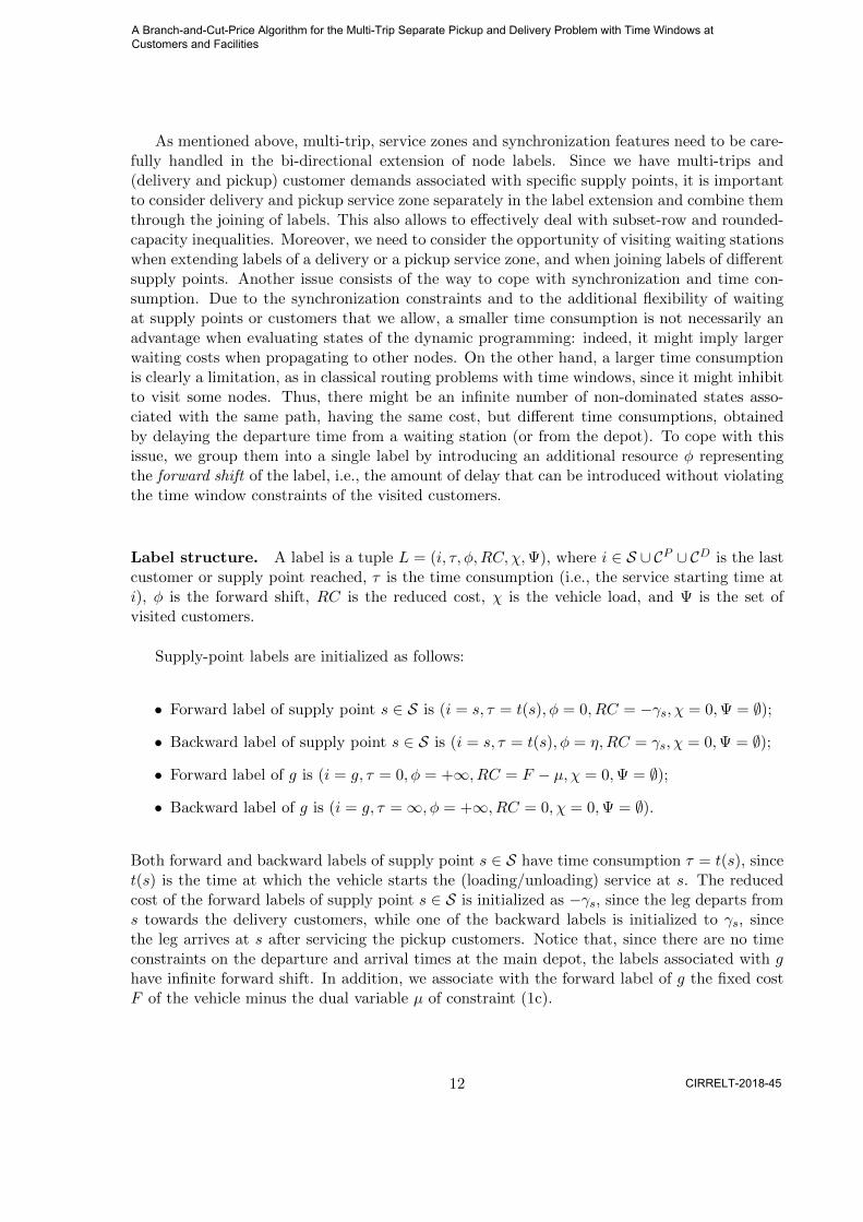
Label structure. A label is a tuple L = (i, τ, φ,RC, χ,Ψ), where i ∈ S ∪ CP ∪ CD is the lastcustomer or supply point reached, τ is the time consumption (i.e., the service starting time ati), φ is the forward shift, RC is the reduced cost, χ is the vehicle load, and Ψ is the set ofvisited customers.

Supply-point labels are initialized as follows:

• Forward label of supply point s ∈ S is (i = s, τ = t(s), φ = 0, RC = −γs, χ = 0,Ψ = ∅);

• Backward label of supply point s ∈ S is (i = s, τ = t(s), φ = η,RC = γs, χ = 0,Ψ = ∅);

• Forward label of g is (i = g, τ = 0, φ = +∞, RC = F − µ, χ = 0,Ψ = ∅);

• Backward label of g is (i = g, τ =∞, φ = +∞, RC = 0, χ = 0,Ψ = ∅).

Both forward and backward labels of supply point s ∈ S have time consumption τ = t(s), sincet(s) is the time at which the vehicle starts the (loading/unloading) service at s. The reducedcost of the forward labels of supply point s ∈ S is initialized as −γs, since the leg departs froms towards the delivery customers, while one of the backward labels is initialized to γs, sincethe leg arrives at s after servicing the pickup customers. Notice that, since there are no timeconstraints on the departure and arrival times at the main depot, the labels associated with ghave infinite forward shift. In addition, we associate with the forward label of g the fixed costF of the vehicle minus the dual variable µ of constraint (1c).

12


CIRRELT-2018-45

Figure 2: Example of forward label propagation.

Label propagation. We describe in detail the extension rules for forward labels, i.e., froma delivery customer label to another delivery customer label or from a supply point label to adelivery customer label. Similar rules are applied in the backward search.

When a label L = (i, τ, φ,RC, χ,Ψ), associated with node i ∈ CDs , is extended to nodej ∈ CDs , the new label L′ = (j, τ ′, φ′, RC ′, χ′,Ψ′) is computed according to the following rules:

τ ′ = max{τ + δ(i) + cij , ej} (5a)

φ′ = max{0,min{φ− ν, lj − τ ′}} (5b)

RC ′ = RC + cij − λj + σω (5c)

χ′ = χ+ qj (5d)

Ψ′ = Ψ ∪ {j}, (5e)

where ν = max{ej− (τ + δ(i)+ cij), 0} is the waiting time and ω = max{ν−φ, 0} is the waitingtime reduced by φ, since φ can (partially or fully) absorb it. In label L′, the time consumptionτ is increased by the service time duration δ(i) at node i plus the routing time cij from i to j.If this value is smaller than ej , then the vehicle will wait at node j, and the time consumptionis set equal to ej . The forward shift φ′ (that must be greater or equal to zero) is set as theminimum between the previous forward shift φ decreased by waiting time ν and lj−τ ′. Indeed,φ′ is the remaining amount of delay, after visiting customer j, that can be introduced withoutviolation of the time window constraints of the customers in Ψ′. The reduced cost is updatedby adding the routing and waiting costs, and subtracting the dual variable λj of the visitedcustomer j. Finally, the vehicle load is increased by the customer demand qj , and j is addedto the visited customers.

We show in Figure 2 an example of forward label propagation: top, we can see the timewindow [ei, li] of label L and, bottom, the time window [ej , lj ] of label L′. In L, we have a timeconsumption τ and a forward shift φ. The arrow from τ indicates the arrival time at node j,i.e., τ + δ(i) + cij . As we can see, the vehicle arrives earlier than ej and therefore must waitfor time ν. However, the forward shift φ can be used to reduce the waiting time at j. Thus,the reduced cost RC ′ takes into account the waiting cost σω. In this example, the new timeconsumption τ ′ is set to ej , and the new forward shift φ′ becomes zero.

13


CIRRELT-2018-45

When a label L = (i, τ, φ,RC, χ,Ψ), associated with node i ∈ S is extended to nodej ∈ CDs , the same computation is performed except for the time consumption that is set toτ ′ = max{τ + ϕ(i) + cij , ej}.

As described earlier, vehicles can stop at waiting stations instead of going directly from onecustomer to another. If a label of customer i is extended to customer j through the waitingstation w, the new label is computed as:

τ ′ = max{τ + δ(i) + ciw + cwj , ej} (6a)

φ′ = lj − τ ′ (6b)

RC ′ = RC + ciw + cwj − λj (6c)

χ′ = χ+ qj (6d)

Ψ′ = Ψ ∪ {j}. (6e)

Note that, we need the routing cost ciw + cwj for going from node i to the waiting station wand then to node j. In this case, the vehicle never waits at customer j (since it can wait atthe waiting station at no cost), thus φ′ = lj − τ ′. Given a pair of customers i and j, the mostconvenient waiting station where to stop is w ∈ argminw∈W{ciw + cwj}. This value ciw + cwjdoes not depend on the dual variables. Hence, we precompute w for each pair of customers.

The label L′ is feasible if

j /∈ Ψ

τ ′ ≤ ljχ′ ≤ Q.

At the end of the search phase, intra-zone subset-row inequalities are evaluated and thereduced cost of the labels are updated accordingly. In particular, let

C∗intra,D(s) ={C ∈ Cintra,D3 (s) : |Ψ′ ∩ C| ≥ 2

}, i.e., C∗intra,D(s) is the set of all subsets of delivery

customer demands of cardinality 3 that induce intra-zone subset-row inequalities, such that atleast two delivery customer demands are visited by the partial leg corresponding to label L′.The reduced cost RC ′ is updated as RC ′ −

∑C∈C∗intra,D(s) ρC .

Join. In order to obtain complete (starting, ending or inter-facility) route legs, forward andbackward labels of delivery and pickup service zones of different supply points are joined inpairs. In other words, the join operation is used to join a label of a delivery service zone of asupply point s with a label of a pickup service zone of a supply point s′. Let us consider thejoin between a label Lfw = (i, τfw, φfw, RCfw, χfw,Ψfw) of delivery customer i ∈ CDs and labelLbw = (j, τbw, φbw, RCbw, χbw,Ψbw) of pickup customer j ∈ CPs′ . The two labels Lfw and Lbware compatible if

τfw + δ(i) + cij ≤ τbw.

Indeed, it is necessary that the service starting time τfw at i, plus the service time δ(i) andthe routing cost cij from i to j, be smaller or equal to the service starting time τbw at j. Since

14


CIRRELT-2018-45

the two labels are linked to different service zones, the two labels have visited disjoint sets ofcustomers. Also, the vehicle load resources are always compatible: the forward label performsdelivery operations, while the backward label performs pickup operations. Thus at the joinpoint the vehicle is empty.

Let s and s′ be the starting supply points of Lfw and Lbw, respectively, and let ξDs andξPs′ be the dual variables of the rounded capacity inequalities associated with the deliveryservice zone of s and with the pickup service zone of s′, respectively. Also, let C∗inter(s, s′) ={C ∈ Cinter3 (s, s′) : |(Ψfw ∪Ψbw) ∩ C| ≥ 2

}, i.e., C∗inter(s, s′) is the set of all subsets of customer

demands of cardinality 3 that induce inter-zone subset-row inequalities, such that at least twocustomer demands are visited by the leg, between s and s′, that will result from the join oflabels Lfw and Lbw.

The reduced cost of the route leg resulting from the join of Lfw and Lbw is

RCfw − ξDs + cij + σω − ξPs′ +RCbw −∑

C∈C∗inter(s,s′)

ρC ,

where ω denotes the necessary waiting time between i and j that cannot be absorbed by theforward shift of both labels. It is defined as

ω = max{0, τbw − (τfw + cij + δ(i))− (φbw + φfw)}.

Indeed, the waiting time at node j is given by the difference between the service starting timeτbw at j, minus the sum of the ending time of service τfw + δ(i) at i, plus the routing time cijbetween the two nodes, reduced by the sum of the forward shifts φfw + φbw.

As previously, it is necessary also for the join to consider the possibility to stop at a waitingstation w ∈ W. In this case, the feasibility condition for the join is

τfw + δ(i) + ciw + cwj ≤ τbw

and the resulting reduced cost is

RCfw − ξDs + ciw + cwj − ξPs′ +RCbw −∑

C∈C∗inter(s,s′)

ρC .

Notice that, to obtain a complete starting leg, the join operation is applied between abackward label of a supply point s ∈ S and the label of g, while to obtain a complete endingleg the join operation is applied between the label of g and a forward label of a supply points ∈ S. After joining, we discard all the labels with RC ≥ 0.

Dominance rules. Effective dominance rules, capable of fathoming a large number of labels,are a fundamental ingredient in a labeling algorithm for the RCESPP. As mentioned above,it is not easy to detect whether a larger time consumption is an advantage or a disadvantagewhen comparing labels. Hence, in principle, only labels with the same time consumption can

15


CIRRELT-2018-45

be directly compared. This limitation significantly reduces the number of labels that can befathomed. We use the two following dominance rules that combine the information on timeconsumption, cost and forward shift to compare labels with different time consumption. WithDominance Rule 1, we try to dominate a label L′′ with a label L′ by allowing to wait at thecustomer (if necessary), and thus paying the corresponding waiting cost. With Dominance Rule2, we try to dominate a label L′′ with a label L′ by allowing to wait at a waiting station w.Recall that waiting at a waiting station is possible at any time and there is no restriction onthe number of waiting stations visited. These two dominance rules are applied in sequence (oneafter the other) and guarantee that only dominated labels are removed. Note that the twodominance rules are independent of each other. More precisely, if at least one of the two rulescan be applied, label L′′ is dominated by label L′ and can be removed.

Proposition 1 (Dominance Rule 1). A forward label L′ = (i, τ ′, φ′, RC ′, χ′,Ψ′), with i ∈ CDs ,dominates a forward label L′′ = (j, τ ′′, φ′′, RC ′′, χ′′,Ψ′′) if

i = j

τ ′ ≤ τ ′′

RC ′ + σmax{0, τ ′′ + φ′′ − (τ ′ + φ′)} ≤ RC ′′

χ′ ≤ χ′′

Ψ′ ⊆ Ψ′′.

(7)

The term σmax{0, τ ′′ + φ′′ − (τ ′ + φ′)} is the cost incurred by label L′ to wait until timeτ ′′ + φ′′, the latest feasible service starting time for label L′′. In other words, it is not enoughto have RC ′ ≤ RC ′′, since L′′ might have more possibilities to delay without violating the timewindow constraints of the visited customers. Therefore, we consider the time needed in L′ toreach the latest feasible service starting time of L′′, and evaluate the corresponding waitingcost. If RC ′ increased by this cost is still smaller or equal to RC ′′, then L′′ is dominated.

Proposition 2 (Dominance Rule 2). A forward label L′ = (i, τ ′, φ′, RC ′, χ′,Ψ′), with i ∈ CDs ,dominates a forward label L′′ = (j, τ ′′, φ′′, RC ′′, χ′′,Ψ′′) if

i = j

τ ′ + maxh∈CDs {minw∈W{ciw + cwh − cih}} ≤ τ ′′

RC ′ + maxh∈CDs {minw∈W{ciw + cwh − cih}} ≤ RC ′′

χ′ ≤ χ′′

Ψ′ ⊆ Ψ′′.

(8)

Here, maxh∈CDs {minw∈W{ciw + cwh − cih}} is the maximum routing time (and cost) over

all possible next customers h ∈ CDs , which can be reached by visiting a waiting station beforeh. Dominance Rule 2 is used to dominate labels by considering the possibility of visiting awaiting station from the current node i before visiting the next node h. Instead of directlygoing from node i to node h (at cost cih), we consider the possibility of going from node i tothe best waiting station for pair i, h (at cost ciw + cwh). If the time consumption τ ′ increasedby the maximum additional routing time towards/from the waiting station is still smaller or

16


CIRRELT-2018-45

equal to τ ′′ and the reduced cost RC ′ increased by the maximum additional routing cost isstill smaller or equal to RC ′′, then L′′ is dominated. The waiting station is chosen such thatit is the most convenient for customers i and h, and the additional routing time (and cost) toreach customer h through the waiting station is chosen as the maximum one among all possiblecustomers (since L′ dominates L′′ only if the worst situation is considered). Note that it isalways possible to go to a waiting station later than immediately after customer i, but, sincewaiting stations have no limit on the number of visits, we can dominate label L′′ as describedabove without checking what happens afterwards.

Similar dominance rules can be defined for backward labels. Dominance rules are appliedduring the label propagation, i.e., we check if a label is dominated by other labels beforeextending it.

Filtering final labels. Once the label propagation phase is terminated, and before applyingthe join operation, it is possible to filter the final labels using more effective dominance rules,which require weaker conditions to be satisfied. In particular, it is possible to drop conditionson the load of the vehicle and on the set of visited customer demands. By removing theseconditions, we are able to dominate additional labels. Recall that join is applied to combinea label of a delivery service zone and a label of a pickup service zone. Therefore, joiningoccurs with an empty vehicle and it is not necessary to check the vehicle load for final labels. Inaddition, forward and backward propagations operate on disjoint sets of customer demands and,thus, joining a forward label and a backward label never causes visiting a customer demandmore than once. This allows removing the condition on the visited customer set. However,since inter-zone inequalities are used, they must be taken into account in this phase. Indeed,these inequalities contribute to increase the reduced cost. In particular, we add to the labels anadditional resource αC for each inequality C ∈ ∪s′∈S,s′ 6=sCinter3 (s, s′), where s ∈ S is the supplypoint of the considered label. The value of αC represents the number of customer demandsof the considered label that are involved in inequality C. We apply the following rule for thefiltering of final labels: A forward final label L′ = (i, τ ′, φ′, RC ′, χ′,Ψ′), with i ∈ CDs , dominatesa forward final label L′′ = (j, τ ′′, φ′′, RC ′′, χ′′,Ψ′′) if

i = j

τ ′ ≤ τ ′′

RC ′ + σmax{0, τ ′′ + φ′′ − (τ ′ + φ′)} ≤ RC ′′

α′C ≤ α′′C ∀C ∈ ∪s′∈S,s′ 6=sCinter3 (s, s′).

(9)

In other words, it is not necessary to check that Ψ′ ⊆ Ψ′′, but only that α′C ≤ α′′C , ∀C ∈∪s′∈S,s′ 6=sCinter3 (s, s′). Indeed, if the number α′C of customer demands involved in an inter-zoneinequality C for label L′ is smaller or equal to the number α′′C of customer demands involvedin the same inequality for label L′′, the contribution of the dual variable ρC is either the samein both labels or it is larger for L′′. Thus, since ρC ≤ 0, this ensures dominance of L′ over L′′,provided that the other conditions above are satisfied.

17


CIRRELT-2018-45

4.4 Heuristic pricing algorithm

In order to speed-up the column generation procedure, we developed a heuristic pricing al-gorithm (HP). It is similar to the exact pricing algorithm described in Section 4.3, but usesrelaxed dominance rules to fathom a larger number of non-promising labels. More precisely,the check on the set of visited customers Ψ′ ⊆ Ψ′′ is removed from both rules (7) and (8). HPis used to quickly find negative reduced cost legs. We noticed, during preliminary experiments,that the failure rate of HP in finding negative reduced cost columns increases when subset-rowinequalities are added to the master problem. Hence, we use HP in the initial iterations ofcolumn generation and stop calling it as subset-row inequalities are generated. Clearly, theexact pricing algorithm is applied to derive a valid lower bound, when HP is not able to find anegative reduced cost column.

4.5 Branching rules

We consider three branching rules to be applied alternatively when a fractional solution isfound. The first one limits the total number of vehicles, the second one imposes bounds on thenumber of vehicles visiting a supply point, and the third branching rule fixes or forbids an arc.

Let v =∑

l∈L+(g) xl be the number of vehicles used in the optimal solution of the linearrelaxation master problem. When v is fractional, we impose in one branch to use at most bvcand at least dve vehicles in the other. This branching decision can be enforced by introducinga constraint of the form ∑

l∈L+(g)

xl ≤ bvc

or ∑l∈L+(g)

xl ≥ dve

in the master problem and it does not affect the structure of the pricing problem. Indeed, wehave an additional constraint whose dual variable can be taken into account, in a similar wayas variable µ, in the initialization of the forward and backward labels of the depot g.

When an integer number of vehicles is used, we search for a supply point s ∈ S visited bya fractional number of vehicles. Let vs =

∑l∈L+(s) xl be the number of vehicles visiting supply

point s ∈ S in the optimal solution of the linear master problem; we perform a binary branchingsimilar to the previous case, by adding to the master problem one of the following constraintsin each child subproblem: ∑

l∈L+(s)

xl ≤ bvsc

or ∑l∈L+(s)

xl ≤ dvse.

18


CIRRELT-2018-45

When there are multiple supply points with fractional vehicle flow, the one with the fractionalpart closest to 0.5 is selected, as it often yields a stronger effect on the fractional solution whenbranching. The structure of the pricing problem is not destroyed in this case as well.

When no supply point has fractional vehicle flow, we branch on the arc selection. Wecompute the flow on the arcs corresponding to the optimal fractional solution of the masterproblem, and select the arc (i, j) whose flow is the closest to 0.75. Arcs with integer flow arenot considered. Arc (i, j) is forbidden in one branch. The arc is then removed from G and, inthe dynamic programming procedure, labels of node i will not be extended to node j. In thisway, the pricing algorithm will not produce any route leg containing (i, j). All the variablesalready present in the master problem associated with route legs visiting i and j in sequence(even if stopping at a waiting station in between) are discarded as well. We impose to use arc(i, j) in the second branch. This is enforced by removing from G the arcs (i, j′) for j 6= j′ andby removing from the master problem all the variables associated with route legs vising vertexi followed by a vertex different from j. Since this branching rule has generally a weaker impacton fractional solutions, it is only used when the two previous rules cannot be applied.

5 Experimental analysis

The aim of our experiments is to analyze the performance of the proposed Branch-and-Cut-and-Price algorithm. In particular, we first evaluate the impact of the proposed zone-basedsubset-row and zone-based rounded capacity inequalities on the computation of the lower boundat the root node (Section 5.2). Then, we report the results obtained by the Branch-and-Cut-and-Price algorithm (Section 5.3). Finally, in Section 5.4, we consider other problem settingsof MT-PDTWCF.

The algorithm described in Section 4 has been implemented in C++ using SCIP 4.0.1, linkedto CPLEX 12.6.1, as a Branch-and-Cut-and-Price framework. All parameters are set at theirdefault values, except from preprocessing and automatic cut generation that are not used. Allexperiments are executed on an Intel i7-3820, 3.6GHz workstation by using a single core.

5.1 Test instances

We generated seven sets of 10 problem instances, using the same parameters proposed in Crainicet al. (2015b) and Nguyen et al. (2017). The first three sets, called D1-D3, have the same numberof supply points and different number of customers per service zone. The following three sets,called D4-D6, instead, have the same number of customers per service zone, but a differentnumber of supply points. Finally, the last set, called E1, has 10 supply points and an averageof 10 pickup and 10 delivery demands for each service zone. We decided to identify the last setwith a different letter, because the larger number of customers per service zone makes themconsiderably more difficult than the previous six sets.

19


CIRRELT-2018-45

We consider a square of size 200 where customers, supply points, and waiting stations areuniformly distributed. The opening time of the supply points is randomly generated in theinterval [0, 14400]. The parameters η and ϕ are set to 100 and 30 respectively. The number ofvehicles m is set to 50.

Customers are assigned to supply points based on their proximity. More precisely a customeris assigned to its first, second, third and fourth nearest supply point with probability 0.5, 0.25,0.15, and 0.1, respectively. The ready time of a delivery customer is computed as the sum ofthe opening time of the corresponding supply point, the loading time at the supply point, therouting time between the supply point and the customer, and a random value in the interval[0, 300]. The time window duration is uniformly selected in the [150, 450] range. Similarly, thedue date of a pickup customer is generated by subtracting the service time at the customer,the routing time from the customer to the supply point, and a random value in the interval[0, 300] from the opening time of the supply point. The service time of all customers is set to20. The demand of each customer is randomly generated in the interval [5, 25] and the vehiclecapacity is set to 100. The main depot is set at the middle point of the square. A fixed costF = 500 is accounted for each vehicle used. Waiting at customer and supply points is allowedwith a penalty σ = 0.5. All parameters used for generating these instances are the same as inCrainic et al. (2015b) and Nguyen et al. (2017), except from the waiting cost σ that has beenintroduced to adapt the instances to MT-PDTWCF.

The description of the datasets is summarized in Table 1.

dataset |S| cust/zone cust demands

D1 5 5 50D2 5 7 70D3 5 9 90D4 5 6 60D5 10 6 120D6 15 6 180E1 10 10 200

Table 1: Datasets description

The time limit was set to one hour in all tests with D1-D6 and to two hours in all tests withE1.

5.2 Lower bound

We have considered four configurations: the linear relaxation of model (1) without any addi-tional cut (no cuts in Table 2), with zone-based subset-row inequalities (ZSR3), with zone-basedrounded-capacity inequalities (ZCAP), and with both. The results are summarized in Table2. The average percentage gap with respect to the optimal solution values and the averagecomputing time, expressed in seconds, are reported for each configuration and each class of

20


CIRRELT-2018-45

no cuts ZSR3 ZCAP ZSR3+ZCAP

class gap time gap time gap time gap time

D1 6.83% 0.17 1.40% 0.89 1.99% 0.16 0.00% 0.60D2 11.62% 0.91 0.68% 16.91 2.59% 0.58 0.39% 2.98D3 8.65% 7.37 1.04% 238.82 5.24% 5.03 1.03% 150.47D4 10.59% 0.39 1.44% 5.06 1.30% 0.32 0.52% 0.55D5 8.28% 2.42 1.24% 12.44 2.23% 1.57 0.84% 2.70D6 7.87% 7.96 0.86% 28.87 2.20% 5.57 0.63% 9.76E1 6.83% 158.61 1.51% 3042.55 4.15% 122.14 0.26% 1878.38

avg. all 8.67% 25.40 1.17% 477.93 2.81% 19.34 0.52% 292.21

Table 2: Lower bound evaluation.

instances. We report in the last row the average values of gaps and computing times over allclasses of instances.

Without valid inequalities, the linear relaxation of model (1) gives a rather weak bound(the average gap is 8.67% on all instances). Zone-based subset-row inequalities are able toconsiderably improve the lower bound, reducing the average gap to 1.17%, but the computingtimes increase, especially on class D3 and E1 (recall that we allow two hours of time limit forE1 instances, and one hour for D instances). The zone-based rounded-capacity inequalities arealso effective in reducing the duality gap, even if not as much as ZSR3, and the computingtime often decreases. We recall that such inequalities are added to the master problem sincethe beginning and they seem to significantly help a fast convergence of the column generationprocedure. We achieve the strongest bound (the average gap is about 0.5%) within reasonablecomputing times (292 seconds on average) using both types of inequalities (2) and (3). As it canbe seen from Table 2, the proposed valid inequalities are crucial to allow solving the problemto optimality. Indeed, the average gap reduces from 8.67% to 0.52%, thus significantly limitingthe number of branch-and-bound nodes that need to be explored, as it will be shown in Section5.3.

As frequently happens with exact algorithms, the variance of the gap values reported inTable 2 can be large. However, we observed a drastic reduction of the variance when the validinequalities are present. Hence, the configuration with both ZSR3 and ZCAP is the one weused in the Branch-and-Cut-and-Price algorithm.

5.3 Branch-and-Cut-and-Price

Table 3 reports the results obtained on the seven classes of instances by the Branch-and-Cut-and-Price algorithm described in Section 4. We report for each class of instances, the averagegap and computing time at the root node, the average gap when the time limit is reached,the average number of explored nodes for the solved instances, the average computing time

21


CIRRELT-2018-45

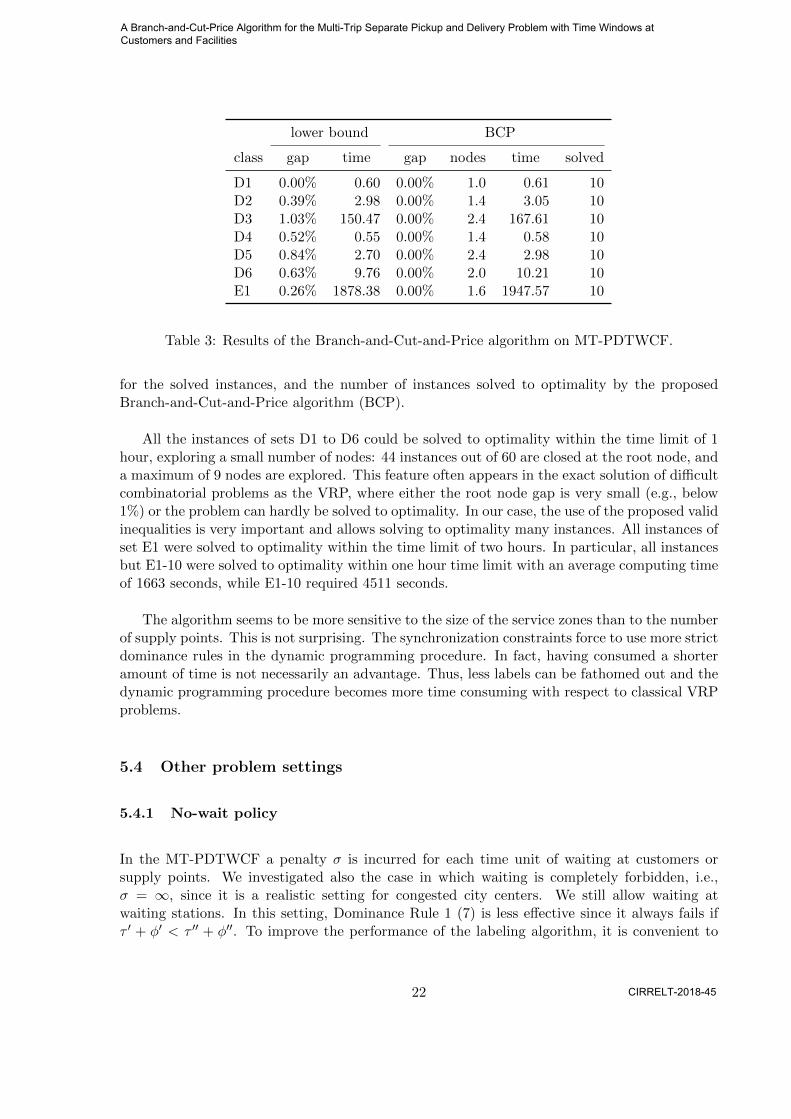
lower bound BCP

class gap time gap nodes time solved

D1 0.00% 0.60 0.00% 1.0 0.61 10D2 0.39% 2.98 0.00% 1.4 3.05 10D3 1.03% 150.47 0.00% 2.4 167.61 10D4 0.52% 0.55 0.00% 1.4 0.58 10D5 0.84% 2.70 0.00% 2.4 2.98 10D6 0.63% 9.76 0.00% 2.0 10.21 10E1 0.26% 1878.38 0.00% 1.6 1947.57 10

Table 3: Results of the Branch-and-Cut-and-Price algorithm on MT-PDTWCF.

for the solved instances, and the number of instances solved to optimality by the proposedBranch-and-Cut-and-Price algorithm (BCP).

All the instances of sets D1 to D6 could be solved to optimality within the time limit of 1hour, exploring a small number of nodes: 44 instances out of 60 are closed at the root node, anda maximum of 9 nodes are explored. This feature often appears in the exact solution of difficultcombinatorial problems as the VRP, where either the root node gap is very small (e.g., below1%) or the problem can hardly be solved to optimality. In our case, the use of the proposed validinequalities is very important and allows solving to optimality many instances. All instances ofset E1 were solved to optimality within the time limit of two hours. In particular, all instancesbut E1-10 were solved to optimality within one hour time limit with an average computing timeof 1663 seconds, while E1-10 required 4511 seconds.

The algorithm seems to be more sensitive to the size of the service zones than to the numberof supply points. This is not surprising. The synchronization constraints force to use more strictdominance rules in the dynamic programming procedure. In fact, having consumed a shorteramount of time is not necessarily an advantage. Thus, less labels can be fathomed out and thedynamic programming procedure becomes more time consuming with respect to classical VRPproblems.

5.4 Other problem settings

5.4.1 No-wait policy

In the MT-PDTWCF a penalty σ is incurred for each time unit of waiting at customers orsupply points. We investigated also the case in which waiting is completely forbidden, i.e.,σ = ∞, since it is a realistic setting for congested city centers. We still allow waiting atwaiting stations. In this setting, Dominance Rule 1 (7) is less effective since it always fails ifτ ′ + φ′ < τ ′′ + φ′′. To improve the performance of the labeling algorithm, it is convenient to

22


CIRRELT-2018-45

lower bound BCP


D1 0.00% 0.61 0.00% 1.0 0.62 10D2 0.36% 2.67 0.00% 1.4 2.75 10D3 0.83% 207.40 0.00% 2.2 233.88 10D4 0.55% 0.48 0.00% 1.6 0.51 10D5 0.92% 2.21 0.00% 3.4 2.95 10D6 0.58% 8.90 0.00% 114.9 33.69 10E1 19.35% 4683.41 19.08% 2.7 3865.63 7

Table 4: Results of the Branch-and-Cut-and-Price algorithm with no-wait policy.

block a label extension ifτ ′ + φ′ + δ(i) + cij < ej .

This means that we avoid propagating a label from node i to node j if it implies waiting atthe customer j. Of course it is still possible to extend the label from i to j through a waitingstation.

The results obtained on the seven classes of instances are summarized in Table 4. The tablehas the same structure of the previous one. The Branch-and-Cut-and-Price algorithm is againable to solve all the 60 instances in classes D1 to D6. Seven instances in class E1 could besolved within the time limit of two hours. However, for three E1 instances the algorithm wasstill processing the root node after two hours of computing time: in this case, the quality of theheuristic solution obtained by SCIP was very poor. Indeed, we can observe that the number ofnodes to determine the optimal solution is usually rather small, and many instances can directlybe solved to optimality at the root node. When the root node computation is completed,finding a good quality heuristic solution turns out to be easier for the SCIP solver. However,the solution process of the root node requires long computing times for the E1 instances andthis leads to larger gaps. E1 instances are more difficult mainly due to the larger number ofcustomers in each service zone: this difficulty is more evident in this setting due to the weaknessof dominance rule (7), as explained above.

5.4.2 Configuration of Nguyen et al. (2017)

We have experimented the behavior of the Branch-and-Cut-and-Price algorithm with a thirdproblem setting, where the stop at waiting stations is possible only immediately before goingto a supply point. Waiting at customer and supply points is allowed with a penalty (σ = 0.5).This setting corresponds to the one used in Nguyen et al. (2017). In this setting, we inserta cutoff given by the upper bound computed by the tabu search proposed in Nguyen et al.(2017). The obtained results are reported in Table 5. We can see that all but three instancesin class D3 are solved to optimality. This class is the most difficult for BCP in this setting,since it has the largest number of customers in each service zone. Restricting the possibility of

23


CIRRELT-2018-45

lower bound BCP


D1 0.38% 0.12 0.00% 3.80 0.14 10D2 0.86% 11.56 0.00% 393.30 76.31 10D3 1.12% 2046.65 0.9% 2.71 1622.75 7D4 0.38% 0.37 0.00% 2.0 0.42 10D5 0.51% 3.43 0.00% 413.70 26.80 10D6 0.72% 6.53 0.00% 534.30 42.46 10

Table 5: Results of the Branch-and-Cut-and-Price algorithm on the configuration in Nguyenet al. (2017).

going to a waiting station only right before a supply point creates more opportunities to tradewaiting costs with routing costs in the dynamic programming, thus making the dominance ruleless effective.

5.5 Solution analysis

We analyze the characteristics of the optimal solutions obtained for the three problem settings.In particular, we report in Table 6, for each of the three problem settings considering onlythe instances solved to optimality, the average number of used vehicles, the average number ofperformed legs, the average number of legs per vehicle, the average fixed cost, routing cost andwaiting cost.

We can see that the average numbers of used vehicles and legs are similar in the standardand in the no wait settings. However, larger routing costs clearly arise in the latter setting,since waiting at customers and supply point is forbidden, and the vehicle needs to travel to awaiting station. We also observe that, for all classes, the total routing and waiting cost in thestandard setting is smaller (about 3% on average) than the routing cost in the no wait setting.Therefore, the flexibility of waiting at customers and supply points at a given cost can helpreducing the total cost and the number of vehicles.

When it is allowed to go to a waiting station only right before a supply point (i.e., thesetting used in Nguyen et al. (2017)), the number of used vehicles and fixed costs significantlyincrease (about 40% on average). In addition, the number of legs also increases, and eachvehicle performs a smaller number of legs. This is not desired, as it can also increase the trafficcongestion. In addition, even the total routing and waiting cost is larger in this setting than inthe standard setting (more than 20% on average).

24


CIRRELT-2018-45

standard setting

class vehicles legs legs/vehicles fixed cost routing cost waiting cost

D1 2.2 7.6 3.5 1100.0 1535.9 79.6D2 3.0 12.4 4.3 1500.0 1942.6 59.9D3 3.1 13.2 4.5 1550.0 2205.6 81.2D4 2.6 10.0 4.0 1300.0 1788.5 33.3D5 3.2 17.9 6.1 1600.0 3146.2 98.8D6 4.5 27.3 6.2 2250.0 4212.4 200.4E1 5.3 25.6 5.1 2650.0 4011.4 219.3

no wait setting

class vehicles legs legs / vehicles fixed cost routing cost waiting cost

D1 2.2 7.7 3.6 1100.0 1685.1 0.0D2 3.0 12.4 4.3 1500.0 2069.7 0.0D3 3.1 13.1 4.5 1550.0 2351.7 0.0D4 2.6 10.0 4.0 1300.0 1846.7 0.0D5 3.2 17.9 6.1 1600.0 3332.7 0.0D6 4.5 27.4 6.2 2250.0 4576.0 0.0E1 5.3 25.7 5.1 2642.9 4450.1 0.0

configuration of Nguyen et al. (2017)

class vehicles legs legs / vehicles fixed cost routing cost waiting cost

D1 3.8 9.5 2.6 1900.0 1482.4 548.0D2 6.4 16.2 2.6 3200.0 1842.2 536.9D3 6.1 16.7 2.8 3071.4 2140.4 887.5D4 4.3 11.6 2.8 2150.0 1730.0 568.0D5 6.4 22.2 3.6 3200.0 3061.8 1475.0D6 7.2 33.4 5.0 3600.0 4336.7 1853.3

Table 6: Solution characteristics for the three problem settings.

25


CIRRELT-2018-45

6 Conclusion and Future Work

We studied the Multi-trip Separate Pickup and Delivery Problem with Time Windows at Cus-tomers and Facilities, arising in two-tiered city logistics systems, which includes several practicalfeatures such as multi-trip, pickup and delivery customers, and synchronization of vehicle ar-rivals and time windows at customers and facilities. The problem was introduced by Nguyenet al. (2017), where a tabu search algorithm was proposed. We extended the problem with thepossibility of waiting at waiting stations at any stage, as well as waiting at customers and fa-cilities at a given cost. We proposed an Integer Linear Programming model with exponentiallymany variables, and a Branch-and-Cut-and-Price algorithm, the first exact method for thisclass of problems. In this algorithm, column generation is applied to derive a lower bound onthe optimal solution value, the pricing problem, which consists of an Elementary Shortest PathProblem with Resource Constraints, being solved by a bi-directional dynamic programmingalgorithm, tailored for the problem at study. Valid inequalities, extended from the subset-rowand rounded capacity inequalities, are embedded in the Branch-and-Cut-and-Price. To speed-up the solution process, we propose effective dominance rules, label filtering, and a heuristicdynamic programming algorithm.

We tested a set of instances including up to 200 customers by considering three problemsettings that differ for the possibility of waiting at customers and supply points. The obtainedresults show that, for the general setting in which waiting is allowed at customers and supplypoints at a given cost, the proposed Branch-and-Cut-and-Price algorithm is able to solve tooptimality all instances with up to 180 customers within one hour of time limit, and all instanceswith up to 200 customers in two hours of time limit. As explained in the computational results,not only the total number of customers affects the performance of the proposed algorithm, butespecially the number of customers per service zone, which is 10 for the instances with 200customers. When waiting is not allowed at customers and supply points, all instances with upto 180 customers are solved to optimality within one hour of time limit, while three instanceswith 200 customers remain unsolved. The setting in which waiting at customers and supplypoints is allowed at a given cost, but it is possible to use a waiting station only right before asupply point, turns out to be the most difficult one: three instances with 90 customers and 9customers per service zone remain unsolved, even though with a small average optimality gap.

The analysis of the characteristics of the obtained solutions suggests that waiting at cus-tomers and supply points is a real-world feature that can be easily handled by the proposedalgorithm. With respect to the no wait policy, smaller routing costs arise when waiting is al-lowed. In addition, going to a waiting station only right before a supply point is more restrictiveand can cause larger global costs. Therefore, the introduced flexibility of waiting at customersand supply points at a given cost, and going to a waiting station at any time, can help reducingcosts and traffic congestion. Future research will be dedicated to study further extensions ofthe two-tiered city logistics systems, by including additional real-world features and taking intoaccount stochastic elements, such as uncertainty in the customer demand and in the routingtime.

26


CIRRELT-2018-45

Acknowledgments

This work was partially funded by the Discovery Grant and the Discovery Accelerator Sup-plements programs of the Natural Science and Engineering Research Council of Canada, andthe Strategic Clusters program of the fonds quebecois de la recherche sur la nature et les tech-nologies. This research is also based upon work supported by the Air Force Office of ScientificResearch under award numbers FA9550-17-1-0025 and FA9550-17-1-0234. During this project,the third author was Adjunct Professor with the Computer Science and Operations ResearchDepartment, Universite de Montreal. Finally, the authors thank Dr. Phuong Khanh Nguyenfor fruitful discussion on the topic.

References

D. Cattaruzza, N. Absi, and D. Feillet. The multi-trip vehicle routing problem with timewindows and release dates. Transportation Science, 50(2):676–693, 2016.

D. Cattaruzza, N. Absi, D. Feillet, and J. Gonzalez-Feliu. Vehicle routing problems for citylogistics. EURO Journal on Transportation and Logistics, 6(1):51–79, 2017.

T. G. Crainic, N. Ricciardi, and G. Storchi. Models for evaluating and planning city logisticssystems. Transportation science, 43(4):432–454, 2009.

T. G. Crainic, F. Errico, W. Rei, and N. Ricciardi. Integrating c2e and c2c traffic into citylogistics planning. Procedia-social and behavioral sciences, 39:47–60, 2012.

T. G. Crainic, F. Errico, W. Rei, and N. Ricciardi. Modeling demand uncertainty in two-tiercity logistics tactical planning. Transportation Science, 50(2):559–578, 2015a.

T. G. Crainic, Y. Gajpal, and M. Gendreau. Multi-zone multi-trip vehicle routing problem withtime windows. INFOR: Information Systems and Operational Research, 53(2):49–67, 2015b.

T. G. Crainic, P. K. Nguyen, and M. Toulouse. Synchronized multi-trip multi-traffic pickup &delivery in city logistics. Transportation Research Procedia, 12:26–39, 2016.

S. Dabia, S. Ropke, T. Van Woensel, and T. De Kok. Branch and price for the time-dependentvehicle routing problem with time windows. Transportation Science, 47(3):380–396, 2013.

M. Dror. Note on the complexity of the shortest path models for column generation in vrptw.Operations Research, 42(5):977–978, 1994.

B. Golden, E. Baker, J. Alfaro, and J. Schaffer. The vehicle routing problem with backhauling:two approaches. In Proceedings of the twenty-first annual meeting of the SE TIMS, MyrtleBeach, SC, USA, 1985.

P. Grangier, M. Gendreau, F. Lehuede, and L.-M. Rousseau. An adaptive large neighborhoodsearch for the two-echelon multiple-trip vehicle routing problem with satellite synchroniza-tion. European Journal of Operational Research, 254(1):80–91, 2016.

27


CIRRELT-2018-45

P. Grangier, M. Gendreau, F. Lehuede, and L.-M. Rousseau. A matheuristic based on largeneighborhood search for the vehicle routing problem with cross-docking. Computers & Op-erations Research, 84:116–126, 2017.

G. Guastaroba, M. G. Speranza, and D. Vigo. Intermediate facilities in freight transportationplanning: a survey. Transportation Science, 50(3):763–789, 2016.

F. Hernandez, D. Feillet, R. Giroudeau, and O. Naud. Branch-and-price algorithms for thesolution of the multi-trip vehicle routing problem with time windows. European Journal ofOperational Research, 249(2):551–559, 2016.

S. Irnich, M. Schneider, and D. Vigo. Chapter 9: Four variants of the vehicle routing problem.In Vehicle Routing: Problems, Methods, and Applications, Second Edition, pages 241–271.SIAM, Philadephia, 2014.

M. Jepsen, B. Petersen, S. Spoorendonk, and D. Pisinger. Subset-row inequalities applied tothe vehicle routing problem with time windows. Operations Research, 56:497––511, 2008.

R. Lahyani, M. Khemakhem, and F. Semet. Rich vehicle routing problems: From a taxonomyto a definition. European Journal of Operational Research, 241(1):1–14, 2015.

Y. Maknoon and G. Laporte. Vehicle routing with cross-dock selection. Computers & OperationsResearch, 77:254–266, 2017.

D. Naddef and G. Rinaldi. Branch-and-cut algorithms for the capacitated vrp. In The vehiclerouting problem, pages 53–84. SIAM Monographs on Discrete Mathematics and Applications.SIAM, Philadelphia,, 2002.

P. K. Nguyen, T. G. Crainic, and M. Toulouse. A tabu search for time-dependent multi-zonemulti-trip vehicle routing problem with time windows. European Journal of OperationalResearch, 231(1):43–56, 2013.

P. K. Nguyen, T. G. Crainic, and M. Toulouse. Multi-trip pickup and delivery problem withtime windows and synchronization. Annals of Operations Research, 253(2):899–934, 2017.

G. Righini and M. Salani. Symmetry helps: Bounded bi-directional dynamic programming forthe elementary shortest path problem with resource constraints. Discrete Optimization, 3(3):255–273, 2006.

G. Righini and M. Salani. New dynamic programming algorithms for the resource constrainedelementary shortest path problem. Networks, 51(3):155–170, 2008.

P. Toth and D. Vigo, editors. Vehicle Routing: Problems, Methods, and Applications. MOS-SIAM Series on Optimization. SIAM, Philadelphia, PA, 2014.

T. Vidal, T. G. Crainic, M. Gendreau, and C. Prins. Heuristics for multi-attribute vehiclerouting problems: A survey and synthesis. European Journal of Operational Research, 231(1):1–21, 2013.

T. Visser and R. Spliet. Efficient move evaluations for time-dependent vehicle routing problems.Technical report, Erasmus University Rotterdam, The Netherlands, 2017.

28


CIRRELT-2018-45

A Notation

g the main depotm number of vehiclesQ vehicle capacityF vehicle fixed costT planning horizonS set of supply points[t(s)− η, t(s)] time window of supply point s ∈ Sϕ(s) time for loading/unloading operations at s ∈ SCD set of delivery-customer demandsCP set of pickup-customer demandsCDs subset of delivery-customer demands served by s ∈ S (delivery service zone of s)CPs subset of pickup-customer demands served by s ∈ S (pickup service zone of s)qi delivery or pickup quantity at customer demand i ∈ CD ∪ CPδ(i) service time at customer demand i ∈ CD ∪ CP[ei, li] time window of customer i ∈ CD ∪ CPW set of waiting stationsσ unit waiting-time costG = (V,A) directed graphcij routing cost and time of arc (i, j) ∈ AL set of feasible starting, ending and inter-facility route legsL+(s) set of route legs starting from s ∈ S ∪ {g}L−(s) set of route legs ending at s ∈ S ∪ {g}L+(g) set of route legs starting from gail binary coefficient assuming value 1 if customer demand i ∈ CD ∪ CP is visited by leg l ∈ Lxl binary variable assuming value 1 if leg l ∈ L belongs to a work assignmentVl set of nodes visited by leg l ∈ LVCl set of customer demand nodes visited by leg l ∈ LVSl set of supply point nodes visited by leg l ∈ LVWl set of waiting station nodes visited by leg l ∈ LAl set of arcs belonging to leg l ∈ LTl set of arrival time instants at each node i ∈ Vl, l ∈ Lθi arrival time instant at node i ∈ VC

l ∪ VSl

cl routing cost of leg l ∈ Lwl waiting cost of leg l ∈ Lπl routing and waiting cost of leg l ∈ Lλi dual variables associated with covering constraints, i ∈ CD ∪ CPµ dual variable associated with the fleet size constraintγs dual variables associated with flow conservation constraints, s ∈ SC3 set of all subsets of customer demands of cardinality 3L(C) set of legs visiting at least two customer demands in C ∈ C3ρC dual variables associated with zone-based subset-row inequalities, C ∈ C3Cintra,P3 (s) set of subsets of pickup customer demands of cardinality 3 that induce intra-zone inequalities, s ∈ SCintra,D3 (s) set of subsets of delivery customer demands of cardinality 3 that induce intra-zone inequalities, s ∈ SCinter3 (s, s′) set of subsets of customer demands of cardinality 3 that induce inter-zone inequalities, s, s′ ∈ SξPs dual variables associated with rounded capacity inequalities on a pickup service zoneξDs dual variables associated with rounded capacity inequalities on a delivery service zoneτ time consumption associated with a labelφ forward shift associated with a labelRC reduced cost associated with a labelχ vehicle load associated with a labelΨ set of visited customers associated with a label

29


CIRRELT-2018-45

a branch-and-cut-and-price algorithm for the multi-trip separate … · 2018. 11. 2. · a...

Documents