a branch and cut algorithm for the steiner problem in graphs
TRANSCRIPT
A Branch and Cut Algorithm for the SteinerProblem in Graphs
A. Lucena,1 J. E. Beasley2
1 Laboratorio Nacional de Computacao Cientifica/CNPq, Rua Lauro Muller 455,Rio de Janeiro RJ 22290-060, Brazil
2 The Management School, Imperial College, London SW7 2AZ, England
Received 5 August 1992; accepted 4 August 1997
Abstract: In this paper, we consider the Steiner problem in graphs, which is the problem of connectingtogether, at minimum cost, a number of vertices in an undirected graph with nonnegative edge costs.We use the formulation of this problem as a shortest spanning tree (SST) problem with additionalconstraints given previously in the literature. We strengthen this SST formulation and present a branchand cut algorithm to solve the problem to optimality. This algorithm incorporates reduction tests and isused to solve a number of problems drawn from the literature. A number of general issues relating tobranch and cut algorithms are also highlighted. q 1998 John Wiley & Sons, Inc. Networks 31: 39–59, 1998
Keywords: Steiner problem; branch and cut
1. INTRODUCTION we shall only deal here with papers additional to thosediscussed in [28]. We should also mention here the book
The Steiner problem in graphs (henceforth, SPG) is the by Hwang et al. [29] relating to the Steiner problem.problem of connecting together, at minimum cost, a set Berman and Ramaiyer [7] presented an approximationof vertices in an undirected graph. In a previous paper, algorithm with a known worst-case ratio based upon ver-Beasley [4] introduced a formulation of the SPG as a tex restricted edge-disjoint full Steiner trees. Chopra andshortest spanning tree (SST) problem with additional Rao [10, 11] presented papers studying both undirectedconstraints. In this paper, we derive a lower bound for the and directed (replace each undirected edge by two di-SPG based upon a linear programming (LP) relaxation of rected edges) formulations of the SPG. They showed [10]a strengthened version of this SST formulation of the that the LP relaxation of the directed formulation isproblem. This procedure for generating a lower bound stronger than the LP relaxation of the undirected formula-leads naturally to a branch and cut tree search procedure tion. Facet-defining inequalities were also presented. Nofor optimally solving the problem. computational results were given.
Chopra et al. [9] presented a branch and cut algorithm1.1. Literature Survey based upon the directed formulation of the problem sug-In a comprehensive survey paper [28], the literature relat- gested in Chopra and Rao [10, 11]. Cutting planes associ-ing to the SPG was reviewed and so, for reasons of space, ated with cut-sets separating vertices that must be in the
solution tree were used. Extensive computational resultswere given.Correspondence to: J. E. Beasley
q 1998 John Wiley & Sons, Inc. CCC 0028-3045/98/010039-21
39
8U1D 793/ 8U1D$$0793 11-11-97 09:14:01 netwa W: Networks

40 LUCENA AND BEASLEY
Chopra and Gorres [8] considered the node-weighted tional results were given for problems with up to 100vertices and 4950 edges. Plesnik [46] presented an im-SPG and applied a similar approach to that given in [9] .
Dowsland [14] presented an algorithm for the SPG based proved analysis of the worst-case performance of his ear-lier contraction heuristic [45] together with a revised con-upon a local optimization heuristic and simulated anneal-
ing. Computational results were given for problems with traction heuristic. He also presented an analysis compar-ing standard heuristics that have been presented in theup to 100 vertices and 4950 edges.
Duin [15], in a PhD thesis, presented a number of new literature.Pornavalai et al. [47] presented a Hopfield neural net-results for the SPG. In particular, reduction tests were
presented that, computationally, appear very effective. In- work model for the SPG. Computational results were pre-sented for problems involving up to 14 vertices. Ver-corporating these reduction tests into a tree search proce-
dure, using a lower bound due to Wong [57], enables hoeven et al. [51] presented a local search heuristic forthe SPG based upon a neighborhood involving edge ex-him to solve to optimality problems involving up to 1000
vertices and 25,000 edges in impressive computational changes and presented computational results for large-sized problems.times.
Duin and Voß [19] presented a heuristic for the SPG Voß [52] presented a classification of a large numberof heuristics for the SPG. Extensive computational resultsbased upon vertex and edge exchanges and presented
computational results for problems involving up to 1000 with regard to the quality of solution obtained by theseheuristics were given. Voß [53] also presented details ofvertices. Esbensen [20] presented a genetic algorithm for
the SPG. He used problem reduction tests and presented a number of special cases of the SPG which are solvablein polynomial time (e.g., if the underlying graph is series-computational results for problems involving up to 2500
vertices and 62,500 edges. Floren [25] presented a simpli- parallel) . He posed the question as to whether, for SPGwith degree constraints, there are also special cases solv-fication of the algorithm due to Mehlhorn [40].
Goemans and Myung [26] presented some formula- able in polynomial time. Voss [54] presented an analysisof the worst-case performance of a number of heuristicstions of the SPG and showed that a number of these are
equivalent. No computational results were given. Kapsalis for the directed version of SPG and concluded that noone heuristic dominated the others with respect to worst-et al. [30] presented a genetic algorithm for the SPG.
Computational results were given for problems involving case performance.Wade and Rayward-Smith [55] presented a numberup to 100 vertices and 200 edges.
Khoury and Pardalos [31] presented a heuristic for the of heuristics for the SPG based upon simulated annealingand presented computational results for problems involv-SPG based upon Prim’s [48] algorithm for the minimal
spanning tree. Computational results were given for a ing up to 2500 vertices and 62,500 edges. Winter andSmith [56] presented an integrative overview of a numbernumber of problems involving up to 500 vertices and
2500 edges. Khoury et al. [32] presented a procedure for of heuristics for the SPG. Extensive computational resultswere given.generating nontrivial test problems for the SPG that have
known optimal solutions. Khoury et al. [33] presented anumber of formulations of the SPG and of the directedversion of the problem. 2. PROBLEM FORMULATION
Lucena [35] applied a number of the ideas presentedin this paper, but in the context of Lagrangean relaxation, In this section, we first formulate the SPG as a restricted
SST problem (as in [4]) and then strengthen that formula-rather than branch and cut. Computational results weregiven for problems involving up to 2500 vertices and tion.62,500 edges. Lucena [36] also presented an algorithmfor the SPG incorporating Lagrangean relaxation, La- 2.1. Restricted SST Formulationgrange cuts, and linear programming. Computational re-sults were given for problems involving up to 2500 verti- Letces and 62,500 edges. Additionally, Lucena [37] pre-sented an algorithm for the SPG improving on the V be the entire vertex set
K be the set of vertices which are to be connectedpreliminary results presented in [35]. A significant differ-ence between the work presented in [37] and the work together (K ⊆ V ) and, without loss of generality,
assume that 1 √ Kpresented in this paper was his use of generalized subtourelimination constraints. Computational results were given E be the set of (undirected) edges {( i , j)Éi õ j , i
√ V, j √ V } of the graphfor problems involving up to 2500 vertices and 62,500edges. cij be the cost of edge ( i , j) √ E(cij ú 0).
Matsui and Yabe [39] presented a lower bound for theSPG based upon an edge-covering problem. Computa- Then, the SPG is to choose a subset of E which connects
8U1D 793/ 8U1D$$0793 11-11-97 09:14:01 netwa W: Networks

BRANCH AND CUT ALGORITHM FOR STEINER PROBLEM IN GRAPHS 41
together all the vertices in K at minimum cost. The solu- √ V 0 K connected by the edge (0, i) to vertex 0must have degree one.tion to this problem constitutes a minimum-cost spanning
tree (called the Steiner tree) on some set of vertices K< S , where S ⊆ V 0 K is called the set of Steiner vertices. In [4] , it is shown that the above restricted SST formula-
Beasley [4] showed that this problem can be regarded tion, defined with respect to the graph involving theas equivalent to the problem of finding the SST, subject artificial vertex, can be regarded as equivalent to theto additional constraints, on a related graph. Specifically, original SPG on the graph (V, E ) . In particular, they have
the same optimal solution value and a similar solutionstructure.(a) add an artificial vertex (vertex 0) to the graph;
Figure 1 (from [4]) illustrates the optimal solution to(b) for each vertex i √ V 0 K , add an edge (0, i) of the restricted SST problem. Note from that figure that
cost zero; vertices not in the Steiner tree are directly connected only(c) for vertex 1 √ K , add an edge (0, 1) of cost zero; to vertex 0 while the Steiner tree is based around vertex
and 1 (√ K) .To formulate the restricted SST problem mathemati-(d) find the SST of the resulting graph subject to the
additional restriction that in that SST any vertex i cally, let
Fig. 1.
8U1D 793/ 8U1D$$0793 11-11-97 09:14:01 netwa W: Networks
42 LUCENA AND BEASLEY
V0 represent V < {0}, tion). This constraint can be expressed (e.g., see [16])asE0 represent E < {(0, i)Éi √ V 0 K / {1}}, and
Pi represent {( i , j)É( i , j) √ E} < {( j , i)É( j , i) √ E}so that Pi is the set of edges of E which involve ∑
(p ,q )√Pi
xpq ¢ 2(1 0 x0i ) ∀i √ V 0 K (6)vertex i .
(since if x0i Å 0, vertex i √ V 0 K is in the Steiner treeDefining,and constraint (6) ensures that at least two edges involv-ing vertex i are used; if x0i Å 1, then constraint (6) isc0i Å 0 ∀i √ V 0 K / {1}redundant) .xij Å 1 if edge ( i , j) √ E0 is in the optimal solution
Å 0 otherwise.(2 ) Connectivity Constraints
The formulation of SPG as a restricted SST problem is In any feasible solution to the SPG there must be a pathfrom vertex 1 √ K to all other vertices k √ K 0 {1}
minimize ∑(i , j )√E0
cijxij (1) (for the solution to be connected). This constraint can beexpressed as
subject to ∑(p,q )√E0
xpq Å ÉV0É 0 1 (2)∑
p√W q√V00W (p ,q )√E0
xpq ¢ 1 1 √ W k √ V0 0 W
∑p ,q√T (p ,q )√E0
xpq ° ÉTÉ 0 1 ∀T ⊆ V0 (3) ∀W ⊆ V0 ∀k √ K 0 {1},(7)
i.e., there must be an edge connecting any subset W (⊆ V0)x0i / xpq ° 1 ∀(p , q) √ Pi ∀i √ V 0 K (4) of vertices (with 1 √ W ) to vertices outside the subset.
This constraint was used in [1] as well as in [3, 9] .xij √ (0, 1) ∀( i , j) √ E0 . (5)
(3 ) Edge (0, 1)Constraints (2) and (3) ensure that the edges chosen forma spanning tree on the graph with vertex set V0 and edge Since edge (0, 1) must appear in the optimal solution,set E0 [constraint (2) relates to the number of edges used we can add to the formulation the constraintand constraint (3) relates to subtour elimination]. Theexclusion constraint (4) ensures that if edge (0, i) is used x01 Å 1. (8)( i √ V 0 K) no other edge which involves vertex i canbe used (and, hence, that vertex i is directly connected (4 ) Strengthened Formulationonly to vertex 0, implying that it is not in the Steiner
Hence, the complete strengthened formulation of thetree—see Fig. 1) . Constraint (5) is the integrality con-problem isstraint.
minimize ∑(i ,j )√E0
cijxij (9)2.2. Stronger Formulation
To obtain a tighter LP relaxation than that otherwise de- subject to ∑(p ,q )√Pi
xpq ¢ 2(1 0 x0i )rived from Eqs. (1) – (5) , we strengthen the formulationby introducing degree constraints, a connectivity con- ∀i √ V 0 K
(10)
straint, and a constraint ensuring edge (0, 1) is in thesolution. As a result, a better approximation of the convex x01 Å 1 (11)hull of integer solutions is obtained from the LP relaxationof the problem. We deal with each of these constraints ∑
p√W q√V00W (p ,q )√E0
xpq ¢ 1 1 √ Win turn.
k √ V0 0 W ∀W ⊆ V0 ∀k √ K 0 {1}(12)
(1 ) Degree Constraints
In the optimal solution to the SPG, any Steiner vertex ∑(p ,q )√E0
xpq Å ÉV0É 0 1 (13)must have a vertex degree of at least two (since, if not,it would have degree one, whereupon the vertex, and theedge connecting it to the rest of the optimal Steiner tree, ∑
p ,q√T (p ,q )√E0
xpq ° ÉTÉ 0 1 ∀T ⊆ V0 (14)could be removed—contradicting the optimality assump-
8U1D 793/ 8U1D$$0793 11-11-97 09:14:01 netwa W: Networks

BRANCH AND CUT ALGORITHM FOR STEINER PROBLEM IN GRAPHS 43
that we have initially neglected [constraints (12), (14),x0i / xpq ° 1 ∀(p , q) √ Pi ∀i √ V 0 K (15)and (15)] . Constraints which are not satisfied by thecurrent LP solution {Xij}, but which are valid constraintsxij √ (0, 1) ∀( i , j) √ E0 . (16)for the original problem (SPG), are called violated con-straints.This formulation of the problem has ÉE0É variables, 0(ÉV
The separation problem is to identify violated con-0 KÉ / ÉEÉ) explicit constraints, and an exponentialstraints: exclusion, connectivity, or subtour eliminationnumber of connectivity and subtour elimination con-constraints (or to determine that no such violated con-straints.straints exist) . Any violated constraints which can beidentified can be added to the LP to (hopefully)strengthen the lower bound (ZLB) obtained from that LP.3. LP LOWER BOUND
(1 ) Exclusion ConstraintsIn this section, we derive an initial LP lower bound forthe SPG by neglecting all exclusion, connectivity, and It is clear that any exclusion constraints (15) which aresubtour elimination constraints [constraints (15), (12), violated can be easily identified (namely, in linear timeand (14), respectively] . We then discuss how we solve by inspection).the separation problem (see Nemhauser and Wolsey [41])for these constraints. (2 ) Connectivity Constraints
Violated connectivity constraints (12) can be easily iden-3.1. Initial LPtified by, for each k √ K 0 {1},
To generate an LP lower bound for SPG from ourstrengthened formulation [Eqs. (9) – (16)] , we obviously (a) finding the maximum flow from vertex 1 (√ K) toneed to replace the integrality constraint (16) by the cor- k in a graph with edge capacities {Xij}; andresponding linear constraint. We also chose to initially (b) examining the capacity of the cutset associated withneglect all exclusion, connectivity, and subtour elimina- that maximum flow.tion constraints.
Therefore, very much in accordance with branch and If the capacity of this cutset is less than 1, then the cutsetcut algorithms in the literature (e.g., Padberg and Rinaldi defines a violated connectivity constraint.[43]) , our initial LP relaxation of the problem is
(3 ) Subtour Elimination Constraintsminimize ∑
(i ,j )√E0
cijxij (17)Identifying violated subtour elimination constraints (14)is computationally more demanding than identifying vio-
subject to ∑(p ,q )√Pi
xpq ¢ 2(1 0 x0i ) lated exclusion or connectivity constraints. Padberg andWolsey [44] showed that, given an LP solution {Xij}, it
∀i √ V 0 K(18)
is possible to find a subtour elimination constraint that isviolated by this solution (or to prove that there is no such
x01 Å 1 (19) violated constraint) by solving a sequence of maximumflow problems in an appropriately defined directed net-work.∑
(p ,q )√E0
xpq Å ÉV0É 0 1 (20)Padberg and Wolsey [44] showed that, at most, ÉV0É
0 2 maximum flow problems need to be solved in a0 ° xij ° 1 ∀( i , j) √ E0 . (21) directed network which has (essentially) , at most, (ÉV0É
/ 2) vertices and 2É{XijÉXij ú 0}É arcs. This implies thatThis LP has only ÉE0É variables and (ÉV 0 KÉ / 2) solving the separation problem for subtour eliminationconstraints and so, computationally, should be relatively constraints requires, at most, 0(ÉV0É
4) operations.easy to solve. However, in practice, the size of the network that we
need to consider can be reduced by applying the shrinkingheuristic of Padberg and Grotschel [42]. Our computa-3.2. Separation Problemtional experience has been that applying the shrinkingheuristic results in the network having substantially lessLet the solution to the above LP [Eqs. (17) – (21)] be
given by {Xij} with value ZLB (a lower bound on the than (ÉV0É / 2) vertices. Note here that in the computa-tional results reported below we used the maximum flowoptimal solution to the original SPG). The likelihood is
that this LP solution does not satisfy all the constraints code due to Goldfarb and Grigoriadis [27].
8U1D 793/ 8U1D$$0793 11-11-97 09:14:01 netwa W: Networks
44 LUCENA AND BEASLEY
4. PROBLEM REDUCTION < { j}, where the cost of any edge (p , q) (p √ K*, q√ K*) in this graph is given by dpq . Let Tij be the set ofall such paths and let Qijt t √ Tij be the set of edges inThere are a number of reduction tests that have beenpath t . The special distance sij is given by the minimumgiven in the literature [2–4, 15–18] that can be used tobottleneck edge cost over paths Tij , i.e., sij Å minreduce the size of the problem that we need to consider. In{max{dpqÉ(p , q) √ Qijt} t √ Tij}. Then, the edge ( i , j)this section, we outline those that we used in the algorithmcan be deleted from the problem if sij õ cij . This test ispresented in this paper.due to Duin [15, 17, 18].
(1) Degree(6) Local Special Distance (LSD) Test
As ÉPiÉ represents the degree of vertex i , we haveLet Ni Å { jÉ( i , j) √ Pi } be the set of vertices adjacentto i . Then, any vertex i √ V 0 K can be deleted from(a) any vertex i √ V 0 K for which ÉPiÉ ° 1 can bethe problem if for every subset N* ⊆ Ni with ÉN*É ¢ 3deleted from the problem; andthe cost of the MST of N* using special distances (sij)(b) a vertex i √ K with ÉPiÉ Å 1 implies that the singleis ° (j√N* cij . If vertex i is deleted, then an edge (p , q)edge in Pi is in the Steiner tree if ÉKÉ ¢ 2.of cost cpi / ciq needs to be added for every p √ Ni , q√ Ni 0 p with spq Å cpi / ciq . This test is due to Duin
(2) Nearest Vertex [15, 17] and was implemented by him in [15] for allvertices i √ V 0 K with ÉNiÉ õ 8. In the computationalFor any vertex k √ K , let i √ V be the nearest vertex toresults presented later, we implemented it for all verticesk which is connected by an edge to k , and j √ V, be thei √ V 0 K with ÉNiÉ ° 5.second nearest such vertex. Letting dpq represent the least
cost of an elementary path from p to q , we have that theedge joining k to i is in the Steiner tree if (7) LP-based Tests
At any stage, either at the initial LP or after adding vio-(a) i √ K ; orlated constraints to the initial LP and resolving, we have
(b) i √ V 0 K but there exists a vertex p √ K (p x k) an LP solution {Xij} of value ZLB (which is a lower boundconnected by an edge to i and cki / cip ° ck j ; or on the optimal solution to the original SPG). Let ZUB be
(c) i √ V 0 K and cki / min{dipÉp √ K , p x k} ° ck j . any upper bound upon the optimal solution to the problem(e.g., derived from a heuristic) . Then, the LP-based re-
Note here that (a) and (b) are special cases of (c) . duction tests that we used were the following:
(a ) Reduced Cost(3) Edge DeletionAs we have an LP solution {Xij}, each nonbasic variableFor any edge ( i , j) √ E0 if there exists k √ K such thatin that solution has a reduced cost. Hence, any nonbasiccij ¢ max(cik , cjk) , then edge ( i , j) can be deleted fromvariable xpq (where currently Xpq Å 0) for which (ZLBthe problem./ the reduced cost for xpq) exceeds ZUB can be eliminatedfrom the problem (since if xpq Å 1, it would increase the
(4) Nearest Special Vertices (NSV) Test lower bound above the upper bound ZUB) .
Suppose that edge ( i , j) is in an MST of the graph G(b) Dual VariablesÅ (V, E) . If edge ( i , j) is deleted from G , then the
MST of the graph remaining can be found by adding the Limited computational experience indicated that rela-minimum cost edge (£, w) between the two vertex subsets tively few variables (edges) were eliminated by the re-left after the removal of edge ( i , j) from the MST. Then, duced cost test given above. Accordingly, we also usededge ( i , j) is in the Steiner tree if c
£w ¢ min{dikÉk √ K , a reduction test based upon the dual variables.dik õ djk} / cij / min{djkÉk √ K , djk õ dik}. This test As we have an LP solution, we have, for each con-is due to Duin [15, 17]. straint in the LP, a dual variable. Consider the complete
strengthened formulation of the problem given previously[Eqs. (9) – (16)] .(5) Special Distance (SD) Test
Suppose now that we relax, in a Lagrangean fashion(e.g., see [6, 23, 24]) , constraints (10), (11), and (15)Define the concept of a special i– j path (for any i , j
√ V ) as any elementary path between i and j in the where we use as Lagrange multipliers for these constraintsthe corresponding dual variable values obtained from thecomplete graph based on the vertex set K* Å K < { i}
8U1D 793/ 8U1D$$0793 11-11-97 09:14:01 netwa W: Networks

BRANCH AND CUT ALGORITHM FOR STEINER PROBLEM IN GRAPHS 45
LP solution. Note here that, obviously, only exclusion A similar analysis applies in the case of forcing anedge out of solution (xij Å 0). The mathematical detailsconstraints (15) that have been added to the LP are in-
cluded in the Lagrangean relaxation. of how to carry out this test are given in [4] and so arenot repeated here.Letting Cij represent the cost, in the Lagrangean relax-
ation, of edge ( i , j) , the Lagrangean program is We would note here that the approach given above,namely, to use LP dual variable values as Lagrange multi-pliers in a partial Lagrangean relaxation (i.e., relax onlyminimize ∑
(i ,j )√E0
Cijxij / a constant (22)a subset of the constraints) in order to derive variablepenalty values for use in problem reduction, is an ap-subject to ∑
p√W q√V00W (p ,q )√E0
xpq ¢ 1 1 √ Wproach that could be used in any branch and cut algorithm.More about this approach can be found in [38]. Note
k √ V0 0 W ∀W ⊆ V0 ∀k √ K 0 {1}(23)
also that similar ideas have been used by Fischetti andVigo [22] in their branch and cut algorithm for the re-
∑(p ,q )√E0
xpq Å ÉV0É 0 1 (24) source-constrained minimum-weight arborescence prob-lem and by Fischetti and Toth [21] in their algorithm forthe asymmetric traveling salesman problem.
∑p ,q√T (p ,q )√E0
xpq ° ÉTÉ 0 1 ∀T ⊆ V0 (25)
(8) Compressionxij √ (0, 1) ∀( i , j) √ E0 (26)
Note here that if, as a consequence of these reductiontests, we set x0j to 1 (for some j √ V 0 K) then this
(where the precise nature of Cij and the appropriate con-implies that vertex j cannot be in the optimal Steiner tree,
stant term in the objective function [Eq. (22)] need notso vertex j (and the edges in Pj) can be deleted from the
concern us here) .problem. Note also that if we set xij to 1 (for some i
The solution to this Lagrangean relaxation will yieldx 0 i √ V, j √ V ), then we can ‘‘compress’’ the underly-
a lower bound upon the optimal solution to the originaling graph (condense vertices i and j together and combine
problem. But constraints (23) – (26) merely specify thattheir associated edges Pi and Pj in an obvious fashion).
the set of edges chosen constitute a spanning tree on (V0 ,E0) , i.e., we have a lower bound, derived from the LPsolution that is simply to find the SST of the graph with
5. TREE SEARCH PROCEDUREedge costs {Cij} and, in fact, is essentially the same asthe lower bound given in [4] .
To find the optimal solution to SPG, we used a binary,The difference between the lower bound presented indepth-first, branch and cut tree search procedure, comput-[4] and the lower bound given above is thating a lower bound from the LP (and adding violatedconstraints) at each tree node. The details of the procedure(a) in [4] , we did not consider the degree constraintsare given below:[constraint (10)];
(b) in [4] , all the exclusion constraints were considered,whereas in the lower bound given above, we consider 5.1. Initial Tree Nodeonly a subset of the exclusion constraints, namely, (1 ) Initial Reductionthose generated as violated constraints; and
We first reduced the problem using all the reduction tests(c) in [4] , connectivity constraints were not used.given above (except for the LP-based tests) until no fur-ther reduction could be achieved.It is possible to use this lower bound [Eqs. (22) – (26)]
in exactly the same manner as given in [4] to eliminate(2 ) Root Vertexedges (variables) from the problem.
Informally, since the lower bound is an unconstrained We then chose the vertex to act as the root vertex (denotedSST problem, it is easily solved (e.g., use [34] or [48]) . by 1 √ K in this paper) . Here, we used the same rule asIt is then simple to calculate the change in the SST for in [4] , namely, to choose the vertex i √ K with the largestthe addition or removal of an edge ( i , j) . degree (ties broken arbitrarily) .
Suppose that we calculate the lower bound for thesituation where an edge ( i , j) is in the solution (xij Å 1). (3 ) Upper BoundIf this lower bound exceeds ZUB, then it is clear that edge( i , j) cannot appear in the optimal solution and so can Find a feasible solution (upper bound) by applying the
algorithm of Takahashi and Matsuyama [50] as modifiedbe deleted from the problem.
8U1D 793/ 8U1D$$0793 11-11-97 09:14:01 netwa W: Networks
46 LUCENA AND BEASLEY
by Rayward-Smith and Clare [49] to the graph (V, E) an attempt to reduce the size of the problem. Limitedcomputational experience indicated that applying thesewith edge costs {cij}. If it is the first feasible solution
found, or if it is an improved feasible solution (i.e., of tests at every iteration was too time-consuming and sothey were only applied every fifth iteration.cost less than ZUB) , then update ZUB appropriately. Note
here that the quality of the upper bound found by thisheuristic is not crucial as we shall repeatedly (below) use (8 ) RestartingLP solutions in order to seek improved feasible solutions.
Limited computational experience indicated that a goodstrategy was to restart the algorithm after a certain amount(4 ) LP Solutionof reduction had been achieved. For the purposes of this
Solve the current LP (where initially the LP has no exclu- paper, once the number of edges eliminated from thesion, connectivity, or subtour elimination constraints) . As problem (by the reduction tests) exceeded 0.1ÉE0É ( i.e.,before, let the LP solution be given by {Xij} of value 10% of the edges had been eliminated), then the problemZLB. Note here that in the computational results reported was restarted [go to step (1) above].below we used the CPLEX LP code [12]. The logic here is that by restarting the problem we can
compress the graph that we need to consider (as men-(5 ) Constraint Removal tioned under reduction tests above). This has a favorable
impact: upon the size of the LP that we need to solve,Examine the current LP solution and if there are anyupon the size of the directed network that we need toexclusion, connectivity, or subtour elimination constraintsconsider when solving the separation problem for subtourwhich are no longer active (i.e., have a nonzero slackelimination constraints, and upon the maximum LP valuevariable) , then remove these constraints from the prob-achievable (see below).lem. Note here that to avoid the possibility of cycling
In addition, restarting the problem can help to avoid thethis removal was only done at iterations at which the LPproblem of ‘‘tailing-off ’’ (smaller and smaller objectivesolution value changed (increased).function changes) encountered in branch and cut algo-rithms (e.g., see [9, 43]) . Without restarting, we may(6 ) Feasible Solutionhave no choice but to commence the tree search once
In an attempt to find an improved feasible solution, apply ‘‘tailing-off ’’ occurs.the algorithm of Takahashi and Matsuyama [50] as modi-fied by Rayward-Smith and Clare [49] to the graph (V, (9 ) Violated ConstraintsE) with the cost for edge ( i , j) given by (1 0 Xij)cij .
Examine the current LP solution {Xij} andConceptually, this implies that any edge ( i , j) not in thecurrent LP solution (Xij Å 0) retains its original cost andany edge ( i , j) in the current LP solution (Xij ú 0) gets (a) add all violated exclusion constraints to the LP;a cost lower than its original cost. (b) add all violated connectivity constraints to the LP;
Let R(⊆ V ) be the set of vertices used in the spanning andtree given by applying the modified Takahashi and Matsu- (c) for each vertex i √ V involved in a violated subtouryama algorithm to this graph (where we will have K elimination constraint, add a single subtour elimina-⊆ R) . Find the SST of R and prune it of any vertices i tion constraint ( the most violated constraint for i) to√ R 0 K . The tree left after this pruning will be a feasible the LP.solution to the original SPG. If it is an improved feasible
(d) If any violated constraints have been added at (a) ,solution (i.e., of cost less than ZUB) , then update ZUB(b) , or (c) above, go to step (4) .appropriately.
Note here that, conceptually, this means that we repeat-Note here that when we restart the problem [step (8)edly search (over the course of the algorithm) for anabove] we do not carry forward any of the exclusion,improved feasible solution based upon the structure ofconnectivity, or subtour elimination constraints that havethe current LP solution. We believe that this approach,been previously added to the problem.namely, using the structure of the LP solution in a system-
atic fashion to seek improved feasible solutions, is an(10) Terminationapproach that will be of value in other branch and cut
algorithms.The above procedure will terminate with a solution ofvalue ZLP (associated with variables {Xij}) for which(7 ) Reductionthere are no violated exclusion, connectivity, or subtourelimination constraints. As such, this solution is the solu-Apply the degree, nearest vertex [(a) and (b)] , edge
deletion, and LP-based reduction tests given above in tion of the LP relaxation of the complete strengthened
8U1D 793/ 8U1D$$0793 11-11-97 09:14:01 netwa W: Networks
BRANCH AND CUT ALGORITHM FOR STEINER PROBLEM IN GRAPHS 47
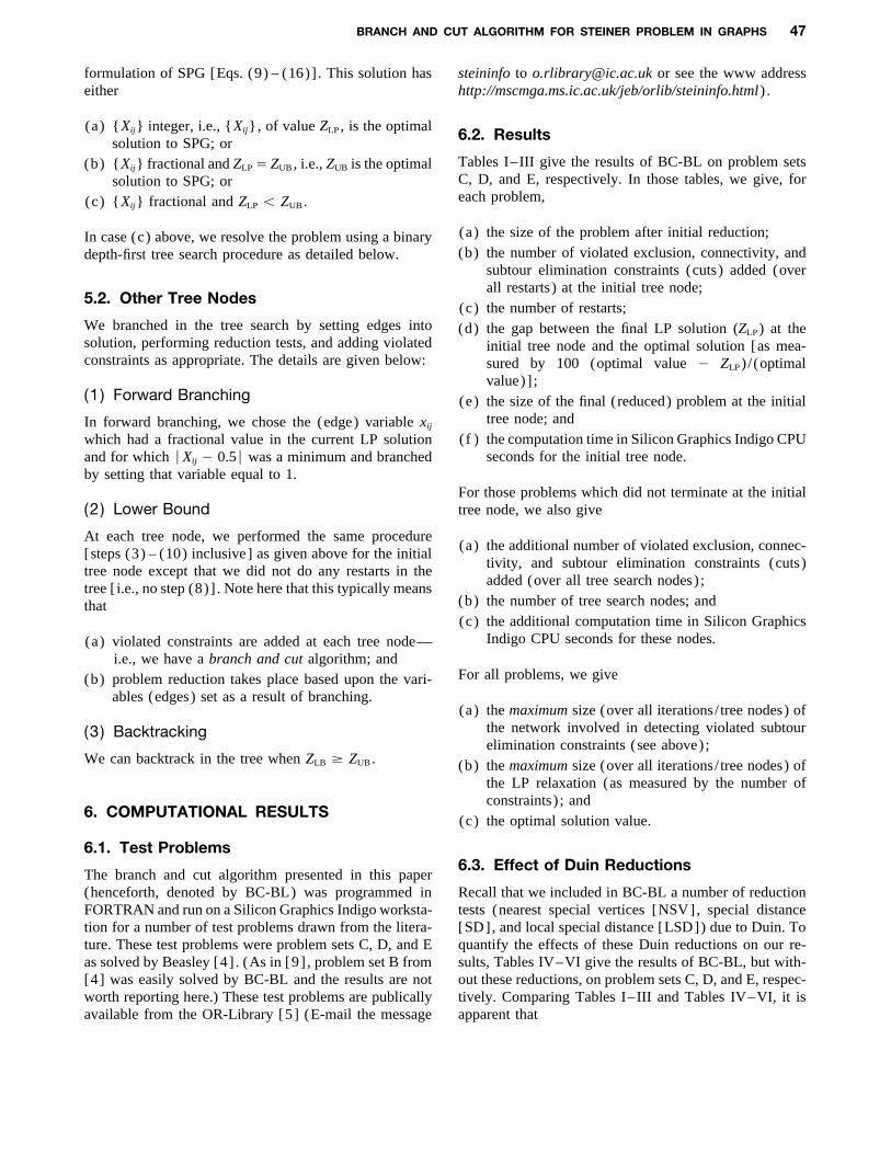
formulation of SPG [Eqs. (9) – (16)] . This solution has steininfo to [email protected] or see the www addresshttp://mscmga.ms.ic.ac.uk/jeb/orlib/steininfo.html) .either
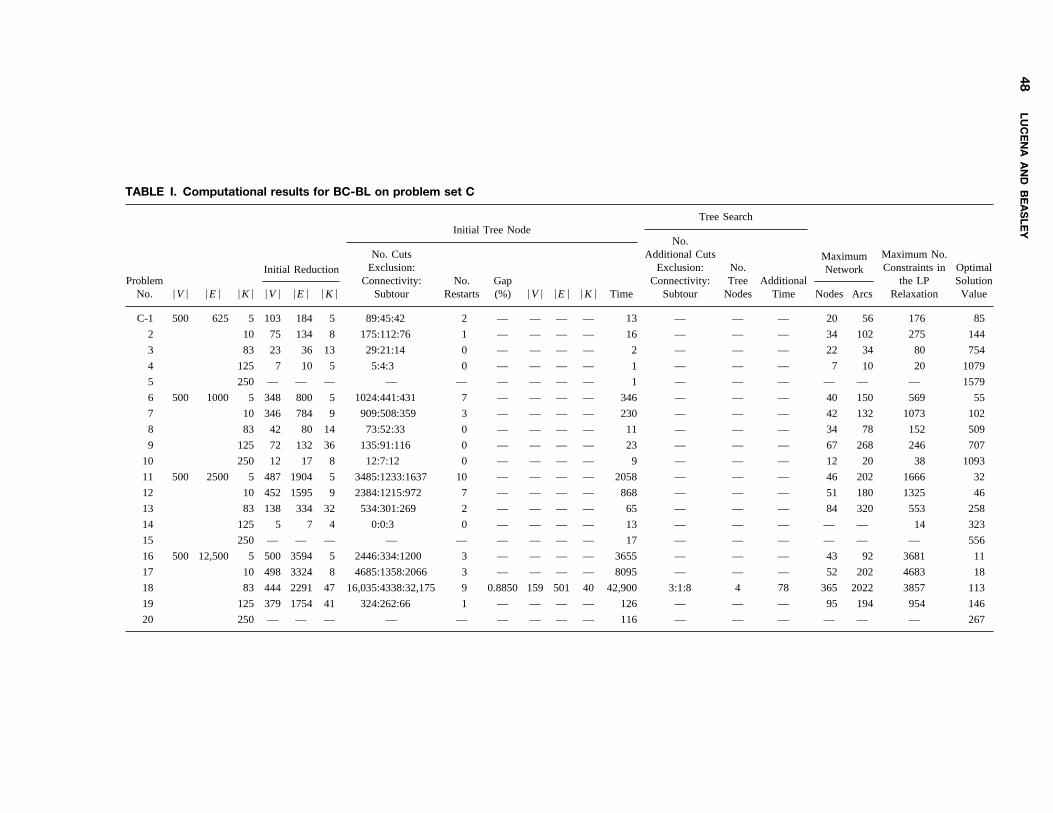
(a) {Xij} integer, i.e., {Xij}, of value ZLP , is the optimal 6.2. Resultssolution to SPG; orTables I–III give the results of BC-BL on problem sets(b) {Xij} fractional and ZLPÅ ZUB, i.e., ZUB is the optimalC, D, and E, respectively. In those tables, we give, forsolution to SPG; oreach problem,(c) {Xij} fractional and ZLP õ ZUB.
(a) the size of the problem after initial reduction;In case (c) above, we resolve the problem using a binary(b) the number of violated exclusion, connectivity, anddepth-first tree search procedure as detailed below.
subtour elimination constraints (cuts) added (overall restarts) at the initial tree node;
5.2. Other Tree Nodes(c) the number of restarts;
We branched in the tree search by setting edges into (d) the gap between the final LP solution (ZLP) at thesolution, performing reduction tests, and adding violated initial tree node and the optimal solution [as mea-constraints as appropriate. The details are given below: sured by 100 (optimal value 0 ZLP) /(optimal
value)] ;(1 ) Forward Branching (e) the size of the final (reduced) problem at the initial
tree node; andIn forward branching, we chose the (edge) variable xij
(f ) the computation time in Silicon Graphics Indigo CPUwhich had a fractional value in the current LP solutionseconds for the initial tree node.and for which ÉXij 0 0.5É was a minimum and branched
by setting that variable equal to 1.For those problems which did not terminate at the initialtree node, we also give(2 ) Lower Bound
At each tree node, we performed the same procedure(a) the additional number of violated exclusion, connec-[steps (3) – (10) inclusive] as given above for the initial
tivity, and subtour elimination constraints (cuts)tree node except that we did not do any restarts in theadded (over all tree search nodes);tree [i.e., no step (8)] . Note here that this typically means
(b) the number of tree search nodes; andthat(c) the additional computation time in Silicon Graphics
Indigo CPU seconds for these nodes.(a) violated constraints are added at each tree node—i.e., we have a branch and cut algorithm; and
For all problems, we give(b) problem reduction takes place based upon the vari-ables (edges) set as a result of branching.
(a) the maximum size (over all iterations/ tree nodes) ofthe network involved in detecting violated subtour(3 ) Backtrackingelimination constraints (see above);
We can backtrack in the tree when ZLB ¢ ZUB. (b) the maximum size (over all iterations/ tree nodes) ofthe LP relaxation (as measured by the number ofconstraints) ; and
6. COMPUTATIONAL RESULTS(c) the optimal solution value.
6.1. Test Problems6.3. Effect of Duin Reductions
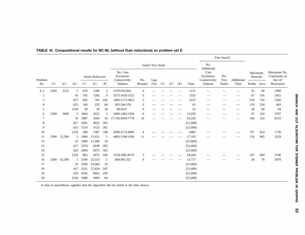
The branch and cut algorithm presented in this paper(henceforth, denoted by BC-BL) was programmed in Recall that we included in BC-BL a number of reduction
tests (nearest special vertices [NSV], special distanceFORTRAN and run on a Silicon Graphics Indigo worksta-tion for a number of test problems drawn from the litera- [SD], and local special distance [LSD]) due to Duin. To
quantify the effects of these Duin reductions on our re-ture. These test problems were problem sets C, D, and Eas solved by Beasley [4] . (As in [9] , problem set B from sults, Tables IV–VI give the results of BC-BL, but with-
out these reductions, on problem sets C, D, and E, respec-[4] was easily solved by BC-BL and the results are notworth reporting here.) These test problems are publically tively. Comparing Tables I–III and Tables IV–VI, it is
apparent thatavailable from the OR-Library [5] (E-mail the message
8U1D 793/ 8U1D$$0793 11-11-97 09:14:01 netwa W: Networks
48LU
CE
NA
AN
DB
EA
SLE
Y
TABLE I. Computational results for BC-BL on problem set C
Tree SearchInitial Tree Node
No.No. Cuts Additional Cuts Maximum No.Maximum
Exclusion: Exclusion: No. Constraints in OptimalInitial Reduction NetworkProblem Connectivity: No. Gap Connectivity: Tree Additional the LP Solution
No. ÉVÉ ÉEÉ ÉKÉ ÉVÉ ÉEÉ ÉKÉ Subtour Restarts (%) ÉVÉ ÉEÉ ÉKÉ Time Subtour Nodes Time Nodes Arcs Relaxation Value
C-1 500 625 5 103 184 5 89:45:42 2 — — — — 13 — — — 20 56 176 85
2 10 75 134 8 175:112:76 1 — — — — 16 — — — 34 102 275 144
3 83 23 36 13 29:21:14 0 — — — — 2 — — — 22 34 80 754
4 125 7 10 5 5:4:3 0 — — — — 1 — — — 7 10 20 1079
5 250 — — — — — — — — — 1 — — — — — — 1579
6 500 1000 5 348 800 5 1024:441:431 7 — — — — 346 — — — 40 150 569 55
7 10 346 784 9 909:508:359 3 — — — — 230 — — — 42 132 1073 102
8 83 42 80 14 73:52:33 0 — — — — 11 — — — 34 78 152 509
9 125 72 132 36 135:91:116 0 — — — — 23 — — — 67 268 246 707
10 250 12 17 8 12:7:12 0 — — — — 9 — — — 12 20 38 1093
11 500 2500 5 487 1904 5 3485:1233:1637 10 — — — — 2058 — — — 46 202 1666 32
12 10 452 1595 9 2384:1215:972 7 — — — — 868 — — — 51 180 1325 46
13 83 138 334 32 534:301:269 2 — — — — 65 — — — 84 320 553 258
14 125 5 7 4 0:0:3 0 — — — — 13 — — — — — 14 323
15 250 — — — — — — — — — 17 — — — — — — 556
16 500 12,500 5 500 3594 5 2446:334:1200 3 — — — — 3655 — — — 43 92 3681 11
17 10 498 3324 8 4685:1358:2066 3 — — — — 8095 — — — 52 202 4683 18
18 83 444 2291 47 16,035:4338:32,175 9 0.8850 159 501 40 42,900 3:1:8 4 78 365 2022 3857 113
19 125 379 1754 41 324:262:66 1 — — — — 126 — — — 95 194 954 146
20 250 — — — — — — — — — 116 — — — — — — 267
8U1D
793/8U
1D$$0793
11-11-9709:14:01
netwa
W:
Netw
orks

BR
AN
CH
AN
DC
UT
ALG
OR
ITH
MFO
RS
TE
INE
RP
RO
BLE
MIN
GR
AP
HS
49
TABLE II. Computational results for BC-BL on problem set D
Tree SearchInitial Tree Node
No. MaximumNo. Cuts Additional Cuts No.Maximum
Exclusion: Exclusion: No. Constraints OptimalInitial Reduction NetworkProblem Connectivity: No. Gap Connectivity: Tree Additional in the LP Solution
No. ÉVÉ ÉEÉ ÉKÉ ÉVÉ ÉEÉ ÉKÉ Subtour Restarts (%) ÉVÉ ÉEÉ ÉKÉ Time Subtour Nodes Time Nodes Arcs Relaxation Value
D-1 1000 1250 5 226 424 5 432:227:177 3 — — — — 106 — — — 31 94 376 106
2 10 247 454 10 530:225:184 2 — — — — 77 — — — 61 210 580 220
3 167 — — — — — — — — — 5 — — — — — — 1565
4 250 13 18 8 11:9:6 0 — — — — 5 — — — 13 20 38 1935
5 500 8 12 6 6:2:1 0 — — — — 8 — — — 8 28 19 3250
6 1000 2000 5 737 1694 5 2867:1401:1125 6 5.7836 107 298 5 2088 254:70:157 12 103 85 532 1432 67
7 10 711 1634 10 1618:568:667 3 — — — — 744 — — — 47 136 1718 103
8 167 103 178 47 186:118:151 0 — — — — 90 — — — 97 352 333 1072
9 250 7 10 5 5:3:1 0 — — — — 71 — — — 7 18 18 1448
10 500 15 28 11 11:5:9 0 — — — — 52 — — — 15 26 37 2110
11 1000 5000 5 975 4190 5 6303:1198:2847 11 — — — — 8076 — — — 84 484 2764 29
12 10 950 3568 9 4353:1382:1665 7 2.3810 11 26 5 3446 1:1:0 2 1 66 346 2265 42
13 167 12 20 7 14:9:8 0 — — — — 111 — — — 11 20 40 500
14 250 — — — — — — — — — 110 — — — — — — 667
15 500 8 13 6 4:2:0 0 — — — — 114 — — — 8 10 17 1116
16 1000 25,000 5 1000 8296 5 466:270:198 3 — — — — 1200 — — — 24 70 1276 13
17 10 999 7997 9 5111:392:2412 1 — — — — 17,856 — — — 71 158 8181 23
18 167 896 4737 94 12,115:4124:9654 2 — — — — 14,968 — — — 768 4328 7806 223
19 250 801 4112 97 3802:1289:2344 0 — — — — 20,893 — — — 342 1666 6669 310
20 500 — — — — — — — — — 791 — — — — — — 537
8U1D
793/8U
1D$$0793
11-11-9709:14:01
netwa
W:
Netw
orks

50LU
CE
NA
AN
DB
EA
SLE
Y
TABLE III. Computational results for BC-BL on problem set E
Tree Search
No.Initial Tree NodeAdditional
No. Cuts Cuts Maximum No.MaximumExclusion: Exclusion: No. Constraints in OptimalInitial Reduction Network
Problem Connectivity: No. Gap Connectivity: Tree Additional the LP SolutionNo. ÉVÉ ÉEÉ ÉKÉ ÉVÉ ÉEÉ ÉKÉ Subtour Restarts (%) ÉVÉ ÉEÉ ÉKÉ Time Subtour Nodes Time Nodes Arcs Relaxation Value
E-1 2500 3125 5 647 1234 5 1357:295:650 5 — — — — 1028 — — — 30 68 1716 111
2 10 666 1244 9 3079:1525:1295 4 — — — — 1765 — — — 64 310 2530 214
3 417 81 135 46 115:77:120 0 — — — — 113 — — — 79 222 248 4013
4 625 19 33 13 17:9:6 0 — — — — 75 — — — 19 34 48 5101
5 1250 7 10 5 5:4:3 0 — — — — 99 — — — 7 10 19 8128
6 2500 5000 5 1816 4268 5 8846:2028:4179 8 — — — — 8547 — — — 51 168 5792 73
7 10 1861 4322 10 17,461:4000:1107 8 0.3448 341 652 10 11,801 1:1:0 4 52 492 1630 8430 145
8 417 188 349 90 371:234:470 0 — — — — 1204 — — — 171 464 642 2640
9 625 78 136 42 94:61:35 0 — — — — 1083 — — — 72 152 193 3604
10 1250 11 18 8 10:4:4 0 — — — — 814 — — — 11 20 28 5600
11 2500 12,500 5 2479 11,479 5 2350:1337:757 8 — — — — 10,426 — — — 56 268 3005 34
12 10 2455 10,834 10 (21,600)
13 417 300 655 116 2041:890:3517 2 — — — — 7484 — — — 280 1128 1128 1280
14 625 34 61 19 45:33:22 0 — — — — 1806 — — — 33 68 113 1732
15 1250 — — — — — — — — — 1599 — — — — — — 2784
16 2500 62,500 5 2500 23,397 5 1192:639:448 4 — — — — 13,517 — — — 34 98 3524 15
17 10 2500 21,783 10 (21,600)
18 417 2259 12,255 247 (21,600)
19 625 1777 8173 183 (21,600)
20 1250 — — — — — — — — — 10,277 — — — — — — 1342
A time in parentheses signifies that the algorithm did not finish in the time shown.
8U1D
793/8U
1D$$0793
11-11-9709:14:01
netwa
W:
Netw
orks

BR
AN
CH
AN
DC
UT
ALG
OR
ITH
MFO
RS
TE
INE
RP
RO
BLE
MIN
GR
AP
HS
51
TABLE IV. Computational results for BC-BL (without Duin reductions) on problem set C
Tree SearchInitial Tree Node
No.No. Cuts Additional Cuts Maximum No.Maximum
Exclusion: Exclusion: No. Constraints inInitial Reduction NetworkProblem Connectivity: No. Gap Connectivity: Tree Additional the LP
No. ÉVÉ ÉEÉ ÉKÉ ÉVÉ ÉEÉ ÉKÉ Subtour Restarts (%) ÉVÉ ÉEÉ ÉKÉ Time Subtour Nodes Time Nodes Arcs Relaxation
C-1 500 625 5 138 241 5 172:100:91 3 — — — — 16 — — — 23 56 220
2 10 128 228 8 465:289:219 5 — — — — 34 — — — 34 108 423
3 83 103 162 31 276:155:125 3 — — — — 12 — — — 69 150 319
4 125 87 132 30 204:135:96 1 — — — — 10 — — — 63 128 273
5 250 18 23 11 15:7:7 0 — — — — 1 — — — 16 20 47
6 500 1000 5 366 830 5 1637:679:755 9 — — — — 352 — — — 61 196 605
7 10 381 848 9 1326:825:515 4 — — — — 270 — — — 45 162 997
8 83 342 731 53 2148:1071:1125 6 — — — — 273 — — — 146 338 1215
9 125 317 644 68 2476:1182:2144 3 0.2829 178 395 63 1052 209:140:678 66 1153 170 714 1080
10 250 51 77 22 53:32:20 0 — — — — 7 — — — 39 62 141
11 500 2500 5 500 1967 5 2239:761:1176 10 — — — — 1789 — — — 56 172 1742
12 10 497 1856 9 3377:1549:1381 10 — — — — 1065 — — — 50 172 1307
13 83 425 1301 48 2517:1091:1409 3 0.7623 173 475 41 761 328:382:749 50 1841 146 754 1421
14 125 383 1068 62 966:500:544 1 — — — — 131 — — — 152 386 1309
15 250 85 158 22 145:121:59 2 — — — — 21 — — — 48 138 232
16 500 12,500 5 500 3661 5 144:108:83 2 — — — — 174 — — — 17 40 592
17 10 498 3535 8 2390:417:1097 1 — — — — 3039 — — — 57 116 4095
18 83 463 2718 47 21,486:5844:33,229 17 0.8850 59 101 30 30,344 0:0:0 4 31 371 2014 3699
19 125 416 1952 41 571:451:176 2 — — — — 130 — — — 89 152 1000
20 250 190 521 10 63:56:16 0 — — — — 142 — — — 23 38 314
8U1D
793/8U
1D$$0793
11-11-9709:14:01
netwa
W:
Netw
orks

52LU
CE
NA
AN
DB
EA
SLE
Y
TABLE V. Computational results for BC-BL (without Duin reductions) on problem set D
Tree Search
No.Initial Tree NodeAdditional
No. Cuts Cuts Maximum No.MaximumExclusion: Exclusion: No. Constraints inInitial Reduction Network
Problem Connectivity: No. Gap Connectivity: Tree Additional the LPNo. ÉVÉ ÉEÉ ÉKÉ ÉVÉ ÉEÉ ÉKÉ Subtour Restarts (%) ÉVÉ ÉEÉ ÉKÉ Time Subtour Nodes Time Nodes Arcs Relaxation
D-1 1000 1250 5 276 508 5 858:530:361 9 3.7736 14 26 5 142 13:12:5 8 2 33 112 499
2 10 287 518 10 647:274:224 2 — — — — 81 — — — 69 282 687
3 167 177 273 54 363:241:150 2 — — — — 21 — — — 116 208 539
4 250 99 144 41 140:72:70 0 — — — — 12 — — — 78 200 298
5 500 48 62 26 58:42:163 0 — — — — 29 — — — 45 142 193
6 1000 2000 5 759 1727 5 2994:1431:1181 7 5.2239 101 272 5 1558 140:59:139 8 54 80 380 1352
7 10 747 1700 10 1595:589:645 3 — — — — 620 — — — 49 148 1811
8 167 707 1501 113 3636:2025:2089 4 — — — — 717 — — — 319 710 2395
9 250 613 1294 136 4299:2501:3094 8 — — — — 1219 — — — 326 816 2036
10 500 294 623 92 1021:651:903 4 — — — — 190 — — — 177 370 830
11 1000 5000 5 992 4297 5 6295:1452:3035 12 — — — — 5943 — — — 53 128 3016
12 10 995 4031 9 3245:954:1347 8 2.3810 8 12 4 2316 1:1:0 2 1 67 352 2816
13 167 891 2855 108 7620:4176:4892 8 — — — — 2107 — — — 297 792 2959
14 250 759 2141 115 6341:3460:4293 6 — — — — 1554 — — — 289 634 2640
15 500 210 425 56 731:410:315 3 — — — — 149 — — — 117 222 690
16 1000 25,000 5 1000 8338 5 509:348:249 4 — — — — 1128 — — — 24 82 1267
17 10 999 8308 9 5315:580:2852 2 — — — — 16,928 — — — 745 3964 8168
18 167 927 5948 94 13,951:3598:10,582 2 — — — — 15,223 — — — 787 4486 7406
19 250 841 4559 97 4477:1205:6013 0 — — — — 9020 — — — 685 4054 6397
20 500 418 1142 33 218:168:49 0 — — — — 905 — — — 80 154 828
8U1D
793/8U
1D$$0793
11-11-9709:14:01
netwa
W:
Netw
orks
BR
AN
CH
AN
DC
UT
ALG
OR
ITH
MFO
RS
TE
INE
RP
RO
BLE
MIN
GR
AP
HS
53
TABLE VI. Computational results for BC-BL (without Duin reductions) on problem set E
Tree Search
No.Initial Tree NodeAdditional
No. Cuts Cuts Maximum No.MaximumExclusion: Exclusion: No. Constraints inInitial Reduction Network
Problem Connectivity: No. Gap Connectivity: Tree Additional the LPNo. ÉVÉ ÉEÉ ÉKÉ ÉVÉ ÉEÉ ÉKÉ Subtour Restarts (%) ÉVÉ ÉEÉ ÉKÉ Time Subtour Nodes Time Nodes Arcs Relaxation
E-1 2500 3125 5 678 1280 5 1978:453:956 6 — — — — 1131 — — — 35 90 1990
2 10 705 1305 9 3575:1618:1522 5 — — — — 1555 — — — 67 316 2452
3 417 492 781 145 1900:1173:3853 2 — — — — 2147 — — — 310 716 1565
4 625 160 225 64 385:244:150 2 — — — — 61 — — — 119 224 463
5 1250 30 30 18 28:20:9 0 — — — — 55 — — — 28 68 84
6 2500 5000 5 1844 4331 5 5490:1402:2594 6 — — — — 13,050 — — — 47 162 5707
7 10 1887 4344 10 17,730:4930:7778 14 — — — — 10,243 — — — 106 234 8133
8 417 1691 4022 265 (21,600)
9 625 1514 3723 301 (21,600)
10 1250 584 1387 188 2698:2174:4906 4 — — — — 4483 — — — 357 814 1736
11 2500 12,500 5 2498 11,631 5 4863:2190:1436 11 — — — — 17,103 — — — 154 902 3529
12 10 2498 11,500 10 (21,600)
13 417 2274 8249 282 (21,600)
14 625 2004 6973 302 (21,600)
15 1250 802 2073 166 3159:1981:8570 5 — — — — 10,294 — — — 327 904 3746
16 2500 62,500 5 2500 23,553 5 684:485:322 4 — — — — 13,717 — — — 28 76 2878
17 10 2500 23,064 10 (21,600)
18 417 2321 17,634 247 (21,600)
19 625 2042 9663 190 (21,600)
20 1250 1088 3084 84 (21,600)
A time in parentheses signifies that the algorithm did not finish in the time shown.
8U1D
793/8U
1D$$0793
11-11-9709:14:01
netwa
W:
Netw
orks
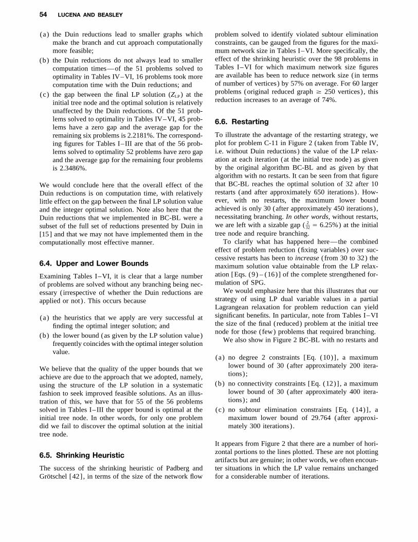
54 LUCENA AND BEASLEY
(a) the Duin reductions lead to smaller graphs which problem solved to identify violated subtour eliminationconstraints, can be gauged from the figures for the maxi-make the branch and cut approach computationally
more feasible; mum network size in Tables I–VI. More specifically, theeffect of the shrinking heuristic over the 98 problems in(b) the Duin reductions do not always lead to smallerTables I–VI for which maximum network size figurescomputation times—of the 51 problems solved toare available has been to reduce network size (in termsoptimality in Tables IV–VI, 16 problems took moreof number of vertices) by 57% on average. For 60 largercomputation time with the Duin reductions; andproblems (original reduced graph ¢ 250 vertices) , this(c) the gap between the final LP solution (ZLP) at thereduction increases to an average of 74%.initial tree node and the optimal solution is relatively
unaffected by the Duin reductions. Of the 51 prob-lems solved to optimality in Tables IV–VI, 45 prob- 6.6. Restartinglems have a zero gap and the average gap for the
To illustrate the advantage of the restarting strategy, weremaining six problems is 2.2181%. The correspond-plot for problem C-11 in Figure 2 (taken from Table IV,ing figures for Tables I–III are that of the 56 prob-i.e. without Duin reductions) the value of the LP relax-lems solved to optimality 52 problems have zero gapation at each iteration (at the initial tree node) as givenand the average gap for the remaining four problemsby the original algorithm BC-BL and as given by thatis 2.3486%.algorithm with no restarts. It can be seen from that figurethat BC-BL reaches the optimal solution of 32 after 10We would conclude here that the overall effect of therestarts (and after approximately 650 iterations) . How-Duin reductions is on computation time, with relativelyever, with no restarts, the maximum lower boundlittle effect on the gap between the final LP solution valueachieved is only 30 (after approximately 450 iterations) ,and the integer optimal solution. Note also here that thenecessitating branching. In other words, without restarts,Duin reductions that we implemented in BC-BL were awe are left with a sizable gap ( 2
32 Å 6.25%) at the initialsubset of the full set of reductions presented by Duin intree node and require branching.[15] and that we may not have implemented them in the
To clarify what has happened here—the combinedcomputationally most effective manner.effect of problem reduction (fixing variables) over suc-cessive restarts has been to increase (from 30 to 32) the
6.4. Upper and Lower Bounds maximum solution value obtainable from the LP relax-ation [Eqs. (9) – (16)] of the complete strengthened for-Examining Tables I–VI, it is clear that a large numbermulation of SPG.of problems are solved without any branching being nec-
We would emphasize here that this illustrates that ouressary (irrespective of whether the Duin reductions arestrategy of using LP dual variable values in a partialapplied or not) . This occurs becauseLagrangean relaxation for problem reduction can yieldsignificant benefits. In particular, note from Tables I–VI(a) the heuristics that we apply are very successful atthe size of the final (reduced) problem at the initial treefinding the optimal integer solution; andnode for those (few) problems that required branching.(b) the lower bound (as given by the LP solution value)
We also show in Figure 2 BC-BL with no restarts andfrequently coincides with the optimal integer solutionvalue.
(a) no degree 2 constraints [Eq. (10)] , a maximumlower bound of 30 (after approximately 200 itera-We believe that the quality of the upper bounds that wetions);achieve are due to the approach that we adopted, namely,
(b) no connectivity constraints [Eq. (12)] , a maximumusing the structure of the LP solution in a systematiclower bound of 30 (after approximately 400 itera-fashion to seek improved feasible solutions. As an illus-tions); andtration of this, we have that for 55 of the 56 problems
(c) no subtour elimination constraints [Eq. (14)] , asolved in Tables I–III the upper bound is optimal at themaximum lower bound of 29.764 (after approxi-initial tree node. In other words, for only one problemmately 300 iterations) .did we fail to discover the optimal solution at the initial
tree node.It appears from Figure 2 that there are a number of hori-zontal portions to the lines plotted. These are not plotting6.5. Shrinking Heuristicartifacts but are genuine; in other words, we often encoun-ter situations in which the LP value remains unchangedThe success of the shrinking heuristic of Padberg and
Grotschel [42], in terms of the size of the network flow for a considerable number of iterations.
8U1D 793/ 8U1D$$0793 11-11-97 09:14:01 netwa W: Networks

BRANCH AND CUT ALGORITHM FOR STEINER PROBLEM IN GRAPHS 55
Fig. 2. Problem C-11.
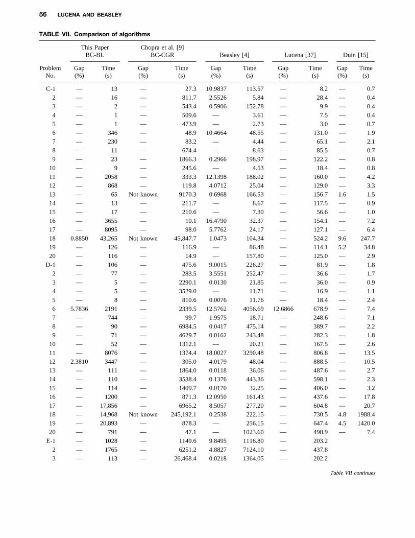
6.7. Comparison rior, not only in computation time terms but also ingap terms, to the Lagrangean relaxation algorithm of
In Table VII, we compare BC-BL (with Duin reductions, Beasley [4]; andTables I–III) with the results of other workers. In that
(c) although the performance of Duin [15] on problemtable, we present the gap at the initial tree node (if known)set E is unknown, it is clear that its computationand the total computation time in seconds. However, allperformance on problems sets C and D is superiorthe computers used were different, which makes a preciseto all other algorithms.comparison of these results difficult. Chopra et al. [9] in
their branch and cut algorithm (henceforth, denoted byBC-CGR) used a Vax 8700; Beasley [4] , a Cray X-MP/ 6.8. Duin [15] Results48; Lucena [37], a Sun Sparcstation 10; and Duin [15],
The performance of Duin [15] deserves further comment.a 486 66 MHz pc.We believe that the key to his success is twofold:From Dongarra [13], we can make an approximate
comparison of the results shown in Table VII by usingscaling values for the achievable speeds of these comput- 1. His reduction tests are very effective.ers as 15 for the Silicon Graphics Indigo, 0.99 for the 2. His computational implementation is outstandingly ef-Vax 8700, 121 for the Cray X-MP/48, 7 for the Sun fective.Sparcstation 10, and 0.56 for the 486 66 MHz pc. Usingthese values, we would make the following observations: In support of this, we would note that BC-BL includes a
subset of the full set of Duin reductions [15], yet it is(a) Among BC-BL, BC-CGR, and Lucena, no clear clear from the comparable problems solved by BC-BL
computational winner emerges: BC-BL is faster than purely by reduction (problems C-5/15/20, D-3/14/20)BC-CGR in solving 26 problems, BC-BL is faster that our computation times are far inferior to those ofthan Lucena in solving 23 problems, and Lucena is Duin. Indeed, for these particular problems, our total com-faster than BC-CGR in solving 28 problems; putation time is 1040 Silicon Graphics Indigo seconds
while the computation time for Duin for these problems(b) BC-BL, BC-CGR, and Lucena are all generally supe-
8U1D 793/ 8U1D$$0793 11-11-97 09:14:01 netwa W: Networks
56 LUCENA AND BEASLEY
TABLE VII. Comparison of algorithms
This Paper Chopra et al. [9]BC-BL BC-CGR Beasley [4] Lucena [37] Duin [15]
Problem Gap Time Gap Time Gap Time Gap Time Gap TimeNo. (%) (s) (%) (s) (%) (s) (%) (s) (%) (s)
C-1 — 13 — 27.3 10.9837 113.57 — 8.2 — 0.7
2 — 16 — 811.7 2.5526 5.84 — 28.4 — 0.4
3 — 2 — 543.4 0.5906 152.78 — 9.9 — 0.4
4 — 1 — 509.6 — 3.61 — 7.5 — 0.4
5 — 1 — 473.9 — 2.73 — 3.0 — 0.7
6 — 346 — 48.9 10.4664 48.55 — 131.0 — 1.9
7 — 230 — 83.2 — 4.44 — 65.1 — 2.1
8 — 11 — 674.4 — 8.63 — 85.5 — 0.7
9 — 23 — 1866.3 0.2966 198.97 — 122.2 — 0.8
10 — 9 — 245.6 — 4.53 — 18.4 — 0.8
11 — 2058 — 333.3 12.1398 188.02 — 160.0 — 4.2
12 — 868 — 119.8 4.0712 25.04 — 129.0 — 3.3
13 — 65 Not known 9170.3 0.6968 166.53 — 156.7 1.6 1.5
14 — 13 — 211.7 — 8.67 — 117.5 — 0.9
15 — 17 — 210.6 — 7.30 — 56.6 — 1.0
16 — 3655 — 10.1 16.4790 32.37 — 154.1 — 7.2
17 — 8095 — 98.0 5.7762 24.17 — 127.1 — 6.4
18 0.8850 43,265 Not known 45,847.7 1.0473 104.34 — 524.2 9.6 247.7
19 — 126 — 116.9 — 86.48 — 114.1 5.2 34.8
20 — 116 — 14.9 — 157.80 — 125.0 — 2.9
D-1 — 106 — 475.6 9.0015 226.27 — 81.9 — 1.8
2 — 77 — 283.5 3.5551 252.47 — 36.6 — 1.7
3 — 5 — 2290.1 0.0130 21.85 — 36.0 — 0.9
4 — 5 — 3529.0 — 11.71 — 16.9 — 1.1
5 — 8 — 810.6 0.0076 11.76 — 18.4 — 2.4
6 5.7836 2191 — 2339.5 12.5762 4056.69 12.6866 678.9 — 7.4
7 — 744 — 99.7 1.9575 18.71 — 248.6 — 7.1
8 — 90 — 6984.5 0.0417 475.14 — 389.7 — 2.2
9 — 71 — 4629.7 0.0162 243.48 — 282.3 — 1.8
10 — 52 — 1312.1 — 20.21 — 167.5 — 2.6
11 — 8076 — 1374.4 18.0027 3290.48 — 806.8 — 13.5
12 2.3810 3447 — 305.0 4.0179 48.04 — 888.5 — 10.5
13 — 111 — 1864.0 0.0118 36.06 — 487.6 — 2.7
14 — 110 — 3538.4 0.1376 443.36 — 598.1 — 2.3
15 — 114 — 1409.7 0.0170 32.25 — 406.0 — 3.2
16 — 1200 — 871.3 12.0950 161.43 — 437.6 — 17.8
17 — 17,856 — 6965.2 8.5057 277.20 — 604.8 — 20.7
18 — 14,968 Not known 245,192.1 0.2538 222.15 — 730.5 4.8 1988.4
19 — 20,893 — 878.3 — 256.15 — 647.4 4.5 1420.0
20 — 791 — 47.1 — 1023.60 — 498.9 — 7.4
E-1 — 1028 — 1149.6 9.8495 1116.80 — 203.2
2 — 1765 — 6251.2 4.8827 7124.10 — 437.8
3 — 113 — 26,468.4 0.0218 1364.05 — 202.2
Table VII continues
8U1D 793/ 8U1D$$0793 11-11-97 09:14:01 netwa W: Networks

BRANCH AND CUT ALGORITHM FOR STEINER PROBLEM IN GRAPHS 57
TABLE VII. Continued
This Paper Chopra et al. [9]BC-BL BC-CGR Beasley [4] Lucena [37] Duin [15]
Problem Gap Time Gap Time Gap Time Gap Time Gap TimeNo. (%) (s) (%) (s) (%) (s) (%) (s) (%) (s)
4 — 75 — 46,007.6 0.0339 378.66 — 206.7
5 — 99 — 12,564.1 — 98.22 — 215.1
6 — 8547 — 678.0 10.5719 1760.49 — 2860.0
7 0.3448 11,853 — 27,124.0 14.0949 (21,600) — 2852.2
8 — 1204 — 118,617.5 0.0246 4459.30 — 3198.4
9 — 1083 — 24,527.8 0.0434 18,818.53 — 2235.5
10 — 814 — 39,260.7 0.0161 311.87 — 1797.1
11 — 10,426 — 1900.6 9.9758 3061.45 — 5319.0
12 (21,600) — 7199.7 9.4853 (21,600) — 6159.8
13 — 7484 — 207,058.6 0.9272 (21,600) — 9311.9
14 — 1806 — 29,262.6 0.2527 (21,600) — 6729.6
15 — 1599 — 7666.0 0.0161 457.98 — 4611.8
16 — 13,517 — 179.0 16.0455 7880.44 — 3570.4
17 (21,600) — 36,039.9 4.6859 445.69 — 4729.7
18 (21,600) Not known Not known 16.3308 (21,600) 0.8979 (50,000)
19 (21,600) — 6371.8 0.5759 (21,600) — 18,345.0
20 — 10,277 — 272.2 — 14,037.13 — 15,832.5
is 15.2 486 66 MHz pc seconds. Given the Dongarra [13] • using LP dual variable values in a partial Lagrangeanrelaxation,scaling factors of 15 and 0.56, respectively, these times
equate to a ratio of 1040(15):15.2(0.56) Å 1833:1, i.e., • using the structure of the LP solution to look for feasi-our best estimate is that our implementation is at least ble solutions, andthree orders of magnitude slower than the implementation • restartingof Duin.
We would also comment that our experimental evi-relating to branch and cut algorithms in general weredence (presented above) has been that the effect of thehighlighted.subset of the full set of Duin reductions [15] incorporated
into BC-BL is principally upon the computation time andnot on the gap between the final LP solution value andthe integer optimal solution. In particular, note that the REFERENCESgaps found by BC-BL are much smaller than are the gapsreported by Duin using a lower bound due to Wong [57],
[1] Y. P. Aneja, An integer linear programming approach towhich from Table VII average to a gap figure of 0.6425%the Steiner problem in graphs. Networks 10 (1980) 167–over the 40 problems in problem sets C and D. This178.compares with an average for BC-BL of 0.2262% and an
[ 2] A. Balakrishnan and N. R. Patel, Problem reductionaverage for Lucena of 0.3172%.methods and a tree generation algorithm for the Steinernetwork problem. Networks 17 (1987) 65–85.
[ 3] J. E. Beasley, An algorithm for the Steiner problem in7. CONCLUSIONS graphs. Networks 14 (1984) 147–159.
[ 4] J. E. Beasley, An SST-based algorithm for the Steinerproblem in graphs. Networks 19 (1989) 1–16.In this paper, we have presented a branch and cut algo-
rithm for the Steiner problem in graphs. Computational [ 5] J. E. Beasley, OR-Library: Distributing test problems byelectronic mail. J. Oper. Res. Soc. 41 (1990) 1069–results indicated that the algorithm developed is able to1072.solve a large number of problems without resorting to
[ 6] J. E. Beasley, Lagrangean relaxation. Modern Heuristicbranching. In addition, a number of issues, specifically,
8U1D 793/ 8U1D$$0793 11-11-97 09:14:01 netwa W: Networks
58 LUCENA AND BEASLEY
Techniques for Combinatorial Problems (C. R. Reeves, solving integer programming problems. Manag. Sci. 27(1981) 1–18.Ed.) . Blackwell, Oxford (1993) 243–303.
[ 24] M. L. Fisher, An applications oriented guide to Lagran-[ 7] P. Berman and V. Ramaiyer, Improved approximations forgian relaxation. Interfaces 15 (1985) 10–21.the Steiner tree problem. J. Alg. 17 (1994) 381–408.
[ 25] R. Floren, A note on ‘‘A faster approximation algorithm[ 8] S. Chopra and E. R. Gorres, On the node weightedfor the Steiner problem in graphs.’’ Inform. Process.Steiner tree problem. Working paper. Available from theLett. 38 (1991) 177–178.first author at Department of Managerial Economics and
Decision Sciences, J. L. Kellogg Graduate School of [ 26] M. X. Goemans and Y. Myung, A catalog of SteinerManagement, Northwestern University, Evanston IL tree formulations. Networks 23 (1993) 19–28.60208 (1990).
[ 27] D. Goldfarb and M. D. Grigoriadis, A computational[ 9] S. Chopra, E. R. Gorres, and M. R. Rao, Solving the comparison of the Dinic and network simplex methods
Steiner tree problem on a graph using branch and cut. for maximum flow. Ann. Oper. Res. 13 (1988) 83–123.ORSA J. Comput. 4 (1992) 320–335. [ 28] F. K. Hwang and D. S. Richards, Steiner tree problems.
[10] S. Chopra and M. R. Rao, The Steiner tree problem I: Networks 22 (1992) 55–89.Formulations, compositions and extension of facets. [ 29] F. K. Hwang, D. S. Richards, and P. Winter, The SteinerMath. Prog. 64 (1994) 209–229. Tree Problem. North-Holland, Amsterdam (1992).
[11] S. Chopra and M. R. Rao, The Steiner tree problem II: [ 30] A. Kapsalis, V. J. Rayward-Smith, and G. D. Smith,Properties and classes of facets. Math. Prog. 64 (1994) Solving the graphical Steiner tree problem using genetic231–246. algorithms. J. Oper. Res. Soc. 44 (1993) 397–406.
[12] CPLEX Optimization Inc., Using the CPLEX Callable [ 31] B. N. Khoury and P. M. Pardalos, A heuristic for theLibrary. CPLEX Optimization Inc., Suite 279, 930 Ta- Steiner problem in graphs. Working paper. Availablehoe Blvd., Bldg. 802, Incline Valley, NV 89451-9436 from the authors at Department of Industrial and Systems(1995). Engineering, University of Florida, Gainesville, FL
[13] J. J. Dongarra, Performance of various computers using 32611 (1993).standard linear equations software. Working paper. [ 32] B. N. Khoury, P. M. Pardalos, and D.-Z. Du, A testAvailable from the author at Computer Science Depart- problem generator for the Steiner problem in graphs.ment, University of Tennessee, Knoxville, TN 37996- ACM Trans. Math. Soft. 19 (1993) 509–522.1301 (1995).
[ 33] B. N. Khoury, P. M. Pardalos, and D. W. Hearn, Equiva-[14] K. A. Dowsland, Hill-climbing, simulated annealing and lent formulations for the Steiner problem in graphs. Net-
the Steiner problem in graphs. Eng. Opt. 17 (1991) 91– work Optimization Problems: Algorithms, Applications107. and Complexity (D.-Z. Du and P. M. Pardalos, Eds.) .
[15] C. W. Duin, Steiner’s problem in graphs: Approximation, World Scientific, NJ (1993) 111–123.reduction, variation. PhD Thesis. Institute of Actuarial [ 34] J. B. Kruskal, On the shortest spanning subtree of aScience & Economics, University of Amsterdam, Roet- graph and the travelling salesman problem. Proc. Am.ersstraat 18, 1018 WB Amsterdam, The Netherlands Math. Soc. 7 (1956) 48–50.(1994).
[ 35] A. Lucena, Steiner problem in graphs: Lagrangean relax-[16] C. W. Duin and A. Volgenant, Some generalizations of ation and cutting-planes. COAL Bull. 21 (1992) 2–7.
the Steiner problem in graphs. Networks 17 (1987) 353–[ 36] A. Lucena, Tight bounds for the Steiner problem in364.
graphs. Working paper. Available from the author at[17] C. W. Duin and A. Volgenant, Reduction tests for the Laboratorio Nacional de Computacao Cientifica/CNPq,
Steiner problem in graphs. Networks 19 (1989) 549–567. Rua Lauro Muller 455, Rio de Janeiro RJ 22290-060,[18] C. W. Duin and A. Volgenant, An edge elimination test Brazil (1993).
for the Steiner problem in graphs. Oper. Res. Lett. 8 [ 37] A. Lucena, Steiner problem in graphs: Lagrangean relax-(1989) 79–83. ation and strong valid inequalities. Working paper.
[19] C. Duin and S. Voß, Efficient path and vertex exchange Available from the author at Laboratorio Nacional dein Steiner tree algorithms. Networks 29 (1997) 89–105. Computacao Cientifica/CNPq, Rua Lauro Muller 455,
Rio de Janeiro RJ 22290-060, Brazil (1993).[ 20] H. Esbensen, Computing near-optimal solutions to theSteiner problem in a graph using a genetic algorithm. [ 38] A. Lucena and J. E. Beasley, Branch and cut algorithms.Networks 26 (1995) 173–185. Advances in Linear and Integer Programming (J. E.
Beasley, Ed.) . Oxford University Press, Oxford (1996)[ 21] M. Fischetti and P. Toth, A polyhedral approach to theasymmetric traveling salesman problem. Manag. Sci., to 187–221.appear.
[ 39] T. Matsui and K. Yabe, Edge cover lower bounds for[ 22] M. Fischetti and D. Vigo, A branch-and-cut algorithm the Steiner problem in graphs. Working paper. Available
for the resource-constrained minimum-weight arbores- from the first author at Department of Industrial Admin-cence problem. Networks 29 (1997) 55–67. istration, Science University of Tokyo, Noda, Chiba 278,
Japan (1990).[ 23] M. L. Fisher, The Lagrangian relaxation method for
8U1D 793/ 8U1D$$0793 11-11-97 09:14:01 netwa W: Networks
BRANCH AND CUT ALGORITHM FOR STEINER PROBLEM IN GRAPHS 59
[ 40] K. Mehlhorn, A faster approximation algorithm for the [ 50] H. Takahashi and A. Matsuyama, An approximate solu-Steiner problem in graphs. Inform. Process. Lett. 27 tion for the Steiner problem in graphs. Math. Jpn. 6(1988) 125–128. (1980) 573–577.
[ 41] G. L. Nemhauser and L. A. Wolsey, Integer and combi- [ 51] M. G. A. Verhoeven, M. E. M. Severens, and E. H. L.natorial optimization. Wiley, New York (1988). Aarts, Local search for Steiner trees in graphs. Modern
Heuristic Search Methods (V. J. Rayward-Smith, I. H.[ 42] M. W. Padberg and M. Grotschel, Polyhedral computa-tions. The Travelling Salesman Problem (E. L. Lawler, Osman, C. R. Reeves, and G. D. Smith, Eds.) . Wiley,
New York (1996) 117–129.J. K. Lenstra, A. H. G. Rinnooy Kan, and D. B. Shmoys,Eds.) . Wiley, New York (1985) 307–360. [ 52] S. Voß, Steiner’s problem in graphs: Heuristic methods.
Discr. Appl. Math. 40 (1992) 45–72.[ 43] M. W. Padberg and G. Rinaldi, A branch-and-cut algo-rithm for the resolution of large-scale symmetric trav- [ 53] S. Voß, Problems with generalized Steiner problems.elling salesman problems. SIAM Rev. 33 (1991) 60– Algorithmica 7 (1992) 333–335.100. [ 54] S. Voss, Worst-case performance of some heuristics for
[ 44] M. W. Padberg and L. A. Wolsey, Trees and cuts. Ann. Steiner’s problem in directed graphs. Inform. Process.Discr. Math. 17 (1983) 511–517. Lett. 48 (1993) 99–105.
[ 45] J. Plesnik, A bound for the Steiner tree problem in [ 55] A. S. C. Wade and V. J. Rayward-Smith, Effective localgraphs. Math. Slov. 31 (1981) 155–163. search techniques for the Steiner tree problem. Working
paper. Available from the second author at the School[ 46] J. Plesnik, Heuristics for the Steiner problem in graphs.Discr. Appl. Math. 37/38 (1992) 451–463. of Information Systems, University of East Anglia, Nor-
wich NR4 7TJ, England (1996).[ 47] C. Pornavalai, N. Shiratori, and G. Chakraborty, Neuralnetwork for optimal Steiner tree computation. Neural [ 56] P. Winter and J. M. Smith, Path-distance heuristics forProcess. Lett. 3 (1996) 139–149. the Steiner problem in undirected networks. Algorith-
mica 7 (1992) 309–327.[ 48] R. C. Prim, Shortest connection networks and some gen-eralisations. Bell Syst. Tech. J. 36 (1957) 1389–1401. [ 57] R. T. Wong, A dual ascent approach for Steiner tree
problems on a directed graph. Math. Prog. 28 (1984)[ 49] V. J. Rayward-Smith and A. Clare, On finding Steinervertices. Networks 16 (1986) 283–294. 271–287.
8U1D 793/ 8U1D$$0793 11-11-97 09:14:01 netwa W: Networks