a branch and bound algorithm for the matrix bandwidth
TRANSCRIPT

A Branch and Bound Algorithm for the Matrix Bandwidth Minimization* Rafael Martí+, Vicente Campos and Estefanía Piñana Departamento de Estadística e Investigación Operativa, Facultad de Matemáticas, Universitat de València Dr. Moliner 50, 46100 Burjassot (València), Spain. Latest version: February 1, 2005
Abstract — In this article we first review previous exact approaches as well as theoretical contributions
for the problem of reducing the bandwidth of a matrix. This problem consists of finding a permutation of
the rows and columns of a given matrix which keeps the non-zero elements in a band that is as close as
possible to the main diagonal. This NP-complete problem can also be formulated as a labeling of vertices
on a graph, where edges are the non-zero elements of the corresponding symmetrical matrix. We propose
a new branch and bound algorithm and new expressions for known lower bounds for this problem.
Empirical results with a collection of previously reported instances indicate that the proposed algorithm
compares favourably to previous methods.
* Research partially supported by the Ministerio de Educación y Ciencia (ref. TIC2003-C05-01) and by the Agencia
Valenciana de Ciencia y Tecnologia (ref. GRUPOS03/189). + Corresponding author: [email protected]
Branch and Bound for the Matrix Bandwidth Minimization / 2
1. Introduction Let G=(V,E) be a graph with vertex set V (|V|=n) and edge set E (|E|=m). A labeling or linear layout f of G assigns the integers { 1, 2, …, n } to the vertices of G. Let f(v) be the label of vertex v, where each vertex has a different label. The bandwidth of a vertex v, Bf(v), is the maximum of the differences between f(v) and the labels of its adjacent vertices. That is:
( ) ( ) ( ) ( ){ }vNuufvfvB f ∈−= :max
where N(v) is the set of vertices adjacent to v. The bandwidth of a graph G with respect to a labeling f is then:
( ) ( ){ }VvvBGB ff ∈= :max
The bandwidth B(G) of graph G is thus the minimum Bf(G) value over all possible labelings f. In other words, the bandwidth minimization problem consists of finding a labeling f that minimizes Bf(G). If we consider the incidence matrix of graph G, the problem can be formulated as finding a permutation of the rows and the columns of this matrix that keeps all the non-zero elements in a band that is as close as possible to the main diagonal. This is why this problem is known as the Matrix Bandwidth Minimization Problem (MBMP). The main application of this problem is to solve non-singular systems of linear algebraic equations. The preprocessing of the coefficient matrix to reduce its bandwidth results in substantial savings in the computational effort associated with solving the system of equations. The MBMP is known to be NP-hard (Papadimitriou 1976), even for certain families of trees (Garey et al. 1978). Two lines of research can be identified for this problem. The first one is devoted to heuristic approaches. For many years researchers were only interested in designing relatively simple heuristic procedures and sacrificed solution quality for speed (see for example Cuthill and McKee 1969, or Gibbs, Poole and Stockmeyer 1976). Recently, metaheuristics such as tabu search (Martí et al. 2001) or GRASP (Piñana et al. 2004), have been developed for this problem in order to obtain high quality solutions. The second line of research consists of the development of theoretical results (mainly lower bounds) and exact methods for the MBMP. Beginning with the density lower bound proposed by Chvátal (1970), different lower bounds on the minimum bandwidth have been introduced. As far as we know there are only two previous exact procedures for this problem. The first one by Del Corso and Manzini (1999) is able to solve small and medium instances. The second one (Caprara and Salazar 2004), extends the previous one by introducing tighter lower bounds, thus solving large size instances. Surprisingly, both lines of research ignore each other and the developments in one line are not used at all in the other. For example, it is well-known that the performance of a branch and bound algorithm can be improved by considering a good initial solution obtained with a heuristic method. However, both previous branch and bound methods start practically from scratch. On the other hand, lower bounds and optimal solutions of known instances provide an efficient way to measure the quality achieved by a heuristic procedure. In this paper we first describe in Section 2 previous lower bounds and theoretical results known for these problems. Section 3 presents our contributions to extending these results. A description of the two exact algorithms based on the branch and bound methodology mentioned above is given in Section 4. Section 5 presents our exact method for solving this problem, which takes advantage of high quality heuristic solutions, and the paper finishes with a computational study and associated conclusions. The computational study also includes a comparison of the best-known heuristic methods for this problem with respect to the best lower bound identified for each instance. 2. Previous theoretical results The bandwidth minimization problem can be trivially formulated as:
Min b b ≥ f(u)-f(v) , (u,v)∈E ∀ f labeling of G
Branch and Bound for the Matrix Bandwidth Minimization / 3
Del Corso and Manzini (1999) introduce the UPO to tackle the MBMP. An upper partial ordering UPO of length k<n assigns the integers {1, 2, …, k } to k vertices of G. Let A={u1, u2, .., uk} be the set of assigned (labeled) vertices where label i is assigned to ui. UPO(g) is the set of all labelings f such that f(ui)=g(ui)=i for i=1, 2, .., k. The bandwidth Bg(G) of UPO(g) is the minimum of the bandwidths of the labelings in UPO(g):
( ){ })(/min)( gUPOfGBGB fg ∈=
Based on this concept, the authors propose a branch and bound procedure (see Section 4) in which each node in the enumeration tree corresponds to a UPO(g), and a lower bound on Bg(G) permits them to eventually prune some nodes, thus reducing the enumeration. Considering the distance d(u,v) between vertices u and v as the minimum number of edges in a path from u to v in G, Caprara and Salazar (2004) introduce the following stronger formulation, although as they state its continuous relaxation is still useless for solving the problem.
Min b d(u,v) b ≥ f(u)-f(v) , u,v∈V ∀ f labeling of G
They also propose the following expression to compute a lower bound on the bandwidth Bg(G) of a UPO(g):
⎥⎥
⎤⎢⎢
⎡ −+∩=
= hikFuN
gLB ih
hki
)(maxmax)(
,..,11 ,
where F=V-A is the set of non-assigned (free) vertices, Nh(u) is the set of nodes at a distance at most h from u (N1(u)=N(u)), and ⎡a⎤ represents the smallest integer greater than or equal to a. The maximum on h is calculated from among the h-values for which the cardinal computed in the numerator is greater than 0. Caprara and Salazar (2004) also introduce the following three integer linear programming problems to obtain lower bounds on Bg(G) that we denote as ILP1(g,ui), ILP2(g) and ILP3(g)1. They state that the maximum value of ILP1(g,ui) for i=1,.., k is equal to LB1(g), the value of ILP2(g) gives the lower bound proposed by Del Corso and Manzini (1999), and ILP3(g) provides a tighter lower bound of Bg(G) than the other two problems. (ILP1(g,ui))
Min b d(ui,v) b ≥ f(v)-f(ui) ,v∈F f ∈ UPO(g)
(ILP2(g))
Min b b ≥ f(v)-f(u) ,u∈A,v∈F,(u,v)∈E f ∈ UPO(g)
(ILP3(g))
Min b d(u,v)b ≥ f(v)-f(u) ,u∈A,v∈F f ∈ UPO(g)
In our opinion, the proof given in Caprara and Salazar (2004) for these results is not complete and, moreover, it is easy to check that problems ILP1(g,ui) and ILP3(g) can give fractional optimal values, but LB1(g) gives an integer value by construction. In the next section we will give slightly modified formulations of problems ILP1(g,ui) and ILP3(g) to overcome this difficulty. We will also complete the proof of these results and will introduce new expressions, LB2(g) and LB3(g), to match the value of the optimal solutions of ILP2(g) and ILP3(g) respectively. It should be noted that these integer problems and theoretical results were not directly used to solve the MBMP in the previous papers, and therefore the modifications we are proposing do not affect the solution methods presented in those studies, which as far as we know perform remarkably well.
1 In Caprara and Salazar (2004), (10), (16), (17) and (18), correspond to LB1(g), ILP1(g,ui), ILP2(g) and ILP3(g), respectively

Branch and Bound for the Matrix Bandwidth Minimization / 4
3. New proofs and expressions for lower bounds Consider the following modification of the problems ILP1(g,ui) and ILP3(g) described in the previous section:
(ILP1a (g,ui))
Min b
)(
,),(
)()(
gUPOf
Fvvud
ufvfbi
i
∈
∈⎥⎥
⎤⎢⎢
⎡ −≥
(ILP3a (g))
Min b
)(
,,),(
)()(
gUPOf
FvAuvud
ufvfb
∈
∈∈⎥⎥
⎤⎢⎢
⎡ −≥
Proposition 1 LB1(g) = max i=1,..,k ILP1a (g,ui)* , where ILP1a(g,ui)* is the optimal value of problem ILP1a(g,ui). Proof: Consider the problem ILP1a (g,ui) and the node ui ( ki ≤≤1 ) with label i. Let layer Lj be the set of unlabeled nodes at distance j from ui (for consistency =)(0 iuN ∅).
)(( ijj uNL = - FuN ij ∩− ))(1 for all j Let vj be the vertex with the highest label in a given non-empty layer Lj. The formulation of ILP1a can be simplified by considering only the constraint associated to vj for each layer Lj, since it dominates the constraints associated with the other vertices in the same layer. Thus, ILP1a(g,ui) can be stated as:
Min b
)(
allfor,)(
gUPOf
jLvj
ivfb jj
j
∈
∈⎥⎥
⎤⎢⎢
⎡ −≥
Let f*∈UPO(g) be the following labeling. First we assign the labels k+1, k+2, …, k+|L1| to the nodes in L1. Then we label the nodes in L2 from k+|L1|+1 to k+|L1|+|L2|, and so on. We will prove that f* is an optimal labeling since its value, b(f*), is minimum. Let vj* be the node in Lj* in which the right-hand side value in the associated constraint takes the maximum value across all the vj nodes (thus providing the b-value of f*):
⎥⎥
⎤⎢⎢
⎡ −=
jivf
j j
j
)(maxarg
**
⎥⎥⎥
⎤
⎢⎢⎢
⎡ −= *
**
)()(
*
j
ivffb j
To prove that the proposed labeling f* is an optimal solution of ILP1a(g,ui), we will show that it cannot be improved. If we want to construct a labeling f in UPO(g) with a value b(f) < b(f*) we should label vj* with a value lower than f*(vj*). Let v be the vertex with label f*(vj*) in f. If v is in layer Lr with r ≤ j*, then the associated constraint leads to a greater or equal solution value:
*)()()(
)( *
****
fbj
ivf
r
ivffb jj =
⎥⎥⎥
⎤
⎢⎢⎢
⎡ −≥
⎥⎥⎥
⎤
⎢⎢⎢
⎡ −≥
If v is in layer Lr with r>j*, then at least one vertex in a layer lower than or equal to j*, receives in f a label greater than f*(vj*). Note that since in f* vertices are labeled consecutively, and |L1|+|L2|+..+|Lj*|= f*(vj*)-k, if f does not label any vertex in these layers with f*(vj*), it needs to use a greater label for at least one of them. Therefore, in any case, b(f)≥b(f*) and f* is optimal.

Branch and Bound for the Matrix Bandwidth Minimization / 5
We now introduce a new expression, LB2(g), to directly compute a lower bound for a partial ordering. Moreover, we show that it produces the same value obtained with the solution of the Integer Linear Programming problem ILP2 (g) introduced above.
LB2(g) = ⎪⎭
⎪⎬⎫
⎪⎩
⎪⎨⎧
−+∩==
jkFuN i
j
ikj))((max
1,..,1U
Proposition 2 LB2(g) = ILP2 (g)* , where ILP2(g)* is the optimal value of problem ILP2(g). Proof: Given the k nodes labeled with 1, 2, …, k, respectively, we construct an optimal solution f* of ILP2(g) with value LB2(g).
kuuu ...,,, 21
Starting with k+1, we label the vertices adjacent to u1 consecutively. Let v1 be the vertex in N1(u1)∩F with the highest label. Then the constraint in ILP2(g) associated with v1,
1)(1)( 111* −+∩=−≥ kFuNvfb ,
dominates the constraints associated with the other vertices in N1(u1)∩F. We now proceed in the same way and label the vertices in (N1(u2)∩F) – (N1(u1)∩F) consecutively. Let v2 be the vertex in this set with the highest label. Therefore the constraint in ILP2(g) associated with v2,
2))((2)(*2
12 −+∩=−≥
=kFuNvfb i
iU ,
dominates the constraints associated with the other vertices in (N1(u2)∩F) – (N1(u1)∩F). Note that this set can eventually be empty, and in that case the constraint above is dominated by the one associated to v1. Proceeding in this way, we obtain a set of vertices v1, v2, .., vk with associated constraints,
jkFuNjvfb i
j
ij −+∩=−≥
=))(()(*
1U ,
which, taken altogether, dominate the other constraints in the formulation. Then the objective value b of this solution is reached in the maximum of the k right-hand sides, which corresponds to expression LB2(g). Finally, to see that f* is optimal, let vj* be the vertex associated to the constraint in which LB2(g) is reached:
LB2(g) = f*(vj* )- i* , where . { }Evuii i ∈= *),(:min* As in the proof of proposition 1, to construct a labeling f with a value b(f) < b(f*), we should label vj* with a value lower than f*(vj*). Let v be the vertex with label f*(vj*) in f. As in Proposition 1, if v is in N1(ui) with i<i*, it generates in f a constraint with a right-hand-side value equal to or greater than f*(vj*)-i*. If i>i*, then at least one vertex in a N1(ur) with r ≤ i* receives a label greater than f*(vj*). Therefore, in all cases b(f)≥ b(f*) and f* is optimal.
Now we introduce a new expression, LB3(g),that provides a lower bound on the value of the problem ILP3a (g). The maximum for index h is calculated from among the h-values for which the set computed in the numerator is not empty (its cardinal is greater than 0).

Branch and Bound for the Matrix Bandwidth Minimization / 6
LB3(g) =
⎥⎥⎥⎥
⎥
⎤
⎢⎢⎢⎢
⎢
⎡−+∩
=
= h
jkFuN ih
j
i
kjh
))((maxmax
1
,..,1
U
Proposition 3 LB3(g) ≤ ILP3a (g)*
Proof: For any labeling f, let Lhj be the set of unlabeled nodes at distance h or lower from the nodes u1, u2,…, uj with j ≤ k:
))((1
FuNL ih
j
ihj ∩=
=U
Let vhj be the node in Lhj with the highest label. This node then has the following constraint associated in ILP3a(g):
⎥⎥
⎤⎢⎢
⎡ −≥
divf
fb hj )()(
Although we do not know which ui is connected with vhj and at what distance d, we can bound both values in the expression above by j and h respectively. Moreover, the value of the label f(vhj) cannot be lower than |Lhj|+k. Thus:
hj
ih
j
ihj LBh
jkFuN
divf
fb =
⎥⎥⎥⎥
⎥
⎤
⎢⎢⎢⎢
⎢
⎡−+∩
≥⎥⎥
⎤⎢⎢
⎡ −≥
=))(()(
)( 1U
Then the value of any labeling f is bounded by LBhj for any h and j. In particular, the value of the optimal solution of ILP3a(g) is bounded by the maximum of these values, which is LB3(g)
)(max(g)* ILP 3,3a gLBLBhjjh=≥
4. Previous branch and bound algorithms
Del Corso and Manzini (1999) propose two exact branch and bound methods. The first algorithm (MB_ID) uses a depth first search strategy, while the second one (MB_PS) extends it with the perimeter strategy to improve the search performance. Both algorithms are based on an enumeration scheme to check the existence of a solution of a given bandwidth. The MB_ID algorithm first searches for whether or not a solution exists with value bt =blow, where blow is a trivial lower bound of the graph bandwidth (blow≤B(G)). If the search fails and no solution with this value exists, the lower bound is updated (blow=blow+1) and MB_ID now searches for a solution for the new target value bt =blow. The method continues in this way until a solution with value bt is found or the time limit is reached. Each node in the search tree of the branch and bound represents a UPO. The initial node branches into n nodes. Label 1 is assigned to vertex 1 (u1=1) in the first node, to vertex 2 (u1=2) in the second node and so on. Each of these nodes in the first level branches into n-1 nodes (which will be referred to as nodes in level 2). For instance, the second node in the first level (in which vertex 2 is labeled with 1) has n-1 successors in level 2. Label 2 is assigned to 1 in the first node (u1=2, u2=1), to 3 in the second node

Branch and Bound for the Matrix Bandwidth Minimization / 7
(u1=2, u2=3) and so on. Therefore, at each level in the search tree, the MB_ID algorithm extends the current partial ordering by adding one more vertex. Consider a node in the search tree and its associated set A={u1, u2, .., uk } with the labeled vertices (g(ui)=i for all ui in A). Let AdjList be the set with the unlabeled vertices that are adjacent to at least one node in A. The algorithm computes the maximum label, max(v), for each vertex v in AdjList, which is compatible with the target bandwidth bt:
{ }AvNuugbv t ∩∈+= )(,)(min)max( (1) A simple procedure to compute max(v) for all the vertices in AdjList consists of initializing them to a large M value. Then each time a vertex u is labeled with g(u), for all its adjacent vertices v, update max(v) with the minimum value between max(v) and bt+g(u). The MB_ID method applies the following two tests in each node of the search tree: Test 1 – If |AdjList|>bt, prune the current node. Test 2 – Order the vertices in AdjList according to their max-value where the vertex with the lowest
value is the first. Assign labels k+1, k+2, …, k+|AdjList| to them sequentially. If for any vertex v in AdjList the assigned label exceeds max(v), we prune the current node since there is no labeling f in this node satisfying f(v)≤max(v) for all v in AdjList.
The MB_PS algorithm performs the same search as the MB_ID, and also applies both tests in each node of the search tree. However, before starting the construction of the UPO in a node, MB_PS generates the set P of all LPOs of length d. An LPO of length d is defined as an assignment of the integers {n, n-1, …, n-d+1 } to d vertices of G. The set P is called the perimeter and usually takes a small d-value due to memory limitations. The algorithm deletes from P every non-bt-compatible LPO (we say that a UPO g and an LPO p are b-compatible if there is a labeling f of bandwidth b in UPO(g) ∩LPO(p) ). The MB_PS algorithm then applies the following test: Test 3 - If the perimeter does not contain any bt compatible LPO, the current node in the search tree is
fathomed, since it cannot contain a solution of bandwidth bt. Note that checking the compatibility of an LPO and a UPO is a hard problem. The authors propose a heuristic method to discard non-compatible partial orderings. As mentioned above, given a UPO and a target bandwidth bt, the method computes the maximum label max(u) for each non-assigned adjacent vertex u. Symmetrically, given an LPO, it calculates the minimum label min(u) for each non-assigned adjacent vertex u. The method then checks if min(u) ≤ max(u) for every non-assigned vertex in G. If this inequality does not hold for every vertex in G, these partial orderings are not compatible. Caprara and Salazar (2004) extend the MB_ID method by adding two major improvements. First, they propose tighter lower bounds in each node of the search tree, which can be computed in a very efficient way. Second, the authors start from an improved blow value computed as the maximum of α(G) as proposed by Blum et al. (2000) and γ(G), which they introduced themselves, and restrict the search to bt-values between blow and bup-1 (where bup is the bandwidth of the initial labeling). Moreover, their branch and bound, named LeftToRight, has a global time limit T as well as an enumeration time limit t (t ≤T). Starting with bt=blow=max(α(G), γ(G)), the method applies the enumeration described in the MB_ID algorithm for each bt value. If the enumeration ends before the time limit t, bup is updated in the case that it finds a solution of value bt (bup=bt). However, if no solution exists with value bt, blow is updated (blow=bt+1). On the other hand, if the time limit t is reached and the global time limit T has not expired, the method leaves the current enumeration, increases bt by one unit and performs a new enumeration. If after trying all the bt values we have blow<bup and T has not expired, the enumeration is repeated for all bt∈[blow , bup-1] but this time with an enumeration time limit equal to the maximum between 2t and the remaining time divided by bup-blow. Given an upper partial ordering g, the introduction of the distance allows the computing of the maximum label max(v) to all the non-assigned vertices in G according to:
{ }AvNuugbhv ht ∩∈+⋅= )(,)(min)max( (2)

Branch and Bound for the Matrix Bandwidth Minimization / 8
Then, in each node of the search tree, instead of computing the maximum label for the vertices in AdjList as the MB_ID does, this method computes this maximum for all the vertices in F. It then applies the same kind of test given in Test 2. We will refer to this tighter new test as Test 4. Test 4 – Order the vertices in F according to their max-value where the vertex with the lowest value is
the first. Assign labels k+1, k+2, …, n to them sequentially. If for any vertex v in F the assigned label exceeds max(v), we prune the current node since there is no labeling f in this node satisfying f(v)≤max(v) for all v in F.
The LeftToRight algorithm computes the maximum label for each vertex in F in an iterative manner, partitioning the set F into different subsets according to the distance from A. Let F1 be the set of vertices in F that are adjacent to at least one vertex in A. For all the vertices v in F1, max(v) is computed with Expression (1). Let F2 be the set of vertices in F-F1 that are adjacent to at least one vertex in F1. Then, max(v) is computed for the vertices in F2 with Expression (3) with h=1.
{ } 1)(,)max(min)max( +∈∀∩∈+= hht FvFvNuubv (3) The method continues in this way until all vertices in F have their corresponding max-value. Note that in Expression (3) the minimum can be attained in more than one vertex u. In some of these cases, Caprara and Salazar (2004) propose the following improvement. If two vertices in Fh, say a and b, have the same max-value, then v in N(a)∩N(b)∩Fh+1 satisfies max(v)≤bt+max(a)-1. Note that both vertices cannot share the same label, therefore at least one of them must be labeled with a value lower than or equal to max(a)-1. Then, in the computation of max(v), we consider that either max(a) or max(b) can be reduced by one unit. This argument can be generalized to any number of vertices k in Fh, with the same max-value and a common adjacent vertex v in Fh+1. In that case, to compute max(v) we would reduce the max value of one of these vertices by k-1. These tighter max values are more time-consuming to compute than the original ones based on Expression (3). Therefore, the LeftToRight algorithm first computes Test 4 in each node with the original max-values, and only resorts to applying it with the improved values if the subproblem is not fathomed with the first test. Caprara and Salazar (2004) propose a second branch and bound method, named Both, in which vertices are labeled with the first or last available labels. Therefore, each node in the search tree represents the set of solutions in the intersection of the corresponding LPO and UPO. This allows, as in the perimeter described above, the introduction of the min-values and the application of a similar test to Test 4 but for the min-values (including the computation of tighter min-values).
5. A new branch and bound algorithm
As far as we know, the GRASP algorithm by Piñana et al. (2004) provides the best heuristic solution for this problem. We therefore use this solution as the initial upper bound of our branch and bound procedure. Then, instead of performing a series of branch and bound enumerations (each one for a bt value), we examine a single branch and bound tree. Specifically, if bup is the solution’s value for the GRASP method, we perform a search for a solution of value bt = bup -1. We apply the same enumeration and tests described in the LeftToRight method. If no solution with value bt or lower exists, the method finishes and bup is the optimum. However, if we obtain a solution of value b ≤ bt in a node of the search tree, we update the upper bound and the target value (bt = bup = b-1) and continue the exploration in this tree. Note that we do not examine again the nodes that have been fathomed in previous iterations. If they did not contain any solution with the old bt value or lower, they will not contain any solution with the new bt value or lower. If the time limit 3T/4 is reached and the tree exploration has not finished, the algorithm returns the current bup as an upper bound of the problem. In that case, we resort to the scheme of the previous methods and solve a series of consecutive problems starting with bt=blow=max(α(G), γ(G)) for a maximum time of T/4. In the “heuristic community” it is known that quality solutions can usually be found in the neighborhood of good solutions. Some metaheuristics, such as path relinking (Laguna and Martí, 2003), are based on

Branch and Bound for the Matrix Bandwidth Minimization / 9
performing small variations in high quality solutions (called elite solutions) to incorporate good attributes in order to improve these solutions. In line with this argument, we first renumber the vertices of the graph according to the GRASP solution and then perform the enumeration following this ordering in a depth first search. The first examined branch in the search tree then provides the GRASP solution, and the adjacent branches correspond to small variations of this solution. Moreover, note that in the application of Test 4 to prune a node, we labeled the vertices according to their max-value. This is essentially a constructive procedure in the case that the node is not fathomed, and can eventually provide a good solution. We have experimentally found that the combination of both strategies is able to produce high quality solutions. Consider a node in the search tree and its associated set A={u1, u2, .., uk } with the labeled vertices (g(ui)=i for all ui in A). The algorithm computes the maximum label, max(v), compatible with the target bandwidth bt for each vertex v in AdjList with the Expression (1). It then computes the maximum label for each vertex in F with Expression (3) in an iterative manner, partitioning set F into different subsets as described in the previous section. We now introduce a way to compute for certain cases a minimum label, min(v), for each vertex v in F. Note that this minimum is not related to that computed in the perimeter or in the Both method. In those cases the minimum was computed from an LPO, and in our case we compute it from a UPO. It is obvious that min(v)=k+1 for all v in F. But if the maximum of max(u) for all u in F1 equals k+|F1|, then min(v) = k +|F1|+1 for all v in F- F1 (F1=AdjList). Note that in this case the only way to label the vertices v in F1 with values satisfying f(v)≤max(v) is to label them with k+1, k+2,.., k+|F1| (even though we do not know the specific assignment for each vertex). Similarly, if the maximum of max(u) for all u in F1∪F2 equals k+|F1|+|F2|, then min(v) = k +|F1|+|F2|+1 for all v in F- (F1∪F2). We proceed in this fashion for each set Fh obtained by partitioning F as described in the previous section. We illustrate our procedure with the graph in Figure 1. Consider a node of the search tree in which vertices a and b are labeled with 1 and 2 respectively (u1=a, u2=b and k=2) and we search for a solution of value bt=3. The MB_ID method would compute the max value for each label in AdjList={c, d, e}. That is: max(c)=max(d)=4 and max(e)=5 and would apply Tests 1 and 2 without pruning this node. The LeftToRight algorithm would perform the same calculations and would then compute the max-values for the remaining vertices in F. That is, max(f)=6 (note that the tie max(c)=max(d) implies that max(f)=max(c)-1+bt) and max(g)=7. Test 4 is not able to prune the node.
a
b
c
d
e
f
g
a
b
c
d
e
f
g
Vertex Min Max a - - b - - c 3 4 d 3 4 e 3 5 f 6 6
g 6 7
Figure 1 Table 1 In our branch and bound algorithm we perform the same calculations but we also compute the minimum label for each vertex in F. For the vertices in F1 its trivial value is 3 (min(c)=min(d)=min(e)=3) and then, since max(e)=5=k+|F1|, we obtain: min(f)=min(g)=6 for the vertices in F2. These min values are shown in Table 1 and they allow to significantly reduce the number of nodes in the search tree (since obviously we only look for assignments between the minimum and maximum values for each vertex). Moreover, with a further computation we can strengthen these bounds for feasible labels. In our example, since the only possibility for vertex f is label 6, we can also set the label of vertex g to 7. Then, with a backward step, from the min values in F2 we can update the min values in F1. Specifically, min(g)=7 implies min(d)=min(e)=4 to satisfy bt =3. This leads to setting the label for vertex d as equal to 4 and finally the labeling of vertices c and e as equal to 3 and 5 respectively. Therefore, we conclude that the only feasible assignment with u1=a, u2=b and bt=3 is: u3=c, u4=d, u5=e, u6=f and u7=g. So our branch and bound algorithm will prune this node and search for a solution with bt=2.
Branch and Bound for the Matrix Bandwidth Minimization / 10
As stated in previous sections, it is well-known that the continuous relaxation of the direct formulation of this problem is useless. Consider the following formulation, introduced in Piñana et al. (2004) in which xij =1 if label j is assigned to vertex i, and 0 otherwise. If we solve its relaxation (replacing (5) constraints with 0≤ xij ≤1) in the example given in Figure 1, we would obtain the solution xij =1/7 for all i and j with a value b=0.
)5(,}1,0{
)4(},{
)3(
)2(1
)1(1
:..
1
1
1
Vjix
Ejillbllb
Vilkx
Vjx
Vix
asbMin
ij
ij
ji
n
kiik
n
iij
n
jij
∈∀∈
∈∀⎭⎬⎫
−≥
−≥
∈∀=
∈∀=
∈∀=
∑
∑
∑
=
=
=
However, if we consider the node in the search tree with u1=a and u2=b and add this constraint (xa1=xb1=1) to the relaxation, we obtain a solution with value 2.72. This provides a lower bound of value 3 for this node, which is actually the best value that can take a lower bound since we have shown a solution of bandwidth equal to 3. Finally, we have also considered the adaptation of the perimeter introduced by Del Corso and Manzini (1999) to our method. In the root node of the search tree we generate the perimeter set P of all LPOs of length d, delete from P every non-bt-compatible LPO and apply Test 3. Subsequent nodes inherit the bt-compatible LPOs from their father node, update this set and apply Test 3 again. Note that we have introduced above a way to compute minimum and maximum label values for the vertices in F from a UPO (minUPO, maxUPO). In a similar way we can compute minimum and maximum values for the vertices in F from an LPO (minLPO, maxLPO). We then improve Test 3 to check compatibility and if minUPO(u)>maxLPO(u) or minLPO(u)>maxUPO(u) for any u in F, the partial orderings are not compatible and the LPO is deleted from P.
6. Computational experiments
The procedures described in the previous section were implemented in C, and all the experiments were performed on a Pentium 4 CPU at 3 GHz. We have considered the set of 113 instances from the Harwell-Boeing Sparse Matrix Collection, introduced in Martí et al. (2001) for this problem and used subsequently in different papers. We have also included 40 random instances in our experiments. The codes were compiled with Microsoft Visual C++ 6.0, optimizing for maximum speed. Caprara and Salazar (2004) show that their two methods, LeftToRight and Both, outperform the procedures introduced by Del Corso and Manzini (1999). We therefore compare our method with these two methods identified as the best. We have experimentally found that the bound based on the continuous relaxation described above permits us to prune an extra number of nodes in the search tree. However, the computational effort associated with this bound does not compensate for its inclusion in the method. We will therefore not apply it in the final version of our algorithm. We have considered two versions of our branch and bound procedure. The first one, named BB, does not include the perimeter strategy while the second one, called BBP does include it. At each node of the search tree, both methods apply Tests 1, 2 and 4 with the computation of minimum and maximum values for the labels of vertices in F. BBP also applies improved Test 3. The results of our preliminary experiments to determine the value of the perimeter length d in the BBP method are in line with those reported by Del Corso and Manzini (1999) and recommend a small value to avoid
Branch and Bound for the Matrix Bandwidth Minimization / 11
memory overload. Specifically, we found d=2 to be the best trade-off value between effectiveness and memory requirements. Table 2 shows the number of optima retrieved for each method along with the average CPU time in seconds for the 33 small instances (n≤200) in the Harwell Boeing collection. We also compute the difference, called Absolute Gap, between the upper and lower bounds obtained with each method. When the method is able to obtain the optimum this Gap equals 0. Table 2 also shows the average values of the Absolute Gap as well as their relative value as a percentage, named Relative Gap, with respect to the lower bound. In this and subsequent experiments, we run all the methods with a maximum time limit T of one hour of CPU time. Both LeftToRight BB BBP # Optima 16 14 15 17 Absolute Gap 4.70 6.85 2.36 2.18 Relative Gap 16.5% 24.4% 9.2% 8.0% Avg. CPU Time 1912.5 2026.7 1965.0 1747.0
Table 2. 33 Harwell-Boeing Small Instances The results in Table 2 clearly indicate that the BBP method obtains better solutions in shorter running times than the other three methods considered. Specifically, BBP obtains 17 optima out of 33 instances while Both, LeftToRight and BB obtain 16, 14 and 15 respectively. On the other hand, BBP presents a relative gap average of 8.0% and Both, LeftToRight and BB have 16.5%, 24.4% and 9.2% respectively. In our second experiment we compare the performance of our proposed procedures (BB and BBP) using relatively larger graphs (as compared to those in the first experiment). Table 3 reports the results with the 37 instances in the Harwell Boeing collection with a size n between 200 and 500. Both LeftToRight BB BBP # Optima 2 2 2 2 Absolute Gap 20.89 31.43 13.70 15.89 Relative Gap 44.2% 62.0% 27.3% 26.9% Avg. CPU Time 3791.5 5404.2 3405.7 4300.7
Table 3. 37 Harwell-Boeing Medium Instances As expected, we can see in Table 3 that these medium instances are more difficult to solve than the small instances reported in Table 2 since Gap values are now larger and, the number of optima that each method is able to match is now significantly smaller. Nonetheless, these results are in line with those in Table 2 and show the superiority of the BB and BBP approaches compared with the other methods. However, the BBP method now obtains solutions of a similar quality to the BB but in longer running times. We have experimentally found that the performance of this method deteriorates as the graph becomes larger due to memory requirements. In our third experiment we target the remaining instances in the Harwell Boeing collection. Specifically, we consider the 43 instances with a number of vertices between 500 and 1000. Although we set the time limit T at equal to 1 hour in all the methods, we found that the LeftToRight and Both algorithms exceed this limit in this set of instances, probably given the way that they check the computer time. For example, considering the instance bp_200 the Both, LeftToRight and BB methods obtain a relative gap of 74.2%, 98.4% and 46.8% in 38491.3, 76990.2 and 3600.4 seconds respectively. Moreover, due to memory limitations, the BBP method is not able to solve some of the instances in this set. Therefore, we will only report the results of the BB method in these large instances. The Appendix includes a table with the best exact (within 1 hour) and heuristic solutions found for all the instances considered in order to establish a benchmark for future research. BB # Optima 6 Absolute Gap 32.2 Relative Gap 30.2% Avg. CPU Time 3273.2
Table 4. 43 Harwell-Boeing Large Instances

Branch and Bound for the Matrix Bandwidth Minimization / 12
As in most optimization problems, these results confirm that the larger the size the more difficult the problem. In large instances the BB method obtains an absolute gap of 32.2 (more than twice the absolute gap in medium instances). In our final experiments we have considered 40 random instances. In particular, we generate 10 instances with n=100 and m=200, 10 with n=100 and m=600, 10 with n=200 and m=400, and 10 with n=200 and m=2000. The graph generator constructs an instance in two steps. In the first one, it randomly generates a tree in order to obtain a graph with a single connected component. Then, in the second step, the procedure randomly generates the remaining arcs to match the desired number of arcs m. Note that we target sparse graphs and if we did not proceed in this way, we would probably obtain several connected components. These instances are available at http://www.uv.es/~rmarti. Table 5 reports the average of the absolute and relative gap in each set of 10 instances for any of the four methods considered. Both Left2Right BB BBP n=100, m=200 9.8 45.1% 11.8 53.3% 3.0 13.4% 3.0 13.4% n=100, m=600 11.7 26.0% 11.0 24.5% 7.4 16.5% 7.4 16.5% n=200, m=400 25.4 68.2% 24.2 64.1% 10.4 27.7% 10.4 27.7% n=200, m=2000 44.8 46.8% 39.8 41.6% 33.8 35.4% 33.8 35.4%
Table 5. Absolute and relative Gap for the 40 Random Instances We do not report the number of optima achieved in this experiment since none of the methods is able to completely solve (with a gap value of 0) any of the 40 instances. Table 5 also confirms that, in random instances, as n increases the average gap obtained also increases. For example, the BBP method obtains an average absolute gap of 3.0 in the set (n=100, m=200) and of 10.4 in the set (n=200, m=400). A similar trend can be observed in the other methods and sets. As in the previous experiments, the BBP method compares favorably with the other approaches in relatively small and medium instances.
7. Conclusions
We have developed an exact procedure based on the Branch and Bound and GRASP methodologies to provide bounds and solutions to the problem of minimizing the bandwidth of a graph (matrix). We have compared our method with a recently developed exact procedure. Our implementation was to be shown competitive over a set of problem instances from the Harwell Boeing public domain library as well as in random instances. We have also introduced new theoretical results for this problem. Specifically, we propose new proof and expressions for known lower bounds of partial orderings. Moreover, we have illustrated that the continuous relaxation of the integer linear formulation in a node of the search tree can provide useful lower bounds and, although not used in our method, this aspect opens new avenues of research for the bandwidth minimization problem.
Acknowledgment The authors would like to thank Professor Josep Martinez for his insightful comments and discussion. The authors would also like to thank Professors Caprara and Salazar for providing us with their code.
References Caprara, A. and Salazar, J.J., 2004. Laying Out Sparse Graphs with Provably Minimum Bandwidth, INFORMS Journal on Computing, forthcoming.
Chvátal, V. 1970. A remark on a problem of Harary, Czechoslovak Mathematics Journal 20 (95).
Cuthill, E. and McKee, J., 1969. Reducing the Bandwidth of Sparse Symmetric Matrices, In: Proc. ACM National Conference, Association for Computing Machinery, New York, pp. 157-172.
Del Corso, G.M. and Manzini, G., 1999. Finding exact solutions to the bandwidth minimization problem, Computing, 62 (3) 189-203.

Branch and Bound for the Matrix Bandwidth Minimization / 13
Dueck, G. H. and Jeffs, J., 1995. A Heuristic Bandwidth Reduction Algorithm, J. of Combinatorial Math. and Comp. 18 97-108.
Duff, I. S., Grimes, R. G. and Lewis, J. G., 1992. Users’ Guide for the Harwell-Boeing Sparse Matrix Collection, Research and Technology Division, Boeing Computer Services.
Garey, M.R., Graham, R.L., Johnson, D.S. and Knuth, D.E., 1978. Complexity results for bandwidth minimization, Science Journal of Applied Mathematics 34 (3) 477-495.
Gibbs, N. E., Poole, W. G. and Stockmeyer, P. K., 1976. An Algorithm for Reducing the Bandwidth and Profile of Sparse Matrix, SIAM Journal of Numerical Analysis 13 (2) 236-250.
Laguna, M., Martí, R., 2003. Scatter Search – Methodology and Implementations in C, Kluwer Academic Publishers, Boston.
Luo, J.C., 1992. Algorithms for Reducing the Bandwidth and Profile of a Sparse Matrix, Computers and Structures 44 535-548.
Martí, R., Laguna, M., Glover, F. and Campos, V., 2001. Reducing the Bandwidth of a Sparse Matrix with Tabu Search, European Journal of Operational Research 135 (2) 211-220.
Piñana, E., Plana, I., Campos, V. and Martí, R., 2004. GRASP and Path relinking for the matrix bandwidth minimization, European Journal of Operational Research 153, 200-210.
Papadimitriou, C.H., 1976. The NP-completeness of the bandwidth minimization problem, Computing 16 (3) 263-270.
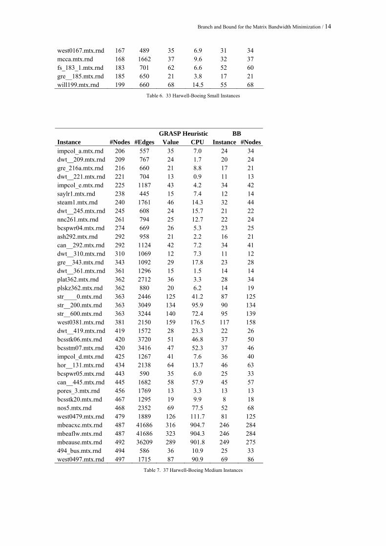
Appendix
GRASP Heuristic BB Instance #Nodes #Edges Value CPU Lbound Uboundpores_1.mtx.rnd 30 103 7 0.2 7 7 ibm32.mtx.rnd 32 90 11 0.2 11 11 bcspwr01.mtx.rnd 39 46 5 0.1 5 5 bcsstk01.mtx.rnd 48 176 16 0.7 16 16 bcspwr02.mtx.rnd 49 59 7 0.3 7 7 curtis54.mtx.rnd 54 124 10 0.5 10 10 will57.mtx.rnd 57 127 7 0.3 6 6 impcol_b.mtx.rnd 59 281 21 0.9 19 21 steam3.mtx.rnd 80 424 7 0.0 7 7 ash85.mtx.rnd 85 219 9 0.3 9 9 nos4.mtx.rnd 100 247 10 1.1 10 10 gent113.mtx.rnd 104 549 27 1.1 25 27 bcsstk22.mtx.rnd 110 254 10 1.0 9 10 gre__115.mtx.rnd 115 267 24 1.9 20 24 dwt__234.mtx.rnd 117 162 12 0.4 11 11 bcspwr03.mtx.rnd 118 179 11 0.4 9 10 lns__131.mtx.rnd 123 275 21 2.0 18 20 arc130.mtx.rnd 130 715 63 1.4 63 63 bcsstk04.mtx.rnd 132 1758 37 2.0 36 37 west0132.mtx.rnd 132 404 36 3.3 23 35 impcol_c.mtx.rnd 137 352 31 3.6 23 30 can__144.mtx.rnd 144 576 14 1.9 13 13 lund_a.mtx.rnd 147 1151 23 3.0 19 23 lund_b.mtx.rnd 147 1147 23 3.0 19 23 bcsstk05.mtx.rnd 153 1135 20 3.5 19 20 west0156.mtx.rnd 156 371 37 5.1 33 37 nos1.mtx.rnd 158 312 3 0.0 3 3 can__161.mtx.rnd 161 608 18 0.8 18 18
Branch and Bound for the Matrix Bandwidth Minimization / 14
west0167.mtx.rnd 167 489 35 6.9 31 34 mcca.mtx.rnd 168 1662 37 9.6 32 37 fs_183_1.mtx.rnd 183 701 62 6.6 52 60 gre__185.mtx.rnd 185 650 21 3.8 17 21 will199.mtx.rnd 199 660 68 14.5 55 68
Table 6. 33 Harwell-Boeing Small Instances
GRASP Heuristic BB Instance #Nodes #Edges Value CPU Instance #Nodesimpcol_a.mtx.rnd 206 557 35 7.0 24 34 dwt__209.mtx.rnd 209 767 24 1.7 20 24 gre_216a.mtx.rnd 216 660 21 8.8 17 21 dwt__221.mtx.rnd 221 704 13 0.9 11 13 impcol_e.mtx.rnd 225 1187 43 4.2 34 42 saylr1.mtx.rnd 238 445 15 7.4 12 14 steam1.mtx.rnd 240 1761 46 14.3 32 44 dwt__245.mtx.rnd 245 608 24 15.7 21 22 nnc261.mtx.rnd 261 794 25 12.7 22 24 bcspwr04.mtx.rnd 274 669 26 5.3 23 25 ash292.mtx.rnd 292 958 21 2.2 16 21 can__292.mtx.rnd 292 1124 42 7.2 34 41 dwt__310.mtx.rnd 310 1069 12 7.3 11 12 gre__343.mtx.rnd 343 1092 29 17.8 23 28 dwt__361.mtx.rnd 361 1296 15 1.5 14 14 plat362.mtx.rnd 362 2712 36 3.3 28 34 plskz362.mtx.rnd 362 880 20 6.2 14 19 str____0.mtx.rnd 363 2446 125 41.2 87 125 str__200.mtx.rnd 363 3049 134 95.9 90 134 str__600.mtx.rnd 363 3244 140 72.4 95 139 west0381.mtx.rnd 381 2150 159 176.5 117 158 dwt__419.mtx.rnd 419 1572 28 23.3 22 26 bcsstk06.mtx.rnd 420 3720 51 46.8 37 50 bcsstm07.mtx.rnd 420 3416 47 52.3 37 46 impcol_d.mtx.rnd 425 1267 41 7.6 36 40 hor__131.mtx.rnd 434 2138 64 13.7 46 63 bcspwr05.mtx.rnd 443 590 35 6.0 25 33 can__445.mtx.rnd 445 1682 58 57.9 45 57 pores_3.mtx.rnd 456 1769 13 3.3 13 13 bcsstk20.mtx.rnd 467 1295 19 9.9 8 18 nos5.mtx.rnd 468 2352 69 77.5 52 68 west0479.mtx.rnd 479 1889 126 111.7 81 125 mbeacxc.mtx.rnd 487 41686 316 904.7 246 284 mbeaflw.mtx.rnd 487 41686 323 904.3 246 284 mbeause.mtx.rnd 492 36209 289 901.8 249 275 494_bus.mtx.rnd 494 586 36 10.9 25 33 west0497.mtx.rnd 497 1715 87 90.9 69 86
Table 7. 37 Harwell-Boeing Medium Instances
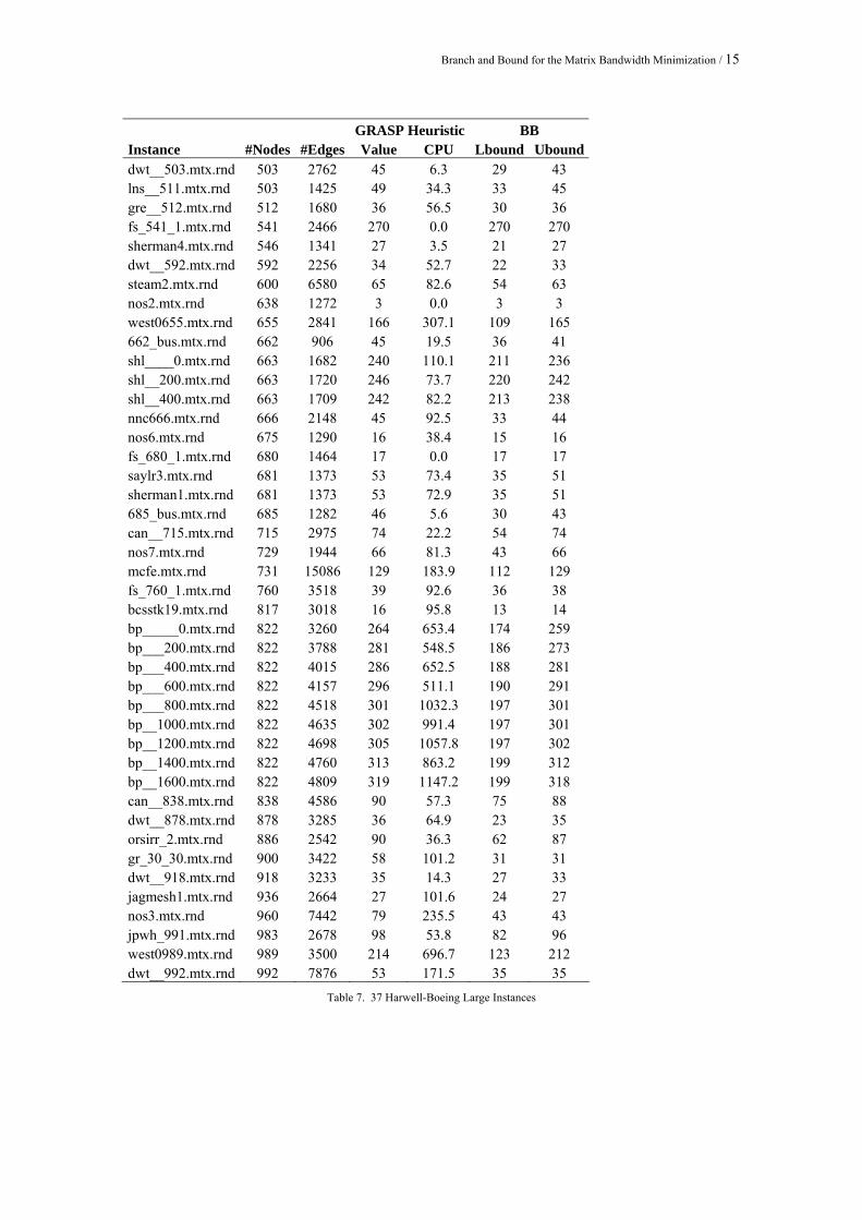
Branch and Bound for the Matrix Bandwidth Minimization / 15
GRASP Heuristic BB Instance #Nodes #Edges Value CPU Lbound Ubounddwt__503.mtx.rnd 503 2762 45 6.3 29 43 lns__511.mtx.rnd 503 1425 49 34.3 33 45 gre__512.mtx.rnd 512 1680 36 56.5 30 36 fs_541_1.mtx.rnd 541 2466 270 0.0 270 270 sherman4.mtx.rnd 546 1341 27 3.5 21 27 dwt__592.mtx.rnd 592 2256 34 52.7 22 33 steam2.mtx.rnd 600 6580 65 82.6 54 63 nos2.mtx.rnd 638 1272 3 0.0 3 3 west0655.mtx.rnd 655 2841 166 307.1 109 165 662_bus.mtx.rnd 662 906 45 19.5 36 41 shl____0.mtx.rnd 663 1682 240 110.1 211 236 shl__200.mtx.rnd 663 1720 246 73.7 220 242 shl__400.mtx.rnd 663 1709 242 82.2 213 238 nnc666.mtx.rnd 666 2148 45 92.5 33 44 nos6.mtx.rnd 675 1290 16 38.4 15 16 fs_680_1.mtx.rnd 680 1464 17 0.0 17 17 saylr3.mtx.rnd 681 1373 53 73.4 35 51 sherman1.mtx.rnd 681 1373 53 72.9 35 51 685_bus.mtx.rnd 685 1282 46 5.6 30 43 can__715.mtx.rnd 715 2975 74 22.2 54 74 nos7.mtx.rnd 729 1944 66 81.3 43 66 mcfe.mtx.rnd 731 15086 129 183.9 112 129 fs_760_1.mtx.rnd 760 3518 39 92.6 36 38 bcsstk19.mtx.rnd 817 3018 16 95.8 13 14 bp_____0.mtx.rnd 822 3260 264 653.4 174 259 bp___200.mtx.rnd 822 3788 281 548.5 186 273 bp___400.mtx.rnd 822 4015 286 652.5 188 281 bp___600.mtx.rnd 822 4157 296 511.1 190 291 bp___800.mtx.rnd 822 4518 301 1032.3 197 301 bp__1000.mtx.rnd 822 4635 302 991.4 197 301 bp__1200.mtx.rnd 822 4698 305 1057.8 197 302 bp__1400.mtx.rnd 822 4760 313 863.2 199 312 bp__1600.mtx.rnd 822 4809 319 1147.2 199 318 can__838.mtx.rnd 838 4586 90 57.3 75 88 dwt__878.mtx.rnd 878 3285 36 64.9 23 35 orsirr_2.mtx.rnd 886 2542 90 36.3 62 87 gr_30_30.mtx.rnd 900 3422 58 101.2 31 31 dwt__918.mtx.rnd 918 3233 35 14.3 27 33 jagmesh1.mtx.rnd 936 2664 27 101.6 24 27 nos3.mtx.rnd 960 7442 79 235.5 43 43 jpwh_991.mtx.rnd 983 2678 98 53.8 82 96 west0989.mtx.rnd 989 3500 214 696.7 123 212 dwt__992.mtx.rnd 992 7876 53 171.5 35 35
Table 7. 37 Harwell-Boeing Large Instances