A Bootstrap-based Non-parametric ANOVA Method with Applications

to Factorial Microarray Data

Baiyu Zhou (zhouby98@stanford.edu)

Department of Statistics, Stanford University, Stanford, CA 94305

Wing Hung Wong* (whwong@stanford.edu)

Department of Statistics, Stanford University, Stanford, CA 94305

Abstract: Many microarray experiments have factorial designs. But there are few

statistical methods developed explicitly to handle the factorial analysis in these

experiments. We propose a bootstrap-based non-parametric ANOVA (NANOVA)

method and a gene classification algorithm to classify genes into different groups

according to the factor effects. The proposed method encompasses one-way and two-way

models, as well as balanced and unbalanced experimental designs. False discovery rate

(FDR) estimation is embedded into the procedure, and the method is robust to outliers.

The gene classification algorithm is based on a series of NANOVA tests. The false

discovery rate of each test is carefully controlled. Gene expression pattern in each group

is modeled by a different ANOVA structure. We demonstrate the performance of

NANOVA using simulated and real microarray data.

Key words and phrases: Bootstrap re-sampling, factorial design, false discovery rate

estimation, gene classification, microarray, non-parametric ANOVA, robust test.

*To whom correspondence should be addressed

1. Introduction

Microarray technology is a powerful tool to monitor gene expression levels on a

genome scale. An important question in microarray experiments that has been studied

extensively is the identification of differentially expressed genes across two or more

biological conditions. Many statistical methods have been developed to address this

problem, for instance, Baldi & Long (2001), Efron, Tibshirani, Storey & Tusher (2001),

Tusher, Tibshirani & Chu (2001), Dudoit, Yang, Callow & Speed (2002), Newton,

Noueiry, Sarkar & Ahlquist (2004). Typically a summary statistic is constructed for each

gene and genes are ranked in order of their test statistics. Genes with test statistics above

a chosen threshold are called significant. Empirical Bayes method treats genes arising

from different populations (Efron, Tibshirani, Storey & Tusher 2001). A gene is called

significant if its estimated posterior odds of having differential expression is larger than

the threshold. The significant analysis of microarray (SAM) (Tusher, Tibshirani & Chu

2001) employs a permutation approach to simulate null distribution of test statistic and

estimate false discovery rate (FDR). A threshold is then chosen based on the estimated

FDR.

However a microarray experiment often has a factorial design and involves several

experimental factors. For example, in one experiment, a growth factor (FGF) was

withdrawn from two proliferating stem cell lines (neuron and glia) to accelerate the

differentiation process (Goff, Davila, Jornsten, Keles & Hart 2007). Gene expressions

were measured at different times after FGF withdrawn. Investigators were interested in

how genes in two cell lines responded to FGF withdrawal along time. In this experiment,

cell-line and time course can be treated as two factors. Most current methods were not

designed to handle such factorial experiments. There have been a few studies proposing

using the analysis of variance (ANOVA) or its modified versions in microarray data

analysis (Pavlidis & Noble 2001; Gao & Song 2005). ANOVA is a classical method for

factorial data analysis. It decomposes data variation into variations accounted by different

factors. Contribution of each factor is assessed by F -statistic. Applying ANOVA to the

stem cell experiment allows one to identify gene having cell-line effect or time effect, as

well as ‘interaction genes’. These genes are often of great interest to biologists. In the

above example, interaction genes are those having different response patterns along the

time course in different cell lines. However, direct application of standard ANOVA to

microarray data could be problematic. First, F -test makes normality assumption about

the data distribution, which is often untenable in microarray studies; Second, an

appropriate cutoff based on computed F -statistics or p-values is difficult to choose. In

multiple-testing problems, error rate should be controlled based on FDR rather than p-

values; Third, presence of outliers in microarray data could deteriorate statistical power,

in which case a robust statistical procedure may be required. To relax distributional

assumptions, rank-based non-parametric ANOVA have been proposed (Friedman 1937;

Conover & Iman 1979; Gao & Song 2005). Empirical p-values are computed by

permuting the data. It has been pointed out that the permutation approach may not lead to

the appropriate null distribution (Pan 2003; Gao 2006). When the microarray data contain

a large proportion of non-null genes, permutation distribution is the mixture of

permutation distribution under null hypothesis and permutation distribution under

alternative hypothesis, which is not a good approximation of true null distribution. Jung,

Jhun & Song (2007) proposed an exact permutation test which permutes residuals of data

instead of observed data. Their method is restricted to balanced experimental designs. A

carefully schemed subpartition procedure has also been proposed in non-parametric

ANOVA to simulate null distributions (Gao 2006). But the procedure requires at least

four replicates in each biological condition and assumes symmetric noise distribution.

Motivated by factorial microarray experiments and limitations of existing ANOVA

methods, we develop a non-parametric ANOVA method (NANOVA), which constructs

null distributions by bootstrap re-sampling. FDR estimation is naturally embedded into

the procedure. NANOVA encompasses one-way and two-way models as well as balanced

and unbalanced experimental designs. A robust test is proposed to protect against outliers

when enough replicates are available. For two-way factorial experiments, we propose a

gene classification algorithm which classifies genes into different groups by how their

expressions are influenced by factors. The gene classification algorithm is based on a

series of NANOVA tests with the error rate of each test controlled by FDR.

The proposed method was applied to two microarray studies. In the first study, we

analyzed gene expression data from two human lymphoblastioid cell lines growing in an

unirradiated state or in an irradiated state, and compared our method to the SAM method

(Tusher, Tibshirani & Chu 2001) and a linear model with moderated F-statistics (‘limma’)

(Yang & Speed 2002; Diaz et al. 2002; Smyth 2004). The second microarray data were

from six brain regions in two mouse strains (Sandberg et al. 2000). We analyzed the

effects of strain and brain region on the gene expression and compared with the results

obtained from the standard ANOVA method (Pavlidis & Noble 2001).

2. Method

We first introduce some notations for two-way factorial experiments. Let

( 1,..., )i

i Iα = and ( 1,..., )j

j Jβ = denote the two factors of interest at level i and j

respectively. Let ,g ijky be the expression of gene g under condition ( , )

i jα β . Here

( 1,..., )ij

k k n= is a subscript for replicates. We model the gene expressions as a response

variable and factors as explanatory variables. In two-way factorial experiments, gene

expression can be summarized by one of the following ANOVA models. For simplicity,

subscript g will be dropped.

Model (1): ijk i j ij ijk

y eµ α β γ= + + + + (2.1)

Model (2): ijk i j ijk

y eµ α β= + + + (2.2)

Model (3): ijk i ijk

y eµ α= + + (2.3)

Model (4): ijk j ijk

y eµ β= + + (2.4)

Model (5): ijk ijk

y eµ= + (2.5)

Model (1) is an interactive model. µ represents the baseline gene expression level. ij

γ is

the interaction term. Genes of model (1) are influenced by both factors, and the effect of

one factor is dependent on the level of the other factor. Model (2) is an additive model.

Genes of model (2) are affected by both factors, but factor effects are independent. Genes

of model (3) and (4) have only α or β effect. Genes of model (5) are not influenced by

either factor. We assume the random error ijk

e is independent identically distributed from

a gene specific distribution. Constraints 0i

i

α =∑ , 0j

j

β =∑ and 0ij ij

i j

γ γ= =∑ ∑ are

imposed for identifiability.

We will classify genes into five groups ( 1 2 3 4, , ,C C C C and 5C ). Each group

corresponds to one of the above models. The classification will be based on a series of

NANOVA tests.

2.1 NANOVA test

The proposed NANOVA method includes tests for one-way ANOVA, interaction and

main effects of two-way ANOVA. Details are given in the following section.

(1) One-way NANOVA test

In this test we treat (2.5) as the null hypothesis and test it against the alternatives that

the mean expression of the gene is not constant across all combinations of the two factors.

The null hypothesis ijk ijk

y eµ= + implies gene expression is not influenced by either

factor. We choose as our test statistic the standard one way ANOVA F

statistic 2 2

1 . .

1 1 1 1 1 1

[ ( ...) /( 1)] /[ ( ) /( )]ij ijn nI J I J

ij ijk ij

i j k i j k

F y y IJ y y N IJ= = = = = =

= − − − −∑∑∑ ∑∑∑ ,

where .

1

1 ijn

ij ijk

kij

y yn =

= ∑ , ...

1 1 1

1 ijnI J

ijk

i j k

y yN = = =

= ∑∑∑ andij

i j

N n=∑∑ . The dot. used as a subscript

indicates that the summation is taken over the corresponding subscript and an average is

taken by dividing by the number of terms in the sum. The numerator and denominator of

1F are estimations of between group variance and within group variance. Under the

normality assumption, null distribution of 1F is the F distribution with degrees of

freedom ( 1, )IJ N IJ− − . Instead of replying on the normality assumption, we simulate the

null distribution of 1F by bootstrap re-sampling as follows:

1. Sampling *

ijkε ( 1,2,... ; 1, 2,... ; 1, 2,... )

iji I j J k n= = = with replacement

from .ijk ijk ijy yε = − .

2. Let * *

...ijk ijky y ε= + and compute null statistic *

1F using the null data *

ijky .

3. Repeat step 1 and 2 B times to get (1)* (2)* ( )*

1 1 1, ,... BF F F .

In step 1, bootstrap re-sampling of *

ijkε is used to simulate the random error

distribution. We estimate the random error by not assuming any specific model form but

utilizing the replicated micoarray samples. In step 2, *

ijky is generated from the null model

by adding the re-sampled residuals to the estimated mean under the null model (2.5). Step

3 repeats bootstrap B times to simulate the null distribution of 1F . NANOVA allows an

unspecified random error distribution, and constructs null data by adding the bootstrap re-

sampled residuals to the null model. The same idea will be applied to interaction and

main effect tests.

(2) Interaction effect NANOVA test

The null hypothesis of no interaction effect is 0 :H 0ij

γ = ( 1,... , 1,...i I j J= = ) in

model (1). For balanced experimental designs, interaction effect is estimated by

. .. . .ˆ ...

ij ij i jy y y yγ = − − + . The test statistic is defined as

2

. .. . . ...

2 2

.

( ) /[( 1)( 1)]

( ) /[ ( 1)]

ij i j

i j

ijk ij

i j k

k y y y y I J

Fy y IJ k

− − + − −

=− −

∑∑

∑∑∑, where k is the number of replicates in

each condition. The denominator of 2F is an estimation of the random error variance. The

numerator of 2F estimates the sum of squares of the interaction effect. When

experimental designs are unbalanced, ij

γ cannot be estimated as above. We use the idea

of ‘un-weighted cell mean’ (Searle, Casella & Mcculloch 1992) to estimateij

γ .

Specifically, let .ij ijx y= (cell mean), then

ijγ is estimated by . . ..ij ij i j

x x x xγ = − − − ,

where . .

1 1

/ , /J I

i ij j ij

j i

x x J x x I= =

= =∑ ∑ and ..

,

/ij

i j

x x IJ=∑ . Test statistic for unbalanced

experimental design is defined

as 2 2

2 . . .. .

1 1 1 1 1

( ) /[ ( ) /( )]ijnI J I J

ij i j ijk ij

i j i j k

F x x x x y y N IJ= = = = =

= − − + − −∑∑ ∑∑∑ . The null distribution of

the test statistic is simulated as follows:

1. Sampling *

ijkε ( 1,... ; 1,... ; 1,... )

iji I j J k n= = = with replacement from .ijk ijk ij

y yε = − .

2. Let* *ˆˆˆijk i j ijk

y µ α β ε= + + + , where ˆˆˆ( , , )i j

µ α β are the least square estimates from the

null modelijk i j ijk

y eµ α β= + + + . Compute null statistic *

2F by using the null

data *

ijky .

3. Repeat step 1 and 2 B times to get (1)* (2)* ( )*

2 2 2, ,... BF F F .

(3) Main effect NANOVA test

The main effect i

α is estimated by .. ...ˆ

i iy yα = − if the experimental design is balanced.

For unbalanced design, we use ‘un-weighted cell mean’ to estimatei

α . The estimate is

.. ...ˆ

i ix xα = − , where ..i

x and ...x are defined as above. The test statistic is defined as

2 2

3 .. ... .( ) /( 1) /[ ( ) / ( 1)]i ijk ij

i j i j k

F k y y I y y IJ k= − − − −∑∑ ∑∑∑ or

2 2

3 . .. .

1 1 1

( ) /[ ( ) /( )]ijnI J

i ijk ij

i i j k

F x x y y N IJ= = =

= − − −∑ ∑∑∑ for balanced or unbalanced design

respectively. The null distribution of 3F is simulated as follows:

1. Sampling *

ijkε ( 1,... ; 1,... ; 1,... )

iji I j J k n= = = with replacement from .ijk ijk ij

y yε = −

2. Let* *ˆˆijk j ijk

y µ β ε= + + , where ˆˆ( , )j

µ β are the least square estimates from the null

modelijk j ijk

y eµ β= + + . Compute *

3F by using the null data *

ijky .

3. Repeat step 1 and 2 B times to get (1)* (2)* ( )*

3 3 3, ,... BF F F .

2.2 Robust NANOVA test

Standard ANOVA test is susceptible to poor performance in the presence of outliers.

Since outliers are unavoidable in large microarray data sets, we guard against them by

using robust estimators for mean and variance estimations in test statistics. For example,

in the one-way ANOVA test

2 2

1 . .

1 1 1 1 1 1

( ...) /( 1) /[ ( ) /( )]ij ijn nI J I J

ij ijk ij

i j k i j k

F y y IJ y y N IJ= = = = = =

= − − − −∑∑∑ ∑∑∑ , the mean estimator .ijy

and ...y are replaced by trimmed means. The between variance estimator

2

.

1 1 1

( ...)ijnI J

ij

i j k

y y= = =

−∑∑∑ is replaced by the trimmed mean taken over

2

.( ...) ( 1,.., ; 1,.., ; 1,.., )ij ij

y y i I j J k n− = = = times the number of items (,

ij

i j

n∑ ). Similar

robust estimator is used for the within variance estimation in the denominator of 1F . Null

distribution of the robust statistic does not have an analytical form, but its empirical

distribution is easily obtained by the bootstrap re-sampling.

2.3 FDR estimation

In multiple testing problems, it is important to control the false discovery rate (FDR)

which is defined as the expected proportion of false rejections among all rejections

(Benjamini et al. 1995). The proposed NANOVA procedure provides a natural way for

estimating FDR. Let ( 1,..., )g

F g G= be the statistic computed from the observed data, g

is the gene index. Significance of g

F is assessed against the null distribution generated by

the bootstrap re-sampling. At each bootstrap, we sample the array labels. The

corresponding vector of residuals , , .{( ), 1,..., }g ijk g ij

y y g G− = from the same array is kept

intact. Such bootstrap operation preserves correlations between genes. Empirical p-value

for gene g is computed by ( )*#{ : 1,..., }/j

g g gp F F j B B= ≥ = , where B is the number of

bootstraps. FDR can be estimated from empirical p-values. However when the number of

bootstraps or permutations is limited by the sample size or computation cost, the resulting

p-values may be too granular to allow a sensible FDR estimation. We propose the

following alternative approach to estimate FDR:

1. Estimate a null distribution for each gene. In NANOVA, we fit a Gamma

distribution to the null statistics (1)* ( )*,..., B

g gF F for each gene g . The reason to use

Gamma distribution is because it is flexible enough to capture most of

distributions with positive support. The parameters of Gamma distribution can be

robustly estimated by using a few quantile points (for example, 10%, 25%, 50%,

75% and 90% quantiles of (1)* ( )*,..., B

g gF F ). An alternative approach is to use an

iterative fitting procedure, i.e. fit a Gamma distribution, trim off extreme data

points (if any) and refit the rest data. The process is repeated a few times. Denote

the cumulative function of Gamma distribution asg

G .

2. Transform test statistics and null statistics to z-scores by the transformation

1( ( ))g g g

z G F−= Φ , where ( )Φ ⋅ is the cumulative function of the standard normal

distribution.

3. Given a cut off *d , genes with *( 1,..., )g

z d g G> = are called significant. FDR is

estimated as 0

1

ˆ ( ) /( )B

j

V j RBπ=

∑ , where *#{ : , 1,..., }g

R g z d g G= > = is the number

of significant genes, and ( )* *( ) #{ : , 1,..., }j

gV j g z d g G= > = is an estimate of the

number of false rejections using j th bootstrapped data if all genes are null. 0π is

an estimation of the proportion of null genes. At j th bootstrap, let

* ( )*{ }maxj

j gg

z z= be the maximum ( )*j

gz over G genes. An overestimation for the

number of null genes is *( ) #{ : }g j

M j g z z= ≤ . 0π is taken as the median of

( ) / ( 1,..., )M j G j B= .

The FDR estimation procedure does not assume the same null distribution for all

genes, but instead transforms the significance measures of genes to the same scale and

makes them comparable across genes. Genes are ranked by g

z .

2.4 Gene Classification algorithm

Depending on how their expressions are influenced by factors, genes can be classified

into different groups ( 1 2 3 4, , ,C C C C and 5C ). Each corresponds to an ANOVA model. 1C

is an interaction group, whose genes are affected by both factors, and factor effects are

dependant (model (1)). 2C is an additive group. Genes in 2C are affected by factors, but

factor effects are independent (model (2)). Genes from 3C or 4C have only α (model (3))

or β effect (model (4)). Genes in 5C are not affected by either factor (model (5)). The

classification is based on a series of NANOVA tests. Error rate of each test is controlled

by FDR. The algorithm is as follows:

1 First identify genes whose expressions are affected by factor α or β . This is

done by treating each condition ( , )i j

α β as a group, and performing one-way

NANOVA. Denote this group of genes as S .

2 Within S , identify interaction genes by interaction NANOVA test. The

resulted gene set is 1C .

3 Among the remaining genes ( 1S C− ), use main effect NANOVA tests to identify

genes having α and β effect respectively. Denote these two sets as Sα and Sβ .

Then 3 ( )C S S Sα β α= − ∩ and 4 ( )C S S Sβ β α= − ∩ .

4 Genes in 1 3 4S C C C− − − are classified to 2C .

5 The rest of genes are classified to 5C

3. Simulation Studies

3.1 Bootstrapped null distribution

The key part of NANOVA tests is the simulation of null distribution. To test how well

the bootstrapped null distributions approximate true nulls, we simulated expressions of

1000 genes in a two-way factorial experiment. Genes 1-100 were generated from model

(1), 101-200 from model (2), 201-300 from model (3), and 301-400 from model (4). The

rest genes were from model (5). Each factor has two levels. There are 7 replicates under

each condition ( , )i j

α β . Parameters ( , , , )i j ij

µ α β γ were independently drawn from

uniform[ 5,5]− , and subjected to the constraints 0i

i

α =∑ , 0j

j

β =∑ , 0ij ij

i j

γ γ= =∑ ∑ .

The random error was generated from standard normal (0,1)N . We first constructed null

statistics for one-way NANOVA test. The number of bootstraps is set to be 100B = .

Kolmogorov-Smirnov (KS) test was used to test the deviation of the bootstrapped null

distribution of each gene from the true null (3, 24)F . The numbers in parenthesis are

degrees of freedom of the F distribution. If the bootstrapped nulls were consistent with

the true null, the p-values resulted from KS tests should follow the uniform distribution.

We can apply again KS test to verify if these p-values are uniformly distributed. This

nested-KS test has been used by Leek & Storey (2007). After applying the nested-KS test,

we obtained a p-value of 0.25, indicating the bootstrapped null distributions were

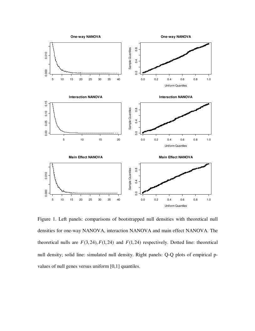
consistent with the true null. The tail of null distribution is important for assessing

statistical significance. The left panel of Figure 1 compares the tail density of the

bootstrapped nulls and the true null.

Next we tested if the empirical p-values obtained from one-way NANOVA were

correct. The correct p-values corresponding to null genes should be uniformly distributed

between zero and one. KS test on the empirical p-values of the null genes (genes 401-

1000) (compared with the uniform distribution) yielded a p-value of 0.29, indicating the

empirical p-values of the null genes were uniformly distributed. Right panel of Figure 1

shows a Q-Q plot of these empirical p-values versus the uniform distribution.

Similar comparisons were done on the interaction and main effect NANOVA tests. P-

values of 0.22 and 0.87 were obtained from the nested-KS tests for the interaction and

main effect tests respectively. Empirical p-values of the null genes (genes 101-1000 for

interaction effect; genes 301-1000 for main effectα ) were uniformly distributed in [0,1]

(Figure 1) with the p-values of 0.35 and 0.22 by the KS test.

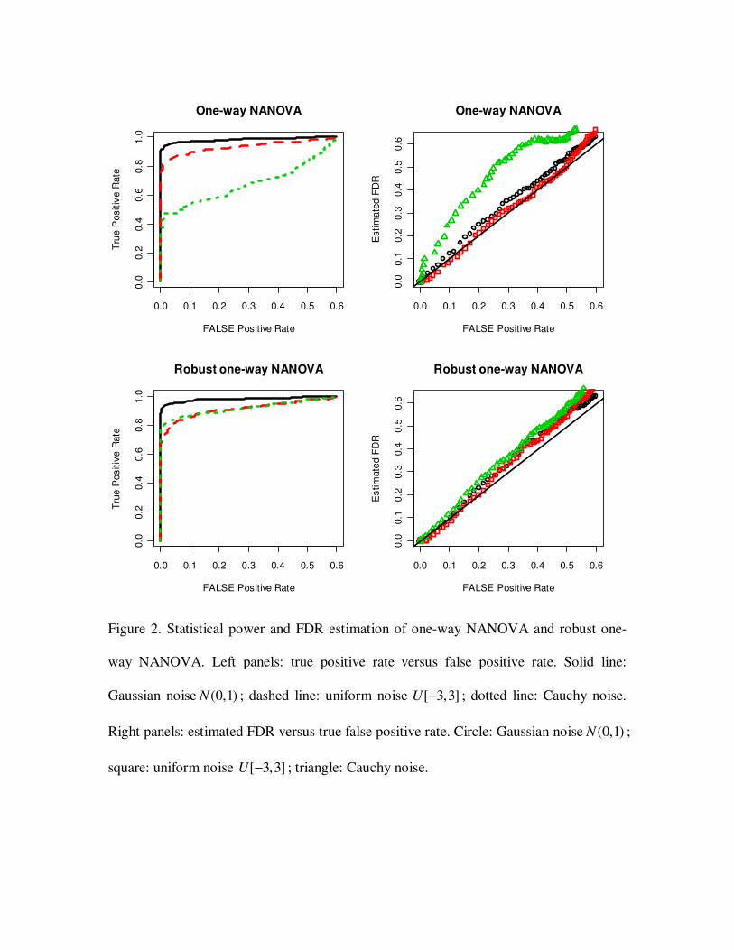
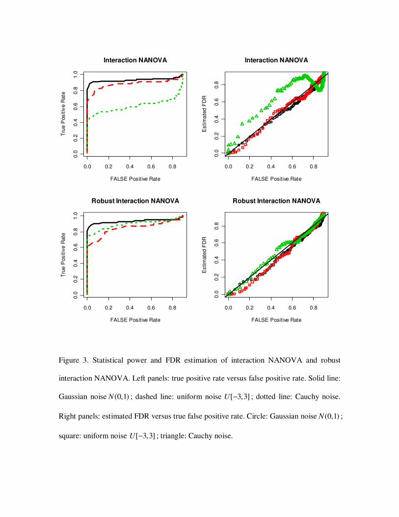
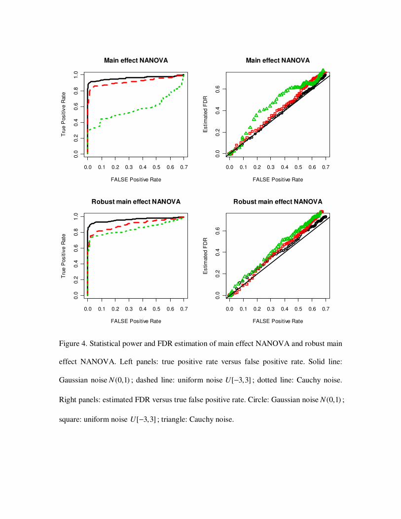
3.2 Statistical power and FDR estimation

To test the ability of NANOVA to identify true positive genes, we simulated three data

sets. Each data set consists of 1000 genes, and was generated as in section 3.1. The three

data sets had different error distributions: (1) normal (0,1)N ; (2) uniform [ 3,3]− ; (3)

Cauchy distribution. Genes were ranked by g

z (section 2.4). Given a cut off *d , genes

with *

gz d> were called significant. Proportions of identified true positives (power)

versus proportions of false positives (ROC curves) are shown in Figure 2, 3 and 4. All

three tests showed good statistical power for selecting true positive genes when the

random error was normally or uniformly distributed. However, in the Cauchy case, a

large fraction of outlier deteriorated statistical power.

We also compared estimated FDR and true false positive rates with varied cut offs

(Figure 2, 3 and 4). The estimated FDR was in a good agreement with the true false

positive rate in normal and uniform cases. In Cauchy case, the outliers made the FDR

estimation inaccurate.

3.3 Robust NANOVA test

Outliers commonly exist in microarray data. They could potentially deteriorate

statistical power and make FDR estimation inaccurate as in the above simulations. When

there are enough replicates, NANOVA procedure can be robustified by using robust

estimators for the mean and variance estimations in the test statistic. We applied robust

NANOVA tests on the same data sets in 3.2 and compared statistical power and FDR

estimation. Trimmed mean which discards 20 percent data of both ends was used. As

shown in Figure 2, 3 and 4, robust NANOVA tests greatly improved statistical power

when the data were noisy (Cauchy case). FDR was also more accurately estimated by

robust NANOVA.

4. Applications to Biological Data

4.1 Ionizing radiation data

To demonstrate the utility of NANOVA method, we analyzed the microarray data

measuring transcriptional response of lymphoblastoid cells to ionizing radiation (IR)

(Tusher, Tibshirani & Chu 2001, data were downloaded from http://www-

stat.stanford.edu/~tibs/SAM/). The experiments were performed for two wild-type human

lymphoblastioid cell lines (1 and 2) growing in an unirradiated state (U) or in an

irradiated state (I). There are two replicates in each condition (A and B). The data set

consists of expressions of 7129 genes in eight samples (U1A, U1B, I1A, I1B, U2A, U2B,

I2A and I2B). To assess the biological effect of IR, SAM used a restricted permutation

approach which balanced the two cell lines to avoid confounding effects from differences

between the cell lines. To achieve the same goal, we treated the cell lines and IR states as

two factors and applied NANOVA main effect test to identify genes responding to IR.

Another approach is to fit a linear model g g

Y Xθ ε= + for each gene g . g

Y is a vector of

expressions from the eight samples, X is the design matrix, g

θ is a vector of parameters

of interest, and ε is the error. The elements of ( )1 2, , , 'g

m c r rθ = represent intercept,

cell line effect, IR effect in cell line 1 and IR effect in cell line2 respectively. Genes

responding to IR in either cell line can be identified by computing a moderated F-statistic

derived from the linear model (Yang & Speed 2002; Diaz et al. 2002; Smyth 2004). We

used ‘limma’ software for the computation (Smyth 2004). Limma controls FDR by

adjusting p-values using the Benjamini and Hochberg (BH) method. The significance

results are displayed in Table 1. It can be seen NANOVA method offers a sizeable

increase in statistical power over SAM or limma. The restricted permutation in SAM

analysis failed to identify genes responding to IR in one cell line but not the other (Figure

5) and has limited power in analyzing factorial data. The linear model is able to handle

factorial designs, but the moderated F-statistic derived from normal theory may result

incorrect p-value when microarray data are not normally distributed. Limma does not

offer a sensible FDR control mechanism. Its use of conservative ‘BH’ approach may lose

statistical power in discovering significant genes.

To confirm the improvement of statistical power of NANOVA over SAM or limma,

we simulated expression profiles of 1000 genes based on the IR data. We fitted a two-

way ANOVA model for every gene in the IR data and chose 200 genes with significant

IR effect (p-value<0.05) but no cell line effect (p-value>0.2) as well as 800 genes without

significant IR effect (p-value>0.8). Let ijk

y denote expression of a gene in the IR data.

,i j and k indicate cell line, IR state and replicates respectively. Let .ijk ijk ijy yε = − We

simulated random error of gene expression by *

ijkε , where *

ijkε is a permutation of

ijkε . For

the first 200 genes, we estimated the IR effect by . . ...jy y− and simulated their expression

by * *

... . . ...( )ijk j ijk

y y y y ε= + − + . For the rest 800 genes, the simulated expressions were set

to * *

... .. ...( )ijk i ijk

y y y y ε= + − + . Therefore, we generated a data set with the error distribution

close to the real microarray data. The first 200 genes were known to be IR responsive and

we compared the performance of NANOVA, SAM and limma to identify them. We also

computed the false positive rate (FPR) and true positive rate (TPR), defined as:

{#false rejected genes}

{#rejected genes}FPR = and

{#correctly rejected genes}

{# true positive genes}TPR = . Table 2 shows the

significant results under different FDR cutoffs. Although the simulation setting was in

favor of SAM, NANOVA still outperformed SAM in terms of statistical power. Limma

had the least power on this data set. Instead of BH adjustment limma uses, a less

conservative approach for FDR control is to use the q-value method (Storey & Tibshirani

2003). A FDR cutoff was chosen based on the computed q-values. As can bee seen from

Table 2, the q-value method offered a slight improvement over BH adjustment but still

excluded many true positive genes. This suggests the p-values computed by limma may

not be correct as the data distribution were not normal.

4.2 Mouse brain data

We applied the proposed method to analyze gene expression data of six brain regions

(amygdala, cerebellum, cortex, entorhinal cortex, hippocampus and midbrain) in two

mouse strains (C57BL/6 and 129SvEv) (Sandberg et al. 2000). Data were obtained from

Pavlidis & Noble (2001). Gene expression profiles were measured by using

oligonucleotide arrays (Mu11KsubA and Mu11KsubB). The dataset consists of duplicate

measurements of 13067 probe sets, providing a rich source to study the genetic causes

responsible for neurophysiological differences in two mouse strains. Factors of interest

are strains and brain regions. It is interesting to identify strain specific and region specific

genes

We applied the gene classification algorithm to the dataset (log2 transformed). FDR

was controlled at 0.05 for the NANOVA tests. Probe sets were classified into five groups

according to the factor effects. As a result, 1 2 3, ,C C C and 4C have 126, 167, 31 and 742

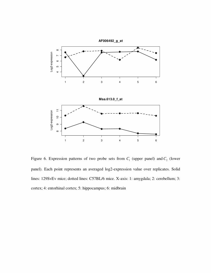
probe sets respectively. Figure 6 shows the expression pattern of two representative probe

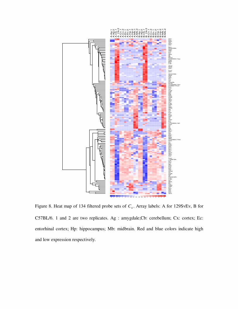
sets from gene set 1C and 2C . Figure 7 and 8 are heat maps of 3C and 134 probe sets of

4C (filtered by CV (coefficient of variation) > 0.2) generated by dChip (Li & Wong

2001).

1C probe sets had interaction effect and potentially contribute to neurobehavioral

difference of mouse strains. One example is gene Cks2, which was highly expressed in

midbrain of C57BL/6 mice but not in other brain regions or in 129SvEv mice. Protein

encoded by Cks2 binds to the catalytic subunit of the cyclin dependent kinases and is

essential for their biological function. Probe sets in 2C were influenced by both factors,

but factor effects were independent. Expressions over six brain regions were parallel for

two mouse strains, but their values had a vertical shift. Gas5 gene from 2C is known to

harbor mutations in 129SvEv strains that alter mRNA stability (Sandberg et al. 2001).

This stability difference is likely to account for the 2 fold decrease in mRNA abundance

in 129SvEv compared with C57BL/6. Since it was in 2C , all six brain regions were

uniformly affected by the mutation. 2C genes could cause neurobehavioral difference in

strains by influencing the gene expression levels. Expressions of 3C probe sets varied

between strains but not over brain regions. As shown in Figure 7, these 31 gene

expressions were uniformly highly or lowly expressed in one strain, and had an opposite

pattern in the other strain. Hnrpc and Txnl4 are genes involved in mRNA metabolic

process. 4C genes were brain region specific, but equivalently expressed in both strains.

The heat map reveals cerebellum is the most distinct region among the six brain regions.

A large proportion of genes were up or down regulated in cerebellum but not in other

regions. Pcp2, a known cerebellar specific gene (Sandberg et al. 2001) had about 3 fold

increased expression in cerebellum compared with other regions. We did functional

enrichment analysis on gene set 4C using the web tool built by Dennis et al. (2003)

(http://david.abcc.ncifcrf.gov/). The most significant functional groups (Category:

GOTERM_BP_5) include: neurite morphogenesis (27 genes, p-value: 1.7E-9), neuron

development (31 genes, p-value: 2.8E-9), neuron differentiation (35 genes, p-value: 4.6E-

9), cellular morphogenesis during differentiation (27 genes, p-value: 2.2E-8) and

neurogenesis (38 genes, p-value: 2.4E-8).

In the analysis of Sandberg et al. (2001), they identified 24 probe sets showing

expression variation between strains and about 240 probe sets differentially expressed

over brain regions. They used an ad hoc approach of ‘fold change’ and ‘absent/present’

calls for gene selection, which was rather insensitive to detect significant genes. In a

more elaborate analysis, Pavlidis and Noble (2001) applied standard two-way ANOVA to

the same data set. They tested interaction effect as well as main effects (strains and brain

regions). Under the cutoff of p-value< 510− , they identified 65 strain specific probe sets,

approximately 600 region specific probe sets and 1 probe set with interaction effect. The

choice of p-value< 510− is arbitrary and may be too conservative to include many

interesting genes. Our analysis yielded 324 strain dependant probe sets (probe sets

from 1C , 2C and 3C ) which includeded all 24 probe sets identified by Sandberg et al. and

65 probe sets identified by Pavlidis and Noble (2001).

5. Discussion

In this paper we proposed a bootstrap-based non-parametric ANOVA (NANOVA)

method and a gene classification algorithm for the analysis of factorial microarray data.

We have used simulated and real data sets to demonstrate the utility of our method. There

have been a number of non-parametric methods for microarray data analysis in literature.

Most of them are restricted to two-sample or multi-sample comparisons. When the

experiment involves multiple factors, these methods are less powerful than NANOVA. In

the IR example, in order to identify IR responsive genes, SAM uses restricted

permutation which sacrifices statistical power comparing with explicitly dealing with the

multiple factors. More importantly, NANOVA allows identifying genes with interaction

effects, which are often of great interest to biologists. A major innovation of NANOVA is

in the estimation of null distributions based on bootstrap. The random error is estimated

by utilizing replicated microarray samples and is free of model assumptions. The

permutation approach estimates the null distribution by treating all samples equally and

does not use the information provided by the replicated samples. As a consequence, the

bootstrap approach better estimates the null distribution in the presence of a large

proportion of non-null genes compared to the permutation approach. NANOVA offers a

sensible FDR control which enables the method more powerful in multiple testing over

other methods such as standard ANOVA or limma. The gene classification nicely

summarizes effects of multiple factors in a rather complicated experimental design as

demonstrated in the analysis of mouse data.

Acknowledgement

This research was partially supported by National Institutes of Health grants [R01-

HG004634, R01-HG003903].

References

Baldi P, Long AD (2001). A Bayesian framework for the analysis of microarray

expression data: regularized t-test and statistical inferences of gene changes.

Bioinformatics 17, 509–519.

Benjamini Y, Hochberg Y (1995) Controlling the false discovery rate: a practical and

powerful approach to multiple testing. J. R. Statiat. Soc. Ser. B 57, 289–300.

Conover WJ, Iman RL (1976) On some alternative procedures using ranks for the

analysis of experimental designs. Communications in Statistics A5:1349-1368.

Dennis G. Jr, Sherman BT, Hosack DA, Yang J, Gao W, Lane HC, Lempicki RA (2003)

DAVID: Database for Annotation, Visualization, and Integrated Discovery. Genome

Biology 4(5):P3.

Diaz, E., Ge, Y., Yang, Y.H., Loh, K.C., Serafini, T.A., Okazaki, Y., Hayashizaki, Y.,

Speed, T.P., Ngai, J. and Scheiffele, P. (2002) Molecular analysis of gene expression in

the developing pontocerebellar projection system, Neuron, 36, 417-434.

Dudoit S, Yang YH, Callow MJ, Speed TP (2002) Statistical methods for identifying

differentially expressed genes in replicated cDNA microarray experiments. Statistica

Sinica 12, 111–139

Efron B, Tibshirani R, Storey JD, Tusher V (2001) Empirical Bayes analysis of a

microarray experiment. J. Am. Stat. Assoc. 96, 1151–1160.

Friedman M (1937) The use of ranks to avoid the assumption of normality implicit in the

analysis of variance. Journal of the American Statistical Association 32 (200): 675–701.

Gao X, Song PX (2005) Nonparametric tests for differential gene expression and

interaction effects in multi-factorial microarray experiments. BMC Bioinformatics. Jul 21;

6:186.

Gao X (2006) Construction of null statistics in permutation-based multiple testing for

multi-factorial microarray experiments. Bioinformatics 22(12):1486-1494

Goff LA, Davila J, Jörnsten R, Keles S, Hart RP (2007) Bioinformatic analysis of neural

stem cell differentiation. Journal of Biomolecular Techniques 18:205–212.

Jung B, Jhun M, Song S (2007) A new random permutation test in ANOVA models

Statistical Papers. Vol 48 pp 47-62.

Leek JT, Storey JD (2007) Capturing heterogeneity in gene expression studies by

surrogate variable analysis. PLoS Genet. 1724-35.

Li C, Wong WH (2001) Model-based analysis of oligonucleotide arrays: expression

index computation and outlier detection. Proc Natl Acad Sci. 98(1):31-6.

Newton MA, Noueiry A, Sarkar D, Ahlquist P (2004) Detecting differential gene

expression with a semiparametric hierarchical mixture method. Biostatistics 5(2):155-76

Pan W (2003) On the use of permutation in and the performance of a class of

nonparametric methods to detect differential gene expression. Bioinformatics 19, 1333–

1340.

Pavlidis P, Noble WS (2001) Analysis of strain and regional variation in gene expression

in mouse brain. Genome Biol. 2(10).

Sandberg R, Yasuda R, Pankratz DG, Carter TA, Del Rio JA, Wodicka L, Mayford M,

Lockhart DJ, Barlow C (2000) Regional and strain-specific gene expression mapping in

the adult mouse brain. Proc Natl Acad Sci 97:11038-11043.

Searle S, Casella G, Mcculloch C (1992). Variance Components. New York: Wiley.

Smyth, GK (2004). Linear models and empirical Bayes methods for assessing differential

expression in microarray experiments. Statistical Applications in Genetics and Molecular

Biology 3, No. 1, Article 3.

Storey JD, Tibshirani R. (2003) Statistical significance for genomewide studies. Proc.

Natl Acad. Sci. 100:9440–9445.

Tusher VG, Tibshirani R, Chu G (2001) Significance analysis of microarrays applied to

the ionizing radiation response. Proc. Natl Acad. Sci. 98, 5116–5121.

Yang, Y.H., and Speed, T.P. (2002). Design issues for cDNA microarray experiments.

Nat. Rev. Genet. 3, 579–588.

FDR cutoff NANOVA SAM limma

0.05 206 36 29

0.1 236 69 55

0.2 311 118 136

Table 1. A comparison of the number of genes called significant as found by a NANOVA

test, a SAM test and a moderated F test from linear model (limma). Shown is a

comparison of the proposed method (NANOVA) to a SAM test and a limma test. IR

responsive genes were identified under different FDR cutoffs.

FDR cutoff NANOVA

(FPR/TPR)

SAM

(FPR/TPR)

Limma (BH)

(FPR/TPR)

Limma (qvalue)

(FPR/TPR)

0.01 131 (0/0.655) 97 (0/0.485) 12 (0/0.06) 14 (0/0.07)

0.05 161 (0/0.805) 135(0.02/0.665) 49 (0/0.245) 57 (0/0.285)

0.1 186 (0.03/0.91) 157(0.04/0.755) 74 (0/0.31) 85 (0/0.425)

0.2 216 (0.09/0.99) 188 (0.10/0.85) 128 (0/0.64) 143 (0.02/0.7)

Table 2. A comparison of the number of genes called significant as found by a NANOVA

test, a SAM test and a limma test with BH and q-value adjustment. Shown is the number

of IR responsive genes identified under different FDR cutoffs as well as false positive

rate and true positive rate.

5 10 15 20 25 30 35 40

0.0

00

0.0

10

One-way NANOVA

0.0 0.2 0.4 0.6 0.8 1.0

0.0

0.4

0.8

One-way NANOVA

Uniform Quantiles

Sa

mple

Qu

antil

es

5 10 15 20

0.0

00

.05

0.1

00

.15

Interaction NANOVA

0.0 0.2 0.4 0.6 0.8 1.00.0

0.4

0.8

Interaction NANOVA

Uniform Quantiles

Sa

mp

le Q

uan

tile

s

5 10 15 20 25 30 35 40

0.0

00

0.0

10

Main Effect NANOVA

0.0 0.2 0.4 0.6 0.8 1.0

0.0

0.4

0.8

Main Effect NANOVA

Uniform Quantiles

Sa

mple

Qu

antile

s

Figure 1. Left panels: comparisons of bootstrapped null densities with theoretical null

densities for one-way NANOVA, interaction NANOVA and main effect NANOVA. The

theoretical nulls are (3, 24), (1, 24)F F and (1, 24)F respectively. Dotted line: theoretical

null density; solid line: simulated null density. Right panels: Q-Q plots of empirical p-

values of null genes versus uniform [0,1] quantiles.

0.0 0.1 0.2 0.3 0.4 0.5 0.6

0.0

0.2

0.4

0.6

0.8

1.0

One-way NANOVA

FALSE Positive Rate

Tru

e P

osit

ive R

ate

0.0 0.1 0.2 0.3 0.4 0.5 0.6

0.0

0.1

0.2

0.3

0.4

0.5

0.6

One-way NANOVA

FALSE Positive Rate

Esti

ma

ted

FD

R

0.0 0.1 0.2 0.3 0.4 0.5 0.6

0.0

0.2

0.4

0.6

0.8

1.0

Robust one-way NANOVA

FALSE Positive Rate

Tru

e P

os

itiv

e R

ate

0.0 0.1 0.2 0.3 0.4 0.5 0.6

0.0

0.1

0.2

0.3

0.4

0.5

0.6

Robust one-way NANOVA

FALSE Positive Rate

Es

tim

ate

d F

DR

Figure 2. Statistical power and FDR estimation of one-way NANOVA and robust one-

way NANOVA. Left panels: true positive rate versus false positive rate. Solid line:

Gaussian noise (0,1)N ; dashed line: uniform noise [ 3,3]U − ; dotted line: Cauchy noise.

Right panels: estimated FDR versus true false positive rate. Circle: Gaussian noise (0,1)N ;

square: uniform noise [ 3,3]U − ; triangle: Cauchy noise.

0.0 0.2 0.4 0.6 0.8

0.0

0.2

0.4

0.6

0.8

1.0

Interaction NANOVA

FALSE Positive Rate

Tru

e P

osit

ive R

ate

0.0 0.2 0.4 0.6 0.8

0.0

0.2

0.4

0.6

0.8

Interaction NANOVA

FALSE Positive Rate

Esti

ma

ted

FD

R

0.0 0.2 0.4 0.6 0.8

0.0

0.2

0.4

0.6

0.8

1.0

Robust Interaction NANOVA

FALSE Positive Rate

Tru

e P

os

itiv

e R

ate

0.0 0.2 0.4 0.6 0.8

0.0

0.2

0.4

0.6

0.8

Robust Interaction NANOVA

FALSE Positive Rate

Es

tim

ate

d F

DR

Figure 3. Statistical power and FDR estimation of interaction NANOVA and robust

interaction NANOVA. Left panels: true positive rate versus false positive rate. Solid line:

Gaussian noise (0,1)N ; dashed line: uniform noise [ 3,3]U − ; dotted line: Cauchy noise.

Right panels: estimated FDR versus true false positive rate. Circle: Gaussian noise (0,1)N ;

square: uniform noise [ 3,3]U − ; triangle: Cauchy noise.

0.0 0.1 0.2 0.3 0.4 0.5 0.6 0.7

0.0

0.2

0.4

0.6

0.8

1.0

Main effect NANOVA

FALSE Positive Rate

Tru

e P

osit

ive R

ate

0.0 0.1 0.2 0.3 0.4 0.5 0.6 0.7

0.0

0.2

0.4

0.6

Main effect NANOVA

FALSE Positive Rate

Esti

ma

ted

FD

R

0.0 0.1 0.2 0.3 0.4 0.5 0.6 0.7

0.0

0.2

0.4

0.6

0.8

1.0

Robust main effect NANOVA

FALSE Positive Rate

Tru

e P

os

itiv

e R

ate

0.0 0.1 0.2 0.3 0.4 0.5 0.6 0.7

0.0

0.2

0.4

0.6

Robust main effect NANOVA

FALSE Positive Rate

Es

tim

ate

d F

DR

Figure 4. Statistical power and FDR estimation of main effect NANOVA and robust main

effect NANOVA. Left panels: true positive rate versus false positive rate. Solid line:

Gaussian noise (0,1)N ; dashed line: uniform noise [ 3,3]U − ; dotted line: Cauchy noise.

Right panels: estimated FDR versus true false positive rate. Circle: Gaussian noise (0,1)N ;

square: uniform noise [ 3,3]U − ; triangle: Cauchy noise.

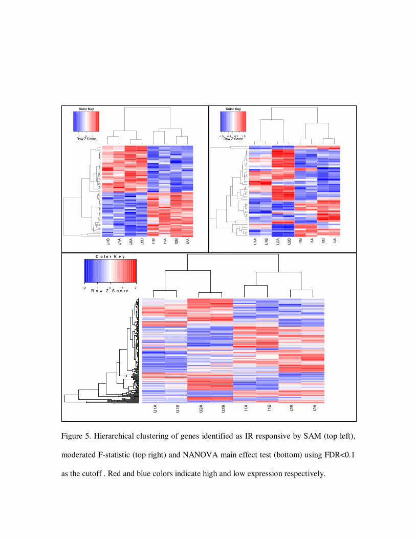
Figure 5. Hierarchical clustering of genes identified as IR responsive by SAM (top left),

moderated F-statistic (top right) and NANOVA main effect test (bottom) using FDR<0.1

as the cutoff . Red and blue colors indicate high and low expression respectively.

U1B

U1A

U2A

U2B

I1B

I1A

I2B

I2A

-1 0 1Row Z-Score

Color Key

U1A

U1B

U2A

U2B

I1B

I1A

I2B

I2A

-1.5 -0.5 0.5 1.5Row Z-Score

Color Key

U1A

U1B

U2A

U2B

I1A

I1B

I2B

I2A

- 2 - 1 0 1 2R o w Z - S c o r e

C o l o r K e y

1 2 3 4 5 6

45

67

8

AF006492_g_at

Log

2-e

xp

ressio

n

1 2 3 4 5 6

89

10

11

Msa.613.0_f_at

Lo

g2-e

xpre

ssio

n

Figure 6. Expression patterns of two probe sets from 1C (upper panel) and 2C (lower

panel). Each point represents an averaged log2-expression value over replicates. Solid

lines: 129SvEv mice; dotted lines: C57BL/6 mice. X-axis: 1: amygdala; 2: cerebellum; 3:

cortex; 4: entorhinal cortex; 5: hippocampus; 6: midbrain

A.A

g.1

A.A

g.2

A.C

b.1

A.

Cb

.2A

.Cx

.1A

.Cx

.2A

.Ec

.1A

.Ec

.2A

.Hp

.1A

.Hp

.2A

.Mb

.1A

.Mb

.2B

.Ag

.1B

.Ag

.2B

.Cb

.1B

. C

b.2

B.C

x.1

B.C

x.2

B.E

c.1

B.E

c.2

B.H

p.1

B.H

p.2

B.M

b.1

B.M

b.2

Tagln3Sf3b5Txnl4Cpne1Aldh7a1LOC241572---Stxbp2Kif5bOTTMUSG00000010673Nkiras1Pebp1HmgcrPebp1LOC100045967Acp1Stk25Cd99EG433058CyctKrt14---5730494N06RikPrdx2PamHnrpcLOC100044227Cap1Ocel11810037I17Rik

-3.0 -2.7 -2.4 -2.1 -1.7 -1.4 -1.1 -0.8 -0.5 -0.2 0.2 0.5 0.8 1.1 1.4 1.7 2.1 2.4 2.7 3.0

Figure 7. Heat map of 3C . Array labels: A for 129SvEv, B for C57BL/6. 1 and 2 are two

replicates. Ag : amygdala; Cb: cerebellum; Cx: cortex; Ec: entorhinal cortex; Hp:

hippocampus; Mb: midbrain. Red and blue colors indicate high and low expression

respectively.

A.A

g.1

A.A

g.2

A.C

b.1

A.

Cb

.2A

.Cx

.1A

.Cx

.2A

.Ec.1

A.E

c.2

A.H

p.1

A.H

p.2

A.M

b.1

A.M

b.2

B.A

g.1

B.A

g.2

B.C

b.1

B.

Cb

.2B

.Cx

.1B

.Cx

.2B

.Ec.1

B.E

c.2

B.H

p.1

B.H

p.2

B.M

b.1

B.M

b.2

Abcf2Foxa2Ephb6Cdk2Hpcal1Klkb1---Mcm42700097O09RikStxbp1GabrdCxcl1Ryr1AgtrapNrkMdfiNeurod1LOC100045404 /// Sycp1Polr2aZfp289Bmp1Pvalb---St8sia5Ptpn22Epb4.1---Kcnj12H2-D1---4833441D16RikGabra6Pcp2Gdf10Ebf1Car8Cry1D7Ertd183eSlc27a2LOC100047506 /// Pbx3LOC240657 /// Psmc1Decr1Cxcr4AarsAcvr2bGm98Spp1Bag3Eps8Otud7bSlc6a8Syt2Atp2a24-SepCfl2Enpp2Col9a3Tinf2Mtap4C80068MogAnlnGsnKctd9Lef1RenbpSrebf1Dlk1AgtAmotl2Itih3SncgLOC100045304 /// NefhVamp1Dlk1AgtAvpNr2f2Zfp777Sars2FrzbNpr3Nr4a2Fezf2Myo5bMapk3LOC100046302 /// Pdia6Ddx25LorOprl1Fhod3Pde1aMef2cStx1aRprmSox11NfybPrss12Matn2Cdh13Pak3---Phlda11110008P14RikLin7bWwc1Lmo4NrgnPtk2bFoxg1Lmo7Mef2cCrip2Slc30a3Arf3ArhgdigNgefSstD430019H16RikCx3cl1Cx3cl1Tac1Magel2EfsPtprePopdc3CebpdKsr1Npy2rKlk8Sae2PrkccAtp1a1

-3.0 -2.7 -2.4 -2.1 -1.7 -1.4 -1.1 -0.8 -0.5 -0.2 0.2 0.5 0.8 1.1 1.4 1.7 2.1 2.4 2.7 3.0

Figure 8. Heat map of 134 filtered probe sets of 4C . Array labels: A for 129SvEv, B for

C57BL/6. 1 and 2 are two replicates. Ag : amygdale;Cb: cerebellum; Cx: cortex; Ec:

entorhinal cortex; Hp: hippocampus; Mb: midbrain. Red and blue colors indicate high

and low expression respectively.