THE FLORIDA STATE UNIVERSITY

COLLEGE OF ARTS AND SCIENCES

A BLOCK INCREMENTAL ALGORITHM FOR

COMPUTING DOMINANT SINGULAR SUBSPACES

By

CHRISTOPHER G. BAKER

A Thesis submitted to theDepartment of Computer Science

in partial fulfillment of therequirements for the degree of

Master of Science

Degree Awarded:Summer Semester, 2004

The members of the Committee approve the Thesis of Christopher G. Baker defended

on April 19, 2004.

Kyle GallivanProfessor Directing Thesis

Anuj SrivastavaCommittee Member

Robert van EngelenCommittee Member

The Office of Graduate Studies has verified and approved the above named committee members.

ii

This thesis is dedicated, even when I am not:

to my parents, who forbade me to attend law school,

and to Kelly, for supporting me throughout the entire process.I promise I will pay off one day.

iii

ACKNOWLEDGMENTS

I would first like to acknowledge my gratitude to my committee members, Professor Anuj

Srivastava and Professor Robert van Engelen. They served willingly for a student who was

not always willing to work.

I am obliged to Dr. Younes Chahlaoui, for many discussions and much advice regarding

this thesis. I am grateful as well to Dr. Pierre-Antoine Absil, for his advisements on writing.

Were it not for these two men, the French translation of my thesis would not have been

possible.

To the many people at the FSU School of Computational Science and Information

Technology, where this research was conducted: the systems group kept things working;

Mimi Burbank provided neverending help in typesetting this thesis; and I received much

assistance and encouragement from members of the CSIT faculty, in particular Professor

Gordon Erlebacher, Professor Yousuff Hussaini, and Professor David Banks.

I would do a great disservice to overlook the contributions of Professor Paul Van Dooren.

I owe much to his counsel. He imparted unto me much insight into the nature of the methods

discussed in this thesis. His suggestions and criticisms are the fiber of this document, and I

proudly count him as a de facto advisor on this thesis.

Finally, I wish to thank my advisor, Professor Kyle Gallivan. Without his support—

academic, technical, and of course, financial—this work would not have been possible.

His ability to explain complicated topics and to illustrate subtle points is unmatched.

Perhaps more remarkable is his willingness to do so. I am indebted to him for inpsiring

my appreciation and interest for the field of numerical linear algebra, just as he attempts to

do with everyone he meets. He is a professor in the greatest sense of the word.

This research was partially supported by the National Science Foundation under grant

CCR-9912415.

iv

TABLE OF CONTENTS

List of Tables . . . . . . . . . . . . . . . . . . . . . . . . . . . . . . . . . . . . . . vii

List of Figures . . . . . . . . . . . . . . . . . . . . . . . . . . . . . . . . . . . . . viii

Abstract . . . . . . . . . . . . . . . . . . . . . . . . . . . . . . . . . . . . . . . . ix

1. INTRODUCTION . . . . . . . . . . . . . . . . . . . . . . . . . . . . . . . . . 1

2. CURRENT METHODS . . . . . . . . . . . . . . . . . . . . . . . . . . . . . . 72.1 UDV methods . . . . . . . . . . . . . . . . . . . . . . . . . . . . . . . . . 7

2.1.1 GES-based methods . . . . . . . . . . . . . . . . . . . . . . . . . . 72.1.2 Sequential Karhunen-Loeve . . . . . . . . . . . . . . . . . . . . . . 9

2.2 QRW methods . . . . . . . . . . . . . . . . . . . . . . . . . . . . . . . . 10

3. A BLOCK INCREMENTAL ALGORITHM . . . . . . . . . . . . . . . . . . . 123.1 A Generic Separation Factorization . . . . . . . . . . . . . . . . . . . . . 123.2 An Incremental Method . . . . . . . . . . . . . . . . . . . . . . . . . . . 133.3 Implementing the Incremental SVD . . . . . . . . . . . . . . . . . . . . . 16

3.3.1 Eigenspace Update Algorithm . . . . . . . . . . . . . . . . . . . . . 173.3.2 Sequential Karhunen-Loeve . . . . . . . . . . . . . . . . . . . . . . 183.3.3 Incremental QRW . . . . . . . . . . . . . . . . . . . . . . . . . . . 193.3.4 Generic Incremental Algorithm . . . . . . . . . . . . . . . . . . . . 21

3.3.4.1 GenInc - Dominant Space Construction . . . . . . . . . . . 223.3.4.2 GenInc - Dominated Space Construction . . . . . . . . . . . 24

3.3.5 Operation Count Comparison . . . . . . . . . . . . . . . . . . . . . 273.4 Computing the Singular Vectors . . . . . . . . . . . . . . . . . . . . . . . 273.5 Summary . . . . . . . . . . . . . . . . . . . . . . . . . . . . . . . . . . . 29

4. ALGORITHM PERFORMANCE COMPARISON . . . . . . . . . . . . . . . 314.1 Primitive Analysis . . . . . . . . . . . . . . . . . . . . . . . . . . . . . . 314.2 Methodology . . . . . . . . . . . . . . . . . . . . . . . . . . . . . . . . . 33

4.2.1 Test Data . . . . . . . . . . . . . . . . . . . . . . . . . . . . . . . . 334.2.2 Test Libraries . . . . . . . . . . . . . . . . . . . . . . . . . . . . . . 34

4.3 Results and Analysis . . . . . . . . . . . . . . . . . . . . . . . . . . . . . 354.4 Summary . . . . . . . . . . . . . . . . . . . . . . . . . . . . . . . . . . . 39

v

5. BOUNDS ON ACCURACY . . . . . . . . . . . . . . . . . . . . . . . . . . . . 425.1 A Priori Bounds . . . . . . . . . . . . . . . . . . . . . . . . . . . . . . . 435.2 A Posteriori Bounds . . . . . . . . . . . . . . . . . . . . . . . . . . . . . 485.3 Improving Bound Approximations . . . . . . . . . . . . . . . . . . . . . . 535.4 Summary . . . . . . . . . . . . . . . . . . . . . . . . . . . . . . . . . . . 57

6. IMPROVING COMPUTED BASES . . . . . . . . . . . . . . . . . . . . . . . 586.1 Pivoting . . . . . . . . . . . . . . . . . . . . . . . . . . . . . . . . . . . . 596.2 Echoing . . . . . . . . . . . . . . . . . . . . . . . . . . . . . . . . . . . . 616.3 Partial Correction . . . . . . . . . . . . . . . . . . . . . . . . . . . . . . 656.4 Summary . . . . . . . . . . . . . . . . . . . . . . . . . . . . . . . . . . . 69

7. CONCLUSION . . . . . . . . . . . . . . . . . . . . . . . . . . . . . . . . . . . 707.1 Future Work . . . . . . . . . . . . . . . . . . . . . . . . . . . . . . . . . 71

APPENDICES . . . . . . . . . . . . . . . . . . . . . . . . . . . . . . . . . . . . . 72

A. Proof of the Complete Decomposition . . . . . . . . . . . . . . . . . . . . . . 72

B. On WY-Representations of Structured Householder Factorizations . . . . . . . 75

C. Testing Specifications . . . . . . . . . . . . . . . . . . . . . . . . . . . . . . . 80

REFERENCES . . . . . . . . . . . . . . . . . . . . . . . . . . . . . . . . . . . . . 81

BIOGRAPHICAL SKETCH . . . . . . . . . . . . . . . . . . . . . . . . . . . . . 83

vi

LIST OF TABLES

3.1 Computational and memory costs of the block algorithms. . . . . . . . . . . 27

3.2 Complexity of implementations for different block size scenarios, for two-sidedalgorithms. . . . . . . . . . . . . . . . . . . . . . . . . . . . . . . . . . . . . 30

4.1 Cost of algorithms in terms of primitive. (·)∗ represents a decrease incomplexity of the GenInc over the SKL-LR, while (·)† represents an increasein complexity of the GenInc over the SKL-LR. . . . . . . . . . . . . . . . . . 32

5.1 Predicted and computed angles (in degrees) between computed subspace andexact singular subspace, for the left (θ) and right (φ) computed singularspaces, for the 1-D flow field dataset, with k = 5 and l = 1. . . . . . . . . . . 52

5.2 Singular value error and approximate bound for the 1-D flow field data set,with k = 5, l = 1, σ6 = 1.3688e + 03. . . . . . . . . . . . . . . . . . . . . . . 52

5.3 Predicted and computed angles (in degrees) between computed subspace andexact singular subspace, for the left (θ) and right (φ) computed singularspaces, for the 1-D flow field dataset, with k = 5 and l = {1, 5}. . . . . . . . 54

5.4 Singular value error and approximate bound for the 1-D flow field data set,with k = 5, l = 5. . . . . . . . . . . . . . . . . . . . . . . . . . . . . . . . . . 55

5.5 Predicted and computed angles (in degrees) between computed subspace andexact singular subspace, for the left (θ) and right (φ) computed singularspaces, for the 1-D flow field dataset, with k = 5(+1) and l = {1, 5}. . . . . . 56

5.6 Singular value error and approximate bound for the 1-D flow field data set,with k = 5(+1), l = {1, 5}. . . . . . . . . . . . . . . . . . . . . . . . . . . . . 56

6.1 Performance (with respect to subspace error in degrees) for pivoting and non-pivoting incremental algorithms for random A, K = 4. . . . . . . . . . . . . 61

6.2 Partial Completion compared against a one-pass incremental method, withand without Echoing, for the C20-720 data with K = 5. . . . . . . . . . . . . 69

vii

LIST OF FIGURES

3.1 The structure of the expand step. . . . . . . . . . . . . . . . . . . . . . . . . 14

3.2 The result of the deflate step. . . . . . . . . . . . . . . . . . . . . . . . . . . 15

3.3 The notching effect of Tu on U1, with ki = 3, di = 3. . . . . . . . . . . . . . . 23

3.4 The notching effect of Su on U2, with ki = 3, di = 3. . . . . . . . . . . . . . . 25

4.1 Performance of primitives and algorithms with ATLAS library. . . . . . . . . 36

4.2 Performance of primitives and algorithms with SUNPERF library. . . . . . . 37

4.3 Performance of primitives and algorithms with Netlib library. . . . . . . . . . 40

4.4 Runtime ratios of primitives (TRMM/GEMM) and algorithms (GenInc/SKL-LR)for different libraries. . . . . . . . . . . . . . . . . . . . . . . . . . . . . . . . 41

5.1 (a) The error in representation (‖A − QfRfWTf ‖/‖A‖2) and (b) final rank

of factorization (kf ) when running the incremental algorithm with increasingblock sizes l. . . . . . . . . . . . . . . . . . . . . . . . . . . . . . . . . . . . . 47

5.2 The effect of a larger block on µ and µ for the 1-D flow field data set, withk = 5 (numbers relative to ‖A‖2). . . . . . . . . . . . . . . . . . . . . . . . . 53

6.1 Angles between true and computed subspaces in degrees illustrates improve-ment from echoing, for the full ORL dataset with K = 5. Red is θk and blueis φk. . . . . . . . . . . . . . . . . . . . . . . . . . . . . . . . . . . . . . . . . 64

viii

ABSTRACT

This thesis presents and evaluates a generic algorithm for incrementally computing the

dominant singular subspaces of a matrix. The relationship between the generality of the

results and the necessary computation is explored, and it is shown that more efficient

computation can be obtained by relaxing the algebraic constraints on the factoriation. The

performance of this method, both numerical and computational, is discussed in terms of the

algorithmic parameters, such as block size and acceptance threshhold. Bounds on the error

are presented along with a posteriori approximations of these bounds. Finally, a group of

methods are proposed which iteratively improve the accuracy of computed results and the

quality of the bounds.

ix

CHAPTER 1

INTRODUCTION

The Singular Value Decomposition (SVD) is one of the most useful matrix decompositions,

both analytically and numerically. The SVD is related to the eigenvalue decomposition of

a matrix. The eigenvalue decomposition for a symmetric matrix B ∈ Rn×n is B = QΛQT ,

where Q is an n× n orthogonal matrix and Λ is an n× n diagonal real matrix.

For a non-symmetric or non-square matrix A ∈ Rm×n, such a decomposition cannot exist.

The SVD provides an analog. Given a matrix A ∈ Rm×n, m ≥ n, the SVD of A is:

A = U

[Σ0

]V T ,

where U and V are m×m and n× n orthogonal matrices, respectively, and Σ is a diagonal

matrix whose elements σ1, . . . , σn are real, non-negative and non-increasing. The σi are the

singular values of A, and the columns of U and V are the left and right singular vectors of

A, respectively. Often times, the SVD is abbreviated to ignore the right-most columns of

U corresponding to the zero matrix below Σ. This is referred to in the literature as a thin

SVD [1] or a singular value factorization [2]. The thin SVD is written as A = UΣV T , where

U now denotes an m × n matrix with orthonormal columns, and Σ and V are the same as

above.

The existence of the SVD of a matrix can be derived from the eigenvalue decomposition.

Consider the matrix B = AT A ∈ Rn×n. B is symmetric and therefore has real eigenvalues

and an eigenvalue decomposition B = V ΛV T . Assuming that A is full rank and constructing

a matrix U as follows

U = AV Λ−1/2,

is easily shown to give the SVD of A:

A = UΛ1/2V T = UΣV T .

1

It should also be noted that the columns of U are the eigenvectors of the matrix AAT .

One illustration of the meaning of the SVD is to note that the orthogonal transformation

V applied to the columns of A yields a new matrix, AV = UΣ, with orthogonal columns

of non-increasing norm. It is clear then that each column vi of V is, under A, sent in the

direction ui with magnitude σi. Therefore, for any vector b =∑n

i=1 βivi,

Ab = A

n∑i=1

βivi

=n∑

i=1

(βiσi)ui.

The subspace spanned by the left singular vectors of A is called the left singular subspace

of A. Similarly, the subspace spanned by the right singular vectors of A is called the right

singular subspace of A. Given k ≤ n, the singular vectors associated with the largest k

singular values of A are the rank-k dominant singular vectors. The subspaces associated

with the rank-k dominant singular vectors are the rank-k dominant singular subspaces.

Consider the first k columns of U and V (Uk and Vk), along with the diagonal matrix

containing the first k singular values (Σk). There are four optimality statements that can be

made regarding the matrices Uk, Σk, and Vk:

1. ‖A− UkΣkVTk ‖2 is minimal over all m× n matrices of rank ≤ k.

2. ‖AT A− VkΣ2kV

Tk ‖2 is minimal over all n× n symmetric matrices of rank ≤ k.

3. ‖AAT − UkΣ2kU

Tk ‖2 is minimal over all m×m symmetric matrices of rank ≤ k.

4. trace(UTk AAT Uk) is maximal over isometries of rank ≤ k.

One commonly used technique for dimensionality reduction of large data sets is Principal

Component Analysis (PCA). Given a set of random variables, the goal of PCA is to determine

a coordinate system such that the variances of any projection of the data set lie on the axes.

These axes are the principal components. Stated more formally, assume that the column

vectors of the matrix A each contain samples of the m random variables. The goal is to

find an isometry P so that B = P T A with the constraint that the covariance cov(B) of B is

2

diagonal with maximum trace. It follows that

cov(B) = E[BBT ]

= E[P T AAT P ]

= P T E[AAT ]P.

Assuming that the mean of the columns of A is zero, the isometry P which maximizes the

trace of cov(B) is Uk, a result of optimality Statement 4.

These vectors (principal components) can be used to project the data onto a lower

dimensional space under which the variance is maximized and uncorrelated, allowing for

more efficient analysis of the data. This technique has been used successfully for many

problems in computer vision, such as face and handwriting recognition.

Another technique, related to PCA, is that of the Karhunen-Loeve Transform (KLT).

The KLT involves computing a low-rank subspace (the K-L basis) under which A is best

approximated. This subspace is the dominant left singular subspace of A, and can be derived

from optimality Statement 2 or 3. KLT has been successfully employed in image/signal

coding and compression applications.

Another application of the SVD is that of the Proper Orthogonal Decomposition (POD).

POD seeks to produce an orthonormal basis which captures the dominant behavior of a large-

scale dynamical system based on observations of the system’s state over time. Known also as

the Empirical Eigenfunction Decomposition [3], this technique is motivated by interpreting

the matrix A as a time series of discrete approximations to a function on a spatial domain.

The dominant SVD can then be interpreted as follows, with

• Uk are a discrete approximation to the spatial eigenfunctions of the function represented

by the columns of A, known as the characteristic eddies [4],

• ΣV Tk are the k coefficients that are used in the linear combination of the eigenfunctions

to approximate each column of A.

A consequence of optimality Statement 1, using Uk, Σk, and Vk minimizes the discrete

energy norm difference between the function represented by the columns of A and the rank-

k factorization UkΣkVTk .

Sirovich [5] introduced the methods of snapshots to efficiently produce this basis. Given a

dynamical system, the method of snapshots saves instantaneous solutions of the system (the

3

snapshots) produced via a direct numerical simulation. The snapshots may be spaced across

time and/or system parameters. The SVD of these snapshots then provides an orthonormal

basis that approximates the eigenfunctions of the system.

This orthonormal basis can be used for multiple purposes. One use is compression, by

producing a low-rank factorization of the snapshots to reduce storage. Another technique

is to use the coordinates of the snapshots in this lower-dimensional space to interpolate

between the snapshots, giving solutions of the system at other time steps or for other system

parameters. A third use combines POD with the Galerkin projection technique to produce a

reduced-order model of the system. This reduced-order model evolves in a lower dimensional

space than the original system, allowing it to be used in real-time and/or memory-constrained

scenarios. Each solution of the reduced-order system is then represented in original state-

space using the orthonormal basis produced by the POD.

A common trait among these applications–PCA and POD–is the size of the data. For

the computer vision cases, the matrix A contains a column for each image, with the images

usually being very large. In the case of the POD, each column of A may represent a snapshot

of a flow field. These applications usually lead to a matrix that has many more rows than

columns. It is matrices of this type that are of interest in this thesis, and it is assumed

throughout this thesis that m � n, unless stated otherwise.

For such a matrix, there are methods which can greatly increase the efficiency of the SVD

computation. The R-SVD [1], instead of computing the SVD of the matrix A directly, first

computes a QR factorization of A:

A = QR.

From this, an SVD of the n × n matrix R can be computed using a variety of methods,

yielding the SVD of A as follows:

A = QR

= Q(UΣV T )

= (QU)ΣV T

= UΣV T .

To compute the R-SVD of A requires approximately 6mn2 +O(n3), and 4mn2 +2mnk +

O(n3) to produce only k left singular vectors. This is compared to 14mn2 + O(n3) for the

4

Golub-Reinsch SVD of A. This is clearly more efficient for matrices with many more rows

than columns.

Another method is to compute the SVD via the eigendecomposition of AT A, as suggested

by the derivation of the SVD given earlier. The eigenvalue decomposition of AT A gives

AT A = V ΛV T , so that

(AV )T (AV ) = Λ = ΣT Σ.

This method requires mn2 operations to form AT A and 2mnk + O(n3) to compute the first

k columns of U = AV T Σ−11 . However, obtaining the SVD via AT A is more sensitive to

rounding errors than working directly with A.

The methods discussed require knowing A in its entirety. They are typically referred to

as batch methods because they require that all of A is available to perform the SVD. In some

scenarios, such as when producing snapshots for a POD-based method, the columns of A will

be produced incrementally. It is advantageous to perform the computation as the columns of

A become available, instead of waiting until all columns of A are available before doing any

computation, thereby hiding some of the latency in producing the columns. Another case is

when the SVD of a matrix must be updated by appending some number of columns. This is

typical when performing PCA on a growing database. Applications with this property are

common, and include document retrieval, active recognition, and signal processing.

These characteristics on the availability of A have given rise to a class of incremental

methods. Given the SVD of a matrix A = UΣV T , the goal is to compute the SVD of the

related matrix A+ =[A P

]. Incremental (or recursive) methods are thus named because

they update the current SVD using the new columns, instead of computing the updated SVD

from scratch. These methods do this in a manner which is more efficient than the O(mn2)

algorithmic complexity incurred at each step using a batch method.

Just as with the batch methods, the classical incremental methods produce a full SVD

of A. However, for many of the applications discussed thus far, only the dominant singular

vectors and values of A are required. Furthermore, for large matrices A, with m � n, even

the thin SVD of A (requiring O(mn) memory) may be too large and the cost (O(mn2)) may

be too high. There may not be enough memory available for the SVD of A. Furthermore,

an extreme memory hierarchy may favor only an incremental access to the columns of A,

while penalizing (or prohibiting) writes to the distant memory.

These constraints, coupled with the need to only compute the dominant singular vectors

5

and values of A, prompted the formulation of a class of low-rank, incremental algorithms.

These methods track a low-rank representation of A based on the SVD. As a new group

of columns of A become available, this low-rank representation is updated. Then the part

of this updated factorization corresponding to the weaker singular vectors and values is

truncated. In this manner, the dominant singular subspaces of the matrix A can be tracked,

in an incremental fashion, requiring a fraction of the memory and computation needed to

compute the full SVD of A.

In Chapter 2, this thesis reviews the current methods for incrementally computing the

dominant singular subspaces. Chapter 3 describes a generic algorithm which unifies the

current methods. This new presentation gives insight into the nature of the problem of

incrementally computing the dominant singular subspaces of a matrix. Based on this insight,

a novel implementation is proposed that is more efficient than previous methods, and the

increased efficiency is illustrated empirically in Chapter 4.

These low-rank incremental algorithms produce only approximations to the dominant

singular subspaces of A. Chapter 5 discusses the sources of error in these approximations and

revisits the attempts by previous authors to bound this error. Those works are considered in

light of the current presentation of the algorithm, and the effect of algorithmic parameters

upon the computed results is explored. Chapter 6 explores methods for correcting the

subspaces computed by the incremental algorithm, when a second pass through the data

matrix A from column 1 to column n is allowed. Three methods are described, and each is

evaluated empirically. Finally, a summary of this thesis and a discussion of future work is

given in Chapter 7.

6

CHAPTER 2

CURRENT METHODS

This section discusses three methods from the literature to incrementally update the

dominant singular subspaces of a matrix A. The methods are divided into categories,

characterized by the updating technique and the form of the results at the end of each

step.

The UDV methods are characterized by the production of a factorization in SVD-like

form, consisting of two orthonormal bases and a non-negative diagonal matrix. The QRW

methods produce orthonormal bases for the singular subspaces along with a small, square

matrix. This matrix contains the current singular values, along with rotations that transform

the two bases to the singular bases.

2.1 UDV methods

In some applications, it is not enough to have bases for the dominant singular subspaces. A

basis for a subspace defines an essentially unique coordinate system, so that when comparing

two different objects, the same basis must be used to compute their coordinates. Therefore,

many applications require the left and right singular bases, those bases composed of ordered

left and right singular vectors. The methods described below compute approximations to

the dominant singular vectors and values of A at each step.

2.1.1 GES-based methods

In [6], Gu and Eisenstat propose a stable and fast algorithm for updating the SVD when

appending a single column or row to a matrix with a known SVD. The topic of their paper

is the production of an updated complete SVD, and does not concern the tracking of the

7

dominant space. However, the work is relevant as the foundation for other algorithms that

track only the dominant subspaces.

The kernel step in their algorithm is the efficient tridiagonalization of a “broken

arrowhead” matrix, having the form:

B =

[Σi z

ρ

]=

σ1 ζ1

. . ....

σk ζn

ρ

= WΣi+1QT ,

where W, Σi+1, Q ∈ R(i+1)×(i+1). Their algorithm is capable of computing the SVD of B in

O(i2) computations instead of the O(i3) computations required for a dense SVD. This is

done stably and efficiently by relating the SVD of the structured matrix to a function of a

special form, that admits efficient evaluation using the fast multipole method.

Chandrasekaran et al. [7, 8] propose an algorithm for tracking the dominant singular

subspace and singular values, called the Eigenspace Update Algorithm (EUA). Given an

approximation to the dominant SVD of the first i columns of A, A(1:i) ≈ UiΣiVTi , and the

next column, a, the EUA updates the factors as follows:

a⊥ = (I − UiUTi )a

u = a⊥/‖a⊥‖2

T =

[Σi UT

i a0 uT a

]= W Σi+1Q

T

Ui+1 =[

Ui u]W

Vi+1 =

[Vi 00 1

]Q.

Ui+1, Σi+1, and V Ti+1 are obtained by truncating the least significant singular values and

vectors from Ui+1, Σi+1, and V Ti+1, respectively. All vectors corresponding to the singular

values lower than some user-specified threshold, ε, are truncated. The EUA was the first

algorithm to adaptively track the dominant subspace.

The SVD of T can be obtained either via a standard dense SVD algorithm or by utilizing

the GES method mentioned above. The GES produces Ui+1, Vi+1, and Σi+1 in O(mk).

However, the overhead of this method makes it worthwhile only for large values k. Otherwise,

a dense SVD of T produces Ui+1, Vi+1, and Σi+1 in O(mk2). Note also that the arrowhead-

based method is only possible if a single row or column is used to update the SVD at

8

each step. Later methods allow more efficient inclusion of multiple rows or columns. The

formation of the intermediate matrices in the algorithms discussed is rich in computation

involving block matrix operations, taking advantage of the memory hierarchy of modern

machines. Furthermore, it will be shown later that bringing in multiple columns at a time

can yield better numerical performance. The UDV and QRW methods in the following

sections utilize block algorithms to reap these benefits.

2.1.2 Sequential Karhunen-Loeve

In [9], Levy and Lindenbaum propose an approach for incrementally computing the a basis

for the dominant left singular subspace. Their algorithm, the Sequential Karhunen-Loeve

(SKL), allows a block of columns to be brought in on each step, and the authors recommend

a block size which minimizes the overall complexity of the algorithm, assuming the number of

columns per block is under user control. While the work of Levy and Lindenbaum concerns

finding the KL basis (the dominant left singular basis), their technique can be modified to

compute a low-rank factorization of A without dramatically affecting the performance.

The update is analogous to that of the EUA. The incoming vectors P (of size m × l)

are separated into components, UT P and P T P , contained in and orthogonal to the current

dominant space:

B′ =[

B P]

=[

U P] [

D UT P

0 P T P

] [V T 00 I

]= U ′D′V ′T .

Next, the SVD of D′ is computed,

D′ = UDV T .

The SVD of B′ clearly is

B′ = U ′D′V ′T = (U ′U)D(V ′V )T .

Finally, the rank of the dominant space is determined, based on a user specified threshold

and the noise space is truncated.

The SVD of D′ is computed in a negligible O(k3) per step, but the formation of the

dominant part of U ′U requires 2m(k + l)k. Combined with the formation of U ′ from U and

P in 4m(k+l)l, this yields a total complexity of 2mnk2+3lk+2l2

lto process the entire matrix A.

It is shown that, assuming a fixed size for k, a block size l can be determined that minimizes

9

the total operations. They show that the value of l = k√2

yields a minimal operation count of

(4√

2+6)mnk ≈ 12mnk. The authors make qualitative claims about the convergence of the

approximation under certain assumptions, but they give neither quantitative explanation

nor rigorous analysis.

In [10], Brand proposes an algorithm similar to that of Levy and Lindenbaum. By using

an update identical to that of the SKL, followed by a dense SVD of the k× k middle matrix

and a matrix multiplication against the large current approximate basis, the algorithm has a

larger leading coefficient than is necessary. Brand’s contribution is the ability of his algorithm

to handle missing or uncertain values in the input data, a feature not pursued in this thesis.

2.2 QRW methods

The defining characteristic of the UDV-based algorithms is that they produce at each step an

approximation to the singular bases, instead of some other bases for the dominant singular

subspaces. However, if the goal of the algorithm is to track the dominant subspace, then all

that is required is to separate the dominant subspace from the noise subspace at each step,

so that the basis for the noise space can be truncated. This is the technique that the QRW

methods use to their computational advantage.

In [11], Chahlaoui, Gallivan and Van Dooren propose an algorithm for tracking the dom-

inant singular subspace. Their Incremental QRW (IQRW) algorithm produces approximate

bases for the dominant left singular subspace in 8mnk + O(nk3) operations. It can also

produce both bases for the left and right dominant singular subspaces in 10mnk + O(nk3)

operations.

This efficiency over the earlier algorithms is a result of a more efficient kernel step. On

each step, the next column of A (denoted by a) is used to update the dominant basis.

Given a current low-rank factorization, QRW T , the step begins by updating the existing

transformation in a Gram-Schmidt-type procedure identical to those used in the previously

discussed algorithms:

10

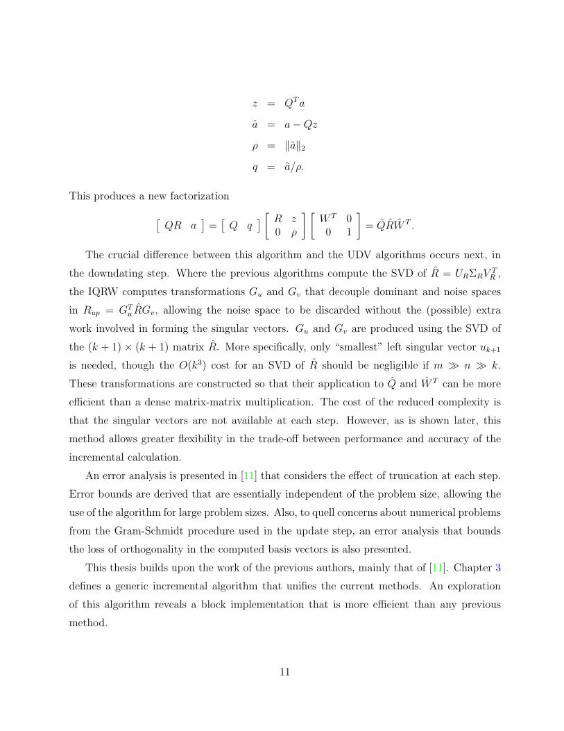
z = QT a

a = a−Qz

ρ = ‖a‖2

q = a/ρ.

This produces a new factorization[QR a

]=

[Q q

] [R z0 ρ

] [W T 00 1

]= QRW T .

The crucial difference between this algorithm and the UDV algorithms occurs next, in

the downdating step. Where the previous algorithms compute the SVD of R = URΣRV TR ,

the IQRW computes transformations Gu and Gv that decouple dominant and noise spaces

in Rup = GTu RGv, allowing the noise space to be discarded without the (possible) extra

work involved in forming the singular vectors. Gu and Gv are produced using the SVD of

the (k + 1) × (k + 1) matrix R. More specifically, only “smallest” left singular vector uk+1

is needed, though the O(k3) cost for an SVD of R should be negligible if m � n � k.

These transformations are constructed so that their application to Q and W T can be more

efficient than a dense matrix-matrix multiplication. The cost of the reduced complexity is

that the singular vectors are not available at each step. However, as is shown later, this

method allows greater flexibility in the trade-off between performance and accuracy of the

incremental calculation.

An error analysis is presented in [11] that considers the effect of truncation at each step.

Error bounds are derived that are essentially independent of the problem size, allowing the

use of the algorithm for large problem sizes. Also, to quell concerns about numerical problems

from the Gram-Schmidt procedure used in the update step, an error analysis that bounds

the loss of orthogonality in the computed basis vectors is also presented.

This thesis builds upon the work of the previous authors, mainly that of [11]. Chapter 3

defines a generic incremental algorithm that unifies the current methods. An exploration

of this algorithm reveals a block implementation that is more efficient than any previous

method.

11

CHAPTER 3

A BLOCK INCREMENTAL ALGORITHM

This chapter outlines a generic block, incremental technique for estimating the dominant left

and right singular subspaces of a matrix. The technique is flexible, in that it can be adapted

to the specific requirements of the application, e.g. left space bases only, left and right space

bases, singular vectors, etc. Such variants are discussed in this chapter, and their efficiency

is characterized using their operation count.

Section 3.1 introduces a generic technique for isolating the dominant subspaces of a matrix

from the dominated subspaces. Section 3.2 describes an algorithm for incrementally tracking

the dominant left and/or right singular subspaces of a matrix, using the technique introduced

in Section 3.1. Section 3.3 discusses implementations of this generic algorithm, and analyzes

the relationship between the operation count of the algorithm and the computational results.

Furthermore, a new algorithm is proposed which has a lower operation count than existing

methods. Finally, Section 3.4 discusses techniques for obtaining the singular vectors using

methods which do not explicitly produce them.

3.1 A Generic Separation Factorization

Given an m× (k + l) matrix M and its QR factorization,

k+l︷︸︸︷ m−k−l︷︸︸︷M =

[Q1 Q2

] [R0

]= Q1R,

consider the SVD of R and partition it conformally as

R = UΣV T =[

U1 U2

] [Σ1 00 Σ2

] [V1 V2

]T,

12

where U2, Σ2, and V2 contain the smallest l left singular vectors, values and right singular

vectors of R, respectively. Let the orthogonal transformations Gu and Gv be such that they

block diagonalize the singular vectors of R,

GTu U =

[Tu 00 Su

]and GT

v V =

[Tv 00 Sv

]. (3.1)

Applying these transformations to R yields Rnew = GTu RGv. Gu and Gv rotate R to a

coordinate system where its left and right singular bases are block diagonal. It follows that

Rnew has the form

Rnew = GTu RGv = GT

u UΣV T Gv

=

[Tu 00 Su

] [Σ1 00 Σ2

] [T T

v 00 ST

v

]=

[TuΣ1T

Tv 0

0 SuΣ2STv

]. (3.2)

The SVD of the block diagonal matrix Rnew has a block diagonal structure. This gives a

new factorization of M :

M = Q1R = (Q1Gu)(GTu RGv)G

Tv = QRnewGT

v = Q

[TuΣ1T

Tv 0

0 SuΣ2STv

]GT

v ,

whose partitioning identifies bases for the dominant left and right singular subspaces of M

in the first k columns of Q and Gv. It should be noted that Gu is not uniquely defined by

Equation (3.1). This definition admits any Gu whose first k columns are some orthonormal

basis for the dominant left singular subspace of R, and whose last l columns therefore are

some orthonormal basis for the dominated (weaker) left singular subspace of R. This is also

the case, mutatis mutandis, for Gv.

3.2 An Incremental Method

The factorization of the previous section can be used to define a generic method that requires

only one pass through the columns of an m× n matrix A to compute approximate bases for

the left and right dominant singular subspaces. The procedure begins with a QR factorization

of the first k columns of A, denoted A(1:k) = Q0R0, and with the right space basis initialized

to W0 = Ik.

The first expansion step follows with i = 1 and s0 = k, where i refers to the step/iteration

of the algorithm and si = si−1 + li refers to the number of columns of A that have been

13

“processed” after completing step i. The li incoming columns of A, denoted A+ = A(si−1+1:si),

are used to expand Qi−1 and Ri−1 via a Gram-Schmidt procedure:

C = QTi−1A+

A⊥ = A+ −Qi−1QTi−1A+ = A+ −Qi−1C

A⊥ = Q⊥R⊥.

The li× li identity is appended to W Ti−1 to expand the k×si−1 matrix to k+ li×si, producing

a new factorization [Qi−1Ri−1W

Ti−1 A+

]= QRW T , (3.3)

the structure of which is shown in Figure 3.1.

Qi−1 Q⊥

Ri−1 C

R⊥

W Ti−1

Ili = QRW T

Figure 3.1: The structure of the expand step.

Transformations Gu and Gv are constructed to satisfy Equation (3.1). These transfor-

mations are applied to the block triangular matrix R to put it in a block diagonal form that

isolates the dominant singular subspaces from the dominated subspaces, as follows:

QRW T = Q(GuGTu )R(GvG

Tv )W T

= (QGu)(GTu RGv)(G

Tv W T )

= QRW T .

The structure of QRW T is shown in Figure 3.2.

14

Figure 3.1: The structure of the expand step.

“processed” after completing step i. The li incoming columns of A, denoted A+ = A(si−1+1:si),

are used to expand Qi−1 and Ri−1 via a Gram-Schmidt procedure:

C = QTi−1A+

A⊥ = A+ −Qi−1QTi−1A+ = A+ −Qi−1C

A⊥ = Q⊥R⊥.

The li× li identity is appended to W Ti−1 to expand the k×si−1 matrix to k+ li×si, producing

a new factorization [Qi−1Ri−1W

Ti−1 A+

]= QRW T , (3.3)

the structure of which is shown in Figure 3.1.

Transformations Gu and Gv are constructed to satisfy Equation (3.1). These transfor-

mations are applied to the block triangular matrix R to put it in a block diagonal form that

isolates the dominant singular subspaces from the dominated subspaces, as follows:

QRW T = Q(GuGTu )R(GvG

Tv )W T

= (QGu)(GTu RGv)(G

Tv W T )

= QRW T .

The structure of QRW T is shown in Figure 3.2.

14

The dominant singular subspaces for[

Qi−1Ri−1WTi−1 A+

]are contained in the first k

columns of Q and rows of W T . The columns Qi, rows W Ti , and the last columns and rows

in R are truncated to yield Qi, Ri, and W Ti , which are m×k, k×k, and k× si, respectively.

This rank-k factorization is an approximation to the first si columns of A.

Qi Qi

Ri 0

0 Ri

W Ti

W Ti = QRW T

Figure 3.2: The result of the deflate step.

The output at step i includes

• Qi - an approximate basis for the dominant left singular space of A(1:si),

• Wi - an approximate basis for the dominant right singular space of A(1:si), and

• Ri - a k× k matrix whose SVD contains the transformations that rotate Qi and Wi to

the dominant singular vectors. The singular values of Ri are estimates for the singular

values of A(1:si).

Note that after the i-th step, there exists an orthogonal matrix Vi embedding Wi and

relating the first si columns to the current approximation of A and the discarded data up to

this point:

ki︷︸︸︷ si−ki︷︸︸︷ ki︷ ︸︸ ︷ d1︷ ︸︸ ︷ di︷ ︸︸ ︷A(1:si)Vi = A(1:si)

[Wi W⊥

i

]=

[QiRi Q1R1 · · · QiRi

].

More specifically, after the final step f of the algorithm, there exists Vf such that

A(1:sf )Vf = A[

Wf W⊥f

]=

[QfRf Q1R1 · · · QfRf

],

15

Figure 3.2: The result of the deflate step.

The dominant singular subspaces for[

Qi−1Ri−1WTi−1 A+

]are contained in the first k

columns of Q and rows of W T . The columns Qi, rows W Ti , and the last columns and rows

in R are truncated to yield Qi, Ri, and W Ti , which are m× k, k× k, and k× si, respectively.

This rank-k factorization is an approximation to the first si columns of A.

The output at step i includes

• Qi - an approximate basis for the dominant left singular space of A(1:si),

• Wi - an approximate basis for the dominant right singular space of A(1:si), and

• Ri - a k× k matrix whose SVD contains the transformations that rotate Qi and Wi to

the dominant singular vectors. The singular values of Ri are estimates for the singular

values of A(1:si).

Note that after the i-th step, there exists an orthogonal matrix Vi embedding Wi and

relating the first si columns to the current approximation of A and the discarded data up to

this point:

ki︷︸︸︷ si−ki︷︸︸︷ ki︷ ︸︸ ︷ d1︷ ︸︸ ︷ di︷ ︸︸ ︷A(1:si)Vi = A(1:si)

[Wi W⊥

i

]=

[QiRi Q1R1 · · · QiRi

].

More specifically, after the final step f of the algorithm, there exists Vf such that

A(1:sf )Vf = A[

Wf W⊥f

]=

[QfRf Q1R1 · · · Qf Rf

],

15

yielding the following additive decomposition:

A = QfRfWTf +

[Q1R1 . . . Qf Rf

]W⊥

f

T.

This property is proven in Appendix A and is used to construct bounds [12] on the error of

the computed factorization.

3.3 Implementing the Incremental SVD

In this section, the current methods for incrementally computing dominant singular sub-

spaces are described in terms of the generic algorithmic framework of Section 3.2. The

computation in this framework can be divided into three steps:

1. The Gram-Schmidt expansion of Q, R, and W . This step is identical across all methods

and requires 4mkl to compute the coordinates of A+ onto Q and the residual A⊥, and

4ml2 to compute an orthonormal basis for A⊥, the cost per step is 4ml(k + l). The

total cost over nl

steps is 4mn(k + l), one of two cost-dominant steps in each method.

2. Each method constructs Gu and Gv based on the SVD of R. Whether the SVD is

computed using classical methods (as in the SKL and IQRW) or accelerated methods

(using the GES as in the EUA) determines the complexity. All methods discussed in

this thesis depend on the ability to perform this step in at most O(k3) computations,

which is negligible when k � n � m.

3. Finally, the computation of Gu and Gv varies across methods, as does the application

of these transformations to Q and W . The methods are distinguished by the form of

computation in Steps 2 and 3.

The following subsections describe the approach taken by each method to implement

Steps 2 and 3. The methods discussed are the EUA, SKL, and IQRW algorithms, and

the Generic Incremental algorithm (GenInc). Complexity is discussed in terms of operation

count, with some discussion of memory requirements and the exploitation of a memory

hierarchy.

16

3.3.1 Eigenspace Update Algorithm

Recall that in the generic framework, the end products of each step are bases for the dominant

singular subspaces and a low-rank matrix encoding the singular values and the rotations

necessary to transforms the current bases to the singular bases. The EUA, however, does

more than that. Instead of producing the factorization in a QBW form, EUA outputs in

a UDV form. The bases output by this method are the singular bases, i.e., those bases

composed of the ordered singular vectors.

This is accomplished by the choice of the transformations Gu and Gv. For Gu and Gv,

the EUA uses the singular vectors of R, Gu = U and Gv = V . These choices clearly satisfy

the conditions in Equation (3.1), as

GTu U =

[UT

1

UT2

] [U1 U2

]=

[Iki

00 Idi

]and

GTv V =

[V T

1

V T2

] [V1 V2

]=

[Iki

00 Idi

].

By using the singular vectors for Gu and Gv, this method puts Rnew into a diagonal form,

such that the Qi and Wi produced at each step are approximations to the dominant singular

bases. That is, the method produces the singular value decomposition of a matrix that is

near to A(1:si).

The EUA uses the Gram-Schmidt expansion described in Section 3.2. The matrix R is a

broken arrowhead matrix, having the form

R =

σ1 ζ1

. . ....

σk ζn

ρ

= UΣV T .

For the SVD of the R, the authors propose two different methods. The first utilizes the Gu

and Eisenstat SVD (GES) [6]. By employing this method, the singular values of R can be

computed and Gu and Gv can be applied in O(mk log22 ε) (where ε is the machine precision).

With a complexity of over (52)2mk per update (for a machine with 64-bit IEEE floats),

this complexity is prohibitive except when k is large. Furthermore, GES requires a broken

arrowhead matrix, restricting this approach to a scalar (li = 1) algorithm.

If the GES method is not used, however, then the computation of QGu and WGv require

2mk2 and 2sik2, respectively. Passing through all n columns of A, along with the Gram-

17

Schmidt update at each step, requires 8mnk + 2mnk2 + O(n2k2) + O(nk3). For this number

of computations, the R-SVD could have been used to produce the exact SVD of A.

In terms of operation count, the EUA is only interesting in the cases where the

efficiency of GES can be realized. Even in these cases, where the overall computation is

O(mnk)+O(n2k)+O(nk2), the leading order constant (at least log22 ε) exceeds those of other

methods. As for the non-GES, matrix multiply method, the O(mnk2) + O(n2k2) + O(nk3)

is much slower than that of other methods, which only grow linearly with k in the dominant

terms.

3.3.2 Sequential Karhunen-Loeve

The SKL method proceeds in a manner similar to the EUA. Using the Gram-Schmidt

expansion described in the generic framework, the SKL method expands the current bases

for the dominant singular subspaces to reflect the incoming columns A+.

The SKL method also uses the singular vectors U and V for the transformations Gu and

Gv. Again, these specific transformations produce not just bases for the dominant singular

subspaces, but the dominant singular bases.

The authors are interested in approximating the Karhunen-Loeve basis (the basis

composed of the dominant left singular vectors). They do not consider the update of the right

singular basis. However, as this thesis is interested in the computation of an approximate

singular value decomposition, the update of the right singular subspace and calculations of

complexity are included (although the added complexity is not significant when m � n). In

the remainder of this thesis when discussing the SKL it is assumed that the right singular

vectors are produced at each step, in addition to the left singular vectors. To make this

explicit, this two-sided version of the of the SKL algorithm is referred to as the SKL-LR.

Producing the singular vectors and values of the ki + li × ki + li matrix R requires

a dense SVD, at O(k3i + l3i ) operations. The matrix multiply QGu, producing only

the first ki columns, requires 2mki(ki + li) operations. Likewise, producing the first ki

columns of WGv requires 2siki(ki + li). Combining this with the effort for the SVD

of R and the Gram-Schmidt expansion, the cost per step of the SKL-LR algorithm is

2m(k2i + 3kili + 2l2i ) + O(k3

i ) + 2siki(ki + li). Fixing ki and li and totaling this over n/l

18

steps of the algorithm, the total cost is

Cskl =∑

i

2m(k2i + 3kili + 2l2i ) + O(k3

i ) + 2si(ki + li)

≈n/l∑i=1

[2m(k2 + 3kl + 2l2) + O(k3) + 2ilk(k + l)

]= 2mn

k2 + 3kl + 2l2

l+ O(

nk3

l) + 2lk(k + l)

n/l∑i=1

i

= 2mnk2 + 3kl + 2l2

l+ O(

nk3

l) +

n2k(k + l)

l.

Neglecting the terms not containing m (appropriate when k � n � m or when only updating

the left basis), the block size l = k/√

2 minimizes the number of floating point operations

performed by the algorithm. Substituting this value of l into the total operation count yields

a complexity of (6 + 4√

2)mnk + (1 +√

2)n2k + O(nk2) ≤ 12mnk + 3n2k + O(nk2).

Note that this linear complexity depends on the ability to choose li = ki√2

at each step.

Many obstacles may prevent this. The SKL-LR algorithm requires m(k + l) memory to hold

Q and mk workspace for the multiplication QGu. If memory is limited, then the size of k

cuts into the available space for l. Also, as in the active recognition scenario, an update

to the dominant singular vectors might be required more often than every ki√2

snapshots, so

that l < k√2. As l approaches 1, the cost for each step approaches 2mk2 + 6mk, with the

cost over the entire matrix approaching 2mnk2 + 6mnk + n2k2 + O(nk3), which is a higher

complexity than computing the leading k singular vectors and values of A using the R-SVD.

3.3.3 Incremental QRW

The Incremental QRW method of Chahlaoui et al. [12] is only described for the scalar case

(l = 1), though the authors allude to a “block” version. A presentation of this block version

is described here.

Using the same Gram-Schmidt update employed by the generic algorithm and the

previously described methods, the authors describe the construction of Gu and Gv. The

transformation Gu is constructed such that

GTu U2 =

[0Idi

],

19

and Gv such that GTu RGv = Rnew is upper triangular. It is easily shown that

RTnew

[0Idi

]=

[0

RT3

]= V2Σ2

where V2 = GTv V2 are the di weaker right eigenvectors of Rnew.

If R is non-singular (as assumed by the authors), and therefore Σ2 is as well, then

V2 =

[0

RT3

]Σ−1

2 and, by its triangularity and orthogonality, V2 =

[0Idi

]. This “transform-

and-triangularize” technique of the IQRW satisfies Equation (3.1). Furthermore, the

resulting factorization of each step contains an upper triangular matrix instead of a dense

block, detailing the source of the name IQRW.

To compute the transformations Gu and Gv at each step, the authors propose two different

methods. In the case where the left and right subspaces are tracked, both QGu and WGv

are computed. Therefore, the applications of Gu and Gv must be as efficient as possible.

The authors present a technique that uses interleaved Givens rotations to build Gu from U2,

while at the same time applying the rotations to R, and building Gv to keep GuR upper

triangular. These rotations are applied to Q and W as they are constructed and applied to

R. To transform U2 to

[0Id

]requires kl + l2/2 rotations. Applying these rotations to Q then

requires 6mkl + 3ml2. Furthermore, each rotation introduces an element of fill-in into the

triangular matrix R, which must be eliminated by Gv. Absorbing these rotations into W

requires 6sikl + 3sil2 flops.

Including Steps 1 and 2 of the generic algorithm, the overall complexity of the two-

sided, Givens-based technique (over n/l steps) is 10mnk + 7mnl + 3n2k + 32n2l + O(n

lk3).

This Givens-based method was proposed to lower the cost of updating the right basis. The

motivation for this construction of Gu and Gv was to minimize the amount of work required

to update the right basis at each step. This is significant when l = 1, the scenario in which

this algorithm was generated, because the update step is performed n times, instead of nl.

For this scenario, the Givens-based IQRW requires only 10mnk + 3n2k + O(nk3).

However, if the right basis is not tracked (and WGv therefore is not needed), the authors

propose a different technique that reduces the cost of the left basis update. By using

Householder reflectors instead of Givens rotations, Gu can be composed of l reflectors of

order k+1 to k+ l. The cost of applying these to Q is 4mkl+2ml2. Restoring GTu R to upper

20

triangular is done via an RQ factorization, of negligible cost. Including Steps 1 and 2, the

complexity of this Householder-based IQRW (over nl

update steps) is 8mnk+6mnl+O(nlk3).

When used in the l = 1 scenario, the complexity becomes 8mnk + O(nk3).

It should be noted that this method of defining Gu and Gv does not succeed when R is

singular. A simple counterexample illustrates this. If U2 =

[0Idi

], then Gu = I, and GT

u R

is still upper triangular. Then Gv also is the identity, and

Rnew = R =

[R1 R2

0 0

].

The dominant and dominated singular subspaces are clearly not separated in this Rnew.

A modification of this transform-and-triangularize method is always successful. Switch

the roles of Gu and Gv, so that

GTv V2 = V2 =

[0Idi

]and Gu restores RGv to upper triangular. This is the a well-known technique for subspace

tracking described in Chapter 5 of [2]. Using this method, it can be shown that the dominant

and dominated subspaces are decoupled in the product Rnew. However, there is a drawback

to constructing Gu in this fashion. In the cases where m � n (the assumption made in [12]

and this thesis), the goal is to minimize the number of operations on the large, m × k + l

matrix Q. When Gu is constructed, as in the IQRW, based on U2, it can be applied more

efficiently than when Gu is constructed to retriangularize RGv.

3.3.4 Generic Incremental Algorithm

The separation technique described in Section 3.2 is the heart of the generic incremental

SVD. It requires only that the first k columns of Gu are a basis for the dominant singular

subspace of R and that the last d columns of Gu are a basis for the dominated singular

subspace. The EUA and the SKL-LR both compose Gu specifically from the basis composed

of the left singular vectors. This is done in order to produce a UDV factorization at every

step.

Alternatively, the IQRW uses bases for the dominant subspaces which leave GTu RGv in

an upper triangular form. The upper triangular middle matrix offers advantages over an

unstructured square matrix in that the storage requirement is cut in half, the system formed

21

by the matrix is easily solved, and operations such as tridiagonalization and multiplication

can be performed more efficiently. While the middle matrix R is only k × k, the above

operations can become significant as k becomes large, especially as R exceeds cache size.

This section describes an implementation, the Generic Incremental Algorithm (GenInc).

The GenInc is similar to the IQRW, in that it focuses on lowering the operation count via

a special construction of Gu and Gv. The GenInc has two variants, each which is preferable

under different parametric circumstances. These variants are described in the following

subsection.

3.3.4.1 GenInc - Dominant Space Construction

Recall that the generic block algorithm requires that orthogonal transformations Gu and Gv

be constructed which block diagonalize the left and right singular vectors of R:

GTu U =

[Tu 00 Su

]and GT

v V =

[Tv 00 Sv

].

This is equivalent to constructing transformations Gu and Gv such that

GTu U1T

Tu =

[Iki

0

]and GT

v V1TTv =

[Iki

0

](3.4)

or

GTu U2S

Tu =

[0Idi

]and GT

v V2STv =

[0Idi

]. (3.5)

This means that the Tu and Su transformations can be specified to rotate the singular bases

to other bases that are more computationally friendly. Since only the first ki columns of

the products QGu and WGv are to be kept, it is intuitive that working with Equation (3.4)

may be more computationally promising. As the construction of Tu and Gu, based on U1,

is analogous to that of Tv and Gv, based instead on V1, the process is described below for

the left transformations only, with the right side transformations proceeding in the same

manner, mutatis mutandis.

The remaining issue is how much structure can be exploited in G1 = U1TTu . Since only

the first ki columns of QGu, QGu

[Iki

0]T

= QG1 are needed and G1 must be a basis for

the dominant left singular subspace, there is a limit on the number of zeroes that can be

introduced with T Tu . Taking the ki + di × ki matrix U1, construct an orthogonal matrix Tu

that transforms U1 to an upper-trapezoidal matrix, “notching” the lower left-hand corner

22

G1 = U1TTu =

υ1,1 υ1,2 υ1,3

υ2,1 υ2,2 υ2,3

υ3,1 υ3,2 υ3,3

υ4,1 υ4,2 υ4,3

υ5,1 υ5,2 υ5,3

υ6,1 υ6,2 υ6,3

T Tu =

η1,1 η1,2 η1,3

η2,1 η2,2 η2,3

η3,1 η3,2 η3,3

η4,1 η4,2 η4,3

0 η5,2 η5,3

0 0 η6,3

Figure 3.3: The notching effect of Tu on U1, with ki = 3, di = 3.

as illustrated in Figure 3.3. This is done by computing the RQ factorization U1 = G1Tu.

G1 = U1TTu is the upper trapezoidal matrix shown in Figure 3.3

It follows that G1 is of the form

G1 =

[BU

],

where B is an di × ki dense block and U is a ki × ki upper-triangular matrix. Any Gu

embedding G1 as

Gu =[

G1 G⊥1

]clearly satisfies Equation (3.4), for any G⊥

1 that completes the space.

Computing the first ki columns of QGu then consists of the following:

QGu

[Iki

0

]= Q

[G1 G⊥

1

] [Iki

0

]= QG1

= Q

[BU

]= Q(1:di)B + Q(di+1:di+ki)U.

This computation requires 2mdiki for the product Q(1:di)B and mk2i for the product

Q(di+1:di+ki)U (because of the triangularity of U), for a total of mki(2di + ki) to produce

the first ki columns of QGu. Similarly, the cost to produce the first ki columns of WGv is

siki(2di + ki).

The total cost per step, including the Gram-Schmidt update and the SVD of R, is

4mli(ki−1 + li) + mki(2di + ki) + siki(2di + ki) + O(k3i + d3

i ). Assuming fixed values of ki and

23

li on each step, the total cost of the algorithm over the entire matrix becomes

Cds =∑

i

[4mli(ki−1 + li) + mki(2di + ki) + siki(2di + ki) + O(k3

i + d3i )

]≈

n/l∑i=1

[4ml(k + l) + mk(2l + k) + ilk(2l + k) + O(k3 + l3)

]= 6mnk + 4mnl +

mnk2

l+ O(

nk3

l+ nl2) + lk(2l + k)

n/l∑i=1

i

= 6mnk + 4mnl +mnk2

l+ O(

nk3

l+ nl2) +

n2(2kl + k2)

2l.

Fixing m, n, and k and neglecting terms not containing m, the block size l = k2

minimizes

the overall complexity of the algorithm, yielding a complexity of 10mnk + 2n2k + O(nk2).

The memory requirement is just m(k + l) for the matrix Q. Note that the dominant space

construction requires no work space. This is because the triangular matrix multiplication

to form QG1 can be performed in-situ, and the rectangular matrix multiplication can be

accumulated in this same space.

3.3.4.2 GenInc - Dominated Space Construction

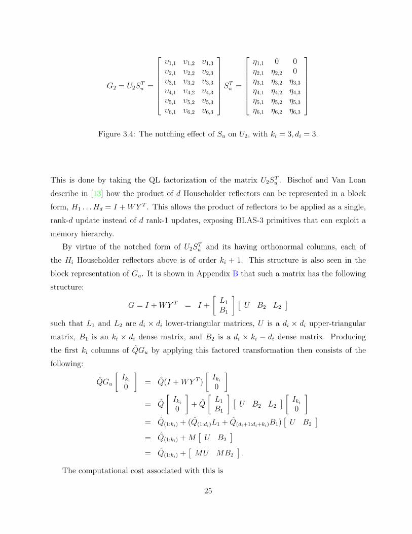
It is worthwhile to investigate the result of forming Gu based on Equation (3.5). Recall that

in this scenario, Gu is defined such that

GTu U2S

Tu =

[0Idi

].

This requires that the last di columns of Gu are equal to U2STu . First a transformation ST

u

that notches the upper-right hand corner of U2 as shown in Figure 3.4 is constructed.

Any Gu of the form

Gu =[

G⊥2 G2

]satisfies Equation (3.5), for some completion of the basis, G⊥

2 . However, unlike before, the

completed basis G⊥2 is needed, because the first ki columns of QGu are given by the quantity

QG⊥2 .

In this case, Gu can be obtained directly from Equation (3.5) using Householder reflectors,

such that

GTu (U2S

Tu ) = HT

di. . . HT

1 (U2STu ) =

[0Idi

]. (3.6)

24

G2 = U2STu =

υ1,1 υ1,2 υ1,3

υ2,1 υ2,2 υ2,3

υ3,1 υ3,2 υ3,3

υ4,1 υ4,2 υ4,3

υ5,1 υ5,2 υ5,3

υ6,1 υ6,2 υ6,3

STu =

η1,1 0 0η2,1 η2,2 0η3,1 η3,2 η3,3

η4,1 η4,2 η4,3

η5,1 η5,2 η5,3

η6,1 η6,2 η6,3

Figure 3.4: The notching effect of Su on U2, with ki = 3, di = 3.

This is done by taking the QL factorization of the matrix U2STu . Bischof and Van Loan

describe in [13] how the product of d Householder reflectors can be represented in a block

form, H1 . . . Hd = I + WY T . This allows the product of reflectors to be applied as a single,

rank-d update instead of d rank-1 updates, exposing BLAS-3 primitives that can exploit a

memory hierarchy.

By virtue of the notched form of U2STu and its having orthonormal columns, each of

the Hi Householder reflectors above is of order ki + 1. This structure is also seen in the

block representation of Gu. It is shown in Appendix B that such a matrix has the following

structure:

G = I + WY T = I +

[L1

B1

] [U B2 L2

]such that L1 and L2 are di × di lower-triangular matrices, U is a di × di upper-triangular

matrix, B1 is an ki × di dense matrix, and B2 is a di × ki − di dense matrix. Producing

the first ki columns of QGu by applying this factored transformation then consists of the

following:

QGu

[Iki

0

]= Q(I + WY T )

[Iki

0

]= Q

[Iki

0

]+ Q

[L1

B1

] [U B2 L2

] [Iki

0

]= Q(1:ki) + (Q(1:di)L1 + Q(di+1:di+ki)B1)

[U B2

]= Q(1:ki) + M

[U B2

]= Q(1:ki) +

[MU MB2

].

The computational cost associated with this is

25

• md2i for the triangular matrix multiplication of Q(1:di)L1,

• 2mkidi for the matrix multiplication of Q(di+1:di+ki)B1,

• md2i for the triangular matrix multiplication of M = Q(1:di)L1 + Q(di+1:di+ki)B1 by U ,

and

• 2m(ki − di)di for the matrix multiplication of MB2.

The total cost for the factored update of the first ki columns of Q then is 4mkidi.

Note that this update is linear in m, ki and di, as opposed to the update using the Gu,

which had a complexity mki(2di + ki). The “dominant space” Gu is simpler to compute,

requiring only the notching of U1 and two matrix multiplications. However, the more

complicated “dominated space” Gu has a lower complexity when l ≤ k2.

Including the Gram-Schmidt update and the SVD of R, the cost per step when using the

dominated space construction of Gu and Gv is 4mli(ki + li) + 4mkidi + 4sikidi + O(k3i + d3

i ).

Assuming maximum values for ki and li on each step, the total cost of the algorithm is

Cws =∑

i

[4mli(ki + li) + 4mkidi + 4sikidi + O(k3

i + d3i )

]≈

n/l∑i=1

[4ml(k + l) + 4mkl + 4ilkl + O(k3 + l3)

]= 8mnk + 4mnl + O(

nk3

l+ nl2) + 4kl2

n/l∑i=1

i

= 8mnk + 4mnl + O(nk3

l+ nl2) + 2n2k.

If 1 ≤ l ≤ k2, the motivating case, then this can be bounded:

Cws = 8mnk + 4mnl + O(nk3

l+ nl2) + 2n2k

≤ 8mnk + 2mnk + O(nk3 + nk2) + 2n2k

= 10mnk + 2n2k + O(nk3).

In this case, the cost related to computing the SVD of R is more significant than

in the dominant space construction. This is a consequence of the smaller block sizes

li, requiring that more steps of the algorithm be performed in order to pass through A.

26

Furthermore, unlike in the dominant space construction, this dominated space construction

requires some working space, in addition to the m(k + l) space required to store the

matrix Q. This work space requires ml memory, and is necessary to store the matrix

M = Q(1:di)L1 + Q(di+1:di+ki)B1.

3.3.5 Operation Count Comparison

The operation counts for the two GenInc implementations are lower than that of previous

methods. Noting Table 3.1, the SKL-LR algorithm, has a total complexity of approximately

12mnk. The Gram-Schmidt update and SVD of R are identical for both the GenInc and

SKL-LR algorithms. The only difference is the update of the dominant singular bases. This

imposes a cost of 2mk(k + l) for the SKL-LR algorithm, but only 2mk(k + l)−mk2 for the

dominant space GenInc. Furthermore, when li ≤ k/2, the lower-complexity, dominated space

GenInc may be used, requiring only 4mkl.

Table 3.1: Computational and memory costs of the block algorithms.

Algorithm SKL-LR GenInc (d.s.) GenInc (w.s.)Complexity 12mnk 10mnk ≤ 10mnkWork Space mk none ml

For equivalent values of k and l, the SKL-LR algorithm has a higher operation count than

the GenInc. The only benefit provided by this extra work is that the SKL-LR computes an

approximation to the singular bases, whereas the GenInc provides arbitrary bases for the

dominant singular subspaces. This shortcoming of the GenInc can be addressed and is the

subject of the next section.

3.4 Computing the Singular Vectors

The efficiency of the GenInc method arises from the ability to use less expensive computa-

tional primitives (triangular matrix multiplies instead of general matrix multiplies) because

of special structure imposed on the transformations used to update the bases at each step.

The SKL-LR method, on the other hand, always outputs a basis composed of the dominant

singular vectors. Whether or not this is necessary varies across applications. If the basis is

27

to be used for a low-rank factorization of the data,

A = UΣV T ≈ UkΣkVTk = QkRkW

Tk

then the choice of basis is irrelevant Also, if the basis is to be used to compute or apply a

projector matrix for the dominant subspace, then the choice of basis does not matter, as

the projector is unique for a subspace. However, if the application calls for computing the

coordinates of some vector(s) with respect to a specific basis, then that specific basis must

be used, explicitly or implicitly. It is the case in many image processing applications that the

user wishes to have the coordinates of some vector(s) with respect to the dominant singular

basis. In this case, the basis output by the GenInc is not satisfactory.

However, as the basis Qi output by the GenInc at each step represents the same space

as does the basis Ui output by the SKL-LR algorithm, then it follows that there is a ki × ki

rotation matrix relating the two:

Ui = QiX.

This transformation X is given by the SVD of Ri = UrΣrVTr , as

UiΣiVTi = QiRiW

Ti = (QiUr)Σr(VrWi)

T .

In the case of the Dominant Space GenInc, the matrix X is readily available. Recall from

Equation (3.2) that the SVD of Ri (the ki × ki principal submatrix of R) is given by

Ri = TuΣT Tv

where Tu and T Tv are the matrices used to notch the dominant singular subspaces of R at

step i. In addition to producing the matrices Qi, Ri, and Vi at each step, GenInc can also

output the transformations Tu and Tv, which rotate Qi and Wi to the dominant singular

bases Ui and Vi.

Computing the coordinates of some vector b with respect to Ui consists of computing the

coordinates with respect to Qi and using Tu to rotate to the coordinate space defined by Ui,

as follows:

UTi b = (QiTu)

T b = T Tu (QT

i b).

The production of QTi b requires the same number of operations as that of UT

i b, and the

additional rotation by T Tu occurs in ki-space, and is negligible when ki � m. As this

28

rotation matrix is small (ki × ki), the storage space is also negligible compared to the space

required for the m× ki matrix Qi (and even compared to the si × ki matrix Wi).

Unlike the Dominant Space construction, when the GenInc is performed using the

Dominated Space construction of Gu and Gv, the matrices Tu and Tv are not computed.

The matrix Su is used to notch the dominated subspace basis U2, and Gu is constructed to

drive U2STu to

[0 Idi

]T. This is achieved using Householder reflectors, as illustrated in

Equation (3.6). It is nevertheless possible to compute Tu during this step. Recall that Gu is

defined to block-diagonalize U , such that

GTu U = GT

u

[U1 U2

]=

[Tu 00 Su

].

By applying GTu to U1, during or after constructing it from U2S

Tu , Tu can be constructed. If

Tv is also needed, it can be constructed in a similar manner, by applying GTv to V1.

Therefore, the dominant singular bases can be made implicitly available using the GenInc,

at a lower cost than explicitly producing them with the SKL-LR. It should be noted that

when the dominant singular subspaces are explicitly required on every step (e.g., to visualize

the basis vectors), they can still be formed, by rotating the bases Qi and Wi by Tu and Tv,

respectively. The cost for this is high, and in such a case it is recommended to use a method

(such as the SKL-LR) that explicitly produces the singular basis.

In cases where the singular bases are required only occasionally, a hybrid method is the

most efficient. Using such a method, the SKL-LR separation step is used whenever the

explicit singular bases are required, and the less expensive GenInc is otherwise employed.

This results in a savings of computation on the off-steps, at the expense of storing a ki × ki

block matrix instead of just the ki singular values composing Σi at step i.

3.5 Summary

This chapter describes a generic incremental algorithm which unifies previous methods for

incrementally computing the dominant singular subspaces of a matrix. The current methods–

the EUA, SKL-LR, and IQRW algorithms–are shown to fit into this framework. Each of

these methods implements the generic algorithm in order to achieve specific results. A new

method (GenInc) is proposed which achieves a lower operation count by relaxing the criteria

on the computed factorization.

29

Table 3.2 shows the computational complexity of the different implementations of the

generic algorithm, as they relate to the block size. The EUA (using the Gu-Eisenstat SVD)

only exists for a scalar update and has a higher operation count than other algorithms. The

IQRW has a low operation count for a scalar update, but the operation count is not as

competitive for non-trivial block sizes.

Table 3.2: Complexity of implementations for different block size scenarios, for two-sidedalgorithms.

Scenario EUA IQRW SKL-LR GenInc

l fixed - 10mnk + 7mnl 2mnk2

l + 6mnk + 4mnl8mnk + 4mnl (w)

mnk2

l + 6mnk + 4mnl (d)l = 1 (log2

2 ε)mnk 10mnk 2mnk2 + 6mnk 8mnk (w)l optimal - - 12mnk (l = k√

2) 10mnk (l = k

2 ) (d)

The operation count of the SKL-LR method relies on the ability to choose as optimal

the block size. Many things prevent this from being realized. The greatest obstacle to this

is that there may not be storage available to accumulate the optimal number of columns

for an update. This is further complicated by the higher working space requirements of the

SKL-LR (Table 3.1).

These issues are resolved by the introduction of a new algorithm, the GenInc. By

considering a generic formulation of the incremental subspace tracking algorithm and relaxing

some of the constraints imposed by the previous method–triangular storage and the explicit

production of singular vectors–a new method is proposed that has a lower a complexity

than other methods. Two different constructions of the GenInc (the dominant subspace

and dominated subspace constructions) allow the algorithm to maintain a relatively low

operation count, regardless of block size. Proposals are made to extend the GenInc, to

implicitly produce the current dominant singular vectors, in the case that the application

demands them, and a UDV-QBW hybrid algorithm is proposed for cases where an explicit

representation of the singular vectors is required.

The discussion in this chapter centers around the operation count of the algorithms. The

next chapter evaluates the relationship between operation count and run-time performance

of these algorithms, focusing on the performance of individual primitives under different

algorithmic parameters.

30

CHAPTER 4

ALGORITHM PERFORMANCE COMPARISON

Chapter 3 discussed the current low-rank incremental methods in the context of the generic

framework, and presented a novel algorithm based on this framework. The predicted

performance of these methods was discussed in terms of their operation counts. This chapter

explores the circumstances under which performance can be predicted by operation count.

Section 4.1 proposes the questions targeted by the experiments in this chapter. Section 4.2

describes the testing platform. More specifically, the test data is be discussed, along with

the computational libraries that are employed. Lastly, Section 4.3 presents the results of the

performance experiments and analyze them.

4.1 Primitive Analysis

The lower complexity of the GenInc as compared to the SKL-LR is a result of exploiting

the structure of the problem, allowing the use of primitives with lower operation complexity.

More specifically, triangular matrix multiplies (TRMM) as opposed to general matrix multiplies

(GEMM). The complexity, in terms of the operation count for the primitives employed by all

of the algorithms, is given in Table 4.1.

Note that the only differences between the SKL-LR and the GenInc are

• smaller GEMMs for the GenInc,

• two triangular matrix multiplies in the GenInc, not present in the SKL-LR, and

• two very small GEQRFs in the GenInc, not present in the SKL-LR.

The small GEQRF primitives being negligible, the performance difference between the

GenInc and the SKL-LR rests on the performance difference between the TRMM primitive

31

Table 4.1: Cost of algorithms in terms of primitive. (·)∗ represents a decrease in complexityof the GenInc over the SKL-LR, while (·)† represents an increase in complexity of the GenIncover the SKL-LR.

Primitive SKL-LR GenInc (d.s.) GenInc (w.s.)General Matrix k ×m× l k ×m× l k ×m× lMultiply (GEMM) m× k × l m× k × l m× k × l

m× (k + l)× k† m× l × k∗ m× l × k∗

m× l × (k − l)∗

Triangular Matrix m× k × k† m× l × l†

Multiply (TRMM) m× l × l†

SVD (GESVD) (k + l)× (k + l) (k + l)× (k + l) (k + l)× (k + l)QR decomposition m× l m× l m× l

(GEQRF)

and the GEMM primitive. A triangular matrix multiply of order m × k × k requires only

half of the floating point operations as does a general matrix multiply of the same size.

Furthermore, it has the added benefit of being computable in-situ, which cuts in half the

memory footprint and may lead to improved cache performance. For the general matrix

multiply, the multiplication of matrices A and B requires storage space for the output matrix

in addition to the input matrices.

However, if the TRMM is not faster than the GEMM primitive, then the GenInc algorithm

should be slower than the SKL-LR. For a naive implementation of both primitives, the TRMM

should be faster. However, it is sometimes the case when using “optimized” implementations

of these primitives, that some primitives are more optimized than others. More specifically,

commercial implementations of numerical libraries may put more effort into optimizing the

commonly used primitives (such as GEMM and GESVD) and less effort on the less-used primitives

(like TRMM). The result is that the TRMM primitive may actually be slower than the GEMM

primitive in some optimized libraries.

This effect must be always be considered when implementing high performance numerical

algorithms. If the primitives required by the algorithms do not perform well on a given

architecture with a given set of libraries, then it naturally follows that the algorithm does

not perform well (using the given implementation of the prescribed primitives). This is a

well-known and oft-explored fact in the field of high-performance scientific computing. In

32

such a case, the developer has the choice of either using different primitives to implement

the algorithm or of rewriting the primitives to perform better on the target architecture.

The GenInc algorithm requires that a call to the TRMM primitive of order m × k × k

and a GEMM primitive of order m × l × k perform better than a single GEMM primitive of

order m × (k + l) × k. In such cases where the extra time is large enough to cover the

overhead required by the GenInc algorithm (namely, the construction of Gu and Gv), then

the GenInc algorithm outperforms the SKL-LR algorithm. However, if the TRMM primitive

is not significantly faster than the GEMM primitive (for the same inputs), then the GenInc

performs worse, despite its lower operation count.

It is possible to compare the running-time performance of the SKL-LR algorithm against

that of the GenInc algorithm. The performance of the stand-alone primitives (GEMM and

TRMM) constitute the major computational difference between the two and is considered in

the discussion of performance between the two algorithms.

4.2 Methodology

Implementations were created, and timings were collected for three of the algorithms: the

SKL-LR, IQRW, and GenInc. Each was compared against the same baseline. This baseline

is the the low-dimensional R-SVD, computed by

• first performing a rank-n QR factorization,

• followed by an n× n SVD of the triangular factor, and

• finally a matrix multiplication to produce the k left singular vectors from the Q factor

and the left singular vectors of the triangular factor.

The tests were conducted using a Sun Ultra 80, with 1024MB of system memory and

dual UltraSparc-II CPUs. Each CPU has a clock speed of 450MHz and a 4MB L2 cache.

The codes were written in Fortran 95, and compiled to run on a single processor. Further

information regarding compiler version and options can be found in Appendix C.

4.2.1 Test Data

The data used for testing comes from two sources. The actual content of the matrices used

to test is irrelevant; only the dimensions m, n, and k are important. However, these data are

33

representative of some of the application scenarios where sub-space tracking/model-reduction

methods such as the Incremental SVD would be used.

The first dataset is from the Columbia Object Image Library (COIL-20) database. This

database, commonly used for benchmarking performance in image processing applications,

is a collection of images of different objects. The collection contains 72 images each of 20

different objects, for a total of 1440 images. The images for a target object are from varying

angles. Each image is a 128× 128 grayscale, and is represented as a single column vector of

the image matrix A. The performance tests run here considered only the first 10 objects, so

that A has dimensions M = 16384 and N = 720. This dataset is representative of many in

image processing applications, with a fairly large value for M (642, 1282, etc.) and a smaller

(but significant) number of columns.

The second dataset used for performance testing is from a Computational Fluid Dynamics

dataset. Each column of the matrix represents a snapshot of a 3-dimensional flow field, of

dimension 64× 64× 65. The performance tests are run with two versions of the dataset. In

one, only one flow direction of the data set is included, so that the length of each column of

A is m = 64× 64× 65 = 266240. In the other, all three directions of flow are considered, so

that m = 64× 64× 65× 3 = 798720. In both cases, n = 100 snapshots of the flow field are

considered. This dataset is representative of many CFD datasets, with fewer columns than

in image databases like the COIL20, but with columns varying from large (≈ 260, 000) to

very large (≈ 800, 000).

4.2.2 Test Libraries

The different algorithms are tested with a variety of numerical libraries:

• Netlib libraries

• SUNPERF library

• ATLAS library

The Netlib libraries are the BLAS and LAPACK sources from the Netlib repository and

compiled with the Sun compiler. The SUNPERF is a hand-tuned, “optimized” version of

the BLAS and LAPACK routines for use on Sun architectures. The Automatically Tuned

Linear Algebra Software (ATLAS) is a profile-based, self-tuning implementation of often-used

34

routines from the BLAS and LAPACK numerical libraries. ATLAS is primarily intended for

use on machines where no hand-tuned, architecture-specific numerical library is present.

Many architecture vendors provide implementations of the BLAS and LAPACK libraries

specially tuned to the vendor’s platform. Examples include

• AMD’s “AMD Core Math Library” (ACML),

• Intel’s “Intel Math Kernel Library” (IMKL),

• Sun’s “Sun Performance Library” (SUNPERF),

• SGI’s “Scientific Computing Software Library” (SCSL), and

• IBM’s “Engineering and Scientific Subroutine Library” (ESSL).

For users whose platform does not provide tuned libraries, the remaining options are to

download and compile the BLAS and LAPACK libraries from Netlib, or to use ATLAS or

some other self-tuning software package.

4.3 Results and Analysis

The results of the performance testing are shown in Figures 4.1, 4.2, 4.3, and 4.4. The first

three sets of figures show the performance of the two basic primitives (GEMM and TRMM) along

with the performance of all four algorithms: the IQRW, the GenInc, the SKL-LR, and the

R-SVD. This is detailed for each of the three libraries: ATLAS, SUNPERF, and Netlib. The

fourth set of figures show the ratio between the performance the TRMM and GEMM primitives,

along with the ratio of the performance between the GenInc and SKL-LR algorithms.

The first result to note is the improvement in performance of both of the block algorithms

over that of the IQRW. With a complexity of 8mnk and 10mnk (depending on which

method is used) as compared to 12mnk (SKL-LR) and 10mnk (GenInc), the IQRW methods

proposed by Chahlaoui et al. have the lowest operation count of any method. However,

the block methods, exploiting temporal locality and a memory hierarchies, overcome their

increased operation count and yield better running times. Observing Figures 4.1 and 4.2,

this is the case. For the ATLAS and SUNPERF libraries, the level-3 primitives make more

efficient use of the memory hierarchy, allowing the block algorithms to outperform the lower

complexity scalar algorithm.

35

20 40 60 80 100 120 140 160 180 2000

0.05

0.1

0.15

0.2

0.25GEMMTRMM

N

Runti

me

(s)

16000×N primitives - ATLAS

0 50 100 150 200 250 3000

100

200

300

400

500

600

700

800

900

1000IQRWGenIncSKL−LRR−SVD

K

Runti

me

(s)

COIL20-720 - ATLAS

0 5 10 15 20 25 30 35 400

1

2

3

4

5

6

7

8

9GEMMTRMM

N

Runti

me

(s)

266000×N primitives - ATLAS

0 5 10 15 20 25 30 35 400

20

40

60

80

100

120

140IQRWGenIncSKL−LRR−SVD

K

Runti

me

(s)

1-D flow field - ATLAS

0 5 10 15 20 25 30 35 400

5

10

15

20

25

30GEMMTRMM

N

Runti

me

(s)

798000×N primitives - ATLAS

0 5 10 15 20 25 30 35 400

200

400

600

800

1000

1200

1400IQRWGenIncSKL−LR

K

Runti

me

(s)

3-D flow field - ATLAS

Figure 4.1: Performance of primitives and algorithms with ATLAS library.

37

Figure 4.1: Performance of primitives and algorithms with ATLAS library.

36

20 40 60 80 100 120 140 160 180 2000

0.05

0.1

0.15

0.2

0.25GEMMTRMM

N

Runti

me

(s)

16000×N primitives - SUNPERF

0 50 100 150 200 250 3000

100

200

300

400

500

600

700

800

900

1000IQRWGenIncSKL−LRR−SVD

K

Runti

me

(s)

COIL20-720 - SUNPERF

0 5 10 15 20 25 30 35 400

1

2

3

4

5

6

7

8

9GEMMTRMM

N

Runti

me

(s)

266000×N primitives - SUNPERF

0 5 10 15 20 25 30 35 400

20

40

60

80

100

120

140IQRWGenIncSKL−LRR−SVD

K

Runti

me

(s)

1-D flow field - SUNPERF

0 5 10 15 20 25 30 35 400

5

10

15

20

25

30GEMMTRMM

N

Runti

me

(s)

798000×N primitives - SUNPERF

0 5 10 15 20 25 30 35 400

200

400

600

800

1000

1200

1400IQRWGenIncSKL−LR

K

Runti

me

(s)

3-D flow field - SUNPERF

Figure 4.2: Performance of primitives and algorithms with SUNPERF library.

38

Figure 4.2: Performance of primitives and algorithms with SUNPERF library.

37

Note Figure 4.3, the results using the Netlib library. Not only is overall performance

slower than with the two tuned libraries, but the relative performance of the three incremental

algorithms is different. Because the Netlib libraries do not employ blocking to improve

performance of the level-3 primitives, the IQRW algorithm is able to outperform the two

block algorithms.

Next, consider the performance arguments made regarding the two block algorithms.

It was argued previously that, given a TRMM primitive that is more efficient than the GEMM

primitive of the same order, the GenInc should outperform the SKL-LR algorithm.

For the ATLAS library, the performance testing on the primitives show that the TRMM

primitive runs consistently faster than the GEMM primitive (Figure 4.1). The GEMM primitives

show some spiking, both for the ATLAS and SUNPERF libraries, but this is typical of

blocked routines and is predictably absent from the Netlib library.

Considering the algorithm timings using the ATLAS library, the results are straightfor-

ward. In the COIL-20, 1-D CFD, and 3-D CFD scenarios, the TRMM primitives performs on

average 50% better than the GEMM primitive, and it never performs worse. For both the 1-D

and 3-D CFD datasets, the GenInc algorithm has a runtime lower than that of the SKL-LR

algorithm, and in the case of the 3-D CFD dataset, the runtime is much better than would

be predicted by operation counts. Some of this benefit may be because the TRMM primitive is

performed in place, as opposed to the GEMM primitive, which requires work space. This can

lead to a smaller memory footprint and less cache misses, which is more significant in the

3-D CFD scenario, where the data is so much larger than in the 1-D case.

For the COIL image database, however, the GenInc, while out-performing the SKL-LR

for lower values of K, does become more expensive. This trend is not predicted by the

primitive timings for the ATLAS library, where the TRMM stills run in half the of the GEMM.

An explanation for this comes by way of the reduced size of m, relative to n and k. This

reduces the importance of the GEMM and TRMM operations, giving more weight to other work

in the GenInc: the extra QR factorizations used to construct Gu and Gv, in addition to the

smaller step size.

Consider now the performance of the incremental algorithms linked against the SUN-

PERF library (Figure 4.2). First of all, note the lack of improvement in the TRMM primitive

over the GEMM primitive. An operation that should require only half of the runtime, instead

runs as much as 3 and 4 times slower. This translates, for the 1-D CFD scenario, into an

38

increase in runtime for the GenInc, as compared to the SKL-LR. In the case of the 3-D

CFD dataset, even though the TRMM does not perform better than the GEMM, the GenInc

still outperforms the SKL-LR. This is likely a result of the in-situ execution of the TRMM as

compared to the ex-situ execution of the GEMM. As with the ATLAS libraries, this gives the

GenInc an extra benefit over the SKL-LR for this large dataset, and in this case, is able to

make up for a relatively inefficient triangular matrix multiply.

Note the performance of both algorithms using the SUNPERF library for the COIL

dataset. Even though the TRMM primitive out-performs the GEMM, the GenInc under-performs

compared to the SKL-LR. This can be explained, as with the ATLAS implementation, by

the lessened effect of the matrix multiplication primitives, in light of a much smaller m.

4.4 Summary

This chapter illustrates the benefit of both of the block algorithms over a scalar algorithm

and the computational benefit of the GenInc over the SKL-LR algorithm.

The better performance of block update algorithms, in spite of higher operation counts,

over scalar update algorithms comes by utilizing BLAS-3 primitives which exploit a memory

hierarchy. This is clearly illustrated in the experiments presented in Section 4.1. Codes

linked with unoptimized libraries yield runtimes consistent with operation count, resulting

in scalar update algorithms running faster than block update algorithms. However, codes

linked with libraries optimized for a memory hierarchy yield superior performance for block

update algorithms as compared to scalar update algorithms.

Furthermore, this chapter investigates the relative performance of the two block update

algorithms, SKL-LR and GenInc. The increased efficiency of the GenInc is shown to be

tied to the performance of specific primitives. Experiments show that, in the presence of

adequate primitives, the GenInc yields better runtime performance than the SKL-LR.

The next chapter contains a discussion of the source of error in the incremental algorithm,

and it discusses the attempts of previous authors to bound this error. These results are

updated for a block algorithm. Improvements to the bounds are proposed and experiments

are run to validate the discussion.

39

20 40 60 80 100 120 140 160 180 2000

0.5

1

1.5

2

2.5

3

3.5

4

4.5GEMMTRMM

N

Runti

me

(s)

16000×N primitives - Netlib

0 50 100 150 200 250 3000

1000

2000

3000

4000

5000

6000

7000

8000IQRWGenIncSKL−LRR−SVD

K

Runti

me

(s)

COIL20-720 - Netlib

0 5 10 15 20 25 30 35 400

5

10

15

20

25

30

35

40

45GEMMTRMM

N

Runti

me

(s)

266000×N primitives - Netlib

0 5 10 15 20 25 30 35 400

100

200

300

400

500

600

700

800

900IQRWGenIncSKL−LRR−SVD

K

Runti

me

(s)

1-D flow field - Netlib

Figure 4.3: Performance of primitives and algorithms with Netlib library.

41

Figure 4.3: Performance of primitives and algorithms with Netlib library.

40

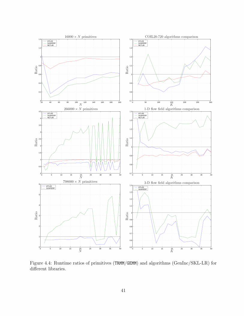
20 40 60 80 100 120 140 160 180 2000

0.2

0.4

0.6

0.8

1

1.2

1.4ATLASSUNPERFNETLIB

N

Rat

io16000×N primitives

0 50 100 150 200 250 3000.7

0.8

0.9

1

1.1

1.2

1.3

1.4ATLASSUNPERFNETLIB

K

Rat

io

COIL20-720 algorithms comparison

0 5 10 15 20 25 30 35 400

0.5

1

1.5

2

2.5

3

3.5

4

4.5ATLASSUNPERFNETLIB

N

Rat

io

266000×N primitives

0 5 10 15 20 25 30 35 400.7

0.8

0.9

1

1.1

1.2

1.3

1.4ATLASSUNPERFNETLIB

K

Rat

io

1-D flow field algorithms comparison

0 5 10 15 20 25 30 35 400

1

2

3

4

5

6ATLASSUNPERF

N

Rat

io

798000×N primitives

0 5 10 15 20 25 30 35 400.5

0.6

0.7

0.8

0.9

1

1.1

1.2

1.3

1.4ATLASSUNPERF

K

Rat

io

3-D flow field algorithms comparison

Figure 4.4: Runtime ratios of primitives (TRMM/GEMM) and algorithms (GenInc/SKL-LR) fordifferent libraries.

42

Figure 4.4: Runtime ratios of primitives (TRMM/GEMM) and algorithms (GenInc/SKL-LR) fordifferent libraries.

41

CHAPTER 5

BOUNDS ON ACCURACY

The computational advantages of the low-rank, incremental algorithms over standard

methods (e.g., R-SVD) do not come without a cost. At each step, the algorithms choose

the optimal low-rank subspace for approximating the local matrix. However, it is a heuristic

argument that these local approximations are globally optimal. Because data truncated from

the factorization is lost forever, the incremental algorithms produce only approximations to

the dominant SVD of the target matrix.

This chapter discusses the efforts of the previous authors to bound the errors in the

incremental algorithm and evaluates the reliability of the error estimates they recommend

in the context of the generic incremental algorithm framework. Two parameters whose

effects on accuracy are examined are the “threshold of acceptance”, δi, and the block size,

li. The threshold δi is used to determine the value for ki+1 at each step i of the algorithm.

That is, after updating the decomposition at step i with li new columns of A, δi is used to

determine the rank of the retained factorization. The block size li has a profound effect both

on the quality of the error estimates and the computational effort required to produce the

decomposition.

The error analyses in this section depend on a theorem introduced in [12] and proven in

Appendix A. This theorem states that after every step of the incremental algorithm, there

exists an orthogonal matrix Vi (embedding Wi) relating the processed columns of A to the

current decomposition and the truncated data, like so:

A(1:si)Vi = A(1:si)

[Wi W⊥

i

]=

[QiRi Q1R1 . . . QiRi

].

This decomposition holds for each step of the algorithm, including the last one. Therefore,

42

there is some orthogonal matrix Vf embedding Wf which transforms the matrix A as follows:

A[Wf W⊥

f

]=

[QfRf Q1R1 . . . Qf Rf

],

so that

A =[QfRf Q1R1 . . . Qf Rf

] [Wf W⊥

f

]T

= QfRfWTf +

[Q1R1 . . . Qf Rf

]W⊥

f

T.

This splits A into two parts: the decomposition produced by the incremental algorithm

and the information truncated at each step from the algorithm. This enables analyses of the

accuracy of the algorithm.

Section 5.1 discusses the error in the low-rank factorization produced by a two-sided

incremental method, as compared to the matrix A. The source of this error is described, as

well as the efforts of previous authors to construct a priori bounds on the error. The effect

of block size on the performance of the algorithm is also studied. Section 5.2 discusses the

a posteriori bounds derived by previous authors on the error in the computed subspaces

and singular values, as well as approximations to these bounds. Previous bounds and

their estimates are reviewed in the context of the generic incremental algorithm. Finally,

Section 5.3 suggests techniques for improving the quality of the bounds and evaluates their

effectiveness.

5.1 A Priori Bounds

In [8], Manjunath et al. concern themselves with two measures of accuracy. With origins in

image processing, each column of A represents an image. The dominant SVD then represents

the ideal rank-k representation of the set of images constituting A (under the 2-norm). They

are therefore concerned with the ability of this low-rank representation to approximate the

individual images. The authors attempt to bound the individual errors in terms of the norm

of the data truncated at each step. This is possible because the data truncated at each step

is bounded in norm by the threshold of acceptance, δi. This is accomplished by choosing

ki+1 (the rank for the next step) so that σki+1+1, . . . , σki+1+di(the singular values of Ri) are

all smaller than δi. For the rest of this discussion, it is assumed that δi is held constant from

step to step (although this is not necessary in practice.) Furthermore, subscripts on ki and

li may at times be dropped for the sake of simplicity.

43

Manjunath et al. propose an argument for the approximating ability of Qi (clarifying

additions by Baker in brackets):

Note that Qi+1 approximates ai+1 [and QiRi] to an accuracy of δ. Similarly Qi

approximates ai to an accuracy of δ. From this it follows that Qi+1 approximates

ai to an accuracy of 2δ. In general, j ≤ i, Qi approximates aj to an accuracy

of (i − j + 1)δ. Therefore if we choose δ to be ε/n we can guarantee that Qn

approximate all the images to an accuracy of ε.

This bound on the representation error of each ai, while correct, is unnecessarily loose.

Recall the decomposition for A(1:i) given above, for a scalar algorithm (l = 1):

A(1:i) = QiRiWTi +

[σ

(1)k+1q1 . . . σ

(i)k+1qi

]W⊥

i

T,

where each σ(i)k+1 ≤ δ. Then, for j ≤ i, the representation error for aj = Aej in QiRiW

Ti is

‖aj −QiRiWTi ej‖2 = ‖A(1:i)ej −QiRiW

Ti ej‖2

=∥∥∥[

σ(1)k+1q1 . . . σ

(i)k+1qi

]W⊥

i

Tej

∥∥∥2

=∥∥∥[

σ(j)k+1qj . . . σ

(i)k+1qi

]∥∥∥2

(5.1)

≤∥∥[

qj . . . qi

]∥∥2

imaxg=j

σ(g)k+1

≤√

i− j + 1δ,

where Equation (5.1) is a result of the trapezoidal structure of W⊥i and its orthonormal

columns (see Appendix A). Therefore, each column of A is approximated to√

nδ by

QnRnWTn , if δ is the threshold for rank-determination used at each step. To guarantee

that all images are approximated to some accuracy ε, δ should be set to ε/√

n.

The second measure of accuracy that Manjunath et al. propose appears in [7]. There,

the authors are concerned with the overall representation error between A and QnRnWTn . It

is proposed in [7] to bound the representation error as follows:

‖A−QnRnWTn ‖2 ≤ nδ.

The authors suggest that this bound is overly conservative and that it should be approxi-

mated by√

nδ. However, using a similar analysis as above, it is easily shown that√

nδ is a

44

bound on the error:

‖A−QnRnWTn ‖2 =

∥∥∥[σ

(1)k+1q1 . . . σ

(n)k+1qn

]W⊥

n

T∥∥∥

2

=∥∥∥[

σ(1)k+1q1 . . . σ

(n)k+1qn

]∥∥∥2

≤√

nδ.

While tighter, this bound is still conservative, and better bounds and approximations are

given later.

Note that both of these bounds improve with a growing block size l. Considering a fixed

block size of l requiring f iterations to pass through all columns of A, the bound on the error

in the approximation is easily revised as:

‖A−QfRfWTf ‖2 =

∥∥∥[Q1R1 . . . Qf Rf

]W⊥

f

T∥∥∥

≤√

fδ

≈√

n− k0

lδ. (5.2)

For a fixed threshold parameter δ, increasing the block size clearly lowers this bound.

However, this only occurs if the allowable rank of the factorization is large enough so that

the discarded singular values are smaller than δ. This may be not be possible due to memory

limitations.

Levy et al. [9] also present an argument that the performance of the algorithm improves

as the block size increases. They describe each column in A as being composed of some

components each of the “true basis vectors” (the dominant k left singular vectors of A)

and of the “noise basis vectors” (the dominated k left singular vectors of A. They propose

that an increased block size allows the algorithm to gather in a single step, more energy

from the “true basis vectors” relative to the “noise basis vectors” (which allegedly do not

have support across multiple columns of A). This allows the “true basis vectors” a better

chance of justifying their existence in the factorization retained by the low-rank incremental

algorithm.

An assumption in this explanation is that each column of A contains some average energy

for each singular vector (dominant and dominated). Another is that each “noise basis vector”

has support in only a single column of A.

45

If the “noise basis vectors” do have support from contiguous columns of A, then increasing

the block size may have the effect of requiring that the rank of the factorization be increased

in order to retain all of the vectors which meet the acceptance threshold. As the rank

of the factorization effects the memory and computational requirements, the rank of the

factorization may be limited by the amount of memory on a computer or by the amount of

time allowed for a single incremental step.

The discussion in [9] suggests that an increased block size allows the incremental

algorithms to better capture the dominant space, even if the rank of the algorithm does not

grow. This statement requires the assumption that each column of A contains the average

energy associated each “true basis vector”. While there is some average energy associated

with each “true basis vector”, the amount of energy in the columns of A associated with each

singular vector may not be uniform across columns. Therefore, the block size of the algorithm

may have to be greatly increased in order for one update to gather more information about

a particular singular vector than would have occurred with a smaller block size.

The following experiment illustrates this point. A matrix A of dimension 1000 × 100

is generated with elements chosen from a standard normal distribution. The incremental

algorithm is applied to this matrix multiple times, with block sizes ranging from 1 to 75,

always initialized with a rank k0 = 5 factorization. Two types of tests are run: “constrained

rank” tests, where the rank of the algorithm is never allowed to grow above 15 (the resulting

rank when run for l = 1); and “free rank” tests, where the rank is determined entirely by the

acceptance threshold δ. This experiment was run multiple times with similarly generated

matrices, and the results were consistent across these runs.

Figure 5.1 shows the results of this experiment. First note that for the rank 15

experiments, the representation error lies between 92% and 94%. However, the ratio

σ16/σ1 = 90% is a lower bound on the norm of the representation error for an approximation

of rank 15.

Noting Figure 5.1(a), in the free rank tests, an increased block size l is met with a

decreased representation error. Figure 5.1(b) shows that as the block size increases, the rank

of the factorization must grow, as predicted above. However, when the rank is not allowed to

grow (in the constrained rank tests), an increase in block size does not result in a significant

decrease in representation error.

This illustrates the argument made above, that the bounds on the error (and the error,

46

0 10 20 30 40 50 60 700.88

0.89

0.9

0.91

0.92

0.93

0.94

0.95Const.Free

Block size - l

‖A−

QfR

fW

T f‖/‖A‖ 2

(a) Error vs. block size

0 10 20 30 40 50 60 7010

15

20

25

30Const.Free

Block size - l

Fin

alra

nk

-k

f

(b) Rank vs. block size

Figure 5.1: (a) The error in representation (‖A − QfRfWTf ‖/‖A‖2) and (b) final rank of

factorization (kf) when running the incremental algorithm with increasing block sizes l.

in practice) decrease as the block size increases. However, this experiment confirms that for

a dynamic rank algorithm based on an absolute threshold of acceptance, the rank of the

algorithm tends to increase with an increasing block size. Furthermore, if the factorization

rank is not allowed to increase, the performance benefits disappear.

Note as well that in the free rank tests, the error does not reduce monotonically

with increasing block size. This is because the optimal block size (in terms of numerical

performance) depends on the support that the dominant singular vectors have in the columns

of A. Without knowing something about this energy (like the “average energy” assumption

in [9]), it is difficult to make rigorous statements about the numerical performance of the

incremental algorithm with respect to block size.

This section outlines the attempts at a priori bounds on the error (‖A−QfRfWfT‖2) by

previous authors, while studying the effect of block size on this error measure. The argument

of Levy et al. [9], that increased block size leads to an improved factorization, is restated and

confirmed with experiments. However, the source of this improvement is shown to be due to

the increased rank of the factorization, itself a result of the increased block size. Block size

alone was shown not to improve performance for a class of randomly generated matrices.

This section also tightens those a priori bounds presented by Manjunath et al. and

updates them for the block algorithm. The following section will present the attempts by

48

Figure 5.1: (a) The error in representation (‖A − QfRfWTf ‖/‖A‖2) and (b) final rank of

factorization (kf ) when running the incremental algorithm with increasing block sizes l.

in practice) decrease as the block size increases. However, this experiment confirms that for

a dynamic rank algorithm based on an absolute threshold of acceptance, the rank of the

algorithm tends to increase with an increasing block size. Furthermore, if the factorization

rank is not allowed to increase, the performance benefits disappear.

Note as well that in the free rank tests, the error does not reduce monotonically

with increasing block size. This is because the optimal block size (in terms of numerical

performance) depends on the support that the dominant singular vectors have in the columns

of A. Without knowing something about this energy (like the “average energy” assumption

in [9]), it is difficult to make rigorous statements about the numerical performance of the

incremental algorithm with respect to block size.

This section outlines the attempts at a priori bounds on the error (‖A−QfRfWfT‖2) by

previous authors, while studying the effect of block size on this error measure. The argument

of Levy et al. [9], that increased block size leads to an improved factorization, is restated and

confirmed with experiments. However, the source of this improvement is shown to be due to

the increased rank of the factorization, itself a result of the increased block size. Block size

alone was shown not to improve performance for a class of randomly generated matrices.

This section also tightens those a priori bounds presented by Manjunath et al. and

47

updates them for the block algorithm. The following section will present the attempts by

previous authors to construct a posteriori bounds on the performance of the incremental

algorithm.

5.2 A Posteriori Bounds

The bound√

n−k0

lδ proposed in [8] is an a priori bound of the representation error,

recommending a value of δ when the tolerable error is known. Because the low-rank

incremental algorithms can produce bad results, it is important to have reliable a posteriori

bounds on the error in the singular subspaces and singular values. Utilizing a posteriori

information about the truncated data allows a tighter bound on this error. In the this

section, the attempts by Chahlaoui et al. [12] to provide tight a posteriori bounds are

revisited for a block algorithm. Their analysis is described and updated for the block case.

Experiments are run to test the prerequisite assumptions of their bounds.

The authors of the IQRW [12] derive bounds on the error in the subspaces produced by

the incremental algorithm. These bounds compare the result of the incremental algorithm

with that of the true SVD. Recall that the work of Chahlaoui et al. described the incremental

algorithm and resulting accuracy analysis only for the scalar case (l = 1).

Their analyses rest on the results of two theorems. The first is the decomposition proven

in Appendix A and has been used throughout this section. Stated again, it proves the

existence of a matrix Vi at each step i of the algorithm satisfying:

A(1:si)Vi = A(1:si)

[Wi W⊥

i

]=

[QiRi Q1R1 . . . QiRi

],

where Qi and Ri are the matrices truncated from the decomposition at step i, and W⊥i is the

orthogonal complement to Wi composed of the truncated Wi and necessary permutations.

Updating their argument shows that each intermediate factorization, produced at step i,

is orthogonally equivalent to a submatrix A(1:si) of A, so that

σ(i)1 ≤ σ1, . . . , σ

(i)ki+li

≤ σki+li

where σ(i)j are the singular values of Ri, and σj are the singular values of A. Then the singular

values that are discarded at each step are all smaller than σ(i)k , the kth

i singular value of A.

48

Furthermore, consider the update at step i:

[QiRi A+

] [W T

i 00 I

]=

[Qi+1 Qi+1

] [Ri+1 0

0 Ri+1

]GT

v

[W T

i 00 I

]⇓[

QiRi A+

]=

[Qi+1 Qi+1

] [Ri+1 0

0 Ri+1

]GT

v (5.3)

The matrix on the right hand side of (5.3) has singular values

σ(i+1)1 , . . . , σ

(i+1)ki+li

.

It also has QiRi as a submatrix, so that

σ(i)1 ≤ σ

(i+1)1 , . . . , σ

(i)ki≤ σ

(i+1)ki

.

The singular values of the computed factorization increase monotonically, with every step of

the algorithm, toward the singular values of A.

It is shown in [12] that bounds can be obtained for the incremental algorithm by relating

the final factorization Qf RfWTf to the matrix A. This is accomplished using the SVD-like

decomposition shown at the end of Appendix A:

A = UMV T =[Qf U Q⊥

f

] [Σ A1,2

0 A2,2

] [Wf V W⊥

f

]T

,

where A2.=

[A1,2

A2,2

]and µ

.= ‖A2‖2.

They apply a theorem from [14], which bounds the distance between the dominant

singular subspaces of

M =

[Σ A1,2

0 A2,2

]and those of

M =

[Σ 00 0

].

Using this theorem, the following bounds are given in [12]:

tan θk ≤µ2

σ2k − 2µ2

if µ ≤ σk√3

(5.4)

tan φk ≤2µ‖A‖2

σ2k − µ2

if µ ≤ 7σ2k

16‖A‖2

, (5.5)

49

where θk and φk are the largest canonical angles between the left and right dominant singular

subspaces of M and M , respectively. These angles also represent the distance between the

dominant subspaces of A and QfRfWTf , so they measure the error in the subspaces computed

by the incremental algorithms.

Furthermore, using these results, [12] derives relative bounds on the errors in the singular

values computed by the incremental algorithm:

|σi − σi| ≤µ2

σi + σi

.

Unfortunately, the matrix A2 is not computed during the low-rank incremental algorithm,

and neither is its norm, µ. To evaluate the bounds, it is necessary to approximate this value.

Consider the matrix A2. Take the matrix

Si =

0Idi

0

,

which selects some QiRi as such:[Q1R1 . . . Qf Rf

]Si = QiRi.

Then the block of columns in A2 corresponding to QiRi has the same 2-norm as Ri:

‖QiRi‖22 = ‖

[Q1R1 . . . Qf Rf

]Si‖2

2

= ‖Qf UA1,2S + Q⊥f A2,2S‖2

2

= ‖Qf UA1,2S + Q⊥f A2,2S‖2

2

= ‖ST AT1,2A1,2S + ST AT

2,2A2,2S‖2

= ‖ST AT2 A2S‖2

= ‖A2S‖22.

Denoting µi as the largest singular value discarded at step i, the 2-norm of A2 can be bounded

above as follows:

‖A2‖22 ≤ µ2 =

f∑i=1

µ2i .

The authors worry that this value may overestimate µ to the point that σ2k − µ2 and

σ2k− 2µ2 become negative. By assuming the truncated vectors to be noise (i.e., uncorrelated

50

and having standard Gaussian distribution), they are able to use a result by Geman [15] to

estimate µ. Defining µ.= maxi µi, each column of A2 then has norm bounded by µ. Geman

shows then that the expected value of µ = ‖A2‖2 has the relation:

µ ≤ µ ≤ cµ, c ≈ 1 +

√n− k0

n≈ 2.

Chahlaoui et al. then recommend approximating µ by µ. They point out that

this approximation has the advantage that, since for each discarded µi it is known that

µi ≤ σk ≤ σ1, and therefore σ2k − µ2 is always non-negative. This allows the proposed

bounds to be approximated as follows:

tan θk ≈ tan θk.=

µ2

σ2k − µ2

,

tan φk ≈ tan φk.=

2µσ1

σ2k − µ2

,

|σi − σi| ≤ µ2

σi + σi

≈ µ2

2σi

.

In [12], Chahlaoui et al. present the results of tests on matrices with randomly

generated elements. These matrices are constructed to have gaps (between σk and σk+1)

of varying size. Their tests show that, even when the necessary assumptions are not met

(Equations (5.4,5.5)), the proven bounds often hold. Furthermore, they illustrate that the

quantity µ is an appropriate approximation for µ, so that the bound approximations do in

practice bound the error in the computed subspaces and singular values.

However, this choice of µ to approximate µ is not always accurate. In the best case,

when the columns of A2 are orthogonal, then µ = µ. However, in the worst case, where the

columns of A2 are coplanar with the same norm (µ), then µ =√

n−k0

lµ. It is always the

case that µ underestimates µ; the extent of this underestimation depends on the directional

information in the discarded columns. The result is that the bounds predicted using µ are

lower than the proven bounds. In some cases they do not actually bound the error in the

computed bases and singular values.

An experiment was run using the 1-D flow field dataset described in Chapter 3, with

k = 5 and l = 1. The resulting errors in the singular values and computed subspaces are

shown in Tables 5.1 and 5.2. In this test, µ = 0.0236, while the approximation is µ = 0.0070

(both relative to the norm of A). This caused the approximate bounds on the error in the

51

computed left subspace and the singular values to be too low, and they do not, in fact, bound

the error in the computed singular values and subspaces.

Table 5.1: Predicted and computed angles (in degrees) between computed subspace andexact singular subspace, for the left (θ) and right (φ) computed singular spaces, for the 1-Dflow field dataset, with k = 5 and l = 1.

θk θk φk φk

k = 5, l = 1 29.1222 5.2962 38.4531 87.8249

Table 5.2: Singular value error and approximate bound for the 1-D flow field data set, withk = 5, l = 1, σ6 = 1.3688e + 03.

i σi σi |σi − σi|/‖A‖2 µ2/(2σi)1 6.4771e+04 6.4771e+04 1.2501e-07 2.4766e-052 3.5980e+03 3.5471e+03 7.8558e-04 4.5224e-043 2.6262e+03 2.5696e+03 8.7311e-04 6.2427e-044 2.0342e+03 1.9387e+03 1.4746e-03 8.2744e-045 1.6909e+03 1.5655e+03 1.9362e-03 1.0247e-03

Note that, while the fifth canonical angle (θ5) between the exact and computed subspace

is not very good, the fifth computed singular value (σ5) matches well with the fifth singular

value (σ5) of A. This is because the gap between σ5 and σ6 is relatively small, meaning that

any linear combination of the fifth and sixth singular vectors can capture nearly as much

energy as the fifth singular vector.

While the performance of the incremental algorithm for this matrix is very good (in

term of the approximation of the singular values), a poor estimation of µ by µ yields poor

approximations to the bounds, causing them to be overly optimistic about the error in

the computed subspaces and singular values. The next section proposes measures to provide

better estimates of the bounds derived by Chahlaoui et al. and demonstrates the effectiveness

of these measures.

52

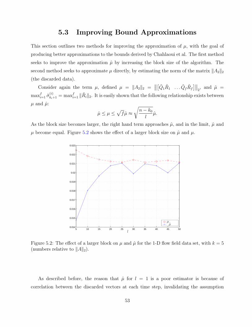
5.3 Improving Bound Approximations

This section outlines two methods for improving the approximation of µ, with the goal of

producing better approximations to the bounds derived by Chahlaoui et al. The first method

seeks to improve the approximation µ by increasing the block size of the algorithm. The

second method seeks to approximate µ directly, by estimating the norm of the matrix ‖A2‖2

(the discarded data).

Consider again the term µ, defined µ = ‖A2‖2 =∥∥[

Q1R1 . . . Qf Rf

]∥∥2, and µ =

maxfi=1 σ

(i)ki+1 = maxf

i=1 ‖Ri‖2. It is easily shown that the following relationship exists between

µ and µ:

µ ≤ µ ≤√

fµ ≈√

n− k0

lµ.

As the block size becomes larger, the right hand term approaches µ, and in the limit, µ and

µ become equal. Figure 5.2 shows the effect of a larger block size on µ and µ.

5.3 Improving Bound Approximations

This section outlines two methods for improving the approximation of µ, with the goal of

producing better approximations to the bounds derived by Chahlaoui et al. The first method

seeks to improve the approximation µ by increasing the block size of the algorithm. The

second method seeks to approximate µ directly, by estimating the norm of the matrix ‖A2‖2

(the discarded data).

Consider again the term µ, defined µ = ‖A2‖2 =∥∥[

Q1R1 . . . QfRf

]∥∥2, and µ =

maxfi=1 σ

(i)ki+1 = maxf

i=1 ‖Ri‖2. It is easily shown that the following relationship exists between

µ and µ:

µ ≤ µ ≤√

fµ ≈√

n− k0

lµ.

As the block size becomes larger, the right hand term approaches µ, and in the limit, µ and

µ become equal. Figure 5.2 shows the effect of a larger block size on µ and µ.

5 10 15 20 25 30 35 40 45 500.014

0.015

0.016

0.017

0.018

0.019

0.02

0.021

0.022

0.023

l

µµ

Figure 5.2: The effect of a larger block on µ and µ for the 1-D flow field data set, with k = 5(numbers relative to ‖A‖2).

As described before, the reason that µ for l = 1 is a poor estimator is because of

correlation between the discarded vectors at each time step, invalidating the assumption

54

Figure 5.2: The effect of a larger block on µ and µ for the 1-D flow field data set, with k = 5(numbers relative to ‖A‖2).

As described before, the reason that µ for l = 1 is a poor estimator is because of

correlation between the discarded vectors at each time step, invalidating the assumption

53

in Geman’s theorem. By increasing the block size from l = 1, more vectors are discarded at

each time step as well. Recall the application of Geman’s theorem to estimate the norm of

the matrix A2. This analysis occurred for a block size of l = 1. For values of l > 1, there are

more columns discarded at each step. Because the data discarded at each step has a known

norm, the matrix A2 can be approximated (for the purpose of finding its norm) by one of

rank n−k0

l, instead of n− k0. If Geman’s theorem is applied to this lower rank matrix, with

a norm denoted by γ, then the result is the following:

µ ≤ γ ≤ cµ, c ≈ 1 +

√n− k

nl≈ 1 +

√1

l.

It is proposed then that the applicability, as well as the quality, of the approximation of µ

by µ should improve as the block size of the algorithm increases. More work is needed to

put this on rigorous analytical ground.

Furthermore, it is intuitive that increasing the block size should improve this estimate.

As the block size is increased to the limit, the algorithm is run with a single incremental step,

which uses the entire remaining part of A to update the initial singular value decomposition.

Then the singular values and vectors computed are in fact the exact (up to finite precision)

values and vectors and µ = µ.

Table 5.3: Predicted and computed angles (in degrees) between computed subspace andexact singular subspace, for the left (θ) and right (φ) computed singular spaces, for the 1-Dflow field dataset, with k = 5 and l = {1, 5}.

µ µ θk θk φk φk

k = 5, l = 1 0.0236 0.0070 29.1222 5.2962 38.4531 87.8249k = 5, l = 5 0.0225 0.0147 21.6580 28.1646 29.4404 89.2113

The resulting improvement in µ yields bounds that are closer to those predicted by [12].

Consider the experiment from Section 5.2: the incremental algorithm applied to the 1-D flow

field dataset with k = 5, but with l = 5. Table 5.3 shows the resulting approximations for

the error in the subspaces, compared against those produced with l = 1. Note that the µ is

a much better approximation for µ. Furthermore, the approximate bounds on the subspace

errors (Table 5.3) and the singular values errors (Table 5.4) now hold.

54

Table 5.4: Singular value error and approximate bound for the 1-D flow field data set, withk = 5, l = 5.

i |σi − σi|/‖A‖2 µ2/(2σi)1 5.6597e-08 1.0866e-042 3.9020e-04 1.9699e-033 4.7044e-04 2.7114e-034 8.3129e-04 3.5539e-035 1.1414e-03 4.3526e-03

Another method for improving the approximate bounds is to directly estimate the value

µ based on the truncated data. Recall the definition of µ:

µ.= ‖A2‖2 =

∥∥[Q1R1 · · · Qf Rf

]∥∥2.

Because the discarded data is large (m× (n− k)), its norm cannot be computed exactly. In

fact, it infeasible even to store this matrix. But, as the individual matrices Qi and Ri may be

produced at each time step, a low-rank incremental algorithm may be used to approximate

the dominant SVD of A2, thereby providing an estimated norm of this matrix. This requires

forming the products QiRi and conducting an incremental algorithm in addition to the main

one. This is expensive and complicated.

An alternative is to perform the incremental algorithm on A as usual, but not keeping

the ki directions dictated by the threshold parameter. Instead, keep the factorization of rank

ki +1, except on the very last step, where this extra tracked direction is dropped, its current

norm being a provably better approximation to µ than the µ proposed by Chahlaoui et al.

This can be shown as follows. Because µ = maxi µi, there is some step i where

µold = µi = σ(i)k+1. When running with rank k + 1, this extra singular value and its

directional information are kept. It was shown earlier that the tracked singular values

increase monotonically, so that when processing the last block of columns of A, the rank is

selected to be k, discarding the extra singular triplet that was being tracked, and obtaining

µ.= σ

(f)k+1 ≥ σ

(i)k+1 = µold.

The benefit of this method is that only one incremental algorithm must be run. By

keeping more than just one extra column, increased performance is expected. To illustrate

this, the previous experiments are run again, with k = 5(+1), for l = 1 and l = 5. For the

55

l = 1 case, µ = 0.0220 and µ = 0.0192 (relative to the norm of A). Note from Tables 5.5 and

5.6 that the errors in the subspaces and singular values fall within the bounds predicted. As

with the increased block size example from before, there is an increase in accuracy due to

the larger tracking rank being able to preserve more information from step to step. However,

there is a much greater increase in the bounds, because of the better approximation of µ by

µ. For comparison with Tables 5.2 and 5.4, the l = 5 test is run again, here with the extra

dimension of tracking. Here µ = 0.0218 is much better approximated by µ = 0.0195, and

the errors in the subspaces and singular values again fall within the approximate bounds.

Table 5.5: Predicted and computed angles (in degrees) between computed subspace andexact singular subspace, for the left (θ) and right (φ) computed singular spaces, for the 1-Dflow field dataset, with k = 5(+1) and l = {1, 5}.

µ µ θk θk φk φk

k = 5(+1), l = 1 0.0220 0.0192 17.9886 55.4335 27.1941 89.6211k = 5(+1), l = 5 0.0218 0.0195 16.3042 56.2570 25.0185 89.6277

Table 5.6: Singular value error and approximate bound for the 1-D flow field data set, withk = 5(+1), l = {1, 5}.

l = 1 l = 5i |σi − σi|/‖A‖2 µ2/(2σi) |σi − σi|/‖A‖2 µ2/(2σi)

1 8.8422e-08 1.8429e-04 7.1704e-08 1.8922e-042 5.7350e-04 3.3522e-03 4.7251e-04 3.4355e-033 5.7055e-04 4.6102e-03 4.7948e-04 4.7226e-034 9.3447e-04 6.0480e-03 7.8978e-04 6.1803e-035 1.1545e-03 7.3862e-03 9.8091e-04 7.5313e-03

Finally, note that the quality of the estimate µ is independent of the quality of the

computed factorization. Consider the matrix A:

A =[Q0R0 Q

(1)1 R

(1)1 . . . Q

(n)1 R

(n)1

],

with Q0, Q1 having orthonormal columns, Q0 ⊥ Q1 and sup(R0) ≥∥∥∥[

R(1)1 . . . R

(n)1

]∥∥∥2

=√

n‖R1‖2. (Superscripts are simply to illustrate repetition and make explicit the count.)

56

The rank of A is clearly just the rank of Q0 plus that of Q1, and Q0 is easily shown to be a

basis for the dominant left singular subspace. If the incremental algorithm is initialized with

Q0, then none of the update steps allow a change in the current subspace, and the algorithm

trivially produces correct bases for the left and right singular subspaces, along with the

singular values of A. Note, however, that when updating each step with Q1R1, the discarded

data has norm ‖R1‖2, so that µ = ‖R1‖2. However, it is clear that µ =√

n‖R1‖2 =√

nµ.

The term µ can be made arbitrarily larger than µ by increasing the number n, so long as

the singular values of R0 are increased to fulfill the hypothetical assumptions.

5.4 Summary

This chapter illustrates some of the errors inherent in the incremental algorithms, due to the

truncation of data at each time step. The attempts by previous authors to a priori bound

these errors are reviewed and updated for the block version of the algorithm. In addition,

these a priori bounds are tightened. The algorithm block size is shown to increase the quality

of the factorization (as it approximates A). However, contrary to arguments made by Levy

et al., this improvement is shown to have its source in an increasing factorization rank.

This chapter also reviews the a posteriori bounds on the error in the computed subspaces

and singular values, derived by Chahlaoui et al. [12]. Their recommended approximations

to these bounds are discussed, and these approximations are shown to sometimes perform

poorly. New techniques are proposed to increase the quality of the approximation of the

µ term, so that the approximations to the error bounds perform more reliably. The first

technique works simply by increasing the block size of the algorithm, showing again the

importance of this parameter with respect to the performance of the algorithm. The second

technique suggests increasing the rank of the factorization until all of the columns have been

processed.

In spite of the improvement in the bound approximations, the a posteriori bounds can

fail, without any indication. This can occur even when the algorithm itself performs very

well. This suggests that, in addition to the approximations for the bounds proposed by

Chahlaoui et al., there is a need for some other mechanism for testing the quality of the

results and signaling when the subspaces might be inaccurate. The next chapter proposes a

set of methods that reveal when improvement in the computation are possible, by exploiting

multiple passes through the matrix A.

57

CHAPTER 6

IMPROVING COMPUTED BASES

One of the motivating factors for the class of incremental algorithms described in this thesis

is that the matrix A is too large to store in local memory. The result is that the matrix

must be stored at a distance (e.g., physical vs. virtual memory, local vs. remote storage,

storage vs. destruction). In such a case, it is not plausible to perform operations on the

matrix (or the current decomposition) that make random accesses reading and writing across

all columns of the matrix, as one would do in a standard block algorithm on a hierarchical

memory. The incremental methods reduce the cost here by processing the matrix in pieces,

taking a group of columns of A, using them to update a low-rank decomposition, and then

discarding this group of columns to make room for the next. Each group of columns of the

matrix is fetched from remote storage to local storage only once, i.e. the matrix is read-only

and any writing is to a significantly smaller amount of storage containing the updated bases

and work space.

As described in Chapter 5, part of the inaccuracy in the method comes from truncating

data at each step and not having access to it again. This gives the method a local view

of A at each step; the only information available consists of the current group of columns

and an approximation to the dominant space of the preceding columns. The result, as

shown before, is an approximation to the dominant SVD, whose performance varies based

on the gaps between the singular values in A and the sizes of the blocks used to update the

decomposition at each step.

In some applications, such as computational fluid dynamics or active target recognition,

the columns of A are produced incrementally and size constraints may prevent the storage

of the full matrix in main memory, i.e. fast reads/writes, but may allow the storage on

a high-density remote medium that is essentially read-only. In this case, the matrix A is

58

available for further read-only incremental passes, in order to improve the quality of the

subspaces produced by the initial incremental routine.

This chapter describes three methods for making a second pass (or more, if possible)

through the columns of A, with the intent of improving the bases produced by the incremental

methods described in the previous chapters. As in the single-pass algorithm, the accesses to

the matrix A are restricted to read-only. Section 6.1 describes a pivoting method, wherein the

columns of A are processed in a modified order, determined at run-time. Section 6.2 describes

Echoing, which works by applying an incremental method to the matrix B =[A . . . A

].

Section 6.3 discusses Partial Correction, which considers the projection of A onto a low-rank

space and uses the SVD of the projected matrix to correct the computed singular vectors.

6.1 Pivoting

It has been repeatedly stated that part of the error in the low-rank incremental algorithms

is due to the truncation of information at step i that, while not important to the SVD of

the system local to time i, would have contributed to the (global) SVD of A. It is natural to

consider whether some permutation of the columns of A could have produced better results.

Building on the explanation of error stated above, a simple heuristic follows: at time step

i, if an incoming vector has a strong component in the direction of the currently tracked

subspace, then process the column. Otherwise, defer its inclusion to a later time.

This permutation of columns can occur at different levels of granularity. One extreme is

to allow a permutation only inside of the Gram-Schmidt update step. This allows the usage

of a pivoted QR algorithm without comprising the triangular structure, which is necessary

in some variants of the incremental algorithm. Another extreme is to allow a column to be

delayed indefinitely and multiple times. A more reasonable method in practice would be to

store delayed columns in a look-aside buffer, and process them at such point in time as they

become relevant (according to some replacement policy) or the buffer becomes full.

The technique described below is part of a family of methods for determining a column-

permutation of A, each characterized by making the decision to accept or to defer a column

after some processing at step i. It is attractive because it performs this step as early as

possible, so that as little computation as possible is performed on a column of A that may

not be accepted into the decomposition at the current time step. Recall the process for

updating the decomposition at step i with l new columns of A (operation count in square

59

brackets):

• compute coefficients C = QTi−1A+ [2mkl]

• compute QR of residual Q⊥R⊥ = A+ −Qi−1C [2mkl + 4ml2]

• compute SVD of R [O(k3 + l3)]

By using a decision criteria based on C, the columns for update are selected early in the

process, before the expensive QR decomposition. After selecting the columns for inclusion,

the appropriate columns of C and A+ must be retained to reflect this selection, and the

update proceeds as usual from there.

The result of this method is that the entire matrix A is processed in a different column-

order than initially specified. That is, a factorization is produced of the following form:

APVf =[QfRf Q1R1 . . . Qf Rf

]⇒

A =[QfRf Q1R1 . . . Qf Rf

] [W T

f P T

W⊥f

TP T

]≈ QfRf (W

Tf P T ).

The method is very heuristic and is outlined here as an example of a class of methods

which process the columns of A in a different order. This idea was tested on a random

matrix A of size m × n, with m = 10000 and n = 200. At each step, the total energy

of each incoming vector in the currently tracked subspace was used to decide if the vector

would be used to update the current decomposition or if it would be pushed to the back of

AP . Acceptance occurred if the vector contained at least 50% as much energy as the most

energetic vector of the current vectors. The rank of the tracked algorithm was k = 4.

Table 6.1 shows the results from this experiment. For the pivoting code, the error in the

computed subspaces is much less than that of the non-pivoting code. The number of column

delays was 134, corresponding to an increase in work of approximately mn2k. No column was

rejected more than 4 times.

More important than these results, this method illustrates how pivoting methods may be

implemented to increase the performance of incremental algorithms. The term performance

is left unspecified, as a practitioner may choose heuristics which favor the preservation of

orthogonality or some other measure, over that of accuracy of subspaces or representation.

60

Table 6.1: Performance (with respect to subspace error in degrees) for pivoting and non-pivoting incremental algorithms for random A, K = 4.

Columns Processed θk φk

Non-pivot 200 89.44 89.46Pivot 334 81.76 82.01

6.2 Echoing

In constructing a technique to take advantage of multiple passes through the matrix A,

the first method to come to mind is to start processing the first columns of A again

after processing the final columns of A. This naive method applies GenInc to the matrix

B =[

A A]. It is shown below that the SVD of this matrix is intimately related to the

SVD of A and that applying GenInc to B provides a better approximation to the dominant

SVD of A than does applying GenInc to A.

Take a matrix A ∈ Rm×n, with m � n and rank(A) = r ≤ n, and consider its SVD,

A = U

[Σ0

]V T

=[

U1 U2

] [Σ1 00 0

] [V1 V2

]T

= U1Σ1VT1 ,

where U1Σ1VT1 is the thin SVD of A, containing only the left and right singular vectors of A

associated with the r non-zero singular values of A. Consider now the matrix B =[

A A].

Because the range of B is clearly equal to the range of A, the rank of B is equal to the rank

of A. Then the SVD of B can also be expressed in a rank-r thin form,

B = UΣV T

= UΣ[

V T1 V T

2

]=

[A A

],

where U ∈ Rm×r, Σ ∈ Rr×r, and V1, V2 ∈ Rn×r. Then it is known from this and the SVD of

61

A given above that

A = U1Σ1VT1 (6.1)

= UΣV T1 (6.2)

= UΣV T2 . (6.3)

Note that the matrices V1 and V2 are sub-matrices of the orthogonal matrix V , and are not

orthogonal. Therefore, the decompositions of A given by Equation (6.2) and Equation (6.3),

though they do diagonalize A, are not singular value decompositions. However, there exists

a relationship between these factorizations and the SVD of A in Equation (6.1).

Consider the matrix BBT :

BBT =[

A A] [

AT

AT

]= AAT + AAT

= U1Σ21U

T1 + U1Σ

21U

T1

= U1(2Σ21)U

T1 .

Also recall that B has SVD B = UΣV T , so that

BBT = (UΣV T )(UΣV T )T

= UΣ2UT .

Both of these are eigen-decompositions for the matrix BBT , so that the left singular vectors

of B must be U = U1, and the singular values of B must be Σ =√

2Σ21 =

√2Σ1.

Substituting this back into Equations 6.2 and (6.3) yields

A = U1Σ1VT1

= U1(√

2Σ1)VT1

= U1(√

2Σ1)VT2 .

so that

V1 =√

2V1 =√

2V2

are all orthogonal matrices. It follows that

A = U1Σ1VT1 = U(

1√2Σ1)(

√2V T

2 )

62

relates the SVD of B to that of A.

The proof above, for simplicity, derived the SVD of the matrix A from that of the matrix

B =[A A

]. A proof for B =

[A . . . A

]is mutatis mutandis the same.

Applying GenInc to B =[A . . . A

]produces an approximation to the left singular

vectors. However, the computed singular values and right singular vectors are those of the

matrix B. While a full SVD of B will produce the singular values and right singular vectors

of A, the approximate dominant SVD produced by the incremental algorithm does not. The

desired information can be recovered.

Consider the decomposition produced by applying GenInc to B =[A A

]. Only two

repetitions of A are considered here, for simplicity. The algorithm computes a matrix Wf

such that

B =[A A

]≈ UΣV T

=[UΣV T

1 UΣV T2

].

Unlike in the proof above, UΣV T is not the SVD of B, so that neither UΣV T1 nor UΣV T

2

is the SVD of A. However, an approximate singular value decomposition can be extracted

from these matrices. Taking the QR decomposition of the matrix V2 = QvRv yields

UΣV T2 = U(ΣRT

v )QTv

= (UU)Σ(QvV )T .

This describes an approximate SVD for A. Note that while U rotates U to singular

vectors for A, the computed U already approximates the dominant left singular subspace. A

similar statement is true for the dominant right singular subspace, with this subspace being

approximated by any orthonormal basis for the range of V2. Finally, the matrix RTv has the

effect of scaling the computed approximations of the singular values of B to values more

suitable for approximating A.

The question remains as to whether the bases computed via echoing are a better

approximation? Intuition suggests that on a second pass through A, the incremental

algorithm will capture at least as much energy as it did the first time around. That is

to say, the basis produced for the dominant left singular subspace is expected to be a better

63

approximation to the actual left singular subspace of A. While there is not yet a proof for

this assertion, it is supported by empirical evidence.

One explanation is that on later passes through A, more energy has been accumulated in

the middle matrix Ri, so that local directions are less able to move the left singular subspace.

Because, by definition of the dominant singular subspace of A, those directions should have

more energy when used to update A, and are better able to steer the current basis towards

the true subspace.

Figure 6.1 shows the error in the computed subspaces as a function of the number of

passes through the matrix. This error is measured as θk and φk, the largest canonical angles

(in degrees) between the left and right singular subspaces computed using the incremental

algorithm and the R-SVD. First note that the computed subspaces do indeed converge

to the true subspaces of A. Note also that the improvement from one pass to the next

decreases. This is because the decomposition develops an “inertia”, such that even the

columns of A in the direction of the dominant subspace are decreasingly able to steer the

current decomposition. Most of the improvement from echoing comes in the first few passes.

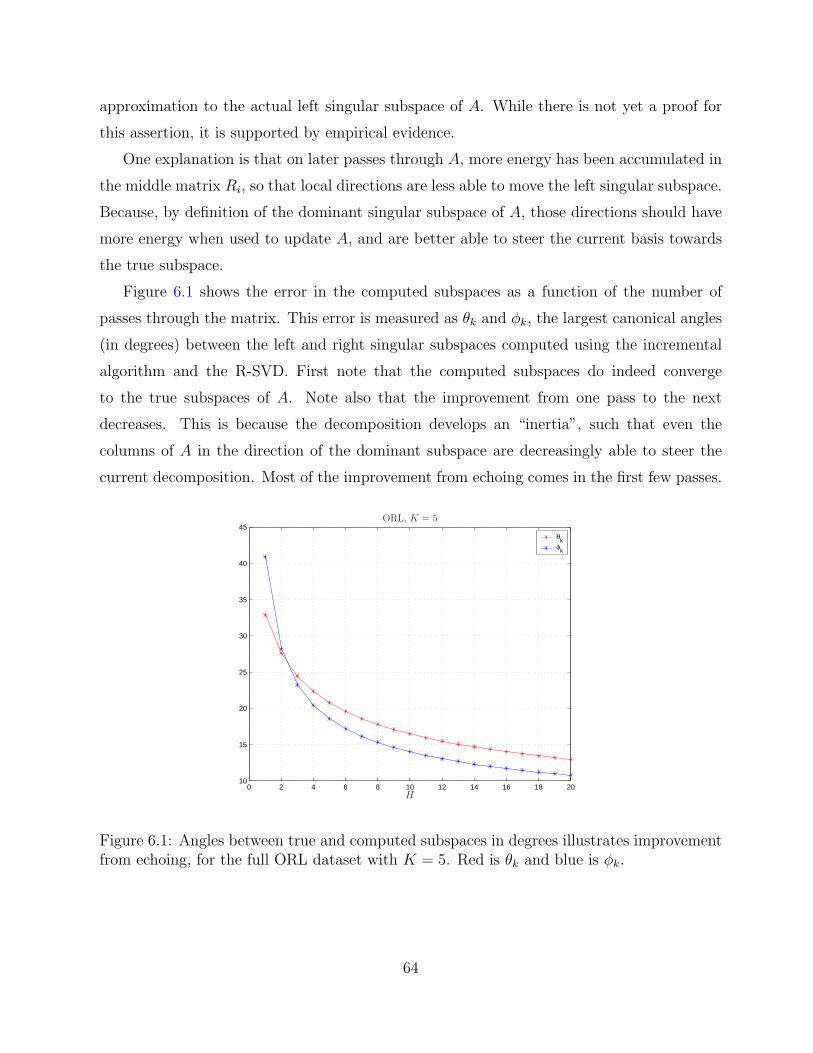
approximation to the actual left singular subspace of A. While there is not yet a proof for

this assertion, it is supported by empirical evidence.

One explanation is that on later passes through A, more energy has been accumulated in

the middle matrix Ri, so that local directions are less able to move the left singular subspace.

Because, by definition of the dominant singular subspace of A, those directions should have

more energy when used to update A, and are better able to steer the current basis towards

the true subspace.

Figure 6.1 shows the error in the computed subspaces as a function of the number of

passes through the matrix. This error is measured as θk and φk, the largest canonical angles

(in degrees) between the left and right singular subspaces computed using the incremental

algorithm and the R-SVD. First note that the computed subspaces do indeed converge

to the true subspaces of A. Note also that the improvement from one pass to the next

decreases. This is because the decomposition develops an “inertia”, such that even the

columns of A in the direction of the dominant subspace are decreasingly able to steer the

current decomposition. Most of the improvement from echoing comes in the first few passes.

0 2 4 6 8 10 12 14 16 18 2010

15

20

25

30

35

40

45θ

kφ

k

H

ORL, K = 5

Figure 6.1: Angles between true and computed subspaces in degrees illustrates improvementfrom echoing, for the full ORL dataset with K = 5. Red is θk and blue is φk.

Applying GenInc to B =[A A

]requires approximately twice as much work as running

65

Figure 6.1: Angles between true and computed subspaces in degrees illustrates improvementfrom echoing, for the full ORL dataset with K = 5. Red is θk and blue is φk.

64

Applying GenInc to B =[A A

]requires approximately twice as much work as running

one on A. The amount of post-processing necessary depends on the desired result:

• No post-processing is required to compute a basis for the dominant left singular

subspace;

• Producing an orthonormal basis for the dominant right singular subspaces requires a

QR factorization of V T2 = QvRv (cost: O(nk2));

• Producing dominant singular values of B requires computing the SVD of ΣRTv (cost:

O(k3)), in addition to the steps above;

• Producing the dominant left and right singular vectors of B requires matrix multipli-

cations (cost: 2mk2 and 2nk2, respectively), in addition to the steps above.

Echoing has been shown to produce a worthwhile increase in the result of the incremental

algorithm. Unlike the pivoting algorithm, echoing is easy to implement, requiring few changes

to the code. The only requirement is that the columns of A are available for processing

multiple times in a read-only fashion. Furthermore, this method requires no additional work

space, as long as the incremental algorithm does not start producing the right singular basis

until the appropriate step.

6.3 Partial Correction

The incremental algorithms described in this thesis partially produce a decomposition for

the matrix A of the form

A = UMV T =[U U⊥

] [Σ A1,2

0 A2,2

] [V V⊥

]T. (6.4)

The modifier “partial” is added because the incremental algorithms only produce the

matrices U , Σ, and V , and not their complements.

This decomposition is to be compared against the true singular value decomposition of

A, partitioned conformally,

A =[U1 U2

] [Σ1 00 Σ2

] [V1 V2

]T. (6.5)

The goal of the incremental algorithm is to compute approximate bases for the dominant

subspaces U1 and V1. These approximations are the U and V shown in Equation (6.4).

65

The matrix M =

[Σ A1,2

0 A2,2

]contains all of the information necessary to correct our

approximations, provided the SVD of M and the complements U⊥ and V⊥ were available.

Assuming that U⊥ and V⊥ were available, the update would follow trivially. First,

compute the matrix M = UT AV and the SVD M = UMΣMV TM . Then use this SVD to

update the computed matrices as follows,

Unew = UUM

Σnew = ΣM

Vnew = V VM

Note that this method computes exactly the singular value decomposition of A, com-

pletely correcting the bases U and V and the singular values Σ. This approach is very

similar to the R-SVD method. This similarity includes the high cost, unfortunately. Without

even discussing how U⊥ and V⊥ were obtained, this correction requires 2mn2 + O(n3) for

the production of M , another O(n3) for the SVD of M , and a final 2mnk + 2n2k for the

production of the first k columns of U1 and V1. A user willing and able to invest the resources

(time and storage) required for this operation could obtain the dominant SVD of A from the

R-SVD.

Other methods exist for finding the dominant singular subspaces of M . In [16][17],

Stewart and Mathias propose an iterative technique for driving a block triangular matrix

to block diagonal. Applying this method to M would iteratively improve the computed

subspaces. However, this method still requires that the matrix M is available, in addition

to the basis complements U⊥ and V ⊥.

These techniques can be approximated, requiring much less work and space. Assuming

the availability of some matrix U which approximates the dominant left singular subspace

of A. Given some basis Up, of rank p and orthogonal to U , compute the matrix M ,

B.=

[U Up

]M = BT A.

66

Compute the SVD of M = UMΣMV TM

and use these matrices to update the decomposition:

Unew = BUM

Σnew = ΣM

Vnew = VM .

Because UMΣMV TM

= BT A, then BUMΣMV TM

= BBT A. Then the SVD computed by this

partial correction step is the exact SVD of the projection of A onto the space R(B). This

result has multiple consequences.

The first consequence is that, given B whose range contains the true dominant subspace

of A, this correction step will produce the true dominant singular subspace and singular

values of A. This is easily proven and results from the fact that the dominant SVD of A is

invariant under projection down to the dominant singular subspace of A.

The second consequence is that only one correction step is worthwhile using a specific

basis B. This is because the result of a correction is the dominant SVD of A projected to

R(B); if B is kept the same, then the result will not change.

An implementation for this correction requires a basis U for which improvement is

desired, along with some basis Up to expand the space. It has already been stated that

if R(U1) ⊆ R(U) ∪ R(Up), then the correction will yield the exact dominant SVD of A.

Having computed U by applying GenInc to A, the motivating desire is that it approximates

the dominant SVD of A fairly well. However, without some other knowledge about the

dominant left singular subspace of A, there is no way to select Up to complete the space

R(U1).

The issue remains on how to select Up. A random basis, chosen orthogonal to U , will

not help to complete R(U) (with respect to R(U1)). The reason is that, because m � n,

a randomly chosen basis will likely not contain any information in R(A), least of all in

R(U1) ⊂ R(A).

One proposal for Up is to use the discarded vectors Qf from the last step of the

incremental algorithm. Another possibility is to take the first p columns of A and use

them to construct Up, by orthogonalizing them against U . This first proposal is attractive

because it requires only an extra matrix multiply to produce on the last incremental step

(cost: 2m(k + p)p), while the second proposal requires a Gram-Schmidt orthogonalization

of A(1:p) (cost: 4m(k + p)p). However, for the first method, the value of p is determined by

67

the number of vectors discarded on the last step, while p is determined by the user for the

second method. The partial correction method described here works increasingly well for

larger values of p, so that one may not wish to be limited in the choice of p.

Once Up is determined, the partial correction step proceeds as described above. The cost

is outlined here:

• 2mn(k + p) for the production of M = BT A, requiring (k + p)n memory to store the

result,

• 4n(k + p)2 +2nk(k + p)+O(k3 + p3) for the dominant SVD of M , via the R-SVD, and

• 2mk(k + p) to produce the first k columns of Unew, requiring mk memory for work

space.

Note that all of these terms are linear in both m and n, the dimensions of A. The only

usage of A is in the multiplication BT A, which can be easily streamed. If p = n, the total

cost is 4mnk + 4mk2 + 20nk2 + O(k3). Considering m � n and n � k, this term can be

simplified to 4mnk.

Table 6.2 shows the improvement using the Partial Correction method, compared against

Echoing. GenInc was applied to the COIL20-720 dataset, with K = 5. Running the data

again with twice Echoing, the errors in the subspaces are reduced, at a cost of double that

for the GenInc. However, for a partial correction with p = k on the basis produced by the

basic GenInc, the quality of the bases exceeds that of those produced using Echoing, at a

much lower cost. Furthermore, when p is allowed to increase so that the cost of the Partial

Correction approaches that of the Echoing, the quality of the produced bases increases even

further. The partial complement Up was computed in these experiments using two steps of

classical Gram-Schmidt reorthogonalization on the first p columns of A.

The process described above computes the exact SVD of the projection of A onto the

range of B. However, if the expense of the SVD of M in this technique is still too high,

there are approximation techniques to reduce the computational and memory requirements.

One possibility is to approximate the SVD of M of via a low-rank incremental, such as the

GenInc. Another possibility is to use the method of Stewart and Mathias [16][17] to improve

the estimated subspaces. Both of these techniques will approximately compute the SVD of

the projection of A onto the range of B.

68

Table 6.2: Partial Completion compared against a one-pass incremental method, with andwithout Echoing, for the C20-720 data with K = 5.

Cost tan(θk) tan(φk)GenInc 10mnk 3.234199 4.242013Echoing (h = 2) 20mnk 2.594525 2.740707Partial Correction (p = k) 14mnk 2.285459 1.812507Partial Correction (p = 2k) 16mnk 2.018349 1.589710Partial Correction (p = 4k) 20mnk 1.851909 1.448108

6.4 Summary

This chapter proposes three methods for improving the quality of the bases computed by

allowing extra read-only incremental passes through an incremental algorithm. The first

method, Pivoting, outlines a general strategy for improving the quality of the bases by

processing the columns of A in a different order. A simple heuristic for determining this

order is proposed and improvements are demonstrated for a random matrix. A second

method is described, Echoing, that processes the matrix A multiple times. This simple idea

is demonstrated to yield improvements in both the computed dominant singular vectors and

values, most notably in the right singular subspace. Finally, a third method is proposed,

Partial Correction, which uses an approximation of a method known to compute the

exact SVD. This technique is shown to be capable of better results than Echoing, with

a significantly lower cost. Further approximations to Partial Correction are suggested to

reduce the cost of the algorithm.

69

CHAPTER 7

CONCLUSION

Incremental algorithms for tracking the dominant singular subspaces of a matrix have been

studied numerous times before. Many authors have described the same heuristic for tracking

these subspaces, but they have each produced different methods with differing results and

requirements. This thesis presents a generic algorithm for incrementally computing the

dominant singular subspaces of a large matrix. This framework unifies the works of the

previous authors, clarifying the differences between the previous methods in a way that

illustrated the varying results. This common framework also allowed a transference of

analyses to be made, from method to method. Furthermore, this framework demonstrates

exactly what is necessary to compute the subspaces, and by doing so, is able to produce a

more efficient method than those previously described. This efficiency is shown to be present

across a greater range of operating parameters, and is illustrated empirically with application

data. Recommendations are made that suggest which method should be used under which

operating conditions, whether they are parametric (such as block size or data dimension) or

architectural (such as primitive efficiency).

This work illustrates the benefits of a block algorithm over a scalar one. The benefits

are computational, in terms of decreased runtime. Block algorithms, despite having a larger

operation count, outperform scalar algorithms when using level-3 primitives which exploit

a modern memory hierarchy. The benefits are numerical, with a larger block size yielding

potential improvement in the computed results. The effect of increasing block size on existing

error analyses is also discussed, with numerous corrections and additions made to the work

of the previous authors. In particular, the approximate bounds of Chahlaoui et al. are shown

to be more reliable as the block size is increased.

Finally, novel methods are proposed to improve the quality of the computed factorization

70

and subspaces, when allowed a second pass through the matrix. A general “pivoting”

framework is described, and a heuristic is proposed to implement it. This simple method is

empirically illustrated to give the intended improvements in the computed results. Echoing,

a straightforward method for passing multiple times through the data matrix, is heuristically

motivated, and empirically demonstrated to be effective in producing a better result. Lastly,

Partial Correction describes a method for correcting the dominant subspaces, using a low-

rank approximation of a method known to produce the exact singular value decomposition.

7.1 Future Work

The generic incremental algorithm proposed by this thesis is still a very heuristic one, and it

is difficult to say anything in a rigorous fashion without making some assumptions about the

nature of the matrix A and its singular value decomposition. Many areas of future work exist

in this thread. As the matrices Gu and Gv describe whether the current space is evolving

during each update, these matrices may be analyzed for clues as to the convergence of the

tracked subspaces. Also, the second-pass echoing method described in Chapter 6 should be

studied in more detail. Possibilities for improvement include a method for selective echoing

of input data, based perhaps on some characteristic of the previously associated update step;

or an analysis of convergence of this method.

71

APPENDIX A

Proof of the Complete Decomposition

It is stated in [11] that, at each step i of the incremental algorithm, there exists an orthogonal

matrix Vi such that

A(1:i)Vi = A(1:i)

[Wi W⊥

i

]=

[QiRi q1ρ1 . . . qiρi

].

and such that Vi embeds Wi as shown above.

This result is used to derive error bounds on the factorization produced by the incremental

algorithm. However, this result is never proven in the discussion of the scalar algorithm. This

appendix shows that the above holds not only for the li = 1 scalar case, for the block case

in general.

First, note that the first step of the algorithm updates the factorization A(1:s0) = Q0R0

to

A(1:s1) = QRGTv

=[Q1 Q1

] [R1 0

0 R1

] [W1 W1

]T.

Then choosing V1 = Gv =[W1 W1

], it follows that

A(1:s1)V1 =[Q1 Q1

] [R1 0

0 R1

]=

[Q1R1 Q1R1

],

showing the desired result for our base case of i = 1.

Now, assume for the purpose of induction that this result holds after step i. Then there

exists a matrix Vi such that

A(1:si)Vi = A(1:si)

[Wi W⊥

i

]=

[QiRi Q1R1 . . . QiRi

].

72

The i + 1st step of the algorithm updates the current factorization, QiRiWTi with the

columns A+ = A(si+1:si+1), like so:

[QiRiW

Ti A+

]=

[Qi Q⊥

]GuG

Tu

[Ri C0 R⊥

]GvG

Tv

[Wi 00 I

]T

=[Qi+1 Qi+1

] [Ri+1 0

0 Ri+1

] [Wi+1 Wi+1

]T.

Consider the matrix

Vi+1 =

[Vi 00 Il

]P

[Gv 00 Isi−k

]P T ,

where

P =

Ik 0 00 0 Isi

0 Il 0

.

Then

A(1:si+1)Vi+1 =[A(1:si) A+

] [Vi 00 Il

]P

[Gv 00 Isi−k

]P T

=[QiRi Q1R1 . . . QiRi A+

]P

[Gv 00 Isi−k

]P T

=[QiRi A+ Q1R1 . . . QiRi

] [Gv 00 Isi−k

]P T

=[Qi+1Ri+1 Qi+1Ri+1 Q1R1 . . . QiRi

]P T

=[Qi+1Ri+1 Q1R1 . . . Qi+1Ri+1

],

as required.

Vi+1 is orthogonal, obviously satisfying V Ti+1Vi+1 = Ik. Furthermore, it is easily shown

that Vi+1 embeds Wi+1 as desired:

Vi+1 =

[Vi 00 Il

]P

[Gv 00 Isi−k

]P T

=

[Wi W⊥

i 00 0 I

]P

[Gv 00 Isi−k

]P T

=

[Wi 0 W⊥

i

0 I 0

] [Gv 00 Isi−k

]P T

=

[Wi+1 Wi+1

W⊥i

0

]P T

=

[Wi+1

W⊥i

0Wi+1

]=

[Wi+1 W⊥

i+1

].

73

Each Vi then has the correct form and affect on A(1:si), and consists of the transformation

Gv from each step of the algorithm along with specific permutations, as characterized in [11].

Note also that each W⊥i has a block upper trapezoidal structure:

W⊥i =

[W⊥

i−1

0Wi

],

with diagonal blocks of order di. This result facilitates the error analyses in this thesis.

It should also be noted that this proof made no assumptions about the structure of Ri

at each step, i.e. it may be diagonal (as in the SKL), triangular (as in the Recursive SVD),

or unstructured (as in the generic incremental method presented in this paper.)

Then after f steps of the incremental algorithm, where all columns of A have been

processed, there exists by the result above the decomposition

AVf = A[Wf W⊥

f

]=

[QfRf Q1R1 . . . Qf Rf

].

The SVD of Rf = UΣV T yields the factorization

AV = A[Wf V W⊥

f

]=

[Qf U Q⊥

f

] [Σ A1,2

0 A2,2

]= U

[Σ A1,2

0 A2,2

],

where Q⊥f is orthogonal to Qf . Define A2 as follows:

A2.=

[A1,2

A2,2

]with µ

.= ‖A2‖2. Note that this gives an additive decomposition for A:

A = U

[Σ A1,2

0 A2,2

]V T

=[Qf U Q⊥

f

] [Σ A1,2

0 A2,2

] [Wf V W⊥

f

]T

= QfRfWTf + UA2W

⊥f

T.

Then the norm of the residual error in the approximation A ≈ QfRfWTf is

‖A−QfRfWTf ‖2 = ‖QfRfW

Tf + UA2W

⊥f

T −QfRfWTf ‖2

= ‖UA2W⊥f

T‖2 = µ.

74

APPENDIX B

On WY-Representations of Structured Householder

Factorizations

Bischof and Van Loan describe in [13] how the product of d Householder reflectors can be

represented in a block form, H1H2 · · ·Hd = I+WY T . When computing the QR factorization

of a structured matrix, the reflectors may in turn have some structure, and this can show

up in W and Y .

The method in 3.3.4.2 describes the transformation of the k + d× d matrix U2STu , having

the lower trapezoidal form

U2STu =

[LB

],

This matrix is transformed by the matrix Gu, so that

GTu (U2S

Tu ) =

[0Id

].

This is done by computing the QL factorization of the matrix U2STu . It is also equivalent

to computing the QR factorization of the matrix U.= E1(U2S

Tu )E2, where E1 and E2 are

permutation matrices that reverse the order of the rows and columns of U2STu , respectively.

This work considers the latter case, the QR factorization of the permuted matrix, U .

First, note some properties of U . It is orthogonal, so the QR factorization produces a

matrix which is both orthogonal and upper triangular, and therefore a diagonal matrix with

unit-elements. Also note the structure of U :

U =

[BU

].

Then the first column of the the matrix only has k+1 non-zeroes. Then the first reflector

matrix, H1, needs only be of order k + 1 and modifies only the first k + 1 rows of the matrix

75

U . Furthermore, because U has orthonormal columns, then the first column is transformed

to the elementary basis vector e1 and the rest of the first row consists of zeroes. This is

illustrated by the following:

Hd · · ·H2H1U = Hd · · ·H2

[H1 00 Id−1

] [b0 B0

0 U0

]= Hd · · ·H2

[e1 H1B0

0 U0

]

= Hd · · ·H3

1 0 0

0 H2 00 0 Id−2

1 0 00 b1 B1

0 0 U1

= Hd · · ·H3

I2 0 00 b3 B3

0 0 U3

= · · ·

=

[Id

0

].

This process continues until U has been reduced to an upper triangular matrix, whose

triangular part is the identity (up to sign). This is effected by a sequence of Householder

reflectors, each of order k + 1. Each of these reflectors has the form Hi = Ik+d + βiuiuTi .

But the reduced order of these transformations reveals an additional structure, also shown

above:

Hi = Ik+d + βiuiuTi =

Ii−1 0 0

0 Hi 00 0 Id−i

ui =

0i−1

1ui

0d−i

Hi = Ik+1 + βiuiu

Ti .

It is assumed that the Householder vector defining each reflector has 1 as its first non-

zero. This is typical (see [1], page 210), but not necessary. If this is not the case, it has only

minor consequences that are discussed later.

Bischof and Van Loan describe the how W and Y may be built from βi the individual

reflectors. The resulting factorization, I + WY T , has the same numerical properties as

the individual Householder reflectors, but has the benefit of using level 3 primitives in

76

its application. Furthermore, it is later shown that when W and Y are constructed from

reflectors structured like those Hi above, they have the structure:

W =

[BU

]and Y =

LBU

, (B.1)

where U represents an upper triangular matrix, B represents an unstructured matrix, and

L represents a unit-diagonal, lower triangular matrix.

The structure of W and Y follows simply from their construction. Let W(1) and Y(1) be

defined as follows:

W(1) = β1u1 =

β1

β1u1

0d−1

Y(1) = u1 =

1u1

0d−1

.

Then trivially, I + W(1)YT(1) = I + βu1u

T1 = H1, and W and Y have structure agreeing

with that of (B.1).

Now assume for the purpose of induction that W(i) and Y(i) have the structure, dictated

in (B.1):

W(i) =

BU

0d−i

and Y(i) =

LBU

0d−i

,

and that I +W(i)YT(i) = H1 · · ·Hi, so that W(i) and Y(i) have the desired effect of the product

of the first i Householder reflectors.

Bischof and Van Loan describe the update of W(i) and Y(i) as follows:

W(i+1) =[W(i) (I + W(i)Y

T(i))βi+1ui+1

]Y(i+1) =

[Y(i) ui+1

].

Then the effect of I + W(i+1)YT(i+1) is trivially shown as the accumulation of the

Householder reflectors up to and including Hi+1:

I + W(i+1)YT(i+1) = I +

[W(i) (I + W(i)Y

T(i))βi+1ui+1

] [Y(i) ui+1

]T

= I + W(i)YT(i) + (I + W(i)Y

T(i))βi+1ui+1u

Ti+1

= (I + W(i)YT(i))(I + βi+1ui+1u

Ti+1)

= H1 · · ·Hi+1.

77

As for the structure of W(i+1) and Y(i+1), this is easily demonstrated. First, consider

Y(i+1):

Y(i+1) =[Y(i) ui+1

]

=

L 0i

BU0

1ui+1

0d−i−1 0d−i−1

=

L′

B′

0d−(i+1)

.

Consisting of only the ui matrix from each step, stacked back to back, the structure of

Y is a trivial result of the structure in ui.

Next, consider W(i+1). The last column of W(i+1) is the product (I + W(i)YT(i))βi+1ui+1.

Its structure is shown to be:

(I + W(i)YT(i))βi+1ui+1 = βi(ui+1 + W(i)z)

= βi(

0i

1u(i+1)

0d−i−1

+

BzUz0

0d−i−1

)

=

[w1

0d−i−1

]+

[w2

0d−i−1

]=

[w

0d−i−1

].

Then W(i+1) has the structure

W(i+1) =

BU0

w

0d−i−1 0d−i−1

=

B′

U ′

0d−(i+1)

.

After the accumulation of d reflectors, then it follows that W and Y have the structure

W =

[Bw

Uw

]and Y =

Ly

By

Uy

,

where B are unstructured matrices, U are upper triangular matrices, and Ly is a unit-

diagonal, lower-triangular matrix. Note that in the case that the leading non-zero of each

78

Householder vector ui is not 1, then Ly does not have unit diagonal elements. This has little

bearing on the algorithm, with respect to computation or storage.

It has been shown then the form and construction method of a structured transformation

that sends U to

[I0

]. This method can be modified to operate on the matrix U2S

Tu , yielding

the same transformation. Note that[0k

Id

]= E1

[Id

0k

]E2

= E1(Hd · · ·H1)UE2

= E1(I + Y W T )UE2

= E1(I + Y W T )E1E1UE2

= (I + E1Y E2E2WT E1)(U2S

Tu )

= GTu (U2S

Tu ),

where Gu = I + (E1WE2)(E1Y E2)T , and has structure

Gu = I + (E1WE2)(E1Y E2)T

= I +

(E1

[Bw

Uw

]E2

) E1

Ly

By

Uy

E2

T

= I +

[L′

w

B′w

] [U ′

y B′y L′

y

].

79

APPENDIX C

Testing Specifications

The timings presented in Section 4.1 were performed on a Sun Ultra-80, with 1 gigabyte

of memory and dual 450MHz Ultra-II processors. The compiler used was the Fortran 95

compiler from the Sun Workshop 6, Update 2. The version of ATLAS was version 3.5.0.

The version of the Netlib BLAS and LAPACK libraries was version 3.0 with the May, 2000

update.

The compiler options used to compile both the incremental libraries and the testing

executable were:

FLAGS=-fast -ftrap=%none -fsimple=0 -fns=no

F90=f95 -dalign -w2 ${FLAGS}

Timing was performed in the executable, using the gethrtime subroutine.

80

REFERENCES

[1] G. Golub and C. Van Loan. Matrix Computations. The Johns Hopkins University Press,Baltimore, third edition, 1996. 1, 4, 76

[2] G. W. Stewart. Matrix Algorithms, Volume I: Basic Decompositions. Society forIndustrial and Applied Mathematics, Philadelphia, 1998. 1, 21

[3] L. Sirovich. Empirical eigenfunctions and low dimensional systems. In L. Sirovich,editor, New Perspectives in Turbulence, pages 139–163. Springer, New York, 1991. 3

[4] J. Lumley. The structure of inhomogeneous turbulent flows. In A. Yaglom andV. Tatarsky, editors, Atmospheric Turbulence and Radio Wave Propagation, page 166.Nauka, Moscow, 1967. 3

[5] L. Sirovich. Turbulence and the dynamics of coherent structures. Part I: Coherentstructures. Quarterly of Applied Mathematics, 45(3):561–571, October 1987. 3

[6] M. Gu and S. C. Eisenstat. A stable and fast algorithm for updating the singular valuedecomposition. Technical Report YALEU/DCS/RR-966, Yale University, New Haven,CT, 1993. 7, 17

[7] S. Chandrasekaran, B. S. Manjunath, Y. F. Wang, J. Winkeler, and H. Zhang. Aneigenspace update algorithm for image analysis. Graphical models and image processing:GMIP, 59(5):321–332, 1997. 8, 44

[8] B. S. Manjunath, S. Chandrasekaran, and Y. F. Wang. An eigenspace update algorithmfor image analysis. In IEEE Symposium on Computer Vision, page 10B ObjectRecognition III, 1995. 8, 43, 48

[9] A. Levy and M. Lindenbaum. Sequential Karhunen-Loeve basis extraction and itsapplication to images. IEEE Transactions on image processing, 9(8):1371–1374, August2000. 9, 45, 46, 47

[10] M. Brand. Incremental singular value decomposition of uncertain data with missingvalues. In Proceedings of the 2002 European Conference on Computer Vision, 2002. 10

[11] Y. Chahlaoui, K. Gallivan, and P. Van Dooren. Recursive calculation of dominantsingular subspaces. SIAM J. Matrix Anal. Appl., 25(2):445–463, 2003. 10, 11, 72, 74

81

[12] Y. Chahlaoui, K. Gallivan, and P. Van Dooren. An incremental method for computingdominant singular spaces. In Computational Information Retrieval, pages 53–62. SIAM,2001. 16, 19, 21, 42, 48, 49, 50, 51, 54, 57

[13] C. Bischof and C. Van Loan. The WY representation for products of Householdermatrices. SIAM J. Sci. Stat. Comput., 8:s2–s13, 1987. 25, 75

[14] G. W. Stewart and J.-G. Sun. Matrix Perturbation Theory. Academic Press, San Diego,1990. 49

[15] S. Geman. A limit theorem for the norm of random matrices. Annals of Probability,8(2):252–261, April 1980. 51

[16] G. W. Stewart. On an algorithm for refining a rank-revealing URV decomposition anda perturbation theorem for singular values. Technical Report CS-TR 2626, Departmentof Computer Science, University of Maryland, 1991. Revised version appeared as [17].66, 68

[17] R. Mathias and G. W. Stewart. A block QR algorithm and the singular valuedecomposition. Linear Algebra and Its Applications, 182:91–100, 1993. 66, 68, 82

82

BIOGRAPHICAL SKETCH

Christopher G. Baker

Christopher Grover Baker was born on September 5, 1979, in Marianna, Florida, to Frank

and Lynn Baker. In the spring of 2002, he completed his Bachelors degree in Computer

Science and Pure Mathematics at The Florida State University. Under the advisement of

Prof. Kyle Gallivan, he obtained his Masters degree in summer of 2004, also from the

Department of Computer Science at FSU. He enrolled in the doctoral program at FSU in

the fall of 2004. Legend holds that he still remains there.

Chris’s research interests include numerical linear algebra, computer graphics, scientific

visualization, numerical optimization, and high performance computing.

Chris lives in Tallahassee, FL, with his wife Kelly Baker, a doctoral student in the

Department of Religious Studies at FSU. They have two dogs and one cat.

Chris is a member of ACM, IEEE, and SIAM.

83