A biomimetic basis for the perception of

natural sounds

H. Ammari and B. Davies

Research Report No. 2020-32May 2020

Seminar für Angewandte MathematikEidgenössische Technische Hochschule

CH-8092 ZürichSwitzerland

____________________________________________________________________________________________________

A biomimetic basis for the perception of natural sounds

Habib Ammari∗ Bryn Davies∗

Abstract

Arrays of subwavelength resonators can mimic the biomechanical properties of the cochlea, at

the same scale. We derive, from first principles, a modal time-domain expansion for the scattered

pressure field due to such a structure and propose that these modes should form the basis of a signal

processing architecture. We investigate the properties of such an approach and show that higher-order

gammatone filters appear by cascading. Further, we propose an approach for extracting meaningful

global properties from the coefficients, tailored to the statistical properties of so-called natural sounds.

Mathematics Subject Classification (MSC2010): 35C20, 94A12, 35J05, 31B10

Keywords: subwavelength resonance, metamaterials, auditory processing, gammatone filters,convolutional networks

1 Introduction

1.1 Biomimetic signal processing

Humans are exceptionally good at recognising different sound sources in their environment and therehave been many attempts at designing artificial approaches that can replicate this feat. The humanauditory system first amplifies and filters sounds biomechanically in the peripheral auditory system beforeprocessing the transduced neural signals in the central auditory signal. With a view to trying to mimicthis world-beating system, we consider using an artificial routine with a similar two-step architecture:physical filtering followed by additional processing stages.

There has been much attention paid to designing biomimetic structures that replicate the biomechan-ical properties of the cochlea [1–7]. At the heart of any such structure are graded material parameters,so as to replicate the spatial frequency separation of the cochlea. In particular, a size-graded array ofsubwavelength resonators can be designed to have similar dimensions to the cochlea and respond to anappropriate range of audible frequencies [1]. An acoustic subwavelength resonator is a cavity with ma-terial parameters that are greatly different from the background medium [3]. Bubbly structures of thiskind can be constructed, for example, by injecting air bubbles into silicone-based polymers [8, 9].

A graded array of resonators effectively behaves as a distributed system of band-pass filters [10]. Thechoice of kernel filter for auditory processing has been widely explored. Popular options include windowedFourier modes [11,12], wavelets [13–17] and learned basis functions [18]. In particular, gammatone filters(Fourier modes windowed by gamma distributions) have been shown to approximate auditory filterswell and, thanks also to their relative simplicity, are used widely in modelling auditory function as aresult [10, 19–21]. We will prove that, at leading order, an array of N subwavelength resonators behavesas an array of N gammatone filters.

The human auditory system is known to be adapted to the structure of the most important inputsand exhibits greatly enhanced neural responses to natural and behaviourally significant sounds such asanimal and human vocalisations and environmental sounds [22]. It has been observed that such sounds,often known collectively as natural sounds, display certain statistical properties [22–25]. By design, mostmusic also falls into this class; music satisfying these properties sounds “much more pleasing” [23]. Thus,it is clear that the human auditory system is able to account for global properties of a sound and thata biomimetic processing architecture needs to replicate this. Many attempts have been made to extractthese. We propose using the parameters of the observed statistical distributions as meaningful andtractable examples of global properties to be used in artificial representations of auditory signals.

∗Department of Mathematics, ETH Zurich, Ramistrasse 101, CH-8092 Zurich, Switzerland.B habib.ammari@math.ethz.chB bryn.davies@sam.math.ethz.ch

1

≪ wavelength

ρ, κρb, κb

Figure 1: A graded array of subwavelength resonators.

1.2 Main Contributions

In Section 3 we derive results that describe the resonant properties of a system of N resonators in threedimensions and prove a modal decomposition in the time domain. This formula takes the form of Nspatial eigenmodes with first-order gammatone coefficients. Further to this, we show in Section 4 that acascade of these filters equates to filtering with higher-order gammatones and that extracting informationfrom temporal averages is stable to deformations. Finally, in Section 5.1 we focus our attention on theclass of natural sounds, which we define as sounds satisfying certain (widely observed) statistical andspectral properties. Using these properties, we propose a parametric coding approach that extracts theglobal properties of a sound.

2 Boundary integral operators

2.1 Problem setting

We are interested in studying wave propagation in a homogeneous background medium with N ∈ N

disjoint bounded inclusions, which we will label as D1, D2, . . . , DN ⊂ R3. We will assume that the

boundaries are all Lipschitz continuous and will write D = D1 ∪ · · · ∪ DN . In order to replicate thespatial frequency separation of the cochlea, we are interested in the case where the array has a sizegradient, meaning each resonator is slightly larger than the previous, as depicted in Figure 1.

We will denote the density and bulk modulus of the material within the bounded regions D by ρband κb, respectively. The corresponding parameters for the background medium are ρ and κ. The wavespeeds in D and R

3 \D are given by

vb =

√

κbρb, v =

√

κ

ρ.

We also define the dimensionless contrast parameter

δ =ρbρ.

We will assume that δ ≪ 1, meanwhile vb = O(1), v = O(1) and vb/v = O(1).

2.2 Boundary integral operators

The Helmholtz single layer potential associated to the domain D and wavenumber k ∈ C is defined, forsome density function ϕ ∈ L2(∂D), as

SkD[ϕ](x) :=

∫

∂D

G(x− y, k)ϕ(k) dσ(y), x ∈ R3,

where G is the Helmholtz Green’s function, given by

G(x, k) := − 1

4π|x|eik|x|.

The Neumann-Poincare operator associated to D and k ∈ C is defined as

Kk,∗D [ϕ](x) :=

∫

∂D

∂G(x− y, k)

∂ν(x)ϕ(y) dσ(y), x ∈ ∂D,

2

where ∂/∂ν denotes the outward normal derivative on ∂D. These two integral operators are related bythe conditions

∂

∂νSkD[ϕ]

∣

∣

±(x) =

(

±1

2I +Kk,∗

D

)

[ϕ](x), x ∈ ∂D, (2.1)

where the subscripts + and − denote evaluation from outside and inside the boundary ∂D, respectively,and I is the identity operator on L2(∂D).

2.3 Asymptotic properties

The single layer potential and the Neumann–Poincare operator both have helpful asymptotic expansionsas k → 0 (see e.g. [26]). In particular, we have that

SkD[ϕ] = SD[ϕ] + kSD,1[ϕ] +O(k2), (2.2)

where SD := S0D (i.e. the Laplace single layer potential) and

SD,1[ϕ](x) :=1

4πi

∫

∂D

ϕ(y) dσ(y).

One crucial property to note is that SD is invertible. Similarly,

Kk,∗D [ϕ] = K∗

D[ϕ] + kKD,1[ϕ] + k2KD,2[ϕ] + k3KD,3[ϕ] +O(k4), (2.3)

where K∗D := K0,∗

D , KD,1 = 0,

KD,2[ϕ](x) :=1

8π

∫

∂D

(x− y) · ν(x)|x− y| ϕ(y) dσ(y) and KD,3[ϕ](x) :=

i

12π

∫

∂D

(x− y) · ν(x)ϕ(y) dσ(y).

Several of the operators in the expansion (2.3) can be simplified when integrated over all or part ofthe boundary ∂D. As proved in e.g. [27, Lemma 2.1], it holds that for any ϕ ∈ L2(∂D) and i = 1, . . . , N ,

∫

∂Di

(

−1

2I +K∗

D

)

[ϕ] dσ = 0,

∫

∂Di

(

1

2I +K∗

D

)

[ϕ] dσ =

∫

∂Di

ϕ dσ,

∫

∂Di

KD,2[ϕ] dσ = −∫

Di

SD[ϕ] dx and

∫

∂Di

KD,3[ϕ] dσ =i|Di|4π

∫

∂D

ϕ dσ.

(2.4)

3 Subwavelength scattering decompositions

3.1 Scattering of pure tones

Suppose, first, that the incoming signal is a plane wave parallel to the x1-axis with angular frequency ω,given by A cos(kx1 − ωt) where k = ω/v. Then, the scattered pressure field is given by Re(u(x, ω)e−iωt)where u satisfies the Helmholtz equation

{

(

∆+ k2)

u = 0 in R3 \D,

(

∆+ k2b)

u = 0 in D,(3.1)

where k = ω/v and kb = ω/vb, along with the transmission conditions

{

u+ − u− = 0 on ∂D,1ρ

∂u∂νx

∣

∣

+− 1

ρb

∂u∂νx

∣

∣

−= 0 on ∂D,

(3.2)

and the Sommerfeld radiation condition in the far field, which ensures that energy radiates outwards [26],given by

(

∂

∂|x| − ik

)

(u− uin) = o(|x|−1) as |x| → ∞, (3.3)

where, in this case, uin(x, ω) = Aeikx1 .

3

Definition 3.1 (Resonant frequency). We define a resonant frequency to be ω = ω(δ) such that thereexists a non-trivial solution to (3.1) which satisfies (3.2) and (3.3) when uin = 0.

Definition 3.2 (Subwavelength resonant frequency). We define a subwavelength resonant frequency tobe a resonant frequency ω that depends continuously on δ and is such that ω(δ) → 0 as δ → 0.

Lemma 3.3. A system of N subwavelength resonators exhibits N subwavelength resonant frequencieswith positive real parts, up to multiplicity.

Proof. This was proved in [3] and follows from the theory of Gohberg and Sigal [26, 28].

3.1.1 Capacitance matrix analysis

Our approach to solving the resonance problem is to study the (weighted) capacitance matrix, whichoffers a rigorous discrete approximation to the differential problem. We will see that the eigenstates ofthis N ×N -matrix characterise, at leading order in δ, the resonant modes of the system.

In order to introduce the notion of capacitance, we define the functions ψj , for j = 1, . . . , N , as

ψj := S−1D [χ∂Dj

],

where χA : R3 → {0, 1} is used to denote the characteristic function of a set A ⊂ R3. The capacitance

coefficients Cij , for i, j = 1, . . . , N , are then defined as

Cij := −∫

∂Di

ψj dσ.

We will need two objects involving the capacitance coefficients. Firstly, the weighted capacitance matrixCvol = (Cvol

ij ), given by

Cvolij :=

1

|Di|Cij ,

which has been weighted to account for the different sized resonators (see e.g. [27, 29, 30] for othervariants in slightly different settings). Secondly, we will want the capacitance sums contained in thematrix Csum = (Csum

ij ), given byCsum := JC,

where C = (Cij) is the matrix of capacitance coefficients and J is the N ×N matrix of ones (i.e. Jij = 1for all i, j = 1, . . . , N).

We define the functions Sωn , for n = 1 . . . , N , as

Sωn (x) :=

{

SkD[ψn](x), x ∈ R

3 \D,Skb

D [ψn](x), x ∈ D.

Lemma 3.4. The solution to the scattering problem (3.1) can be written, for x ∈ R3, as

u(x)−Aeikx1 =

N∑

n=1

qnSωn (x)− Sk

D

[

S−1D [Aeikx1 ]

]

(x) +O(ω),

for constants qn which satisfy, up to an error of order O(δω + ω3), the problem

(

ω2I − v2bδ Cvol)

q1...qN

= v2bδ

1|D1|

∫

∂D1S−1D [Aeikx1 ] dσ...

1|DN |

∫

∂DNS−1D [Aeikx1 ] dσ

.

Proof. The solutions can be represented as

u(x) =

{

Aeikx1 + SkD[ψ](x), x ∈ R

3 \D,Skb

D [φ](x), x ∈ D,(3.4)

4

for some surface potentials (φ, ψ) ∈ L2(∂D) × L2(∂D), which must be chosen so that u satisfies thetransmission conditions across ∂D. Using (2.1), we see that in order to satisfy the transmission conditionson ∂D, the densities φ and ψ must satisfy

Skb

D [φ](x)− SkD[ψ](x) = Aeikx1 , x ∈ ∂D,

(

−1

2I +Kkb,∗

D

)

[φ](x)− δ

(

1

2I +Kk,∗

D

)

[ψ](x) = δ∂

∂ν(Aeikx1), x ∈ ∂D.

Using the asymptotic expansions (2.2) and (2.3), we can see that

ψ = φ− S−1D [Aeikx1 ] +O(ω),

and, further, that

(

−1

2I +K∗

D +ω2

v2bKD,2 − δ

(

1

2I +K∗

D

))

[φ] = −δ(

1

2I +K∗

D

)

S−1D [Aeikx1 ] +O(δω + ω3). (3.5)

Then, integrating (3.5) over ∂Di, for 1 ≤ i ≤ N , and using the properties (2.4) gives us that

−ω2

∫

Di

SD[φ] dx− v2bδ

∫

∂Di

φ dσ = −v2bδ∫

∂Di

S−1D [Aeikx1 ] dσ +O(δω + ω3).

At leading order, (3.5) says that(

− 12I +K∗

D

)

[φ] = 0 so, in light of the fact that {ψ1, . . . , ψN} forms a

basis for ker(

− 12I +K∗

D

)

, the solution can be written as

φ =

N∑

n=1

qnψn +O(ω2 + δ), (3.6)

for constants q1, . . . , qN = O(1). Making this substitution we reach, up to an error of order O(δω + ω3),the problem

(

−ω2IN + v2bδCvol)

q1...qN

= −v2bδ

1|D1|

∫

∂D1S−1D [Aeikx1 ] dσ...

1|DN |

∫

∂DNS−1D [Aeikx1 ] dσ

. (3.7)

The result now follows by combining the above.

Theorem 3.5. As δ → 0, the subwavelength resonant frequencies satisfy the asymptotic formula

ω±n = ±

√

v2bλnδ − iτnδ +O(δ3/2),

for n = 1, . . . , N , where λn are the eigenvalues of the weighted capacitance matrix Cvol and τn are realnumbers that depend on D, v and vb.

Proof. If uin = 0, we find from Lemma 3.4 that there is a non-zero solution q1, . . . , qN to the eigenvalueproblem (3.4) when ω2/v2bδ is an eigenvalue of Cvol, at leading order.

To find the imaginary part, we adopt the ansatz

ω±n = ±

√

v2bλnδ − iτnδ +O(δ3/2). (3.8)

Using the expansions (2.2) and (2.3) with the representation (3.4) we have that

ψ = φ+kb − k

4πi

(

N∑

n=1

ψn

)

∫

∂D

φ dσ +O(ω2),

and, hence, that

(

−1

2I +K∗

D + k2bKD,2 + k3bKD,3 − δ

(

1

2I +K∗

D

))

[φ]− δ(kb − k)

4πi

(

N∑

n=1

ψn

)

∫

∂D

φ dσ = O(δω2 + ω4).

5

Figure 2: The resonant frequencies {ω+n, ω−

n: n = 1, . . . , N} in the complex plane, for an array of 22 subwavelength

resonators.

We then substitute the decomposition (3.6) and integrate over ∂Di, for i = 1, . . . , N , to find that(

−ω2

v2bI − ω3

v3b

i

4πCsum + δCvol + δω

(

1

vb− 1

v

)

i

4πCvolCsum

)

q = O(δω2 + ω4).

Then, using the ansatz (3.8) for ωn and setting q = vn (the eigenvector corresponding to λn) we reachthat

(

τnI −vbλn8π

Csum +

(

1− vbv

)

vb8πCvolCsum

)

vn = 0. (3.9)

Remark 3.6. The resonant frequencies will have negative imaginary parts, due to the loss of energy (e.g.to the far field), thus τn ≥ 0 for all n = 1, . . . , N .

Remark 3.7. Note that in some cases τn = 0 for some n, meaning the imaginary parts exhibit higher-order behaviour in δ. For example, the second (dipole) frequency for a pair of identical resonators isknown to be O(δ2) [27].

Remark 3.8. The numerical simulations presented in this work were all carried out on an array of 22cylindrical resonators. We approximate the problem by studying the two-dimensional cross section usingthe multipole expansion method, as in [1].

Remark 3.9. The array of 22 resonators that simulated in this work measures 35 mm, has materialparameters corresponding to air-filled resonators surrounded by water and has subwavelength resonantfrequencies within the range 500 Hz – 10 kHz. Thus, this structure has similar dimensions to the hu-man cochlea, is made from realistic materials and experiences subwavelength resonance in response tofrequencies that are audible to humans.

It is more illustrative to rephrase Lemma 3.4 in terms of basis functions that are associated with theresonant frequencies. Denote by vn = (v1,n, . . . , vN,n) the eigenvector of Cvol with eigenvalue λn. Then,we have a modal decomposition with coefficients that depend on the matrix V = (vi,j), provided thesystem is such that V is invertible.

Remark 3.10. The invertibility of V is a subtle issue and depends only on the geometry of the inclusionsD = D1∪· · ·∪DN . In the case that the resonators are all identical, V is invertible since Cvol is symmetric.If the size gradient is not too drastic, we expect V to also be invertible (this is supported by our numericalanalysis, which typically simulates an array of resonators where each is approximately 1.05 times the sizeof the previous).

Lemma 3.11. Suppose the resonator’s geometry is such that the matrix of eigenvectors V is invertible.Then if ω = O(

√δ) the solution to the scattering problem (3.1) can be written, for x ∈ R

3, as

u(x)−Aeikx1 =

N∑

n=1

anun(x)− SD

[

S−1D [Aeikx1 ]

]

(x) +O(ω),

for constants given by

an =−Aνn Re(ω+

n )2

(ω − ω+n )(ω − ω−

n ),

where νn =∑N

j=1[V−1]n,j, i.e. the sum of the nth row of V −1.

6

Proof. In light of (3.6), we define the functions

un(x) =

N∑

i=1

vi,n SD[ψi](x), (3.10)

for n = 1, . . . , N . Then, by diagonalising Cvol with the change of basis matrix V , we see that the solutionto the scattering problem (3.1) can be written as

u− uin =

N∑

n=1

anun − SD

[

S−1D [Aeikx1 ]

]

+O(ω),

for constants an given, at leading order, by

V

ω2 − v2bδλ1. . .

ω2 − v2bδλN

a1...aN

= v2bδ

1|D1|

∫

∂D1S−1D [Aeikx1 ] dσ...

1|DN |

∫

∂DNS−1D [Aeikx1 ] dσ

+O(ω3).

Now, ω2 − v2bδλn = (ω − ω+n )(ω − ω−

n ) +O(ω3) so we have that up to an error of order O(ω3)

a1...aN

= v2bδ

(ω − ω+1 )

−1(ω − ω−1 )

−1

. . .

(ω − ω+N )−1(ω − ω−

N )−1

V −1

1|D1|

∫

∂D1S−1D [Aeikx1 ] dσ...

1|DN |

∫

∂DNS−1D [Aeikx1 ] dσ

.

In order to simplify this further, we use the fact that eikx1 = 1 + ikx1 + · · · = 1 +O(ω) to see that

a1...aN

=

−Re(ω+1 )2

(ω−ω+1 )(ω−ω−

1 )

. . .−Re(ω+

N)2

(ω−ω+N)(ω−ω−

N)

V −1

A...A

+O(ω).

3.2 Modal decompositions of signals

Consider, now, the scattering of a more general signal, s : [0, T ] → R, whose frequency support is widerthan a single frequency and whose Fourier transform exists. Again, we assume that the radiation isincident parallel to the x1-axis. Consider the Fourier transform of the incoming pressure wave, given forω ∈ C, x ∈ R

3 by

uin(x, ω) =

∫ ∞

−∞

s(x1/v − t)eiωt dt

= eiωx1/v s(ω) = s(ω) +O(ω),

where s(ω) :=∫∞

−∞s(−u)eiωudu. The resulting pressure field satisfies the Helmholtz equation (3.1) along

with the conditions (3.2) and (3.3).Working in the frequency domain, the scattered acoustic pressure field u in response to the Fourier

transformed signal s can be decomposed in the spirit of Lemma 3.11. We write that, for x ∈ ∂D, thesolution to the scattering problem is given by

u(x, ω) =

N∑

n=1

−s(ω)νn Re(ω+n )

2

(ω − ω+n )(ω − ω−

n )un(x) + r(x, ω), (3.11)

for some remainder r. We are interested in signals whose energy is mostly concentrated within thesubwavelength regime. In particular, we want that

supx∈R3

∫ ∞

−∞

|r(x, ω)| dω = O(δ). (3.12)

7

Remark 3.12. Note that the condition (3.12) is satisfied e.g. by a pure tone within the subwavelengthregime, since if ω = O(

√δ) then Lemma 3.11 gives us that supx |r| = O(ω).

Now, we wish to apply the inverse Fourier transform to (3.11) to obtain a time-domain decompositionof the scattered field. From now on we will simplify the notation for the resonant frequencies by assumingwe can write that ω+

n = ωn ∈ C and ω−n = −Re(ωn)+ i Im(ωn) (which, by Theorem 3.5, is known to hold

at least at leading order in δ).

Theorem 3.13 (Time-domain modal expansion). For δ > 0 and a signal s which is subwavelength inthe sense of the condition (3.12), it holds that the scattered pressure field p(x, t) satisfies, for x ∈ ∂D,t ∈ R,

p(x, t) =

N∑

n=1

an[s](t)un(x) +O(δ),

where the coefficients are given by an[s](t) = (s ∗ hn) (t) for kernels defined as

hn(t) =

{

0, t < 0,

cneIm(ωn)t sin(Re(ωn)t), t ≥ 0,

(3.13)

for cn = νn Re(ωn).

Proof. Applying the inverse Fourier transform to the modal expansion (3.11) yields

p(x, t) =

N∑

n=1

an[s](t)un(x) +O(δ),

where, for n = 1, . . . , N , the coefficients are given by

an[s](t) =1

2π

∫ ∞

−∞

−s(ω)νn Re(ω+n )

2

(ω − ω+n )(ω − ω−

n )e−iωt dω = (s ∗ hn) (t),

where ∗ denotes convolution and the kernels hn are defined for n = 1, . . . , N by

hn(t) =1

2π

∫ ∞

−∞

−νn Re(ω+n )

2

(ω − ω+n )(ω − ω−

n )e−iωt dω. (3.14)

We can use complex integration to evaluate the integral in (3.14). For R > 0, let C±R be the semicircular

arc of radius R in the upper (+) and lower (−) half-plane and let C± be the closed contour C± =C±R ∪ [−R,R]. Then, we have that

hn(t) =1

2π

∮

C±

−νn Re(ω+n )

2

(ω − ω+n )(ω − ω−

n )e−iωt dω − 1

2π

∫

C±

R

−νn Re(ω+n )

2

(ω − ω+n )(ω − ω−

n )e−iωt dω.

The integral around C± is easy to evaluate using the residue theorem, since it has simple poles at ω±n .

We will make the choice of + or − so that the integral along C±R converges to zero as R→ ∞. For large

R we have a bound of the form∣

∣

∣

∣

∣

∫

C±

R

−νn Re(ω+n )

2

(ω − ω+n )(ω − ω−

n )e−iωt dω

∣

∣

∣

∣

∣

≤ CnR−1 sup

ω∈C±

R

eIm(ω)t, (3.15)

for a positive constant Cn.Suppose first that t < 0. Then we choose to integrate over C+

R in the upper complex plane so that(3.15) converges to zero as R→ ∞. Thus, we have that

hn(t) =1

2π

∮

C+

−νn Re(ω+n )

2

(ω − ω+n )(ω − ω−

n )e−iωt dω = 0, t < 0,

since the integrand is holomorphic in the upper half plane. Conversely, if t ≥ 0 then we should choose tointegrate over C−

R in order for (3.15) to disappear. Then, we see that

hn(t) =1

2π

∮

C−

−νn Re(ω+n )

2

(ω − ω+n )(ω − ω−

n )e−iωt dω

= iRes

( −νn Re(ω+n )

2

(ω − ω+n )(ω − ω−

n )e−iωt, ω+

n

)

+ iRes

( −νn Re(ω+n )

2

(ω − ω+n )(ω − ω−

n )e−iωt, ω−

n

)

, t ≥ 0.

8

Figure 3: The frequency support of the band-pass filters hn. Shown here for the case of 22 resonators.

Using the notation ω+n = ωn, ω

−n = −Re(ωn) + i Im(ωn) we can simplify the expressions for the residues

at the two simple poles to reach the result.

Remark 3.14. The fact that hn(t) = 0 for t < 0 ensures the causality of the modal expansion inTheorem 3.13.

Remark 3.15. The asymmetry of the eigenmodes un(x) means that the decomposition from Theorem 3.13replicates the cochlea’s famous travelling wave behaviour. That is, in response to an incoming wave theposition of maximum amplitude moves from left to right in the array, see [3] for details.

4 Subwavelength scattering transforms

In Section 3 we showed that when a subwavelength (i.e. audible) sound is scattered by a cochlea-mimeticarray of resonators the resulting pressure field is described by a model decomposition. This decompositiontakes the form of convolutions with the basis functions hn from Theorem 3.13. Since Im(ωn) < 0, eachhn is a windowed oscillatory mode that acts as a band pass filter centred at Re(ωn). We wish to explorethe extent to which these decompositions reveal useful properties of the sound and can be used as a basisfor signal processing applications.

In order to reveal richer properties of the sound, a common approach is to use the filters hn in aconvolutional neural network. That is, a repeating cascade of alternating convolutions with hn and someactivation function Θ:

a(1)n1[s](t) = Θ (s ∗ hn1

) (t),

a(2)n1,n2[s](t) = Θ

(

a(1)n1[s] ∗ hn2

)

(t), (4.1)...

a(k)n1,...,nk[s](t) = Θ

(

a(k−1)n1,...,nk−1

[s] ∗ hnk

)

(t),

where, in each case, the indices are such that (n1, n2, . . . , nk) ∈ {1, . . . , N}k. We will use the notation

Pk = (n1, . . . , nk) from now on, and refer to the vector Pk as the path of a(k)Pk

.

4.1 Example: identity activation

As an expository example, we consider the case where Θ : R → R is the identity Id(x) = x. In this

case, for any depth k we have that a(k)Pk

[s] = s ∗ h(k)Pkfor some function h

(k)Pk

which is the convolution ofk functions of the form (3.13), indexed by the path Pk. This simplification means that a more detailedmathematical analysis is possible.

The basis functions h(k)Pk

take specific forms. In particular, the diagonal terms contain gammatones.A gammatone is a sinusoidal mode windowed by a gamma distribution:

g(t;m,ω, φ) = tm−1eIm(ω)t cos(Re(ω)t− φ), t ≥ 0,

for some order m ∈ N+ and constants ω ∈ {z ∈ C : Im(z) < 0}, φ ∈ R. Gammatones have been

widely used to model auditory filters [10]. We notice that hn(t) = cng(t; 1, ωn, π/2) and that higher ordergammatones emerge at deeper levels in the cascade (4.1).

9

Figure 4: The emergence of gammatones at successively deeper layers in the cascade, shown for the first subwave-

length resonant frequency in the case of 22 resonators.

Lemma 4.1 (The emergence of higher-order gammatones). For k ∈ N+ and n ∈ {1, . . . , N}, there exist

non-negative constants Cn,km , m = 1, . . . , k, such that

h(k)n,...,n(t) = (cn)k

k∑

m=1

Cn,km g(t;m,ωn,m

π2 ).

In particular, Cn,kk 6= 0.

Proof. Let us write Gmn (t) := g(t;m,ωn,m

π2 ), for the sake of brevity. Firstly, it holds that hn(t) =

cnG1n(t). Furthermore, we have that

(G1n ∗G1

n)(t) =1

2G2

n(t) +1

2Re(ωn)G1

n(t),

as well as, for m ≥ 3, the recursion relation

(Gm−1n ∗G1

n)(t) =1

2(m− 1)Gm

n (t) +m− 2

2Re(ωn)(Gm−2

n ∗G1n)(t).

The result follows by repeatedly applying this formula. In particular, we find that

Cn,kk =

1

2k−1(k − 1)!> 0.

Remark 4.2. While the gammatones appeared here through the cascade of filters, gammatones also arisedirectly from resonator scattering if higher-order resonators are used: resonators that exhibit higher-ordersingularities in the frequency domain [10,31]. It was recently shown that if sources of energy gain and lossare introduced to an array of coupled subwavelength resonators then such higher-order resonant modescan exist [30].

Remark 4.3. Since the imaginary part of the lowest frequency is much larger than the others (seeFigure 2), h1 acts somewhat as a low-pass filter (see Figure 3).

For any depth k ∈ N and path Pk ∈ {1, . . . , N}k it holds that h(k)Pk

∈ L∞(R) meaning that if s ∈ L1(R)

then a(k)Pk

[s] ∈ L∞(R). If, moreover, s is compactly supported then the decay properties of h(k)Pk

mean

that a(k)Pk

[s] ∈ Lp(R) for any p ∈ [1,∞]. Further, we have the following lemmas which characterise the

continuity and stability of s 7→ a(k)Pk

[s].

Lemma 4.4 (Continuity of representation). Consider the network coefficients given by (4.1) with Θ beingthe identity. Given kmax ∈ N

+, there exists a positive constant C1 such that for any depth k = 1, . . . , kmax,any path Pk ∈ {1, . . . , N}k and any signal s ∈ L1(R) it holds that

‖a(k)Pk[s1]− a

(k)Pk

[s2]‖∞ ≤ C1‖s1 − s2‖1.

10

Proof. It holds that

C1 := supk∈{1,...,kmax}

supPk∈{1,...,N}k

supx∈R

(1− c)∣

∣

∣h(k)Pk

(x)∣

∣

∣<∞.

Then, the result follows from the fact that

∣

∣

∣a(k)Pk

[s1](t)− a(k)Pk

[s2](t)∣

∣

∣ ≤∫ ∞

−∞

|s1(u)− s2(u)|∣

∣

∣h(k)Pk

(t− u)∣

∣

∣ du.

Remark 4.5. The continuity property proved in Lemma 4.4 implies, in particular, that the representationof a signal s is stable with respect to additive noise.

Lemma 4.6 (Pointwise stability to time warping). Consider the network coefficients given by (4.1)with Θ being the identity. For τ ∈ C0(R;R), let Tτ be the associated time warping operator, given byTτf(t) = f(t+ τ(t)). Then, given kmax ∈ N

+ there exists a positive constant C2 such that for any depthk = 1, . . . , kmax, any path Pk ∈ {1, . . . , N}k and any signal s ∈ L1(R) it holds that

∥

∥

∥a(k)Pk

[s]− a(k)Pk

[Tτs]∥

∥

∥

∞≤ C2‖s‖1‖τ‖∞.

Proof. Let (h(k)Pk

)′ denote the first derivative of h(k)Pk

(which is zero on (−∞, 0) and does not exist at 0).Then, we see that

C1 := supk∈{1,...,kmax}

supPk∈{1,...,N}k

supx∈(0,∞)

∣

∣

∣(h(k)Pk

)′(x)∣

∣

∣ <∞,

and, by the mean value theorem, that for t ∈ R

∣

∣

∣h(k)Pk

(t− τ(t))− h(k)Pk

(t)∣

∣

∣ ≤ C1|τ(t)|.

Thus, we see that for any t ∈ R

|a(k)Pk[s]− a

(k)Pk

[Tτs]| ≤∫ ∞

−∞

|s(t− u)|∣

∣

∣h(k)Pk

(u)− h(k)Pk

(u− τ(u))∣

∣

∣ du,

≤ C1‖τ(u)‖∞∫ ∞

−∞

|s(t− u)| du.

A common approach to extracting information from the coefficients (4.1) is to use their temporalaverages. A particular advantage of such an approach is that it gives outputs that are invariant to

translation and time-dilation (cf. the scattering transform [32,33]). Let 〈a(k)Pk[s]〉(t1,t2) denote the average

of a(k)Pk

[s](t) over the interval (t1, t2), given by

〈a(k)Pk[s]〉(t1,t2) =

1

t2 − t1

∫ t2

t1

a(k)Pk

[s](t) dt. (4.2)

Lemma 4.7 (Stability of averages to time warping). Consider the network coefficients given by (4.1)with Θ being the identity. For τ ∈ C1(R;R), let Tτ be the associated time warping operator, given byTτf(t) = f(t + τ(t)). Suppose that τ is such that ‖τ ′‖∞ < 1

2 . Then, given kmax ∈ N+ there exists a

positive constant C2 such that for any depth k = 1, . . . , kmax, any path Pk ∈ {1, . . . , N}k and any signals ∈ L1(R) it holds that

∣

∣

∣〈a(k)Pk[s]〉(t1,t2) − 〈a(k)Pk

[Tτs]〉(t1,t2)∣

∣

∣ ≤ C2‖s‖1(

2

t2 − t1‖τ‖∞ + ‖τ ′‖∞

)

.

11

s

k=1

k=2 . . . . . .

k=3 . . .. . .

α

β

γA

ζ

η

γφ

Cascaded physicalscattering

Instantaneousamplitude and

phaseNatural soundparameters

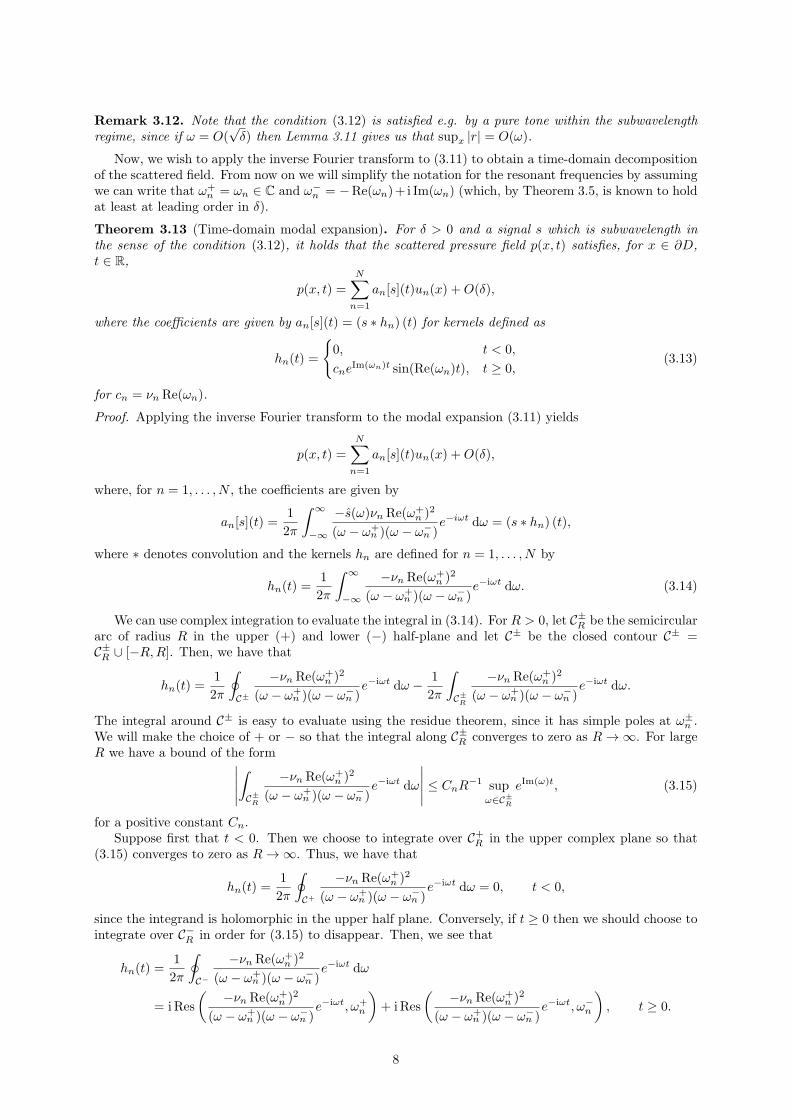
Figure 5: The architecture considered in this work cascades the physically-derived subwavelength scattering,

extracts the instantaneous amplitude and phase before, finally, estimating the parameters of the associated natural

sound distributions.

Proof. Since ‖τ ′‖∞ ≤ c < 1, ϕ(t) = t− τ(t) is invertible and ‖ϕ′‖∞ ≥ 1− c,

∫ t2

t1

(

h(k)Pk

(t− τ(t))− h(k)Pk

(t))

dt =

∫ ϕ(t2)

ϕ(t1)

h(k)Pk

(t)1

ϕ′(ϕ−1(t))dt−

∫ t2

t1

h(k)Pk

(t) dt

=

∫

I1−I2

h(k)Pk

(t)1

ϕ′(ϕ−1(t))dt+

∫ t2

t1

h(k)Pk

(t)τ ′(ϕ−1(t))

ϕ′(ϕ−1(t))dt,

for some intervals I1, I2 ⊂ R, each of which has length bounded by ‖τ‖∞. Now, define the constant

C2 := supk∈{1,...,kmax}

supPk∈{1,...,N}k

supx∈(0,∞)

(1− c)∣

∣

∣h(k)Pk

(x)∣

∣

∣ <∞.

Finally, we can compute that

〈a(k)Pk[s]〉(t1,t2) − 〈a(k)Pk

[Tτs]〉(t1,t2) =1

t2 − t1

∫ ∞

−∞

s(u)

∫ t2

t1

(

h(k)Pk

(t− u− τ(t))− h(k)Pk

(t− u))

dt du

=1

t2 − t1

∫ ∞

−∞

s(u)

(∫

I1−I2

h(k)Pk

(t− u)1

ϕ′(ϕ−1(t− u))dt+

∫ t2

t1

h(k)Pk

(t− u)τ ′(ϕ−1(t− u))

ϕ′(ϕ−1(t− u))dt

)

du,

meaning that

∣

∣

∣〈a(k)Pk[s]〉(t1,t2) − 〈a(k)Pk

[Tτs]〉(t1,t2)∣

∣

∣ ≤ 1

t2 − t1‖s‖1

[

2‖τ‖∞C2 + (t2 − t1)C2‖τ ′‖∞]

.

Remark 4.8. Lemma 4.7 shows that temporal averages are approximately invariant to translations if thelength of the window is large relative to the size of the translation (i.e. if t2 − t1 ≫ ‖τ‖∞).

5 Representation of natural sounds

Extracting meaning from the representation of a sound, beyond elementary statements about which tonesare more prolific at different stages, is difficult. In this section, we propose a novel approach tailored tothe class of natural sounds which exploits their observed statistical properties.

5.1 Properties of natural sounds

Let us briefly summarise what has been observed about the low-order statistics of natural sounds [22–25].For a sound s(t), let aω(t) be the component at frequency ω (obtained e.g. through the application of aband-pass filter centred at ω). Then we can write that

aω(t) = Aω(t) cos(ωt+ φω(t)),

12

where Aω(t) ≥ 0 and φω(t) are the instantaneous amplitude and phase, respectively. We view Aω(t) andφω(t) as stochastic processes and wish to understand their statistics.

It has been widely observed that several properties of the frequency components of natural soundsvary according to the inverse of the frequency. In particular, it is well known that the power spectrum(the square of the Fourier transform) of the amplitude satisfies a relationship of the form

SAω(f) = |Aω(f)|2 ∝ 1

fγ, 0 < f < fmax, (5.1)

for a positive parameter γ (which often lies in a neighbourhood of 1) and some maximum frequency fmax.Further, this property is independent of the frequency band that is studied [24].

Consider the log-amplitude, log10Aω(t). It has been observed that for a variety of natural sounds(including speech, animal vocalisations, music and environmental sounds) the log-amplitude is locallystationary. Suppose we normalise the log-amplitude so that it has zero mean and unit variance, giving aquantity that is invariant to amplitude scaling. Then, the normalised log-amplitude averaged over sometime interval [t1, t2] has a distribution of the form [25]

pA(x) = β exp(βx− α− eβx−α), (5.2)

where α and β are real-valued parameters and β > 0. Further, this property is scale invariant in thesense that it is true irrespective of the scale over which the temporal average is taken. It also known thatthe curves for different frequency bands fall on top of one another, meaning that pA does not depend onω (the frequency band).

Further, the power spectrum Sφωof the instantaneous phase also satisfies a 1/f -type relationship,

of the same form as (5.1). On the other hand, the instantaneous phase is non-stationary (even locally),making it difficult to describe through the above methods. A more tractable quantity is the instantaneousfrequency (IF), defined as

λω =dφωdt

.

It has been observed that λω(t) is locally stationary for natural sounds and the temporal mean of itsmodulus satisfies a distribution pλ of the form [24]

pλ(x) ∝ (ζ2 + x2)−η/2, (5.3)

for positive parameters ζ and η > 1.

5.2 Representation algorithm

For a given natural sound, we wish to find the parameters that characterise its global properties, accordingto (5.1)–(5.3). Given a signal s we first compute the convolution with the band-pass filter hn to yield thespectral component at the frequency Re(ωn), given by

an[s](t) = An(t) cos(Re(ωn)t+ φn(t)).

We extract the functions An and φn from an[s] using the Hilbert transform [24,34,35]. In particular, wehave that

an[s](t) + iH(an[s])(t) = an[s](t) +i

π

∫ ∞

−∞

an[s](u)

t− udu = An(t)e

i(Re(ωn)t+φn(t)),

from which we can extract An and φn by taking the complex modulus and argument, respectively.

Remark 5.1. It is not obvious that the Hilbert transform H(an[s]) is well-defined. Indeed, we mustformally take the principal value of the integral. For a signal that is integrable and has finite support,H(an[s])(t) exists for almost all t ∈ R.

Given the functions An and φn, the power spectra SAn(f) and Sφn

(f) can be computed by applyingthe Fourier transform and squaring. We estimate the relationships of the form (5.1) by first averaging theN power spectra, to give SA(f) :=

1N

∑

n SAn(f) and Sφ(f) :=

1N

∑

n Sφn(f) before fitting curves f−γA

13

‘

(a) A histogram of the normalised time-averagedlog-amplitude, fitted to a distribution of the form(5.2).

(b) A histogram of the normalised time-averagedinstantaneous frequency, fitted to a distributionof the form (5.3).

(c) The averaged (over different frequency bands)power spectra of the instantaneous amplitude, fit-ted to a distribution of the form (5.1).

100

101

102

10-15

10-14

10-13

(d) The averaged (over different frequency bands)power spectra of the instantaneous phase, fittedto a distribution of the form (5.1).

Figure 6: The fitted distributions for a trumpet playing a single note.

and f−γφ using least-squares regression. We estimate the parameters of the probability distributions(5.2) and (5.3) by normalising both log10An(t) and λn(t) so that

〈log10An〉 = 0, 〈(log10An)2〉 = 1,

and similarly for λn(t), before repeatedly averaging the normalised functions over intervals [t1, t2] ⊂ R.Curves of the form (5.2) and (5.3) are then fitted to the resulting histograms (which combine the temporalaverages from different filters n = 1, . . . , N and different time intervals [t1, t2]) using non-linear least-squares optimisation.

5.3 Discussion

The observations of Section 5.1 give us six coefficients (γA, α, β, γφ, ζ, η) ∈ R6 that portray global proper-

ties of a natural sound. Table 1 shows some examples of these parameters, estimated using the approachdescribed in Section 5.2. Our hypothesis is that these parameters capture, in some sense, the quality of

trumpet

violin

cello

thunder

bab

yspeech

adultspeech

runningwater

crow

call

γA 1.767 1.563 1.528 1.415 1.763 1.808 1.466 1.571α 1.244 0.375 0.284 0.474 0.517 0.528 0.336 0.649β 2.390 0.783 0.841 0.596 0.747 0.894 0.484 0.896γφ 0.763 0.871 0.6977 0.446 1.192 1.125 1.088 0.908

ζ (×10−6) 2.878 3.433 6.1149 6.322 4.773 5.176 5.200 4.212η 8.579 11.824 8.679 8.315 9.660 9.358 9.290 10.475

Table 1: Values of the estimated distribution parameters for different samples of natural sounds.

14

a signal. Thus, incorporating these parameters into the representation of a signal, alongside e.g. tem-poral averages (4.2), will improve the ‘perceptual’ abilities of any classification algorithm based on thisrepresentation. The space of natural sounds that is characterised by the six parameters is likely to havea highly non-trivial (and non-Euclidean) structure which will need to be learnt from data, cf. [36, 37].

6 Concluding remarks

We have studied an array of subwavelength resonators that has similar dimensions to the cochlea andmimics its biomechanical properties. We proved, from first principles, that the pressure field scatteredby this structure satisfies a modal expansion with spatial eigenmodes and gammatone time dependence.We, then, explored how these basis functions could be used as kernels in a convolutional signal processingroutine. In particular, we proposed an algorithm for extracting meaningful global properties from theband-pass coefficients tailored to the class of natural sounds.

An advantage of two-step approach (physical scattering followed by neural processing) is that thesubtleties of the auditory system can be readily incorporated, e.g. the non-linear amplification thattakes place in the cochlea [38]. This work studied linear representations of signals followed by a non-linear algorithm for extracting the natural sound parameters. While analyses of non-linear networks (i.e.with the activation function different from the identity) have been conducted in other settings [32, 33],an amplification mechanism based on a compressive non-linearity can be incorporated directly into theresonator-array model, as studied in [1, 2].

Acknowledgements

The numerical experiments in this work were carried out on a variety of sound recordings from theUniveristy of Iowa’s archive of musical instrument samples1 and the McDermott Lab’s natural soundsstimulus set2. The code used for this study is available for download from github3.

References

[1] H. Ammari and B. Davies. Mimicking the active cochlea with a fluid-coupled array of subwavelengthHopf resonators. Proc. R. Soc. A, 476(2234):20190870, 2020.

[2] M. Rupin, G. Lerosey, J. de Rosny, and F. Lemoult. Mimicking the cochlea with an active acousticmetamaterial. New J. Phys., 21:093012, 2019.

[3] H. Ammari and B. Davies. A fully-coupled subwavelength resonance approach to filtering auditorysignals. Proc. R. Soc. A, 475(2228):20190049, 2019.

[4] T. Duke and F. Julicher. Critical oscillators as active elements in hearing. In G. A. Manley, R. R.Fay, and A. N. Popper, editors, Active Processes and Otoacoustic Emissions in Hearing, pages 63–92.Springer, New York, 2008.

[5] B. S. Joyce and P. A. Tarazaga. Developing an active artificial hair cell using nonlinear feedbackcontrol. Smart Mater. Struct., 24(9):094004, 2015.

[6] B. S. Joyce and P. A. Tarazaga. Mimicking the cochlear amplifier in a cantilever beam using nonlinearvelocity feedback control. Smart Mater. Struct., 23(7):075019, 2014.

[7] C. F. Babbs. Quantitative reappraisal of the Helmholtz-Guyton resonance theory of frequency tuningin the cochlea. J. Biophys., 2011:1–16, 2011.

[8] V. Leroy, A. Bretagne, M. Fink, H. Willaime, P. Tabeling, and A. Tourin. Design and characterizationof bubble phononic crystals. Appl. Phys. Lett., 95(17):171904, 2009.

[9] V. Leroy, A. Strybulevych, M. Scanlon, and J. Page. Transmission of ultrasound through a singlelayer of bubbles. Eur. Phys. J. E, 29(1):123–130, 2009.

1theremin.music.uiowa.edu/MIS.html2mcdermottlab.mit.edu/svnh/Natural-Sound/Stimuli.html3github.com/davies-b/nat-sounds

15

[10] R. F. Lyon. Human and machine hearing. Cambridge University Press, 2017.

[11] J. F. Alm and J. S. Walker. Time-frequency analysis of musical instruments. SIAM Rev., 44(3):457–476, 2002.

[12] L. Cohen. Time-frequency analysis. Prentice Hall, Englewood Cliffs, NJ, 1995.

[13] S. Mallat. A wavelet tour of signal processing. Academic Press, San Diego, 1998.

[14] I. Daubechies. Ten lectures on wavelets. SIAM, Philadelphia, 1992.

[15] X. Yang, K. Wang, and S. A. Shamma. Auditory representations of acoustic signals. IEEE T.Inform. Theory, 38(2):824–839, 1992.

[16] J. J. Benedetto and A. Teolis. A wavelet auditory model and data compression. Appl. Comput.Harmon. A., 1(1):3–28, 1993.

[17] J. Anden and S. Mallat. Deep scattering spectrum. IEEE T. Signal Proces., 62(16):4114–4128, 2014.

[18] E. C. Smith and M. S. Lewicki. Efficient auditory coding. Nature, 439(7079):978–982, 2006.

[19] M. J. Hewitt and R. Meddis. A computer model of amplitude-modulation sensitivity of single unitsin the inferior colliculus. J. Acoust. Soc. Am., 95(4):2145–2159, 1994.

[20] R. D. Patterson, I. Nimmo-Smith, J. Holdsworth, and P. Rice. APU report 2341: An efficientauditory filterbank based on the gammatone function. Applied Psychology Unit, Cambridge, 1988.

[21] A. Bell and H. P. Wit. Cochlear impulse responses resolved into sets of gammatones: the case forbeating of closely spaced local resonances. PeerJ, 6:e6016, 2018.

[22] F. E. Theunissen and J. E. Elie. Neural processing of natural sounds. Nat. Rev. Neurosci., 15(6):355–366, 2014.

[23] R. F. Voss and J. Clarke. ‘1/f noise’ in music and speech. Nature, 258(5533):317–318, 1975.

[24] H. Attias and C. E. Schreiner. Temporal low-order statistics of natural sounds. In M. C. Mozer,M. Jordan, and T. Petsche, editors, Advances in neural information processing systems 9, pages27–33, Cambridge, MA, 1997. MIT Press.

[25] H. Attias and C. E. Schreiner. Coding of naturalistic stimuli by auditory midbrain neurons. In M. C.Mozer, M. Jordan, M. Kearns, and S. S, editors, Advances in neural information processing systems10, pages 103–109, Cambridge, MA, 1998. MIT Press.

[26] H. Ammari, B. Fitzpatrick, H. Kang, M. Ruiz, S. Yu, and H. Zhang. Mathematical and computa-tional methods in photonics and phononics, volume 235 of Mathematical Surveys and Monographs.American Mathematical Society, Providence, 2018.

[27] H. Ammari, B. Fitzpatrick, H. Lee, S. Yu, and H. Zhang. Double-negative acoustic metamaterials.Q. Appl. Math., 77(4):767–791, 2019.

[28] I. Gohberg and J. Leiterer. Holomorphic operator functions of one variable and applications: methodsfrom complex analysis in several variables, volume 192 of Operator Theory Advances and Applica-tions. Birkhauser, Basel, 2009.

[29] H. Ammari, B. Davies, and S. Yu. Close-to-touching acoustic subwavelength resonators: eigenfre-quency separation and gradient blow-up. arXiv preprint arXiv:2001.04888, 2020.

[30] H. Ammari, B. Davies, H. Lee, E. O. Hiltunen, and S. Yu. Exceptional points in parity–time-symmetric subwavelength metamaterials. arXiv preprint arXiv:2003.07796, 2020.

[31] S. T. Neely and D. Kim. A model for active elements in cochlear biomechanics. J. Acoust. Soc. Am.,79(5):1472–1480, 1986.

[32] J. Bruna and S. Mallat. Invariant scattering convolution networks. IEEE Trans. Pattern Anal.Mach. Intell., 35(8):1872–1886, 2013.

16

[33] S. Mallat. Group invariant scattering. Comm. Pure Appl. Math., 65(10):1331–1398, 2012.

[34] J. Flanagan. Parametric coding of speech spectra. J. Acoust. Soc. Am., 68(2):412–419, 1980.

[35] B. Boashash. Estimating and interpreting the instantaneous frequency of a signal. i. fundamentals.Proc. IEEE, 80(4):520–538, 1992.

[36] C. R. Qi, H. Su, K. Mo, and L. J. Guibas. Pointnet: Deep learning on point sets for 3d classificationand segmentation. In Proc. computer vision and pattern recognition, IEEE, pages 652–660, 2017.

[37] C. R. Qi, L. Yi, H. Su, and L. J. Guibas. Pointnet++: Deep hierarchical feature learning on pointsets in a metric space. In Advances in neural information processing systems, pages 5099–5108, 2017.

[38] A. Hudspeth. Making an effort to listen: mechanical amplification in the ear. Neuron, 59(4):530–545,2008.

17