Nonlinear Studies Nonlinear StudiesVol. 17, No. 1, pp. 1-13, 2010 ©I&S Publishers

Florida, USA, 2010

A bifurcation theorem for Darwinian matrix models

J. M. Cushing

Department of MathematicsInterdisciplinary Program in Applied Mathematics617 N Santa RitaUniversity of ArizonaTucson AZ 85721E-mail: cushing@math.arizona.edu

Abstract. Matrix models are widely used to describe the discrete time dynamics of structured populations(i.e., biological populations in which individuals are classified into discrete categories such as age, size,etc.). A fundamental biological question concerns population extinction and persistence, i.e., the stability orinstability of the extinction state versus the existence of stable positive equilibria. A fundamental bifurcationtheorem provides one general answer to this question, using the inherent population growth rate r as abifurcation parameter, by asserting the existence a continuum of positive equilibria that bifurcates fromthe extinction state at r = I. Moreover, stability of the bifurcating non-extinction equilibria is determinedby the direction of bifurcation (at least near the bifurcation point). Evolutionary game theoretic methodsgeneralize structured population dynamic models so as to include the dynamics of (mean) phenotypic traitssubject to natural selection. The resulting Darwinian matrix model describes both the structured populationdynamics and the evolutionary trait dynamics and the way in which they interplay. Here we generalize thefundamental bifurcation theorem for structured population dynamics to Darwinian matrix models. We givetwo applications.

1 Introduction

A matrix model for the discrete time dynamics of a structured population has the form [ 11, 13|

x{t+\)=P{x{t))xit) (1.1)

where the in x m projection matrix P is nonnegative and t E Z+ = {0, 1,2, • • •}, i : Z+ ^ /?'". Here R'" ism-dimensional Euclidean space . (More will be assumed about P below.) The column vector X- is a vectorof population numbers or densities of individuals lying in in disjoint classes or categories and to be of

" 2008 Maihciiialics Subject Classification: 92D15; 39A11.Keywords: Structured population dynamies; discrete time dynamieal systems; Darwinian dynamics: equilibrium; stability; bi-

furcation; exchange ol stability.

2 J. M. Cushing

biological interest must, therefore, lie in the closure R'^ of the positive cone R'!^. Equilibrium states arevectors x satisfying x — P{x)x and include the trivial or extinction equilibrium i = Ô.

A non-negative matrix is primitive if it is irreducible and has a strictly dominant eigenvalue. We makethe following assumptions concerning the projection matrix P{x) = {pij (x)). Here, as throughout, Q. denotesan open neighborhood of the origin Ô G R'".

HI: < jc e Ä'̂ and/'(je)je = Ô imply i = Ô[ P{x) is primitive for all i e fí.

Let r = r{x) denote the strictly dominant, simple and positive eigenvalue of P{x) (whose existence followsfrom Perron-Frobenius theory). Then reC^{ü.^ R\^).The number X = r(Ô) is called the inherent growthrate. Normalizing the entries of P with respect to r(Ô), we write the matrix (1.1) equation as

x{t + l) = XQ{x{t))x{t) (1.2)

where the normalized projection matrix Q{x) = {qij{x)) also satisfies HI. Note that 1 is the dominant eigen-value of 0(0).

A pair {\,x) e /?' X Q is called an equilibrium pair of the matrix model (1.2) if

x = XQ{x)x. (1.3)

The extinction equilibrium pair (A.,0) is an equilibrium pair for all X G RK If (A,,x) is an equilibrium pairand i f i i s a locally asymptotically stable equilibrium of the matrix equation (1.2) (or equivalently of (1.1)with P = XQ), then we say that the pair (À,jc) is stable. Since the Jacobian associated with (1.2) evaluatedat an extinction equilibrium pair is ^ô(Ô), which has dominant eigenvalue A,, the linearization principle [6|establishes part (a) of the following theorem. Parts (b) and (c) follow from Theorems 1.2.4 and 1.2.5 in | 3 | .

Theorem 1. [3] Assume the matrix Q{x) in the matrix equation (1.2 ) satisfies HI and that 1 is the dominanteigenvalue of 0(0).

(a) The extinction equilibrium pair {X,Ô) is stable for A, < 1 and is unstable for X, > 1.(b) There exists a continuum C of (positive) equilibrium pairs (A,, i ) € /?+ x R'^_ of the matrix model (1.2)

that contains the extinction pair (1,0) in its closure.(c) If C bifurcates to the right from (1,0), then the equilibrium pairs on C near (1,0) are stable. If C

bifurcates to the left from (1,0), then the equilibrium pairs on C near (1,0) are unstable.

In part (c), bifurcation to the right (left) means that in a neighborhood of ( 1,Ô) the equilibrium pairs (i, X)from C satisfy X> I (A. < 1). This is the familiar exchange of stability principle that occurs for transcriticalbifurcations [7].

Theorem 1 applies to the matrix equation (1.1) with P{Jc) = XQ{x) where X = r(Ô) is the dominanteigenvalue of the inherent projection matrix P(Ô).

The direction of bifurcation in (c), and hence the stability of the continuum near bifurcation, is deter-mined by the sign of the quantity

A Bifurcation Theorem for Darwinian Matrix Models 3

K=-w'''[V( pij{Ô)v]v (1.4)

(|3|, Theorem 1.2.5). Here the superscript'T" denotes transpose and the gradient Vf of pij{x) with respectto X is a row /n-vector. The vectors w'^ and v are the (positive) left and right eigenvectors of P{Ô) associatedwith the dominant eigenvalue 1, normalized so that w' v = I. If K is negative, the bifurcation is to the rightand, by Theorem 1, is therefore stable. If K is negative, then the bifurcation is to the left and unstable.

The most common assumption made in population models is that density effects are negative feedbackeffects, i.e., the derivatives appearing in the gradients Vf p,y are negative (or zero). Clearly this impliesK > 0 and a stable bifurcation to the right. Only if sufficiently large positive feedbacks occur (i.e., there isat least one positive derivative of sufficient magnitude from one of the gradients Vf Pij{Ö)) will an unstablebifurcation to the left occur. A positive feedback term is called an Allee effect in population biology. In otherwords, Allee effects of sufficient magnitude lead to unstable bifurcations to the left. In the absence of Alleeeffects, the bifurcation is to the right and hence stable.

The continuum C in Theorem I in known to exist globally in the sense that it connects to the boundaryon which the matrix model is defined, i.e., it connects to the set {+°°} x (dCiriR'!^), where dO. denotesthe boundary of Q. (Theorem 1.2.4 in [3]). In most applications, the nonlinearities in (1.2) are defined onthe closure of the positive cone, i.e., R"[ C H in HI. In this case, along the continuum of equilibrium pairs(k.x) either the component X is unbounded or the magnitude |i | is unbounded in /?.',. (or both). In the formercase, there exists at least one non-extinction equilibrium from each X> 1. In specific applications, one canoften determine which of these properties the equilibrium pairs possess by a careful consideration of theequilibrium equations.

2 Darwinian Matrix Models

In 110] Vincent and Brown develop a theory that extends population dynamic models, and in particularmatrix models, to include the dynamics of an evolving (mean) phenotypic trait (that possesses a heritablecomponent) under the influence of natural selection. Under the assumption that the entries in the projectionmatrix P depend on such a trait, as quantified by a scalar u, we write P = P{x,ii) and r = r{x,u). Theso-called Darwinian dynamics o f i and u are described by the equations | lOJ

(2.1b)r{x,u)

Here r,, denotes the partial derivative of r with respect to u. The quantity a~ is the variance of the trait (fromits mean u) that occurs in the population at each time. It is therefore a measure of the speed of evolution.

When there is no evolution a" = 0, the Darwinian model (2.1) reduces to the population dynamic model(1.1) in which the trait is fixed, say ii{t) = u*. In this case. Theorem I applies with P{x) = XQ{.x,ii*) andX = r(Ô, u*). In this section we extend Theorem I to the Darwinian model (2.1 ) when evolution does occurio'- > 0).

We make the following assumptions concerning the projection matrix P{x,u) — (/7//(i,i/)). Here Udenotes an open interval in /?'.

4 J. M. Cushing

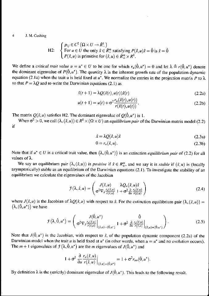
C Pij eC~{ÇlxU^ Ri)H2: < For tí e í/ the only x G R'" satisfying P{x, u)x = Ô\sx-Ô

[ P{x.,u) is primitive for {x,u) 6 R'!^ x RK

We define a critical trait value u = u* G U to be one for which /-«(Ô,«*) = O and let À = r{Ô,u*) denotethe dominant eigenvalue of P{Ô,u*). The quantity A, is the inherent growth rate of the population dynamicequation (2. la) when the trait u is held fixed at u*. We normalize the entries in the projection matrix PtoXso that P = XQ and re-write the Darwinian equations (2.1) as

x{t + l)=XQ(x{t),u{t))x{t) (2.2a)

The matrix Q{Jc,u) satisfies H2. The dominant eigenvalue of ß(0,M*) is I.When a-̂ > 0, we call {X, {x, u)) eR^ x{D.xU) an equilibrium pair of the Darwinian matrix model (2.2)

if

x^XQ{x,u)x (2.3a)

O = r,,(x,«). (2.3b)

Note that if M* € {/ is a critical trait value, then (A,, (Ô, u*)) is an extinction equilibrium pair of (2.2) for allvalues of X.

We say an equilibrium pair {X,{Jc,u)) is positive if i € R'J^, and we say it is stable if {x,u) is (locallyasymptotically) stable as an equilibrium of the Darwinian equations (2.1). To investigate the stability of anequilibrium we calculate the eigenvalues of the Jacobian

[ K^^u) XQu{x,u)x \

U ## (2.4,where J{x,u) is the Jacobian of XQ{x,u) with respect to x. For the extinction equilibrium pair (X, {x,u)) ={X,{Ô,u*)) we have

7(Ô,«*) Ô,2 d '•„{.x;u) (2.5)

Note that 7(0,«*) is the Jacobian, with respect to x, of the population dynamic component (2.2a) of theDarwinian model when the trait u is held fixed at u* (in other words, when u = ti* and no evolution occurs).The m+ I eigenvalues of J/ (A,,Ô,i<*) are the m eigenvalues of 7(0,«*) and

I+O^du r[Jc,u)

By definition À, is the (strictly) dominant eigenvalue of 7(0,«*). This leads to the following result.

A Bilurcaiion Theorem lor Darwinian Malrix Models .5

Theorem 2. Assume H2 and that ii* € ¿/ is a critical trait. For A, € /?.',. the extinction equilibrium pair(X, (Ô,i<*)) is unstable if /-uu(Ô,t<*) > 0. If ruu{Ô,u*) < 0, then the extinction equilibrium pair (A,, (Ô,i/*))is

(a) unstable if X, > I(b) stable if A, < I provided the speed of evolution a^ is sufficiently small, specifically if

a-< Î . (2.6)ruu{O,u*)

We point out that the derivation of the Darwinian equation (2.1b) (or (2.2b)) requires that O'̂ is small[101, so that this requirement in part (b) is not restrictive.

3 A Bifurcation Theorem

In Theorem 2, the extinction equilibrium loses stability as A, increases through I provided r,,i,{Ô, u*) < 0, i.e.,provided r{Ô,u) has a local maximum as a function of the trait u at the critical trait value u = u*. Since thisdestabilization occurs because an eigenvalue of the Jacobian leaves the unit circle at I, we expect that thereis an equilibrium bifurcation at A, = I. We investigate this possibility by making use of Theorem I.

We assume that the equilibrium equation (2.3b) can be solved for u as a function of i .

{ Let u* € Í/ be a critical trait. Assume there exists a functionveC-{N,U) such that n,{x,v{x)) = 0, •u(Ô) = u*, whereN C /?'" is an open neighborhood of Ô.

The following as.sumption is (by the implicit function theorem) sufficient to guarantee that H3a holds:

H3b: Let u* G Í/ be a critical trait such that r,,,,(Ô,i<*) / 0.

Under H3a the equilibrium equations (2.3) reduce to

x = XQ{x,\){x))x (3.1)

to which Theorem 1 applies with Q{x) and Í2 replaced by Q{x.,v{x)) and A' respectively. The bifurcatingcontinuum C of positive equilibrium pairs (A,,i) of this equilibrium equation guaranteed by Theorem l(b)produces a continuum <í = {(A,, {x, u)) \ (A,,Â) E C,LI = t)(i)} of positive equilibrium pairs of the Darwinianmodel (2.1 ). This proves part (a) of the following result.

Theorem 3. Assume u* G Í/ is a critical trait. Assume H2 and H3a.(a) There exists a continuum € of (positive) equilibrium pairs (A., (x, «)) G /?.',. x (/?"! x U) of (2.1 ) that

contains the extinction pair ( 1, (0, u*)) in its closure.Suppose the stronger assumption H3b holds.(b) If r,i,i[0,11*) > 0, then near the bifurcation point the positive equilibrium pairs are unstable.

6 J. M. Cushing

(c) Suppose r,,i,{Ô,u*) < O and a^ is small (i.e., (2.6) holds). Near the bifurcation point the positiveequilibrium pairs are stable if the bifurcation is to the right, i.e., if

K*â-vv^[V,.p,XÔ,«*)v]v>0 (3.2)

and are unstable if the bifurcation is to the left, i.e., if K* < 0.

Proof. We have only parts (b) and (c) left to prove. Near the bifurcation point (A,,(i,«)) = (I, (Ô,M*)) thesmoothness assumption H2 guarantees that we can parameterize the bifurcating equilibria :

(3.3)

for small positive £ ~ 0 [3]. Here v is a positive right eigenvector of P(Ô,u*) associated with the dominanteigenvalue 1. We obtain the formula

". = -̂ #̂? (3.4,( 0 * )

from a differentiation of r,,(jc(e), t<(e)) = 0 with respect to e followed by an evaluation at e = 0. The param-eterization (3.3) allows us, in turn, to parameterize the Jacobian J/ (A,(e),i(e),a(e)) and its eigenvalues. Ate = 0 the spectrum of the Jacobian (2.5) are the eigenvalues of 7(0,«*) and I -\-o~r,,i,{Ô,u*). By continuity,as e ̂ 0 the spectrum of J/(>,(e),i(e),M(e)) approaches that of J/ (1,0,«*). Thus, if r,,,,(Ô,«*) > 0, the Ja-cobian J (A,(£),jc(e), «(e)) has an eigenvalue greater than I for e ̂ 0 and, as a result, the positive equilibriaare unstable. This proves part (b).

If, on the other hand r,,,,(Ô,«*) < 0 and (2.6) holds, then I is the dominant eigenvalue of j7 ( | ,Ô,Î<*),

since by construction 1 is the dominant eigenvalue of 7(0,«*). It is thus unclear whether the eigenvalueJ7 (A,(e),jc(e),i/(e)) that approaches I does so from above or below. To answer this question we calculate thesign of the coefficient ;U| in the expansion

of the dominant eigenvalue of J7(?L(£),JC(£), «(£)). Near the bifurcation point the positive equilibrium pairsare stable if/^i < 0 and unstable \f fj] > 0.

We can use a standard perturbation (Lyapunov-Schmidt) approach to calculate a formula for^t/i. We makeuse of the expansions (3.3 ) and of the {in + 1 )-column eigenvector

associated with /j(£) in the equation

HMe),x{^),u{e))V{£)=n{£)V{£). (3.5)

Eirst, setting £ = 0 in (3.5) we obtain

A Bifurcation Theorem for Darwinian Malrix Models 7

Ô

and hence

We note in passing that the left eigenvector

V

satisfiesiT\i (3.6)

Differentiating (3.5) with respect to £ and setting e = 0, we obtain (after some algebraic re-arrangement)

d_~dz E=()

where / is the (m -f- I ) x (m -f I ) identity matrix. This equation is solvable for V\ if and only if the right handside is orthogonal to WQ, a fact that together with the orthogonality condition (3.6), implies

What remains is a calculation of the matrix ^J/(A,(e),i(e),t<(e))|g^P from (2.4) and (3.3). While tedious,this is a straightforward calculation and we omit the details. Since it is only the sign of fj\ that we wish toknow, it is enough to say that the result of the calculation is

^^\ = -k-K*

where k- is a positive quantity and, as a result, ¿ui and K* have opposite signs. Thus, if K* > 0 we concludethe bifurcation is to the right and the positive equilibria are stable. If, on the other hand, K* < 0 then thebifurcation is to the left and the positive equilibria are unstable. D

In the remarks following Theorem 1, we noted that the bifurcating continuum C connects to the boundaryon which the matrix model was defined. Similarly, the continuum of equilibrium pairs of the Darwinianmatrix model (2.3) connects to the set of {oo} x [(dNDR'".) xdu). If r = v{x) in H3a is defined on theclosure of the positive cone, i.e., if !̂J! C N, then along the continuum (Í the component X or the equilibriummagnitudes |.v'| are unbounded or the trait u approaches the boundary of U (or both). A careful considerationof the equilibrium equations in specific applications can often determine which of these alternatives occurs.It can be of interest to know that the component X is unbounded along the continuum because this impliesthe existence of at least one non-extinction equilibrium for each X> \.

8 J. M. Cushing

Suppose (À(,, {xe,Ue)) is an equilibrium pair from the continuum € with to Xe~ I. From the equilibriumequations and assumption H2 follow r{xe,Ue) = 1 and r,,(jCe,ííe) = 0. If ruu{Ô,u*) < 0 (so that an exchangeof stability bifurcation occurs by Theorem 3), then ruu{xe,Ue) < 0 near the bifurcation point. If follows thatin this case the trait component u = «<, from a bifurcating non-extinction equilibrium maximizes the growthrate r(jCe, u) (at 1) as a function of u while holding x = Xe fixed.

As a final comment, we point out that in the event of a bifurcation right bifurcation at À = I, the stabilityof the bifurcating non-extinction equilibria is guaranteed by Theorem 3 only near the bifurcation point,i.e., for X,^ 1 and equilibria {x,u) near (Ô,M*). Away from the bifurcating point, these equilibria might notbe stable. Indeed, the non-extinction equilibria might, depending on the nature of the nonlinearities in theDarwinian model, destabilize and result in periodic or chaotic oscillations. In the second application in thefollowing section, we illustrate this point.

4 Applications

4.1 A Juvenile-Adult Model

T h e m a t r i x e q u a t i o n ( 1 . 1 ) w i t h t h e 2 x 2 p r o j e c t i o n m a t r i x

)

models the dynamics of a population vector jc = col(jci ,X2) consisting of juveniles x\ and adults xo in whichthe unit of time equals the length of the juvenile maturation period. The number s\ is the juvenile survivalprobability (per unit time) and .y2 is the adult survival probability (per unit time). The term bf{x) is therecruitment rate (the number of surviving offspring per adult per unit time) when the population vector isJC. Here we normalize the population density dependent factor / so that /(Ô) = I. In this way, the constanth>O\s the inherent recruitment rate, i.e., the recruitment rate when population numbers are low (technically,x = Ô).

In this example we consider the case when recruitment processes bf depend on the trait ii, but thesurvivorships .y, do not:

(4.2)

The assumption H2 holds if

H4:0 < .y, < 1, 0 < .V2 < I.

From

r{x,u) = -,y2 + 2 \j4.'nb{u)f{x,u)

we calculate

A Bifurcation Theorem for Darwinian Matrix Models

Thus, critical traits « — u* are the critical points of ¿(«), the inherent birth rate, i.e., u* must satisfy //(«*) = 0.At such a critical trait, another differentiation yields

Finally, we assumef:,.{Ô,«) < 0 for « G Í/ and either / = I or 2 (or both).

Note that this implies K* > 0.From Theorem 3 we obtain the following results for the Darwinian juvenile-adult matrix model (2.1)

with projection matrix (4.2) under assumption H4. Here

1- 2-̂ 2 +

( I ) Critical traits «* are critical points of the inherent birth rate b{u).If b"{ti*) ^ 0, then a continuum of positive equilibrium pairs(A,, (i,«)) € /?.',. X {R\ X U) bifurcates from ( I, (Ô, «*)).

(2) If/?"(«*) < 0, then the extinction equilibrium (Ô,«*) loses stabilityas A. increases through I the positive equilibria (i, «) as stable for A, ^ I.

(3) If/?"(«*) > 0, then both the extinction equilibria and the bifurcatingpositive equilibria are unstable for A. fti I.

Note that the fundamental exchange of stability from extinction to a stable non-extinction (positive)equilibrium occurs in an evolutionary context for the Darwinian model (4.2) at critical trait values «* thatmaximize the inherent birth rate b{u). At a minimum of the birth rate, both equilibria are unstable and thenature of the long term asymptotic dynamics remains an open question.

As an illustration consider an inherent birth rate that is normally distributed as a function of the trait «and density factor / that has a Ricker form:

b{u) = b,,,exp{-u~/2b,,)

/ ( i ,« ) = exp(—C| {u)x] — C2{u)x2), Q(« ) > 0, c'j(O) + C'T(O) ^ 0.

Then the only critical point is u* = 0 and the results above imply that non-extinction equilibria bifurcatefrom the extinction equilibrium pair ((J:I,A'2),«) = ((0,0),0) at A, = 1 where

. ' ' f7~, ^A = —ÍT -f- — \ / 4.S' 1 b,,, + .S'T .2 2

The bifurcation is to the right and these equilibria are stable at least for A. <; 1.

10 J. M.Cushing

Note that the inter-class competition coefficients c,(«) play no role in these conclusions. This is be-cause they occur in higher order terms near the bifurcation point. They do, however, determine interestingproperties of the bifurcating non-extinction equilibria.

For example, a calculation using (3.4) shows

where v = col(vi, va) is a right, positive eigenvector of P{0,0), say v = co l ( l ,5 i / ( l —S2)). Thus, along thebifurcating continuum, near the bifurcation point, the trait components of the equilibria satisfy

M < 0 if c ' , ( ^ ^

a > 0 if c\ (0) + 4 (0) - ^ ^ < 0.I — S2

This has the following interpretation. The quantity

I — S2

is a measure of the total competitive intensity within the population, weighted according to the expectedamount of time a juvenile is expected to spend in each age class during its life. Then the trait components ofthe equilibria satisfy

i i < 0 if V ( 0 ) > 0

t o 0 if v/(0) < 0.

Since the normally distributed inherent rate b(u) is increasing for M < 0 and decreasing for u > 0, we see thatthe trait component u near bifurcation will be negative if i|/'(0) > 0, which implies at this trait that V|/(«) isincreasing. That is to say, both b{ii) and \|/(ÍÍ) have the same monotonicity at the equilibrium trait component.This represents a trade-off in that an increase of the trait from this equilibrium value will increase the birthrate b{u) but decrease the density factor f{x, 11). (This is in contrast to what happens for w > 0 were both b{u)and f{x, u) to decrease.) A similar analysis of the case V|/'(0) < 0 leads to the same conclusion, namely, thatthe non-extinction equilibria occur with trait components at which a trade-off occurs between the inherentbirth rate and the effect of density on recruitment.

4.2 The LPA Model and the Evolution of a Polymorphism

In [9] a Darwinian version of the three life-cycle stage matrix model is used to describe the observed popu-lation dynamics and evolution of a polymorphism in a controlled, laboratory experiment involving the beetleTriboliuin castaneum |5 | . In that experiment cultures of T. castaneum homozygous for corn oil sensitivitywere perturbed by adding homozygous wild type individuals. The observed data included population densi-ties of larvae, pupae, and adults as well as alíele frequencies obtained from genetically perturbed cultures.

A Bifurcation Theorem for Darwinian Matrix Models 11

Rael et al. [9| use a Darwinian version of the LPA model |4|. The LPA model (which has been widelysuccessful in describing and predicting the population dynamics of Triboliiim |2|) is a m = 3 dimensionalmatrix model with projection matrix

in which the components of i = col(xi ,X2,x-i) are the numbers of larval, pupal, and adult individuals.Sensitivity to com oil in T. castaneum is determined genetically by a single locus with two alíeles, a wild

and a corn oil sensitivity alíele. This sensitivity, it turns out, affects the demographic parameters /?,/;/ and/ifl (larva recruitment, larval death, and adult death rates respectively), but not the (cannibalism) coefficientsCchCpa and Cpa. Taking the mean frequency of the wild type alíele as the trait « in a Darwinian model, Raelet al. use data to determine the following relationships:

1 (4.3)

/io(«) = O.IOv--0.13v-t-0.1l.

Using a computer algebra program, we can calculate the dominant eigenvalue /•(;?,«) of

and use the result, together with (4.3) to show that «* = 0.62415 is a critical trait at which Î-,,,,(Ô,«*) =— 1.7745 < 0. According to Theorem 3 a continuum of non-extinction equilibria of the Darwinian LPAmodel bifurcates from the equilibrium (Ô,«*) at A, = 1. Because the exponential nonlinearities in the LPAmodel are decreasing functions of population densities x, (i.e., the density effects are negative feedbackeffects and there are no Allee effects), the bifurcation is to the right and stable. It follows that the bifurcatingnon-extinction equilibria are stable for at least X ̂ I and equilibria (jc, «) near (Ô, i/*).

Note that near bifurcation, the non-extinction equilibrium pairs have traits « « «* = 0.62415. This meansthat at equilibrium the population is polymorphic with a wild type gene frequency of approximately 62%.

Simulations of the Darwinian LPA model verify the existence and stability of these non-extinction equi-libria for A, > 1 close to I. For the specific parameterization (4.3), a calculation shows that X, = r(Ô,«*) =2.4490. However, simulations also show that the non-extinction equilibrium is unstable |9 | for this value ofX because a period doubling bifurcation occurs along the equilibrium continuum. In fact, 2-periodic oscil-lations, that are well approximated by the model simulation, are observed in the population data x/. On theother hand, the model predicted 2-periodic oscillations in the trait « have an amplitude around a mean near«* = 0.62415 that is too small to be observed in the genetic data, which in fact are well approximated by «*191.

12 J. M. Cushing

5 Concluding Remarks

Theorem I is a basic theorem in the theory of structured population dynamics in the sense that it deals withthe fundamental question of extinction versus survival as a function of the population's inherent growthrate X = r{Ô). The theorem treats this basic biological problem as a bifurcation question concerning thegeneral matrix model (1.1) for the dynamics of a structured population. The destabilization of the extinctionequilibrium as X increases through I results in the bifurcation of a (global) continuum of positive equilibriawhose stability near the bifurcation point depends on the direction of bifurcation.

Theorems 2 and 3 provide an extension of this bifurcation theory to an evolutionary context. Evolutionarygame theory methods provide the Darwinian matrix model (2.1) when the population dynamic projectionmatrix P now depends on a (mean) phenotypic trait that is subject to evolution by natural selection [10].The loss of stability of the extinction equilibrium and possibility of the bifurcation of positive equilibria canoccur only at critical values M = M* of the phenotypic trait, i.e., at trait values where the inherent growthrate r{Ô,u) has a critical value. Theorems 2 and 3 assert, among other things, that a bifurcation of positiveequilibria will occur, and their stability will depend on the direction of bifurcation, provided r,,u(Ô,t<) < 0 . Inthis case, which implies that the inherent growth rate r(Ô,i<) has a local maximum at the critical trait u — u*,the bifurcation result is exactly analogous to the non-evolutionary case in Theorem 1.

Evolutionary game theory was developed in the context of the concept of an evolutionary stable strategy(ESS). This concept involves the issue of additional species interacting and possibly invading a residentspecies. We do not consider this question here, except to say that the condition ri,it{xc,Ue) < 0 which holdspositive equilibria near the bifurcation point is a necessary condition of an ESS (a fact known as the ESSMaximum Principle [10|). See [11].

When r,ii,{O,u) > 0 we see from Theorems 2 and 3 that both the extinction equilibrium and the positiveequilibria near the bifurcation point are unstable. What the attractor is, in this case, remains an open question.In any case, our results show that it is not an ESS (since the ESS Maximum Principle fails to hold).

We emphasize that the stability and direction of bifurcation result in Theorem 3 is only valid in generalnear the bifurcation point. One expects (as illustrated in section 4.2), from the well known propensity fordifference equations to exhibit non-equilibrium and even chaotic dynamics, that depending on the proper-ties of the nonlinearities in the projection matrix P secondary bifurcations can occur as the result of thedestabilization of the positive equilibria as one moves along the continuum away from the bifurcation point.

References

111 H. Ca.swell, Matrix Population Models: Construction. Analysis and Interpretation, Second Edition. Sinauer Associates, Inc.Publishers, Sunderland, Massachusetts, 2001

|2 | R. F. Costantino, R. A. Desharnais, J. M. Cushing, B. Dennis, S. M. Henson, and A. A. King , The Hour beetle Tribolium asan effective tool of discovery. Advances in Ecological Research 37 (2005), 101-141

[3| J. M. Cushing, An Introduction to Structured Population Dynamics, CBMS-NSF Regional Conference .Series in AppliedMathematics, Vol. 71, SI AM, Philadelphia, 1998

|4| B. Dennis, R. A. Desharnais, J. M. Cushing, and R. F. Costantino, Nonlinear demographic dynamics: mathematical, models,statistical methods, and biological experiments. Ecological Monographs 65 (1995), 261-281

A Bifurcation Theorem for Darwinian Matrix Models 13

|51 R. A. Desharnais and R. F. Costantino, Genetic analysis ol a population of Triholium. VI I . Stability: Response to Genetic and

Demographic Perturbations, Canadian Journal of Genetics and Cylology 22 (1980), 577-589

|6| S. N. Elaydi, An Inlroduclion lo Difference Equations, third edition. Springer-Verlag, New York, 2005

|71 H. Keilhöler, Bifurcation Theory: An Introduction with Applications to PDEs, Applied Mathematical Sciences 156, Springer,

New York, 2004

|8| P. H. Rabinowitz, Some global results for nonlinear eigenvalue problems. Journal of Functional Analysis 7, No. 3 (1971),

487-513

[9] R. C. Rael, R. F. Costantino, J. M. Cushing, and T. L. Vincent, Using Stage-Structured Evolutionary Game Theory to Model

the Experimentally Observed Evolution of a Genetic Polymorphism, Evolutionary Ecology Research, 11 (2009), 141-151

110| T. L. Vincent and J. S. Brown, Evolutionary Game Theory. Natural Selection, and Darwinian Dynamics, Cambridge Univer-

sity Press, 2005

111] R. C. Rael, T. L. Vincent, and J. M. Cushing, Competitive outcomes changed by evolution, to appear in the Journal of

Biological Dynamics, 2010

The formula for ∗ on page 6 should be

∗ = −£∇0¤ + ∇00uu

£0

¤ 0 (3.2)

1

Copyright of Nonlinear Studies is the property of I & S Publishers and its content may not be copied or emailed

to multiple sites or posted to a listserv without the copyright holder's express written permission. However,

users may print, download, or email articles for individual use.