a biarc based subdivision scheme for space curve interpolation
TRANSCRIPT
Computer Aided Geometric Design 31 (2014) 656–673
Contents lists available at ScienceDirect
Computer Aided Geometric Design
www.elsevier.com/locate/cagd
A biarc based subdivision scheme for space curve
interpolation ✩
Chongyang Deng a,b, Weiyin Ma b,∗a School of Science, Hangzhou Dianzi University, Hangzhou 310018, Chinab Department of Mechanical and Biomedical Engineering, City University of Hong Kong, Kowloon, Hong Kong, China
a r t i c l e i n f o a b s t r a c t
Article history:Received 13 March 2013Received in revised form 31 October 2013Accepted 31 July 2014Available online 13 August 2014
Keywords:Geometry driven subdivisionNonlinear subdivision schemeSpace curve interpolation3D biarc interpolationSpherical curveConvexity preserving
This paper presents a biarc-based subdivision scheme for space curve interpolation. Given a sequence of space points, or a sequence of space points and tangent vectors, the scheme produces a smooth curve interpolating all input points by iteratively inserting new points and computing new tangent vectors. For each step of subdivision, the newly inserted point corresponding to an existing edge is a specified joint point of a biarc curve which interpolates the two end points and the tangents. A provisional tangent is also assigned to the newly inserted point. Each of the tangents for the following subdivision step is further updated as a linear blending of the provisional tangent and the tangent at the respective point of a circle passing through the local point and its two adjacent points. If adjacent four initial points and their initial reference tangent vectors are sampled from a spherical surface, the limit curve segment between the middle two initial points exactly lies on the same spherical surface. The biarc based subdivision scheme is proved to be G1 continuous with a nice convexity preserving property. Numerical examples also show that the limit curves are G2 continuous and fair. Several examples are given to demonstrate the excellent properties of the scheme.
© 2014 Elsevier B.V. All rights reserved.
1. Introduction
Designing a smooth interpolation curve from a given polygon by repeated subdivision is an important modeling method in Computer Aided Geometric Design. One of the classical subdivision schemes for curve interpolation is four point in-terpolatory subdivision (Dyn et al., 1987). It is simple to implement and is regarded as a significant curve subdivision scheme. Limit curves of four point interpolatory subdivision may however exhibit undesired artifacts and undulations (Marinov et al., 2005). To achieve the aim of shape preserving and artifact removing, some geometry driven schemes have emerged (Dyn et al., 1992; Marinov et al., 2005; Sabin and Dodgson, 2005; Yang, 2006; Deng and Wang, 2010;Deng and Ma, 2012). In this paper we generalize the incenter subdivision scheme (Deng and Wang, 2010) to a scheme for 3D curve interpolation with the properties of convexity preserving and artifacts removing.
One subdivision step of the incenter subdivision scheme (Deng and Wang, 2010) consists of three main stages. Firstly, for each edge, we insert a new point which is the incenter of a triangle formed by the two end points of the edge and its end tangents, i.e., a special joint point of the G1 biarc matching the two end points and tangents. Secondly, we select
✩ This paper has been recommended for acceptance by H. Prautzsch.
* Corresponding author.E-mail addresses: [email protected] (C. Deng), [email protected] (W. Ma).
http://dx.doi.org/10.1016/j.cagd.2014.07.0030167-8396/© 2014 Elsevier B.V. All rights reserved.

C. Deng, W. Ma / Computer Aided Geometric Design 31 (2014) 656–673 657
a provisional tangent for each point such that there exists a G1 continuous circular arc spline interpolating the points and their provisional tangent vectors. If the tangents remain the same for the next level of subdivision, the limit curve would be the biarc spline curve which is a G1 curve interpolating all initial points. Finally, to obtain a G2 limit curve, we rotate the provisional tangent for each of the refined points according to the radii of two adjacent circular arc segments, i.e., all tangents are updated for the next level of subdivision. Note that this applies to the tangents at the points inherited from the previous step, as well as the new ones. If the old tangents were not modified, the scheme would be a Hermite one, probably G1, but certainly not G2.
To extend the incenter subdivision scheme to 3D , we need to compute newly inserted points (Stage I), their provisional tangents (Stage II), and updated tangents for the next level of subdivision (Stage III), all in 3D . The formulation of 2D biarc interpolation was extended to 3D in Sharrock (1987), Hoschek (1992). So the first and the second stages of the incenter subdivision scheme, i.e., the rule of adding new point as a special joint point of the G1 biarc matching the two end points and tangents and the rule of defining a provisional tangent for each of the inserted points such that there exists a G1
continuous circular arc spline interpolating the points and their provisional tangent vectors, can be easily generalized to the 3D case. The crux of the generalization thus lies in how to update tangents in 3D for the next level of subdivision since there is no trivial solution to rotate the tangents in 3D space which yields a well-behaved limit curve.
Given three points p1, p2, p3 sampled on a G2 curve p(t) in 2D or 3D , when p1 and p3 moving closer and closer to p2, the discrete tangent at p2 should be closer and closer to the tangent of p(t) at p2 and the radius of the arc segment interpolating p1, p2, p3 should also be closer and closer to the curvature radius of p(t) at p2. Similarly, for a subdivision scheme generating G2 limit curves, the discrete curve formed by refined points should be smoother and smoother with the level of subdivisions higher and higher. At the same time, the discrete tangent and curvature at each refined point should also gradually converge to those of the limit curve. Inspired by these facts, we define each of the new tangents for the next level of subdivision as a linear blending of its provisional tangent and the tangent of the circle passing through the respective point and its two adjacent points. This method is much simpler than the rotation-based method used in the incenter subdivision scheme and numerical examples show that the limit curves produced by this method are also attractive. Furthermore, because 3D biarc curve lies on a spherical surface, the scheme can generate spherical curve segment if adjacent four initial points and their tangents are sampled from a spherical surface. Theoretical analysis shows that the proposed 3D biarc-based subdivision scheme is convexity preserving and the limit curve is G1 continuous. Many numerical examples also show that the limit curves are fair curves with G2 continuity.
The rest of this paper is organized as follows. In Section 2, we briefly highlight the background knowledge of biarc in-terpolation. The proposed biarc based subdivision scheme is introduced in Section 3. The property of generating spherical curves by the proposed scheme is presented in Section 4. The convexity preserving property of the proposed scheme is proved in Section 5. Further smoothness analysis of the scheme is presented in Section 6. Section 7 provides some ex-perimental examples to demonstrate the excellent properties of the scheme. Some concluding remarks can be found in Section 8.
2. Theory of biarc curve interpolation
In this section, we briefly highlight the theory of interpolating G1 Hermite data using a biarc curve. Both planar case and spatial case are discussed. To be consistent with the rule of subdivision, we let a 2D or 3D biarc interpolate the local i-th G1 Hermite data {pk
i , Tki ; pk
i+1, Tki+1}, where k represents the level of subdivision, pk
i , pki+1 are two adjacent points, and T k
i
and T ki+1 are their unit tangent vectors, respectively. See Figs. 1 and 2 for 2D and 3D cases, respectively.
2.1. Planar biarc formulation
A biarc curve consists of two circular arc segments that interpolate two end points and the end tangents in a G1 fashion. Planar biarcs appeared in the engineering design literature as early as the 1930s (Sandel, 1937). They were then studied in 1970s (Bézier, 1972; Bolton, 1975; Sabin, 1977) and research has continued in Piegl et al. (2009 and reference therein).
Given the i-th local G1 Hermite data {pki , T
ki ; pk
i+1, Tki+1}, let αk
i and βki be the angles from T k
i to pki pk
i+1 and from pki pk
i+1
to T ki+1, respectively, pk+1
2i+1 be the joint point of the biarc and U k+12i+1 be the common unit tangent vector at pk+1
2i+1, and θ be the angle from T k
i to U k+12i+1, θ is then a free parameter which can be used to control the shape of the biarc (see Fig. 1).
For the planar case, an angle is positive if it is counterclockwise and negative if it is clockwise. If slope angles αki and
βki have the same sign, the biarc curve is C-shaped; otherwise the biarc curve is S-shaped. For the free parameter θ , it
is suggested that for many cases, θ = αki (see Fig. 1(a)) for C-shape biarc curves and θ = 1
2 · (3αki − βk
i ) (see Fig. 1(b)) for S-shape biarc curves are good selections (Sabin, 1977). In fact, for C-biarc curve with θ = αk
i , the joint point pk+12i+1 is the
incenter of the triangle formed by pki pk
i+1 and T ki , T k
i+1 (in the case that the radial lines pki T k
i and T ki+1 pk
i+1 intersect), the incenter subdivision scheme (Deng and Wang, 2010) is developed based on this fact.
2.2. Spatial biarc interpolation
For the 3D case, we assume that vectors T ki , T k
i+1, pki+1 − pk
i are non-coplanar. 3D circular biarc curves are consid-
ered in Hoschek (1992), Sharrock (1987). They show that a 3D biarc curve, which interpolates 3D G1 Hermite data

658 C. Deng, W. Ma / Computer Aided Geometric Design 31 (2014) 656–673
Fig. 1. Illustration of 2D biarc curves: (a) a C-shape curve; (b) an S-shape curve.
Fig. 2. Illustration of 3D biarc curves: (a) a C-shape curve; (b) an S-shape curve.
{pki , T
ki ; pk
i+1, Tki+1}, lies on a spherical surface whose center is the intersection of three planes. One plane passes through
the midpoint of pki pk
i+1 and is perpendicular to pki pk
i+1. The other two planes pass through the two end points pki , p
ki+1 and
are perpendicular to the two end tangents T ki , T k
i+1, respectively. It is easy to see that
Lemma 2.1. If the G1 Hermite data {pki , T
ki ; pk
i+1, Tki+1} is sampled from a spherical surface, the resulting 3D biarc curve lies on this
spherical surface.
Remark 2.2. If the given G1 Hermite data {pki , T
ki ; pk
i+1, Tki+1} is co-circular, the sphere is not uniquely defined. However,
Lemma 2.1 also holds in this case.
In this paper, we describe the 3D biarc interpolation of G1 Hermite data in a different way, in which we construct the relation between the 3D biarc interpolation and planar biarc interpolation.
Let Πki be the plane determined by line pk
i pki+1 and vector T k
i − T ki+1 positioned at pk
i , the projected vectors of T ki , T k
i+1
to the plane Πki be T k
i , T ki+1, respectively (see Fig. 2). The G1 Hermite data {pk
i , T ki ; pk
i+1, T ki+1} are then on the plane Πk
iand can be matched by a biarc curve on the same plane. We denote the common tangent vector of the planar biarc as U k+1
2i+1. The parameter θ of the joint point, denoted as pk+12i+1, can be selected under two different cases, i.e., θ = αk
i for a
C-shape biarc curve and θ = 3αki −βk
i2 for S-shape biarc curves, where αk
i , βki are angles from T k
i to pki pk
i+1 and from pki pk
i+1
to T ki+1, respectively. See Fig. 2 for illustrations.
Based on the planar biarc curve matching {pki , T k
i ; pki+1, T k
i+1}, we can construct a 3D biarc curve matching {pki , T
ki ;
pki+1, T
ki+1} in the following way. Let us first assume that (see Fig. 2)
• Iki be the intersection of the radial line pk
i T ki and the straight line pk+1
2i+1U k+12i+1,
• Iki+1 be the intersection of the radial line pk+1
i+1 (−T ki+1) and the straight line pk+1
2i+1U k+12i+1,
• qki be a point on radial line pk
i T ki whose projection to plane Πk
i is Iki , and
• qki+1 be a point on the radial line pk
i+1(−T ki+1) whose projection to plane Πk
i is Iki+1.
Let us further assign T k+12i+1 = qk
i+1−qki
‖qki+1−qk
i ‖. It is then easy to verify that qk
i , pk+12i+1 and qk
i+1 are collinear, and ‖pki qk
i ‖ = ‖qki pk+1
2i+1‖,
‖pk+12i+1qk
i+1‖ = ‖qki+1 pi+1‖. Therefore, there exists a circular arc segment Φk+1
2i interpolating pki and pk+1
2i+1 and matching T ki
and T k+12i+1. There also exists another circular arc segment Φk+1
2i+1 interpolating pk+12i+1 and pk
i+1 with end tangents T k+12i+1 and
T ki+1. The common tangent of Φk+1
2i and Φk+12i+1 at pk+1
2i+1 is T k+12i+1. Obviously, Φk+1
2i , Φk+12i+1 form the biarc curve interpolating
3D G1 Hermite data {pk, T k; pk , T k }.
i i i+1 i+1
C. Deng, W. Ma / Computer Aided Geometric Design 31 (2014) 656–673 659
3. The biarc based subdivision scheme
Given a sequence of points {p0i } with associated tangents {T 0
i }, if any, we present the biarc-based subdivision scheme in 3D in this section. If the tangent T 0
i of p0i is not given by users, we sample T 0
i from the circle passing through p0i−1, p
0i , p
0i+1
as the tangent of the circle at p0i . Starting from {p0
i , T0i }, one level of subdivision is performed by respective rules to be
introduced in 3.1 and 3.2 for inserting a new point corresponding to each edge and for assigning a provisional tangent vector to each newly inserted point, respectively. Before entering a new level of subdivision, all tangents are further updated following the rules discussed in 3.2.
3.1. Adding new points
The sequence of points after each subdivision defines a control polygon which is refined in the following manner. After each refinement, points with even indices are inherited from the previous level and are renumbered as pk+1
2i = pki . Newly
inserted points are numbered with odd indices, such as pk+12i+1 between pk
i and pki+1. Vertex pk+1
2i+1 is defined as a specified joint point of a biarc curve which matches G1 Hermite data {pk
i , Tki ; pk
i+1, Tki+1}, as introduced in Section 2.
3.2. Calculating tangent vectors
Let T k+12i = T k
i and T k+12i+1 = qk
i+1−qki
‖qki+1−qk
i ‖be the provisional tangents for pk+1
2i and pk+12i+1 (see Fig. 2), respectively, {Φk+1
i }i
is then a G1 circular arc spline curve which interpolates {pk+1i }i and matches {T k+1
i }i , where qki , Φ
k+1i are defined in
Subsection 2.2. If we let T k+1i = T k+1
i in the following subdivision step, the limit curve would be a G1 circular arc spline curve {Φk+1
i }i .
To obtain a curvature continuous subdivision curve, we define the new tangent vector T k+1i for point pk+1
i as the linear blending of its provisional tangent vector T k+1
i and the tangent of the circle passing through pk+1i−1 , pk+1
i and pk+1i+1 as follows.
Let Ck+1i be the circle passing through pk+1
i−1 , pk+1i and pk+1
i+1 , and the unit tangent vector of Ck+1i at pk+1
i be T k+1i , the unit
tangent vector of pk+1i is then defined as:
T k+1i = (1 − ω)T k+1
i + ωT k+1i
‖(1 − ω)T k+1i + ωT k+1
i ‖ , (1)
where 0 < ω < 0.5 is a parameter used to adjust the shape of the limit curve (for more details, see Section 7).
4. Generating a spherical curve
From the fact that a 3D biarc curve lies on a spherical surface, we prove that the biarc based subdivision scheme introduced in Section 3 reproduces a spherical curve with specified initial data.
Theorem 4.1. If {p0j , T
0j }( j = i − 1, · · · , i + 2) are sampled from a spherical surface S, the limit curve between p0
i and p0i+1 is a
spherical curve on S.
Proof. Because {p0j , T
0j }( j = i − 1, · · · , i + 2) are sampled from a spherical surface S , according to the rule of adding new
vertices introduced in Section 3.1 and Lemma 2.1, {p1j } ( j = 2i − 2, · · · , 2(i + 2)) lie on S and T 1
j ⊥Op1j ( j = 2i − 1, · · · ,
2(i + 1) + 1), where O is the center on S .
Because p12i−2, p
12i−1, p
12i lie on surface S , T 1
2i−1⊥Op12i−1, and following T 1
2i−1 = (1−ω)T 12i−1+ωT k
2i−1
‖(1−ω)T 12i−1+ωT k
2i−1‖ , T 12i−1⊥Op1
2i−1 and
T 12i−1⊥Op1
2i−1, we have T 12i−1⊥Op1
2i−1. Similarly, we have T 1j ⊥Op1
j ( j = 2i, · · · , 2(i + 1) + 1). This means that {p1j , T
1j }
( j = 2i − 1, · · · , 2(i + 1) + 1) are points and tangents of S .By induction, {pk
j} lie on S , and T kj ⊥Opk
j ( j = 2ki − 1, · · · , 2k(i + 1) + 1). So the limit curve between p0i and p0
i+1 is a spherical curve of S . �Remark 4.2 (Planar curve reproduction). Because a plane can be seen as a spherical surface with infinite radius, if {p0
j }( j = i − 1, · · · , i + 2) lie on a plane and {T 0
j } ( j = i − 1, · · · , i + 2) are parallel to this plane, the limit curve between p0i and
p0i+1 is a planar curve segment.
Also, because a circular arc segment can be seen as the intersection curve of a plane and a spherical surface, if {p0j , T
0j }
( j = i −1, · · · , i +2) are sampled from this circular arc segment, the limit curve between p0i and p0
i+1 lies on the intersection curve of the plane and the spherical surface, i.e., a circular arc segment Φ . So we have

660 C. Deng, W. Ma / Computer Aided Geometric Design 31 (2014) 656–673
Corollary 4.3 (Circular arc reproduction). If {p0j , T
0j } ( j = i − 1, · · · , i + 2) are sampled from a circular arc Φ , the limit curve between
p0i and p0
i+1 is a circular arc segment of Φ .
We also have
Corollary 4.4 (Piecewise circular arc and full circle reproduction). If {p0j , T
0j } ( j = 0, · · · , n + 1) are sampled from a circle C , the limit
curve between p01 and p0
n is a circular arc segment of C. In case of full sampling, an exact circle can be reproduced using the proposed subdivision scheme.
5. Convexity preserving property of the biarc based subdivision scheme
Convexity preserving criteria of space curves have been suggested by Goodman and Ong (1997), Kaklis and Karavelas(1997) and Costantini and Pelosi (2001). Because the data processed in our biarc based subdivision scheme are points as well as their tangent vectors, different with other definitions of convexity, we define the convexity property of edges and points using points and their tangent vectors. We call {pk
i , Tki ; pk
i+1, Tki+1} a G1 Hermite edge and {pk
i , Tki } a G1 Hermite
point. We will define convexity property using both G1 Hermite edges and G1 Hermite points.In the degenerate situation, i.e., there exists some G1 Hermite edges whose edges and their tangents are collinear, we
should modify the rule of adjusting tangents to achieve the aim of shape preserving. In such a case, to get G1 limit curve, we select the midpoint of the edge as the new point and keep the end tangents fixed. To insert a line segment in the limit curve with G2 continuity, we adopt the rules of Deng and Wang (2010) (Section 2.4). To make the text lighter, we assume that consecutive Hermite points do not go through the same straight line, and no part of the limit curve degenerates to a line segment.
In the following, we first present the shape preserving property of the biarc subdivision scheme of the 2D case in Subsection 5.1, and then the 3D case in Subsection 5.2.
5.1. Convexity preserving property of the 2D case
In this subsection, we assume that all the initial points and tangents are coplanar.To prove the convexity preserving property of the biarc based subdivision scheme, we only need to prove that the
number of inflections implied by data set {pki , T
ki }n
i=0 is equal to that implied by data set {pk+1i , T k+1
i }2ni=0. Inflection can be
implied by a G1 Hermite edge {pki , T
ki ; pk
i+1, Tki+1} or a G1 Hermite point {pk
i , Tki }, so we count the number of inflections
implied by data set {pki , T
ki }n
i=0 as the sum of that implied by {pki , T
ki ; pk
i+1, Tki+1}n
i=0 and {pki , T
ki }n
i=0. For an inflection G1
Hermite point {pki , T
ki }, its corresponding G1 Hermite point {pk+1
2i , T k+12i } may be a convex G1 Hermite point, so we consider
the inflections implied by G1 Hermite edges and G1 Hermite points simultaneously.The process of the proof of convexity preserving property is as follows:
• We first define the convex and inflection G1 Hermite edge (Definition 5.1) and convex and inflection G1 Hermite point (Definition 5.4).
• We then find the convexity preserving property between convex (inflection) G1 Hermite edge (point) and the resulting biarc curve (Propositions 5.3 and 5.6).
• It is further proved that, after inserting the new points and defining the provisional tangent vectors, the convexity is preserved with the number of inflections being unchanged (Proposition 5.9).
• It is finally proved that, after adjusting the tangent vectors, the convexity is also preserved with the number of inflec-tions being unchanged as well (Proposition 5.13).
• Finally the convexity preserving property (Theorem 5.14) can be derived based on the previous two conclusions.
For G1 Hermite edge {pki , T
ki ; pk
i+1, Tki+1}, let αk
i be the angle from T ki to pk
i pki+1 and βk
i be the angle from pki pk
i+1 to T k
i+1, respectively. We define convex and inflection G1 Hermite edge as follows:
Definition 5.1 (Convex and inflection Hermite edge classification). A G1 Hermite edge {pki , T
ki ; pk
i+1, Tki+1} is defined as a convex
G1 Hermite edge if αki β
ki > 0 (see Fig. 1(a)); a G1 Hermite edge {pk
i , Tki ; pk
i+1, Tki+1} is defined as an inflection G1 Hermite
edge if αki β
ki ≤ 0 (see Fig. 1(b)).
Remark 5.2. If αki β
ki = 0, i.e., one of the angles of αk
i , βki equals to 0, we define a G1 Hermite edge {pk
i , Tki ; pk
i+1, Tki+1} as
an inflection G1 Hermite edge because it implies an S-shape biarc (see G1 Hermite edge {pki , T
ki ; pk
i+1, Tki+1} of Fig. 3 for
illustration).
By the definition of C-shape and S-shape biarc (see Subsection 2.1), we have
C. Deng, W. Ma / Computer Aided Geometric Design 31 (2014) 656–673 661
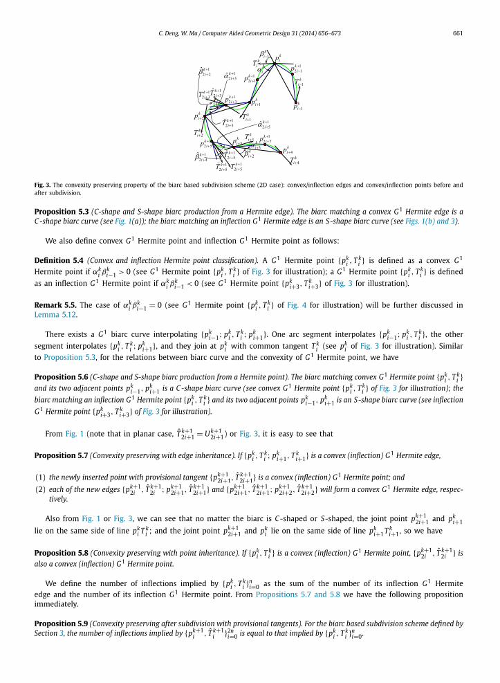
Fig. 3. The convexity preserving property of the biarc based subdivision scheme (2D case): convex/inflection edges and convex/inflection points before and after subdivision.
Proposition 5.3 (C-shape and S-shape biarc production from a Hermite edge). The biarc matching a convex G1 Hermite edge is a C-shape biarc curve (see Fig. 1(a)); the biarc matching an inflection G1 Hermite edge is an S-shape biarc curve (see Figs. 1(b) and 3).
We also define convex G1 Hermite point and inflection G1 Hermite point as follows:
Definition 5.4 (Convex and inflection Hermite point classification). A G1 Hermite point {pki , T
ki } is defined as a convex G1
Hermite point if αki β
ki−1 > 0 (see G1 Hermite point {pk
i , Tki } of Fig. 3 for illustration); a G1 Hermite point {pk
i , Tki } is defined
as an inflection G1 Hermite point if αki β
ki−1 < 0 (see G1 Hermite point {pk
i+3, Tki+3} of Fig. 3 for illustration).
Remark 5.5. The case of αki β
ki−1 = 0 (see G1 Hermite point {pk
i , Tki } of Fig. 4 for illustration) will be further discussed in
Lemma 5.12.
There exists a G1 biarc curve interpolating {pki−1; pk
i , Tki ; pk
i+1}. One arc segment interpolates {pki−1; pk
i , Tki }, the other
segment interpolates {pki , T
ki ; pk
i+1}, and they join at pki with common tangent T k
i (see pki of Fig. 3 for illustration). Similar
to Proposition 5.3, for the relations between biarc curve and the convexity of G1 Hermite point, we have
Proposition 5.6 (C-shape and S-shape biarc production from a Hermite point). The biarc matching convex G1 Hermite point {pki , T
ki }
and its two adjacent points pki−1, p
ki+1 is a C-shape biarc curve (see convex G1 Hermite point {pk
i , Tki } of Fig. 3 for illustration); the
biarc matching an inflection G1 Hermite point {pki , T
ki } and its two adjacent points pk
i−1, pki+1 is an S-shape biarc curve (see inflection
G1 Hermite point {pki+3, T
ki+3} of Fig. 3 for illustration).
From Fig. 1 (note that in planar case, T k+12i+1 = U k+1
2i+1) or Fig. 3, it is easy to see that
Proposition 5.7 (Convexity preserving with edge inheritance). If {pki , T
ki ; pk
i+1, Tki+1} is a convex (inflection) G1 Hermite edge,
(1) the newly inserted point with provisional tangent {pk+12i+1, T
k+12i+1} is a convex (inflection) G1 Hermite point; and
(2) each of the new edges {pk+12i , T k+1
2i ; pk+12i+1, T
k+12i+1} and {pk+1
2i+1, Tk+12i+1; pk+1
2i+2, Tk+12i+2} will form a convex G1 Hermite edge, respec-
tively.
Also from Fig. 1 or Fig. 3, we can see that no matter the biarc is C-shaped or S-shaped, the joint point pk+12i+1 and pk
i+1
lie on the same side of line pki T k
i ; and the joint point pk+12i+1 and pk
i lie on the same side of line pki+1 T k
i+1, so we have
Proposition 5.8 (Convexity preserving with point inheritance). If {pki , T
ki } is a convex (inflection) G1 Hermite point, {pk+1
2i , T k+12i } is
also a convex (inflection) G1 Hermite point.
We define the number of inflections implied by {pki , T
ki }n
i=0 as the sum of the number of its inflection G1 Hermite edge and the number of its inflection G1 Hermite point. From Propositions 5.7 and 5.8 we have the following proposition immediately.
Proposition 5.9 (Convexity preserving after subdivision with provisional tangents). For the biarc based subdivision scheme defined by Section 3, the number of inflections implied by {pk+1, T k+1}2n is equal to that implied by {pk, T k}n .
i i i=0 i i i=0
662 C. Deng, W. Ma / Computer Aided Geometric Design 31 (2014) 656–673
Fig. 4. Illustration of a G1 Hermite point with one degenerate angle being zero.
Now we have proved that after inserting the new points and defining the provisional tangent vectors, the number of inflections is not changed. In the following we focus on the issue that after computing the new tangent vectors the number of inflections is also not changed. To this aim, we first present three Lemmas for the signs of angles of inflection G1 Hermite point corresponding to the inflection G1 Hermite edge (Lemma 5.10), for the signs of angles of convex G1 Hermite points inherited from convex G1 Hermite points (Lemma 5.11) for the case of αk
i βki−1 = 0 (Lemma 5.12), respectively.
Lemma 5.10 (Convexity preserving with inflection edge-point inheritance). If {pki , T
ki ; pk
i+1, Tki+1} is an inflection G1 Hermite edge,
then {pk+12i+1, T
k+12i+1} is an inflection G1 Hermite point, and the signs of αk+1
2i+1, βk+12i are the same as those of αk+1
2i+1, βk+12i , respectively.
Proof. For an inflection G1 Hermite edge {pki , T
ki ; pk
i+1, Tki+1}, its corresponding new G1 Hermite point {pk+1
2i+1, Tk+12i+1} is an
inflection G1 Hermite point (see inflection G1 Hermite edge {pki+1, T
ki+1; pk
i+2, Tki+2} of Fig. 3 for illustration). Without loss
of generality, we can assume αki < 0, βk
i > 0 and |αki | > βk
i . Then
� T k2i+1 pk
2i+1 pki+1 = � pk+1
2i+1 pki+1 Ik
i+1 = � pki pk
i+1 Iki+1 + � pk+1
2i+1 pki+1 pk
i
= βki + � pk+1
2i+1 pki+1 pk
i > � pk+12i+1 pk
i+1 pki = � pk
i+1 pk+12i+1 T k+1
2i+1.
Then by Eq. (1),
T k+12i+1 = (1 − ω)T k+1
2i+1 + ωT k+12i+1
‖(1 − ω)T k+12i+1 + ωT k+1
2i+1‖,
and ω < 0.5 we have T k+12i+1 lies between pk
i+1 − pk+12i+1 and T k+1
2i+1. Thus we know that the signs of αk+12i+1, β
k+12i are the same
as those of αk+12i+1, β
k+12i . �
For convex G1 Hermite point {pki , T
ki }, a similar conclusion holds:
Lemma 5.11 (Convexity preserving with convex point-point inheritance). If {pk+1i , T k+1
i } is a convex G1 Hermite point with αk+1
i βk+1i−1 > 0, {pk+1
i , T k+1i } is also a convex G1 Hermite point, and the signs of αk+1
i , βk+1i−1 are the same as those of αk+1
i , βk+1i−1 ,
respectively.
Proof. From the condition αk+1i βk+1
i−1 > 0 and the definition of T k+1i , we have that both T k+1
i and T k+1i lie on the same
side of triangle pk+1i−1 , pk+1
i , pk+1i+1 , then T k+1
i = (1−ω)T k+1i +ωT k+1
i
‖(1−ω)T k+1i +ωT k+1
i ‖ also lies on the same side of triangle pk+1i−1 , pk+1
i , pk+1i+1 (see
convex G1 Hermite point pk+12i+5, T
k+12i+5 of Fig. 3 for illustration). So {pk+1
i , T k+1i } is also a convex G1 Hermite point, and the
signs of αk+1i , βk+1
i−1 are the same as those of αk+1i , βk+1
i−1 , respectively. �Lemma 5.12 (Convexity preserving under degenerate conditions). For G1 Hermite point {pk+1
i , T k+1i }, if αk+1
i βk+1i−1 = 0, then G1
Hermite point {pk+22i , T k+2
2i } is a convex G1 Hermite point (see Fig. 4).
Proof. Without loss of generality, we assume αk+1i = 0. Because there exists a G1 arc spline interpolating {pk+1
i , T k+1i }2n
i=0
and all consecutive points pki−1, pk
i , pki+1 are not collinear, we have then βk+1
i−1 �= 0.
By Lemma 5.10, for any newly inserted point pk+1i , αk+1
i βk+1i−1 > 0, then pk+1
i is a point with even index. Without loss of generality, we assume i = 2m and then pk+1
i = pk+12m = pk
m , T k+1i = T k
m . By Proposition 5.8 and Lemma 5.11, for a convex G1 Hermite point {pk
m, T km}, both {pk+1
2m−1, Tk+12m−1} and {pk+1
2m+1, Tk+12m+1} are convex G1 Hermite point, then we conclude that
{pkm, T k
m} is an inflection G1 Hermite point.Because every new G1 Hermite edge is convex G1 Hermite edge (see item (2) of Proposition 5.7), both {pk+1
i−1 , T k+1i−1 ;
pk+1, T k+1} and {pk, T k; pk , T k } are convex G1 Hermite edges. By Lemmas 5.10 and 5.11, no matter whether edges
i i i i i+1 i+1
C. Deng, W. Ma / Computer Aided Geometric Design 31 (2014) 656–673 663
{pkm−1, T
km−1; pk
m, T km} and {pk
m, T km; pk
m+1, Tkm+1} are convex or inflection G1 Hermite edges, the signs of αk+1
2m−1, βk+12m are
the same as those of αk+12m−1, βk+1
2m . That is, the signs of αk+1i−1 , βk+1
i are the same as those of αk+1i−1 , βk+1
i (see Fig. 4).
Because {pkm, T k
m} is an inflection G1 Hermite point, pkm−1, p
km+1 lie on opposite side of pk
m T km . Combining with the fact
that pkm−1, p
k+12m−1 lie on the same side of pk
m T km (see inflection G1 Hermite point {pk
i+3, Tki+3} of Fig. 3 for illustration). Then
pk+12m−1 = pk+1
i−1 , pk+12m+1 = pk+1
i+1 lie on the opposite side of pkm T k
m , i.e., pk+1i T k+1
i , too.
By the sign of αk+1i−1 is the same as that of αk+1
i−1 , we conclude that pk+22i−1, p
k+1i−1 lie on the same side of pk+1
i T k+1i (see
Fig. 4). By the sign of βk+1i is the same as that of βk+1
i , we conclude that pk+22i+1 and radial line pk+1
i T k+1i+1 lie on the same
side of pk+1i T k+1
i (see Fig. 4). Then pk+22i−1, p
k+22i+1 lie on the same side of pk+1
i T k+1i . Note that T k+2
2i = T k+1i , pk+2
2i−1, pk+22i+1 lie
on the same side of pk+1i T k+2
2i and T k+22i = (1−ω)T k+2
2i +ωT k+22i
‖(1−ω)T k+22i +ωT k+2
2i ‖ we conclude that {pk+22i , T k+2
2i } is a convex G1 Hermite point
(see Fig. 4). �Based on Lemmas 5.10, 5.11 and 5.12, we have
Proposition 5.13 (Convexity preserving after subdivision – from provisional tangents to final tangents). For the biarc based subdivision scheme defined by Section 3, the number of inflections implied by {pk+1
i , T k+1i }2n
i=0 is equal to that implied by {pk+1i , T k+1
i }2ni=0 .
Proof. Note that there exists a G1 arc spline Φk+1 interpolating {pk+1i , T k+1
i }, we have αk+1i �= 0 and βk+1
i �= 0. Because the order of computing the new tangents {T k+1
i } does not affect the convexity, we first replace {T k+1i } by {T k+1
i } of the convex G1 Hermite points and inflection G1 Hermite points whose indices are odds. From Lemmas 5.10 and 5.11 we conclude that if {pk+1
i , T k+1i } is convex G1 Hermite point with αk+1
i βk+1i−1 > 0, or is inflection G1 Hermite point with odd index, after
replacing T k+1i by T k+1
i , the convexity property of each G1 Hermite point and G1 Hermite edge does not change. Combining with item (2) of Proposition 5.7, all G1 Hermite edges are convex G1 Hermite edges.
In the following we consider the case of αk+1i βk+1
i−1 < 0 with even index, i.e., i = 2m.
In the case of αk+1i βk+1
i−1 < 0, pk+1i−1 and pk+1
i+1 lie in opposite side of pk+1i T k+1
i (see inflection G1 Hermite point {pk+1
2i+3, Tk+32i+3} of Fig. 3 for illustration). Because pk+1
i−1 and pk+1i+1 remain to lie on the same side of pk+1
i T k+1i , there are
three possibilities of T k+1i = (1−ω)T k+1
i +ωT k+1i
‖(1−ω)T k+1i +ωT k+1
i ‖ as follows:
(i) pk+1i−1 and pk+1
i+1 lie on opposite side of pk+1i T k+1
i .
In this case, the signs of angles αk+1i and βk+1
i−1 are the same as those of αk+1i and βk+1
i−1 , respectively. This means that after replacing T k+1
i by T k+1i , the convexity property of each G1 Hermite point and G1 Hermite edge is the same.
(ii) pk+1i−1 and pk+1
i+1 lie on the same side of pk+1i T k+1
i .
In this case, the sign of angle βk+1i−1 is different from that of βk+1
i−1 . {pk+1i , T k+1
i } then becomes a convex G1
convex point, and the convex G1 Hermite edge {pk+1i−1 , T k+1
i−1 ; pk+1i , T k+1
i } becomes an inflection G1 Hermite edge {pk+1
i−1 , T k+1i−1 ; pk+1
i , T k+1i }. So the number of inflections does not change.
(iii) One of pk+1i−1 and pk+1
i+1 lies on the line defined by pk+1i , T k+1
i .
Without loss of generality, we can assume that pk+1i+1 lies on the line defined by pk+1
i , T k+1i . So {pk+1
i , T k+1i ; pk+1
i+1 , T k+1i+1 }
is an inflection G1 Hermite edge and implies an inflection G1 Hermite point {pk+22i+1, T
k+22i+1} (see Fig. 4). By Lemma 5.12 we
know that {pk+22i , T k+2
2i } becomes a convex G1 Hermite point and then the number of inflections does not change.Combining all the above cases, we conclude that Proposition 5.13 holds. �From Propositions 5.9 and 5.13 we have
Theorem 5.14 (Convexity preserving for each level of subdivision in 2D). The biarc based subdivision scheme defined in Section 3 is convexity preserving for 2D curve interpolation.
5.2. Convexity preserving property of the 3D case
In this subsection, we assume that vectors T ki , T k
i+1 and pki+1 − pk
i are not coplanar and we adopt the same symbols used in Section 2.2.
The definition of convexity preserving in 3D is a very subtle issue because the position of an inflexion depends on the view direction if a curve has torsion. In our construction, the limit curve has local support and is G2 , then it must allow

664 C. Deng, W. Ma / Computer Aided Geometric Design 31 (2014) 656–673
Fig. 5. Convexity preserving under the projection of a 3D G1 Hermite edge to a plane: (a) a convex G1 Hermite edge {pki , T k
i ; pki+1, T k
i+1}; (b) an inflection G1 Hermite edge {pk
i , T ki ; pk
i+1, T ki+1}.
torsion. Since a 3D biarc can be constructed from a 2D biarc, we define a convex G1 Hermite edge, an inflection G1 Hermite edge, a convex G1 Hermite point and an inflection G1 Hermite point in 3D according to the respective cases of 2D . Though this definition seems to be arbitrary to some extent because it is based on the local osculating sphere, it is well-defined due to the fact that each 3D G1 Hermite data is always co-spherical, and if the proposed construction is applied, there exists one and only one 2D G1 Hermite data corresponding to it.
We define a convex G1 Hermite edge and an inflection G1 Hermite edge as follows:
Definition 5.15 (Convex and inflection edge classification). A G1 Hermite edge {pki , T
ki ; pk
i+1, Tki+1} is defined as a convex G1
Hermite edge if αki β
ki > 0 (see Fig. 2(a)); a G1 Hermite edge {pk
i , Tki ; pk
i+1, Tki+1} is defined as an inflection G1 Hermite edge
if αki β
ki ≤ 0 (see Fig. 2(b)).
Similarly, a convex G1 Hermite point and an inflection G1 Hermite point are defined as follows:
Definition 5.16 (Convex and inflection point classification). A G1 Hermite point {pki , T
ki } is defined as a convex G1 Hermite
point if αki β
ki−1 ≥ 0, a G1 Hermite point {pk
i , Tki } is defined as an inflection G1 Hermite point if αk
i βki−1 < 0.
For a G1 Hermite edge {pki , T
ki ; pk
i+1, Tki+1}, we have
Lemma 5.17 (Convexity preserving from 3D to arbitrary 2D plane projection). Let {pki , T
ki ; pk
i+1, Tki+1} be a convex (inflection) edge,
Π be a plane passing through pki pk
i+1 , U ki , U
ki+1 be the projections of T k
i , Tki+1 to Π , respectively, then {pk
i , Uki ; pk
i+1, Uki+1} is also a
convex (inflection) G1 Hermite edge.
Proof. Let qki , q
ki+1 be the intersections of lines qk
i Iki and qk
i+1 Iki+1 with Π respectively, then the projections of pk
i T ki and
pki+1T k
i+1 to Π will be pki qk
i and qki+1 pk
i+1, respectively (see Fig. 5).
In case of {pki , T
ki ; pk
i+1, Tki+1} being a convex G1 Hermite edge, vectors Ik
i − pki , pk
i+1 − Iki+1 lie on different side of pk
i pki+1
on Πki , so vectors qk
i − pki and pk
i+1 − qki+1 also lie on different side of pk
i pki+1 on Π (see Fig. 5(a)). Thus {pk
i , Uki ; pk
i+1, Uki+1}
is convex G1 Hermite edge. Similar conclusion also holds in case of {pki , T
ki ; pk
i+1, Tki+1} being an inflection G1 Hermite edge.
Lemma 5.17 thus holds. �We point out a simple lemma as follows:
Lemma 5.18. Let T ki = (1−ω)T k
i +ωT ki
‖(1−ω)T ki +ωT k
i ‖ , unit vectors T ki , ˜T k
i , ˜T k
i be the projections of T ki , T
ki , T k
i to a plane Π , then T ki = (1−ω)
˜T k
i +ω ˜T k
i
‖(1−ω)˜T k
i +ω ˜T k
i ‖.
The proof of this lemma is easy and we omit it here.By Lemma 5.17, the convexity property of G1 Hermite edge {pk
i , Tki ; pk
i+1, Tki+1} can be converted to the convexity of its
projection to plane passing through {pki , T
ki ; pk
i+1, Tki+1}. On the other hand, convexity property of G1 Hermite point {pk
i , Tki }
is defined on plane {pki−1, pk
i , pki+1}. Furthermore, by Lemma 5.18, the linear combination of 3D can also be converted to
that of the 2D case. Similar to the proof of the 2D case, we have
Proposition 5.19 (Convexity preserving after subdivision with provisional tangents). For the biarc based subdivision scheme defined by Section 3, the number of inflections implied by {pk+1
i , T k+1i }2n
i=0 is equal to that implied by {pki , T
ki }n
i=0 .
C. Deng, W. Ma / Computer Aided Geometric Design 31 (2014) 656–673 665
Proposition 5.20 (Convexity preserving after subdivision – from provisional tangents to final tangents). For the biarc based subdivision scheme defined by Section 3, the number of inflections implied by {pk+1
i , T k+1i }2n
i=0 is equal to that implied by {pk+1i , T k+1
i }2ni=0 .
We thus have
Theorem 5.21 (Convexity preserving for each level of subdivision in 3D). The biarc based subdivision scheme defined in Section 3 is convexity preserving for 3D curve interpolation.
6. Smoothness analysis
To make the text lighter, we assume that all angles in this section are positive if not stated explicitly. In case of some angles being negative, the proof is similar.
For convenience, we further summarize some notations as follows.
• αki : the angle from T k
i to pki pk
i+1; βki : the angle from pk
i pki+1 to T k
i+1; θk = maxi{αki , β
ki }.
• αki : the angle from T k
i to pki pk
i+1; βki : the angle from pk
i pki+1 to T k
i+1; θk = maxi{αki , β
ki }.
• αki : the angle from T k
i to pki pk
i+1; βki : the angle from pk
i pki+1 to T k
i+1; θk = maxi{αki , β
ki }.
• γ ki : the angle from T k
i to T ki , i.e. the angle from T k
i , T ki+1 to plane Πk
i .
It is easy to see that θk ≤ θk .We now prove that
Theorem 6.1. For the biarc based subdivision scheme defined in Section 3, limk→∞ θk = limk→∞ θk = 0.
The proof of this theorem requires some further discussions and we pose it in Appendix A.
Theorem 6.2. For the biarc based subdivision scheme defined in Section 3, the polygon series converges to a continuous curve.
Proof. Similar to the proof of Theorem 4.2 of Deng and Wang (2010), it is not difficult to show that the limit curve is continuous. �Theorem 6.3. For the biarc based subdivision scheme defined in Section 3, the limit curve is G1 continuous.
Proof. Following form Lemma A.4, Lemma A.6 we have
γ ki < ωθk < ω
(1 + 2ω
2
)k
θ0.
Then max{limk→∞ γ ki } = 0 and so for enough little neighborhood of a point, the control polygon can be seen as plane
polygon. Thus this theorem follows immediately from (A.16) and Theorem 6.2 of this article and Theorem 18 of Dyn and Hormann (2012). �7. Numerical examples and further discussions
In this section, we present several examples for smooth and convexity preserving interpolation by the biarc based subdi-vision scheme. To illustrate the quality of a subdivision curve, we also compute and plot the discrete curvatures of the curve after a finite number of subdivisions. For a point pk
i , its discrete curvature is determined by its discrete curvature circle, which pass through pk
i−1, pki , p
ki+1. The initial tangent vector T 0
i for p0i is the tangent vector at p0
i of the circle passing through p0
i−1, p0i and p0
i+1.We first explore the effect of free parameter ω (see Eq. (1)) to the limit curve in Example 1, in which nine limit curves are
generated by the biarc based subdivision scheme from a simple control polygon with free parameter ω as 0.05, 0.1, 0.15, 0.2, 0.25, 0.3, 0.35, 0.4, 0.45, respectively. The initial five points are (4.09, 5.21, 0), (3.79, 3.92, 1), (5.64, 2.48, 0), (7.98, 3.75, 0), (7.39, 5.69, 3). The limit curves as well as discrete curvature of each point are displayed in Fig. 6. To easily access the shape of these limit curves, we also display the discrete curvature plots for each of the limit curves (see Fig. 7). From the limit curves and their discrete curvature plots, we can see that for small ω such as 0.05, 0.1, 0.15, the limit curve have some visible jump points of curvature, though from the curvature plots we can see that the limit curves still seem to be curvature continuous. For big ω such as 0.35, 0.4, 0.45, the discrete curvatures of the limit curves seem to be jagged sometimes. From their discrete curvature plots, we can clearly see this effect. So though their limit curves seem to be curvature continuous, the limit curves are not fair. However for median ω such as 0.2, 0.25, 0.3, from the limit curves and their discrete curvature

666 C. Deng, W. Ma / Computer Aided Geometric Design 31 (2014) 656–673
Fig. 6. Illustration of limit curves of Example 1 with different blending ω.
plots, we can see that the limit curves seem to be curvature continuous and fair. So we recommend to set the free parameter ω be in the range of [0.2, 0.3]. In the following examples we let ω = 0.25.
To compare the effect of the biarc subdivision scheme with other schemes, a limit curve generated by the ternary four point subdivision scheme (Hassan et al., 2002), which generates C2 curves, and its discrete curvature plots are displayed in Fig. 8. From Fig. 8(b) we can see that though the limit curve of the ternary four point subdivision scheme is C2 continuous, the fact that the limit curve has many curvature extreme points implies that the limit curve is not fair. Two other examples (see Figs. 9, 10) also support this conclusion.
In the following examples, we show the convexity preserving and artifact removal effect of the biarc based subdivision scheme. A well-known deficiency of linear subdivision schemes is that their limit curves have big bump near a short

C. Deng, W. Ma / Computer Aided Geometric Design 31 (2014) 656–673 667
Fig. 7. Curvature plots of limit curves for Example 1: blue lines for ω = 0.05, 0.2, 0.35; red lines for ω = 0.1, 0.25, 0.4; and green lines for ω = 0.15, 0.3, 0.45. (For interpretation of the references to color in this figure legend, the reader is referred to the web version of this article.)
Fig. 8. The limit curve and its curvature plot of a ternary four point subdivision scheme: (a) the limit curve; (b) its curvature plot.
Fig. 9. Comparison of limit curves produced by the proposed subdivision scheme and another subdivision scheme: (a) limit curve produced by the proposed biarc based subdivision scheme; (b) limit curve produced by a ternary four point interpolatory subdivision scheme.
edge with adjacent very long edges (also see Fig. 10(a)). The biarc based subdivision scheme, however, produces very fair limit curves in such case (see Fig. 10(b)). The initial points for Example 2 are (2.5, 8.8, 0), (1.5, 8.0, 2), (3.0, 5.0, 0), (5.0, 5.0, 1), (6.5, 8.0, 0), (5.5, 8.8, 0), (4.0, 7.6, 0). The initial points for Example 3 are (4.7, 3.8, 0), (7.6, 3.8, 2), (7.7, 3.9, 2), (7.7, 5.3, −2), (4.7, 5.3, 0).
Finally, we give two more examples (see Figs. 11, 12) to show the property for generating spherical curves by the biarc based subdivision scheme. In these two examples, we first sample some initial data from source figures, then generate planar curves by the biarc based subdivision scheme, finally we map the planar initial data to spherical surface and generate

668 C. Deng, W. Ma / Computer Aided Geometric Design 31 (2014) 656–673
Fig. 10. A further comparison of limit curves produced by the proposed subdivision scheme and another subdivision scheme: (a) limit curve produced by the proposed biarc based subdivision scheme; (b) limit curve produced by a ternary four point interpolatory subdivision scheme.
Fig. 11. Designing an ocean star on a spherical surface by the proposed biarc based subdivision scheme: (a) planar case; (b) spherical case.
Fig. 12. Designing the head portrait of Mickey on a spherical surface by the proposed biarc based subdivision scheme: (a) planar case; (b) spherical case.

C. Deng, W. Ma / Computer Aided Geometric Design 31 (2014) 656–673 669
Fig. 13. Illustration for Lemma A.1.
spherical curves by the biarc based subdivision scheme. From the figures we can see that the limit curve are spherical curves if all the initial data are sampled from the spherical surface. These facts are consistent with Theorem 4.1.
From these examples and many other examples that we tested, we find that the limit curves produced by the proposed biarc based subdivision scheme is G2 continuous. It is however difficult to prove this conclusion at the moment. We thus pose a conjecture in this paper and leave the proof as future work.
Conjecture 1. For the biarc based subdivision scheme defined in Section 3, the limit curve is G2 continuous.
8. Conclusions and future work
We have described a biarc based subdivision scheme for 3D curve interpolation. It can be seen as an extension of the incenter subdivision scheme (Deng and Wang, 2010) to 3D for space curve subdivision. The scheme has some attractive properties, such as spherical curve generation, convexity preserving, artifacts removal and thus producing fair limit curves. How to prove that the limit curve is G2 continuous should however be further addressed as future work. The design of other higher order 3D interpolation curves by geometry driven subdivision schemes also deserves for future studies. Another attractive but difficult future work is to extend the proposed biarc based subdivision scheme for defining an interpolatory surface subdivision scheme that reproduces spherical surfaces.
Acknowledgements
This work is supported by NSFC (61003194, 61370166, 61379072), the Open Project Program of the State Key Lab of CAD&CG (Grant No. A1304), Zhejiang University, Research Grants Council of Hong Kong SAR (CityU 118512), and City Uni-versity of Hong Kong (Strategic Research Grant No. 7002735).
Appendix A. Proof of Theorem 6.1
The structure of this appendix is as follows. We first present two Lemmas of background knowledge. We then explore the angle relations after new tangent computation and angle relations after new point insertion. Finally, we get the final conclusions.
A.1. Two lemmas of background knowledge
Because T ki is defined as the linear combination of T k
i and T ki , first we give a lemma regarding the bounds of the angle
between one vector and its linear combination with another vector.
Lemma A.1. Assume that OT1 , OT2 be two unit vectors and
OT = (1 − ω)OT1 + ωOT2 (0 < ω < 0.5),
let the angle from OT2 to OT1 be α and the angle from OT to OT1 be β (see Fig. 13), we have then
β < ωα, (A.1)
Proof. By the definition of β , we have
cosβ = OT1 · OT
‖OT1‖ · ‖OT‖ = (1 − ω) + ω cosα√1 − 2(1 − ω)ω(1 − cosα)
.
It is easy to see that β, ωα < π2 , then
sinβ =√
1 − cos2 β =√
ω2 sin2 α
1 − 2(1 − ω)ω(1 − cosα)
<
√ω2 sin2 α
1 − 0.5(1 − cosα)= 2ω sin(0.5α). (A.2)

670 C. Deng, W. Ma / Computer Aided Geometric Design 31 (2014) 656–673
Fig. 14. Illustration for Lemma A.2.
Let f (α) = 2ω sin(0.5α) − sin(ωα), then
f ′(α) = 2ω cos(0.5α) · 0.5 − ω cos(ωα) = ω[cos(0.5α) − cos(ωα)
]< 0.
This means that f (α) < f (0) = 0 and then 2ω sin(0.5α) < sin(ωα). Combining with (A.2) we have β < ωα. �Lemma A.2. Let B be the projection of A to plane OBC (see Fig. 14). We have then
cos � AOC = cos � AOB cos � BOC. (A.3)
Proof. The proof of this lemma is easy and we omit it here. �A.2. Angle relations after new tangent computation
Because the new tangent for each point are computed as the linear blending of T ki and T k
i , in this subsection we bound angles {αk
i , βki } formed by new tangent {T k
i } and edge {pki pk
i+1}, angles γ ki formed by {T k
i } and plane {Πki } using angles
{αki , β
ki } formed by provisional tangents {T k
i } and edges {pki pk
i+1}.
Let pki−1 be a point on the line extended from pk
i−1 pki , then T k
i lies between pki pk
i−1 and pki pk
i+1 because it is sampled from the circle passing pk
i−1, pki and pk
i+1. From this simple fact we have
� T ki pk
i T ki ≤ max
{� pki−1 pk
i T ki , � pk
i+1 pki T k
i
} = max{αk
i , βki
} ≤ θk.
Noting that
T ki = (1 − ω)T k
i + ωT ki
‖(1 − ω)T ki + ωT k
i ‖ ,
by Lemma A.1 we have
� T ki pk
i T ki < ω � T k
i pki T k
i ≤ ωθk. (A.4)
Thus we can bound θk as
Lemma A.3. For the biarc based subdivision scheme defined in Section 3,
θk ≤ (1 + ω)θk. (A.5)
Proof. By the definitions of αki , α
ki and (A.4) we have
αki = � T k
i pki pk
i+1 ≤ � T ki pk
i T ki + � T k
i pki pk
i+1
≤ ωθk + αki ≤ (1 + ω)θk.
Similarly, we have βki < (1 + ω)θk , and thus θk < (1 + ω)θk . �
G1 Hermite data {pki , T
ki ; pk
i+1 T ki+1} are coplanar because there exists an arc segment Φk
i matching to the data. We denote this plane as Πk
i . By (A.4), the angle from T ki to pk
i T ki , a line in Πk
i , is less than ωθk . Because the angle between a line and a plane is the least angle among the angles formed by the line and other lines on the plane, we know that the angle between T k
i and Πki is less than ωθk . Similarly, the angle between T k
i+1 and Πki is also less than ωθk . Based on these facts, we bound
γ k as
i
C. Deng, W. Ma / Computer Aided Geometric Design 31 (2014) 656–673 671
Fig. 15. Illustration for Lemma A.4.
Fig. 16. Illustration for Lemma A.5.
Lemma A.4. For a convex G1 Hermite edge {pki , T
ki ; pk
i+1, Tki+1},
γ ki < ωθk. (A.6)
Proof. Let δki , η
ki be the angles between T k
i , −T ki+1 and Πk
i , respectively (see Fig. 15). Combining with (A.4) we have,
max{δk
i , ηki
} ≤ max{� T k
i pki T k
i , � (−T ki+1
)pk
i+1
(−T ki+1
)} ≤ ωθki .
Let U ki , −U k
i+1 be the projections of T ki , −T k
i+1 to plane Πki , respectively, by Proposition 5.20, the projection of a convex
G1 Hermite edge {pki , T
ki ; pk
i+1, Tki+1} to plane Πk
i , {pki , U
ki ; pk
i+1, Uki+1}, is also a convex G1 Hermite edge. Then U k
i , −U ki+1
lie on the same side of pki pk
i+1 (see Fig. 15), and so the projection of T ki − T k
i+1 to plane Πki lies also on the same side as U k
i .
Based on the scenario of pki T k
i , pki+1(−T k
i+1) lie on the same side or different side of Πki , we classify two cases to prove
this lemma.(1) pk
i T ki and pk
i (−T ki+1) lie on different side of Πk
i :
In this case, both Πki and Πk
i are between T ki and −T k
i+1, we have
γ ki = δk
i + ηki
2< ωθk.
(2) pki T k
i and pki (−T k
i+1) lie on the same side of Πki :
In this case, T ki , (−T k
i+1), Πki lie on the same side of Πk
i , then we have
γ ki < max
{δk
i , ηki
} ≤ ωθk.
Thus (A.6) holds. �Lemma A.5. For an inflection G1 Hermite edge {pk
i , Tki ; pk
i+1, Tki+1} (k > 0),
max{αk
i , βki
}< 2ωθk. (A.7)
Proof. Let U ki , U
ki+1 be the projections of T k
i , T ki+1 to plane Πk
i . Since {pki , T
ki ; pk
i+1, Tki+1} is an inflection G1 Hermite edge,
by Lemma 5.17, {pki , U
ki ; pk
i+1, Uki+1} is also an inflection G1 Hermite edge. Then one of {T k
i , U ki } and {T k
i+1, Uki+1} lies in
different side of pk pk . Without loss of generality, we assume that T k, U k lie in different side of pk pk (see Fig. 16).
i i+1 i i i i+1
672 C. Deng, W. Ma / Computer Aided Geometric Design 31 (2014) 656–673
Because T ki , U k
i lie in different side of pki pk
i+1, from Fig. 16 and Eq. (A.4), we have
αki = � T k
i pki pk
i+1 < � T ki pk
i T ki < ω � T k
i pki T k
i < ωθk. (A.8)
Let Mki be the projection of T k
i to plane Πki , by Lemma 5.18 and T k
i = (1−ω)T ki +ωT k
i
‖(1−ω)T ki +ωT k
i ‖ , we have
Uki = (1 − ω)T k
i + ωMki
‖(1 − ω)T ki + ωMk
i ‖.
Combining with Lemma A.1, we have
� T ki pk
i pki+1 ≤ � T k
i pki U k
i ≤ ω � T ki pk
i Mki ≤ ω � T k
i pki T k
i ≤ ωθki .
Let pki be a point on the extension line of pk
i+1 pki , from Fig. 16, we further have
βki = � pk
i pki+1T k
i+1 ≤ � pki pk
i+1 T ki+1 + ω � T k
i+1 pki+1 T k
i+1 < 2ωθk. (A.9)
From Eqs. (A.8) and (A.9), we conclude that this lemma holds. �A.3. Angle relations after point insertion
Lemma A.6. The sequence {θk} satisfies
θk+1 <1 + 2ω
2θk. (A.10)
Proof. According to {pki , T
ki ; pk
i+1, Tki+1} is convex or inflection G1 Hermite edge, we classify two cases to proof this lemma.
(1) {pki , T
ki ; pk
i+1, Tki+1} is a convex G1 Hermite edge.
Because T ki is the projection of T k
i to plane Πki , by Lemma A.2, we have
cosαki = cosγ k
i cosαki . (A.11)
Then
sin2 αki = 1 − cos2 γ k
i cos2 αki ≥ 1 − cos2 γ k
i = sin2 γ ki .
This means that sinαki ≥ sinγ k
i .
Because T k+12i is the projection of T k+1
2i to plane Πki (see Fig. 2), combining with the subdivision rules, we have
cos βk+12i = cosγ k
i cosαk
i
2.
Combining with cosαki = cosγ k
i cosαki , we have
cos2 βk+12i = cos2 γ k
i cos2 αki
2= cos2 γ k
i
1 + cosαki
2
= 1 − sin2 γ ki + cosγ k
i cosαki
2
≥ 1 − sinγ ki sinαk
i + cosγ ki cosαk
i
2
= 1 + cos(γ ki + αk
i )
2= cos2 γ k
i + αki
2.
Thus combining with Lemma A.4, we further have
βk+12i ≤ αk
i + γ ki
2≤ θk + γk
2<
1 + 2ω
2θk. (A.12)
Similarly,
αk+12i+1 <
1 + 2ωθk. (A.13)
2

C. Deng, W. Ma / Computer Aided Geometric Design 31 (2014) 656–673 673
(2) {pki , T
ki ; pk
i+1, Tki+1} is an inflection G1 Hermite edge.
From Fig. 2 and Lemma A.2, we can see that
cos αk+12i = cos � T k
i pki T k
i cos T ki pk
i pk+12i+1 > cos � T k
i pki T k
i cos � T ki pk
i pki+1
= cosγ ki cosαk
i = cosαki ,
then we have
αk+12i ≤ αk
i ≤ 2ωθki .
Similarly,
αk+12i+1 ≤ 2ωθk <
1 + 2ω
2θk. (A.14)
The lemma follows from these two cases immediately. �A.4. The final conclusions
By Lemma A.6 and induction we conclude that
θk <
(1 + 2ω
2
)k
θ0. (A.15)
By Lemma A.4, Eq. (A.15) and further induction, we conclude that
θk < (1 + ω)
(1 + 2ω
2
)k
θ0. (A.16)
References
Bézier, P.E., 1972. Numerical Control: Mathematics and Applications. John Wiley & Sons, New York.Bolton, K.M., 1975. Biarc curves. Comput. Aided Des. 7, 89–92.Costantini, P., Pelosi, F., 2001. Shape-preserving approximation by space curves. Numer. Algorithms 27, 237–264.Deng, C., Ma, W., 2012. Matching admissible G2 Hermite data by a biarc-based subdivision scheme. Comput. Aided Geom. Des. 29, 363–378.Deng, C., Wang, G., 2010. Incenter subdivision scheme for curve interpolation. Comput. Aided Geom. Des. 27, 48–59.Dyn, N., Hormann, K., 2012. Geometric conditions for tangent continuity of interpolatory planar subdivision curves. Comput. Aided Geom. Des. 29, 332–347.Dyn, N., Levin, D., Gregory, J.A., 1987. A 4-point interpolatory subdivision scheme for curve design. Comput. Aided Geom. Des. 4, 257–268.Dyn, N., Levin, D., Liu, D., 1992. Interpolatory convexity-preserving subdivision schemes for curves and surfaces. Comput. Aided Des. 24, 211–216.Goodman, T.N.T., Ong, B.H., 1997. Shape preserving interpolation by space curves. Comput. Aided Geom. Des. 15, 1–17.Hassan, M.F., Ivrissimitzis, I.P., Dodgson, N.A., Sabin, M.A., 2002. An interpolating 4-point C2 ternary stationary subdivision scheme. Comput. Aided Geom.
Des. 19, 1–18.Hoschek, J., 1992. Circular splines. Comput. Aided Des. 11, 611–618.Kaklis, P.D., Karavelas, M.I., 1997. Shape-preserving interpolation in R3. IMA J. Numer. Anal. 17, 373–419.Marinov, M., Dyn, N., Levin, D., 2005. Geometrically controlled 4-point interpolatory schemes. In: Dodgson, N.A., Floater, M.S., Sabin, M.A. (Eds.), Advances
in Multiresolution for Geometric Modeling. Springer-Verlag.Piegl, L.A., Rajab, K., Smarodzinava, V., Valavanis, K.P., 2009. Using a biarc filter to compute curvature extremes of NURBS curves. Eng. Comput. 25, 379–387.Sabin, M.A., 1977. The use of piecewice forms for the numerical representation of shape. Report No. 60. Computer and Automation Institute, Hungarian
Academy of Science, Budapest.Sabin, M.A., Dodgson, N., 2005. A circle-preserving variant of the four-point subdivision scheme. In: Dæhlen, M., Morken, K., Schumaker, L.L. (Eds.), Mathe-
matical Methods for Curves and Surfaces. Tromso Conference. Nashboro Press.Sandel, G., 1937. Geometry of compound curve. Z. Angew. Math. Mech. 17, 301–302.Sharrock, T.J., 1987. Biarcs in three dimensions. In: Proceedings on Mathematics of Surfaces II. Cardiff, United Kingdom, pp. 395–411.Yang, X., 2006. Normal based subdivision scheme for curve design. Comput. Aided Geom. Des. 23, 243–260.