a better heuristic for orthogonal graph drawings

C o m p u t a t i o n a l

G e o m e t r y Theory and Applications

ELSEVIER Computational Geometry 9 (1998) 159-180

A better heuristic for orthogonal graph drawings

Therese Biedl a,*, Goos Kant b,1

a RUTCOR - Rutgers University, P.O. Box 5062, New Brunswick, NJ 08903-5062, USA b Department of Computer Science, Utrecht University, Padualaan 14, 3584 CH Utrecht, The Netherlands

Communicated by R. Tamassia; submitted 9 March 1995; revised August 1996 and January 1997; accepted 7 August 1997

Abstract

An orthogonal drawing of a graph is an embedding in the plane such that all edges are drawn as sequences of horizontal and vertical segments. Linear time and space algorithms for drawing biconnected planar graphs orthogonally with at most 2n + 4 bends on a grid of size n x n are known in the literature.

In this paper we generalize this result to connected and non-planar graphs. Moreover, we show that in almost all cases each edge is bent at most twice. The algorithm handles both planar and non-planar graphs at the same time. © 1998 Elsevier Science B.V.

1. In troduct ion

The research area of graph drawing has become an extensively studied field which presents an exciting connection between computational geometry and graph theory. The wide spectrum of applications includes VLSI-layout, software engineering, and project management (see [6] for an up-to-date overview with more than 300 references). The aesthetic quality of a drawing cannot be precisely defined, and depending on the application different criteria have been used. Some important charac- teristics of a "readable" representation are the number of bends, the number of crossings, the sizes of the angles, and the required area.

In this paper we study the problem of orthogonal drawings, i.e., the drawing of a graph G = (V, E) where vertices are drawn as points and each edge is represented by a sequence of alternating horizontal and vertical segments. Such a representation is possible only when every vertex has at most four incident edges. Unless otherwise specified, we assume from now on that all graphs satisfy this condition. Then any graph G has an orthogonal drawing. In [ 11,16] it was shown that deciding whether G can be embedded in a grid of prescribed area is NP-complete. Sch~iffter showed that any graph can be

~ An extended abstract of this paper was presented at the 2nd Annual European Symp. on Algorithms, Utrecht, 1994. * Corresponding author. E-maih [email protected]. Research was supported by the ESPRIT Basic Research Actions program of the EC under contract No. 7141 (project

ALCOM II) and the ESPRIT Long Term Research Project 20244 (project ALCOM-IT). E-marl: [email protected].

0925-7721/98/$19.00 © 1998 Elsevier Science B.V. All rights reserved. PII S0925-7721 (97)00026-6

160 T. Biedl, G. Kant / Computational Geometry 9 (1998) 159-180

embedded in a 2n x 2n-grid with at most two bends per edge [22]. For graphs with maximum degree 3, a very recent paper showed that they can be embedded in an rn/2~ x In/2] -grid with In/21 +2 bends [3].

If G is planar, it can be embedded in an n x n grid with 2n + 4 bends if it is biconnected, and 2.4n + 2 bends otherwise [23,25]. The number of bends along each edge is at most 4. For triconnected planar graphs better bounds are known [2,15]. Independently of this work, Liu et al. [19] presented a linear-time algorithm for drawing biconnected planar graphs with at most 2 bends per edge (except the octahedron) and at most 2n + 4 bends in total on a grid of size at most (n + 1) x (n + 1).

If a combinatorial embedding of a planar graph is given, an orthogonal representation of it with minimal number of bends can be computed in O(n 2 log n) time [24]. The time complexity can be reduced to O(nlv5 lox/l-0~) time using the recent work by Garg and Tamassia [14]. However, there is no non-trivial upper bound on the number of bends in an edge. If the embedding is not given, the problem becomes NP-hard [ 13]. In particular, it is even NP-hard to approximate the minimum number of bends in a planar orthogonal drawing with a n O(n l-e) error for any E > 0 [13].

The latter motivates the research for a quick and very general heuristic to construct orthogonal representations of planar and non-planar graphs. In this paper we present a new algorithm that runs in O(n) time and produces orthogonal drawings of connected planar and non-planar graphs with the following properties: (i) the total number of bends is at most 2n ÷ 2; (ii) the number of bends along each edge is at most 2 (unless the graph is the octahedron and we want a planar drawing); (iii) the area of the embedding is n x n. For planar biconnected graphs, linear time algorithms were already known, yielding an area of at most n x n and at most 2n + 4 bends [23]. Hence our contribution is the fact that every edge is bent at most twice, and the generalization to non-biconnected and non-planar graphs. The result is obtained by constructing orthogonal drawings of the blocks using the so-called st-ordering and merging all these drawings into one orthogonal drawing of the entire graph.

The paper is organized as follows. Section 2 gives some definitions and introduces the st-ordering. In Section 3 the algorithm for biconnected graphs is explained. It is extended to non-biconnected graphs in Section 4. In Section 5 we explain how to arrive at a linear time implementation. In Section 6 we give remarks regarding issues that are vital for implementing the algorithm. Section 7 contains remarks and open problems. We provide three appendices, where we show how to compute a special planar embedding and st-ordering, how to improve the algorithm a little for simple graphs, and where we give a detailed example for a 1-connected graph.

2. Definitions

Let G = (V, E) be a graph, n = IVI, m = [El. For most of the paper, we consider only 4-graphs, i.e., graphs of maximum degree 4. Here m = 1 }-~v~v deg(v) ~< 2n. Call such a graph 4-regular if all vertices have exactly 4 neighbors. An orthogonal drawing of G is an embedding of G in the plane such that all edges are drawn as sequences of horizontal and vertical segments. A point where the drawing of an edge changes its direction is called a bend of this edge. If the drawing of an edge has at most k bends, we call this edge k-bent. We assume that all vertices and bends are drawn on integer points. If the drawing can be enclosed by a box of width nl and height n2, we call it an embedding with gridsize nl x n 2 and area nl • n2.

Unless otherwise specified, we consider only connected graphs, and we assume that the graph is simple, i.e., has neither loops nor multiple edges. A vertex v is called a cutvertex if removing v and

T. Biedl, G. Kant/Computational Geometry 9 (1998) 159-180 161

i i l ill . . . .

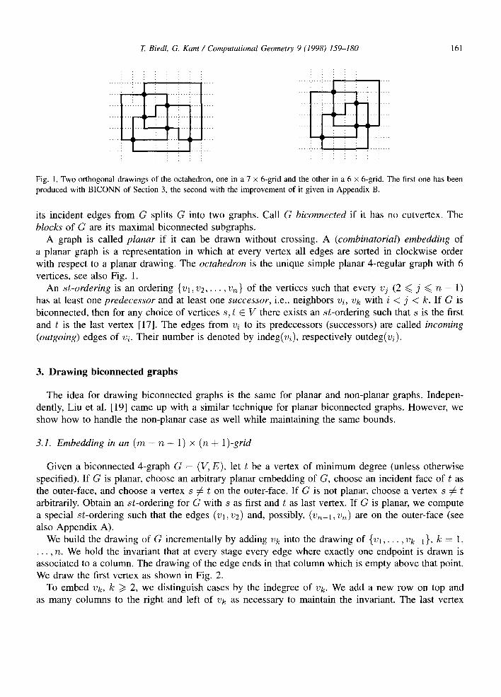
Fig. 1. Two orthogonal drawings of the octahedron, one in a 7 x 6-grid and the other in a 6 x 6-grid. The first one has been produced with BICONN of Section 3, the second with the improvement of it given in Appendix B.

its incident edges from G splits G into two graphs. Call G biconnected if it has no cutvertex. The blocks of G are its maximal biconnected subgraphs.

A graph is called planar if it can be drawn without crossing. A (combinatorial) embedding of a planar graph is a representation in which at every vertex all edges are sorted in clockwise order with respect to a planar drawing. The octahedron is the unique simple planar 4-regular graph with 6 vertices, see also Fig. 1.

An st-ordering is an ordering { V l , V 2 , . . - , Vn} of the vertices such that every vj (2 ~< j ~< n - 1) has at least one predecessor and at least one successor, i.e., neighbors vi, vk with i < j < k. If G is biconnected, then for any choice of vertices s, t E V there exists an st-ordering such that s is the first and t is the last vertex [17]. The edges from vi to its predecessors (successors) are called incoming (outgoing) edges of vi. Their number is denoted by indeg(vi), respectively outdeg(vi).

3. Drawing biconnected graphs

The idea for drawing biconnected graphs is the same for planar and non-planar graphs. Indepen- dently, Liu et al. [19] came up with a similar technique for planar biconnected graphs. However, we show how to handle the non-planar case as well while maintaining the same bounds.

3.1. Embedding in an (m - n + 1) x (n + 1)-grid

Given a biconnected 4-graph G = (V, E), let t be a vertex of minimum degree (unless otherwise specified). If G is planar, choose an arbitrary planar embedding of G, choose an incident face of t as the outer-face, and choose a vertex s ¢ t on the outer-face. If G is not planar, choose a vertex s ¢ t arbitrarily. Obtain an st-ordering for G with s as first and t as last vertex. If G is planar, we compute a special st-ordering such that the edges (vl, v2) and, possibly, (vn-1, vn) are on the outer-face (see also Appendix A).

We build the drawing of G incrementally by adding vk into the drawing of { v l , . . . , vk-1}, k = 1, . . . , n. We hold the invariant that at every stage every edge where exactly one endpoint is drawn is associated to a column. The drawing of the edge ends in that column which is empty above that point. We draw the first vertex as shown in Fig. 2.

To embed vk, k ~> 2, we distinguish cases by the indegree of vk. We add a new row on top and as many columns to the right and left of vk as necessary to maintain the invariant. The last vertex


l l I l l I I I I I

i l i i i

I l i a I I I I l l l l

Fig. 2. Embedding of the first vertex for various degrees.

I O l O I I l I I I l I

l l e l I e

Fig. 3. Embedding of vk, k ~> 2, for indeg(vk) = 1,2, 3, 4.

might have four predecessors, in which case we add two rows to accommodate it. The procedure is demonstrated for a vertex of degree 4 in Fig. 3. For a vertex of smaller degree, we use less columns.

Each outgoing edge of vk is assigned to one of the columns. This assignment is made according to the planar embedding for planar graphs. For non-planar graphs, any assignment is feasible.

We refer to this algorithm as BICONN. We estimate the obtained grid-size and number of bends in the following. Define the characteristic funct ion X(') to be 1 whenever what is inside the parenthesis is true, and 0 otherwise.

L e m m a 3.1. The width is m - n + 1, the height is at most n + x(deg(vn) = 4).

Proof. As one checks easily case by case, we increase the number of columns by outdeg(vi) - 1 for i ¢ 1, n. vl uses outdeg(vl) new columns, v~ uses no new column, and outdeg(v~) = 0. So the number of columns is

outdeg(vi) + ou tdeg (v~)+ ~ ( o u t d e g ( v ) - 1) = Z ( o u t d e g ( v ) - 1) + 2 = m - n + 2. vT~vl ,vn vEV

Every vertex ~ v~ increases the number of rows by 1. Vertex vn needs two rows if it has degree 4, and one row otherwise. So the number of rows is n + x(deg(vi ) = 4) + x(deg(v~) = 4). The proof now is finished since the width (height) is one less than the number of used columns (rows). []

L e m m a 3.2. There are at most 2m - 2n + 3 + x(deg(vn) -- 4) bends.

Proof. Case by case one checks that there are indeg(vi) - 1 and outdeg(vi) - 1, hence deg(vi) - 2 new bends for i ¢ 1, n. Embedding Vl gives at most deg(v]) bends. Embedding vn gives deg(vn) bends if deg(v~) = 4 and deg(v~) - 1 bends otherwise. Hence the number of bends is at most

Z (deg(v) - 2) + 3 + x(deg(v~) = 4) = 2m - 2n + 3 + x(deg(v~) = 4). [] vEV

L e m m a 3.3. All but at most two edges are 2-bent. The two exceptions are the edge at the bottom connection o f Vl, which exists only i f deg(vl) = 4; and the edge at the top connection o f vn, which

exists only i f deg(vn) = 4.

T. Biedl, G. Kant / Computational Geometry 9 (1998) 159-180 163

¢ ¢ ¢ ¢ ¢ ,

! ¢ ¢ ¢ ¢ ! O e O e o o

Fig. 4. We use the bottom connection at v~ for the edge (vl, 132) and can save one row. We use the edge (v,~-t, vn) for the top-connection at v,~, and introduce a crossing if necessary. Then all edges have at most 2 bends.

Proof. Assume we have an edge e = (vi, vj) with i < j . We consider the number of bends at e when embedding either endpoint. If outdeg(vi) ~< 3, then e gets at most one bend at vi. If indeg(vj) ~< 3, then e gets at most one bend at vj. So the only way e could have more than two bends is that either outdeg(vi) -- 4 or indeg(vj) -- 4.

This can happen only if i = 1 and deg(vl) = 4; or if j -- n and deg(v~) = 4. Moreover, it can happen only to the edge at the bottom connection of vl, since only this edge gets two bends at vl; or to the edge at the top connection Vn, since only this edge gets two bends at vn. []

Lemma 3.4. All edges can be made 2-bent for non-planar drawings.

Proof. Since we have an st-ordering, there must be edges (vl,/32) and (vn-1, v~). Assume deg(vl) = 4. Since we have a non-planar drawing, we have the freedom to assign the edge (vl, v2) to the connection at the bottom of v~. Thus, this edge has only two bends. As seen in Fig. 4, this assignment also enables us to place vl and v2 in one row and save one row.

Assume deg(v~) = 4. If the left-most or right-most column of the incoming edges belongs to the edge (Vn-l, vn), then we can make this edge use the top connection of vn, and thus the edge gets only two bends. Otherwise, we slightly change the drawing of vn and introduce a crossing, so that the edge gets only two bends. See Fig. 4 for an illustration. []

Lemma 3.5. All edges can be made 2-bent for planar drawings, unless the graph is the octahedron.

Proof. We apply exactly the same technique as in the previous proof. However, since we have no choice in the assignment of columns, we have to make sure that the edge (vl, v2) is on the outer-face of the planar embedding. Also, since we may not introduce a crossing, we have to make sure that the edge (Vn-l, vn) is on the outer-face. Such an st-ordering exists (after a possible change of the planar embedding) for all graphs except the octahedron (see Appendix A). []

Lemma 3.6. For a planar graph, BICONN gives a planar orthogonal drawing that exactly reflects the planar embedding which we had after computation of the st-ordering.

Proof. Obviously there is no crossing after embedding v I and v2. We will show that we produce no crossing when adding Vi+l, i > 1. Let G(i) be the subgraph induced by V l , . . . , vi, embedded as induced by G. Let E(i) be the set of edges from G(i) to G - G(i). For an edge in E(i) the endpoint in G(i) must be on the outer-face of G(i), otherwise we had a crossing. At least two edges of E(i) must be on the outer-face of G, by biconnectivity. In fact, exactly two edges of E(i) are on the outer-face, otherwise we did not have an st-ordering. Let E(i) be sorted in clockwise order, starting and ending with the two edges on the outer-face of G.


Let L(i) be the list of columns that contain an unfinished edge, at the time before embedding vi+l. Let them be sorted from left to right. The crucial observation is that E(i) and L(i) are in correspondence, i.e., the j th element in E(i) ends in the j th element of L(i). We show this by induction on i.

The claim is true for Vl, since we assigned columns according to the planar embedding. Assume it was true after step i. By planarity the incoming edges of Vi+l are consecutive in E(i). If there were another edge between them, then it would not be on the outer-face of G(i + 1), a contradiction. Since E(i) and L(i) are in correspondence, the columns of the incoming edges of vi are in consecutive order in L(i), and we do not cross any other edge when embedding vi+l.

For any st-ordering the incoming (outgoing) edges of a vertex v are consecutive in the rotation around v [25]. Since we assigned columns according to the planar embedding, after embedding vi+l we have the correspondence between E(i + 1) and L(i ÷ 1). With that we also have shown that the drawing exactly reflects the planar embedding. []

3.2. Embedding in an n × n-grid

It is possible to save a little bit in grid-size and bends for simple graphs. It might seem tedious to spend extra effort in order to reduce the width by just one unit. However, this is extremely useful when embedding non-biconnected graphs. Here each block is embedded separately, so in all we achieve a reduction in width equal to the number of blocks.

The crucial idea is that it is possible to find a vertex v* which can be embedded in the row of one of its neighbors. Finding v* needs a lengthy case analysis, which we defer to Appendix A. For now, it suffices to know that v* is chosen after we had an st-ordering and a planar embedding, and the choice of it does not change either of them.

Lemma 3.7. Assume G is a simple. There exists a vertex v* ~ vl , Vn, and an improvement of BICONN, such that the width is m - n + x(deg(v*) : 2), the height is n - 1 ÷ x(deg(vn) : 4), and the number of bends is 2m - 2n ÷ 1 + x(deg(v*) : 2) + x(deg(vn) : 4).

Proof. See Appendix A. []

With this improvement, we get the following lemma for simple graphs.

L e m m a 3.8. For simple graphs, the width and height is n - 1 + x ( G 4-regular), and the number of bends is m + 2. x (G 4-regular).

Proof. Apply BICONN and the improvement. We distinguish cases by the number of edges. Assume m ~< 2 n - 2 . Then, by the choice o fvn as a vertex of minimum degree, we have deg(vn) ~< 3. Therefore, we get at most an (m - n + 1) × (n - 1)-grid and 2m - 2n + 2 bends. Applying m ~< 2n - 2, we arrive at the results.

Assume m ~> 2n - 1. Then, by the choice of vn as a vertex of minimum degree, we have deg(v) ~> 3 for all v ~ vn. Since v* ~ v~, we have deg(v*) ~> 3, and we get an ( m - n ) × ( n - 1 +x(deg(vn) = 4))- grid and 2m - 2n + 1 + x(deg(vn) = 4) bends. If ra = 2n - 1, then deg(vn) ~< 3, and the bounds follow. If m :- 2n, then G is 4-regular, and the bounds follow as well. []


We reformulate the worst case of Lemma 3.8, and combine it with the results of the previous section, to give the main theorem for biconnected graphs.

Theorem 1. Let G be a biconnected simple 4-graph with n vertices. Then G can be embedded in an n x n-grid with at most 2n ÷ 2 bends. I f G is planar, then so is the drawing. Every edge is 2-bent, unless G is the octahedron and we want a planar drawing.

4. Connected graphs

In this section we describe how to embed simple graphs which are not biconnected with bounds similar to those in Theorem 1. To do so we split the graph into its blocks and embed them separately.

We need to draw parts of the graph in a special way. To describe it, we need two definitions. We say that a vertex v is drawn as f inal vertex if v and deg(v) - 1 of its incident edges are drawn in the last row. This in particular implies that deg(v) <~ 3. We say that a vertex w is drawn with right angle if deg(w) = 2, and the two incident edges form a fight angle. Using BICONN, we can draw every biconnected graph such that one vertex is drawn as final vertex, and any number of vertices is drawn with fight angle.

L e m m a 4.1. Let G be a simple biconnected 4-graph. Let v with deg(v) ~< 3 be given (and on the outer-face in the planar case). Let w ] , . . . , ws be vertices in V - {v} with deg(wj) -- 2, j = 1 , . . . , s.

G can be drawn with v as f inal vertex in an (n - 1) x (n - 1)-grid with m bends. Every edge is 2-bent. Every wj, j = 1 , . . . , s, is drawn with right angle.

Proof. Choose an st-ordering with v as last vertex, and produce a drawing F of G using BICONN and the improvement. This draws v as final vertex. Every edge is 2-bent since G is not 4-regular and therefore not the octahedron.

Now for each w j, j = 1 , . . . , s, check whether it is drawn with right angle. If it is not, check whether any incident edge of wj has a bend. If so, move wj to this bend. Otherwise, by the construction of BICONN and the improvement, we know that wj is drawn using the top and bottom connection. Cut the drawing at the column of wj, and add a new column, as shown in Fig. 5. Place wj at one of the resulting right angles. Since both incident edges of wj had no bend before, all edges in the resulting drawing have at most 2 bends.

So in order to achieve a right angle at wj, we at the worst add a column and one bend. We have m ~< 2n - 1 - s, since deg(v) ~< 3, and deg(wj) = 2 and wj ~ v for j = 1 , . . . , s. Roughly speaking, this reduction in the number of edges makes up for the added columns and bends. To precisely analyze the obtained size, we distinguish cases depending on v*, the vertex crucial for the improvement step.

Fig. 5. If wj is not drawn with a right angle, we can achieve this by cutting the drawing, and adding a column and a bend.

166 T. Biedl, G. Kant/Computational Geometry 9 (1998) 159-180

If deg(v*) = 3, then the drawing F was in an (m - n) × (n - 1)-grid and had 2 m - 2n + 1 bends. So the final width is at most m - n + s ~< n - 1, and the final number of bends is at most 2m - 2n + 1 + s ~< m. If deg(v*) = 2, then v* was drawn with right angle (see Appendix A). So if v* E { w l , . . . , w~}, then we had to add at most s - 1 columns and bends. So the final width is at most m - n + l + s - 1 < ~ n - l , and the final number of bends is at most 2 m - 2n + 2 + s - 1 ~<m. If deg(v*) = 2, but v* gg { W l , . . . , w~}, then in fact m ~< 2n - 2 - s, since v* ~ v~ = v. The final width is at most m - n + 1 + s ~< n - 1, and the final number of bends is at most 2m - 2n + 2 + s ~< m. []

The following two lemmas show how by merging such drawings we can get a drawing of the full graph of similar size. We distinguish by whether the graph has an edge whose removal disconnects the graph (such an edge is called a bridge). Also, we first treat graphs that have at least one vertex with degree less than four.

L e m m a 4.2. Let G be a simple 4-graph without bridges. Let v with deg(v) ~< 3 be given (and on the outer-face in the planar case). G can be drawn with v as final vertex in an (n - 1) x (n - 1)-grid with m bends. Every edge is 2-bent.

Proof . We proceed by induction on the number of cutvertices. In the base case G is biconnected and we apply Lemma 4.1.

For the induction step note first that v cannot be a cutvertex (otherwise by deg(v) ~< 3 it would be contained in a bridge). Let Go be the unique block containing v. Let V l , . . . , vs be the cutvertices of G in Go. Let Gi be the subgraph of G consisting of vi and the connected components of G - vi not containing Go. Denote by ni, respectively mi, the number of vertices and edges of Gi (i = 0 , . . . , s).

8 There is no edge in common between any of the G~ s, so Y~'~i=0 mi = m. Also, the intersection of the vertices of Go and Gi (1 ~< i <~ s) is vi, and the intersection of the vertices of Gi and Gj is empty if i ¢ j . Hence ~ = n E i = 0 / ~ i ÷ 8.

Since G has no bridge, vi is not a cutvertex for Gi, so Gi has fewer cutvertices than G. If G was planar and we take as embedding of Gi the one that is induced by G then (since v was on the outer-face of G) also vi is on the outer-face of Gi. So by induction Gi can be embedded in an (h i -- 1) × (ni - 1)-grid with mi bends and vi as final vertex.

Embed Go as described in Lemma 4.1, and draw v as final vertex and v l , . . . , v~ with right angle. For each Gi, consider the placement of vi in the drawing of Go, and assume it was drawn using the

I

I

. : _ 7 _

vi

Fig. 6. We add rows and columns next to the drawing of v~ in Go, and place Gi in them.


fight and the top connection. Assume that vi is drawn in Gi using the bottom and left connection (we can achieve this by rotating Gi). Add ni - 1 rows below the row of vi and add ni - 1 columns left and right to the column of vi. Merge Gi into these added rows and columns. See also Fig. 6.

The width of the drawing of Go was no - 1. For each Gi, we added ni - 1 columns. The drawing of Gi fits into these columns, since the width of it was ni - 1, and since we can reuse the column of vi for G~. Therefore, the total width is }-~=0(ni - 1) = n - 1. The estimation for the height is the same. Each of the Gi was drawn with mi bends. No bends were added when merging the graphs, so the total number of bends is ~-~'~i~0 mi = m. In each drawing of a subgraph, all bends had at most two bends, so the same holds for the final drawing. []

L e m m a 4.3. Let G be a simple 4-graph. Let v with deg(v) ~< 3 be given (and on the outer-face in the planar case). G can be drawn with v as f inal vertex in an (n - 1) x (n - 1)-grid with m bends.

Every edge is 2-bent.

Proof. We proceed by induction on the number of bridges. We are done if there are none, by the above lemma. So assume G has a bridge (vl, v2). Removing it splits G into two graphs Gl and G2 (we assume that vi E GO. Denote by ni and mi the number of their vertices and edges. Then nl + n2 = n and m l + m 2 = m - 1.

Assume G1 contains v (the vertex to be drawn as final vertex). Both G1 and G2 have at least one bridge less. By induction, embed GI with v as final vertex, and G2 with v2 as final vertex. In the resulting drawing of G1, Vl has a connection in one direction free, assume it is to the left. Add n2 columns to the left of Vl and n2 rows below it. Place the drawing of G2 in the space, and connect Vl and v2 with one bend. The resulting grid has width and height/z 1 - - 1 ÷ n 2 = n - - 1 and ml + m 2 + 1 = m bends. See also Fig. 7. []

In fact, by rotating the drawing of G2 and using a more general definition of "final vertex", one can avoid the bend in the edge (vl, v2) and achieve only m - br bends for a graph with br bridges.

So, if G is not 4-regular, then choose any vertex of degree ~< 3 to be v, and embed G as described in the proofs of the previous lemmas. If G is 4-regular, then it cannot have a bridge (otherwise removing the bridge would give a subgraph with exactly one vertex of odd degree, a contradiction). Split G at a cutvertex v to obtain G1 and G2. If G was planar, this also involves changing the embedding such that

! : ! i

Fig. 7. How to merge a subgraph connected by a bridge.


V l

G2

I

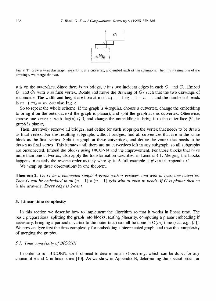
Fig. 8. To draw a 4-regular graph, we split it at a cutvertex, and embed each of the subgraphs. Then, by rotating one of the drawings, we merge the two.

v is on the outer-face. Since there is no bridge, v has two incident edges in each G1 and G2. Embed G1 and G2 with v as final vertex. Rotate and move the drawing of G2 such that the two drawings of v coincide. The width and height are then at most nl - 1 + n2 - 1 = n - 1 and the number of bends is rrq + m2 = m. See also Fig. 8.

So to repeat the whole scheme: If the graph is 4-regular, choose a cutvertex, change the embedding to bring it on the outer-face (if the graph is planar), and split the graph at this cutvertex. Otherwise, choose one vertex v with deg(v) ~< 3, and change the embedding to bring it to the outer-face (if the graph is planar).

Then, iteratively remove all bridges, and define for each subgraph the vertex that needs to be drawn as final vertex. For the resulting subgraphs without bridges, find all cutvertices that are in the same block as the final vertex. Split the graph at these cutvertices, and define the vertex that needs to be drawn as final vertex. This iterates until there are no cutvertices left in any subgraph, so all subgraphs are biconnected. Embed the blocks using BICONN and the improvement. For those blocks that have more than one cutvertex, also apply the transformation described in Lemma 4.1. Merging the blocks happens in exactly the reverse order as they were split. A full example is given in Appendix C.

We wrap up these observations in one theorem.

Theorem 2. Let G be a connected simple 4-graph with n vertices, and with at least one cutvertex. Then G can be embedded in an (n - 1) x (n - 1)-grid with at most m bends. I f G is planar then so is the drawing. Every edge is 2-bent.

5. Linear time complexity

In this section we describe how to implement the algorithm so that it works in linear time. The basic preparations (splitting the graph into blocks, testing planarity, computing a planar embedding if necessary, bringing a particular vertex to the outer-face) can all be done in O(m) time (see, e.g., [5]). We now analyze first the time complexity for embedding a biconnected graph, and then the complexity of merging the graphs.

5.1. Time complexity o f B ICONN

In order to run BICONN, we first need to determine an st-ordering, which can be done, for any choice of s and t, in linear time [10]. As we show in Appendix B, determining the special order for

T. Biedl, G. Kant / Computational Geomet~" 9 (1998) 159-180 169

planar graphs can also be done in linear time. So we only need to worry about the time needed for embedding one vertex.

Since we add new rows always on top of the previous drawing, the y-coordinate of a vertex is never changed later. So we can assign an absolute value for the y-coordinate of vertex v when embedding it, by taking the value of the highest row and adding one.

We treat the x-coordinates differently. Note that we add columns anywhere in the drawing, therefore we can not keep absolute coordinates with the columns. So instead, we maintain a list Columns. Every used gridpoint contains a pointer to one element of Columns signifying that later all points with a pointer to the same element of Columns receive the same x-coordinate. Whenever we want to add a column, we add a new element in Columns. The new columns are added directly left and right of the column of some known vertex v. So adding a column takes only O(1).

Let v be the vertex we are dealing with. Let e l , . . . , es be the incoming edges of v. Let { e l , . . . , cs} be the columns associated with el, • • •, e~. We have to sort these columns, so that ci, is to the left of ci2, etc. The column of v is then c/k, where k = Is/21.

Note that sorting is not necessary for planar graphs: if we take e l , . . . , e~ to be the incoming edges in counter-clockwise order as given by the planar embedding, then the ci are automatically in sorted order. So for planar graphs, handling v takes only O(1) time.

For the non-planar case, we need to be able to compare two columns efficiently. This problem is called the order maintenance problem: determining which of two elements comes first in a list under a sequence of Insert and Delete operations. By storing the list as a balanced binary tree, this query can be answered in O(log n) time by searching for the least common ancestor. Dietz and Sleator [8] presented a linear space data structure for this problem, answering the order queries in O(1) time. Since v has only a constant indegree, we need only a constant number of comparisons for sorting. So handling v can likewise be done in O(1) time for non-planar drawings.

The final x-coordinates are computed by traversing Columns and assigning ascending values to each element. Every vertex then checks the value of the element it points to and stores that value as its x-coordinate. This takes linear time only, so the total time for BICONN is linear.

There is another, much simpler, way to achieve linear time complexity for non-planar graphs. It is possible to always add the new columns for a vertex at the extreme fight or left end at the drawing. Thus, we can assign absolute x-coordinates to all columns, and comparing two columns can be done trivially. However, as shown in experimental studies, this approach is unacceptable since the number of crossings increases dramatically (see [7]).

5.2. Complexity of merging graphs

For non-b/connected graphs, we apply a "black-box" scheme to merge the blocks efficiently. That is, we store the coordinate relative to one reference-vertex, and update them once at the end.

Let G/ be a subgraph that either has a cutvertex v/ in common with Go, or that is incident to a bridge (vi, w/) with w/ in Go. Assume we have an embedding of G/. Let B~ be the block of Gi containing vi. Denote by width(B/), height(B/) the width and height of this drawing and by left(B/) the number of columns to the left of the column of vi. With Bi, we also store a value rotate(B/), which is the degree by which the drawing of Gi is rotated when merging.

Let F be the drawing of Go that we obtained from Lemma 4.1, that is, all vertices of degree 2 are drawn with a fight angle. If Gi shared the cutvertex v/with Go, then assume that is was drawn using


the top and the right connection in Go, and using the left and bottom connection in Gi (the other cases are similar). Add height(B/) rows below the row of v/ (to do so, we need to store the rows of F as a list as well, similarly as described for the columns in the previous section). Also, add left(Bi) columns to the left and width(B/) - lef t(Bi) columns to the fight of v~. We set rotate(B/) = 0% If G/ was incident to a bridge (v/, w/), with v/ E Go, then assume that the left connection at v/ was free in F (the other cases are similar). We set rotate(Bi) -- 0% We add width(Bi) + 1 columns to the left of vi, and height(B/) + 1 rows below the row of v/.

After we have done this for all subgraphs G/, we assign new coordinates to the rows and columns of Go. Then, by visiting all vertices w E Go once, we calculate distz(W) and distu(W ), the distance of w to the vertex v that was prescribed to be drawn as final vertex of G.

To compute the final coordinates we traverse the graph in top-down fashion. Assume that v is already in its final position (x~, y~). For every vertex w ~ v in Go depending on rotate(G0) we set xw = x~ + distx(W), yw = y~ + d/sty(W) or x~ = x~ -4- d/sty(W), y~ = y~ 4- distx(w) to get the final coordinate of w. Before we proceed in the subgraphs we update rotate(B/) = rotate(B/) + rotate(G0) for the block B / o f Gi that contains v/. Doing so we can compute all final coordinates in linear time.

6. Issues for implementing the algorithm

In the following section, we describe experiences that we gained while implementing the algorithm as part of the Graph Layout Toolkit at Tom Sawyer Software. 2

6.1. Saving more rows and bends

With the improvement step, we showed how rows, columns and bends can be saved by embedding more than one vertex in one row. Specifically, all that was needed is that we have two incident vertices vl-1 and vl in the s t -order such that all incoming columns of vz-1 are entirely to the left of the incoming columns of vl.

We showed that for every simple graph this constellation happens at least once (see Appendix A). We suggest that for an implementation, one should include a test that checks for any two consecutive incident vertices whether the condition happens to be fulfilled. If so, more savings can be achieved.

A further improvement comes through incorporating the ideas of Papakostas and Tollis [21]. They showed that - after some change to the st-ordering - they can define a number of pairs of consecutive vertices. For each pair, either the above condition is fulfilled (then they save one row), or they can re-use an older column. Thus, they achieved a reduction of the worst-case bound on the area to at most 0 .76n 2.

6.2. Avoiding splitting into blocks

For the algorithm BICONN, we used an st-ordering, so there was only one source (a vertex without incoming edges), and only one sink (a vertex without outgoing edges). The fact that we have only

2 For more information, see [20], or contact [email protected].

T. Biedl, G. Kant/Computational Geometry. 9 (1998) 159-180 171

one source is crucial, since Vl needs special treatment. But that fact that we have only one sink is not crucial for the algorithm, only for the estimations on the obtained bounds.

It is therefore feasible to run the algorithm with any pre-order, i.e., an order with only one source. For our implementation, we took the following approach: We split the graphs into blocks. Then, for each block we computed an st-ordering, such that s and t were two cutvertices (if such existed). We merged these orders into one big ordering. This is an ordering with only one source and with as few sinks as possible.

We applied BICONN with this ordering instead. Thus, there was no need to apply the black-box scheme for merging blocks, and the algorithm was greatly simplified. Since we checked at each step whether the improvement could be applied, we got the same worst-case bounds for this approach.

6.3. Graphs with higher maximum degree

Of course it is not possible to embed graphs of maximum degree exceeding 4 in an orthogonal fashion. Since the input graphs however did have higher degree, we split vertices of high degree into a chain of vertices. We sketch this approach here.

Assume we want to embed a vertex v with deg(v) > 4. Let { e l , . . . , eT} (r = indeg(v)) be the incoming edges of v in the order of their assigned columns and let k = [(r + 1)/2~. We draw v as a straight vertical line which is placed above the column of ek. By adding k - 1 rows we can connect all incoming edges of v with this vertical line. See also Fig. 9. With some analysis, we can show that we have at most an (m - n + 1) x (m - n/2 + n2/2)-grid and at most 2m - 2n + 4 bends, where n2 is the number of vertices of degree 2.

6.4. Removal of free space

In our theoretical approach, we always added new rows and new columns for each vertex. This simplifies the description, but it produces a lot of empty space in the drawing, which could have been reused. There are two possible improvements: we can either check during the layout phase whether rows or columns can be re-used (as it was suggested by Papakostas and Tollis [21]); or we can apply a post-process step to compact the drawing.

We found the second solution easier and more appealing. When re-using rows and columns, it is often not clear which of many free rows and columns should be taken. Therefore, we used compaction steps using a visibility graph, as described in Lengauer [18]. This greatly reduced the area of the drawing, often by 50% and more.

fl L fl L fl L

I [ ] I el ek er el ek er el ek er

Fig. 9. Conversion of a vertex v for different parities of indeg(v) and outdeg(v).


7. Conclusion

In this paper we have considered the problem of orthogonal drawings of graphs. A general linear time algorithm has been presented to construct an orthogonal representation of a connected graph. This algorithm works for planar and non-planar graphs. Our results are a big improvement for non-planar graphs and for non-biconnected planar graphs.

The reader might have noticed that algorithm BICONN also works for graphs with multiple edges. Therefore, we get almost the same results for biconnected multi-graphs (graphs without loops). To draw connected graphs that are not simple, we can again embed every block, and merge them together. This gives worse bounds though, since it is not possible to apply the improvement for each block. On the other hand, this cannot be avoided. It is impossible to drawn any non-biconnected multi-graph with 2n bends, since there are non-biconnected multi-graphs that need 7n bends in any drawing [1].

Also, BICONN works for planar graphs where the planar drawing is fixed (so-called plane graphs). Hereto, we have to choose vl and vn such that they both lie on the outer-face. It is therefore not possible to choose v,~ to have minimum degree, but the worst-case bound of Theorem 1 holds unchanged anyway. Also, it is possible to extend the merging of blocks such that the embedding remains unchanged. This requires more details, the reader is referred to [4].

Our results are summarized in Table 1, which gives the (to our knowledge) best lower and upper bounds for various classes of graphs.

In our algorithm the octahedron is drawn such that one edge has three bends. Even and Granot [9] proved that this in fact cannot be avoided. Hence the octahedron is the only 4-graph which cannot be drawn with at most two bends per edge in a planar drawing.

We end this paper by mentioning some open problems and directions for further research. • The algorithm is optimal up to a small constant both for the number of bends and for the grid-size

for planar biconnected graphs where the embedding may not be changed. However, if the embedding

Table 1 Overview of the results. The first number denotes the grid-size, unless otherwise specified. The second number denotes the number of bends. Results marked with (TI) or (T2) were proven in this paper, Theorem 1 or 2

Connected graphs Biconnected graphs

Non-planar Upper area 0.76n 2 [21 ] area 0.76n 2 [21 ] graphs bounds 2n bends (T 1) 2n + 2 bends (T2)

Lower a r e a f ~ ( n 2) [27] area f2(n 2) [27] bounds ~2 n bends [ 1 ] -~ n bends [ 1 ]

Planar Upper (n - 1) x (n - 1)-grid (TI) rz x n-grid [23] graphs bounds 2n bends (T1) 2n + 2 bends (T2)

Lower ,~_...2 x ~ - i - g r i d [1] .~ I x ~-L-gr id [1] 2 _ 2 bounds 2n - 6 bends [ 1 ] 2n - 6 bends [ 1 ]

Plane Upper ~n x ~n-grid [41 n x n-grid [23] 5 graphs bounds ~ n + 2 bends [4] 2 n + 2 bends (T2)

Lower (~n - 2) × (~n - 2)-grid [ l l (n - 1) × (n - l )-grid [ l l

bounds -~n - 4 bends [1] 2n - 2 bends [26]


algorithms, including edges in each step at mentions the running algorithm.

may be changed, there is a gap for the grid-size. If the graph is not planar, then there is also a gap (though small) for the number of bends.

• Recently, Papakostas and Tollis [21] announced an algorithm, based on our algorithm, for drawing non-planar connected 4-graphs with at most 2n + 2 bends on a grid of size 0.76n 2, hence an improvement of our results. The natural question is to improve these bounds.

• Di Battista et al. [7] presented an extensive experimental study comparing four graph drawing the algorithm presented here. In that implementation, they placed outgoing the outside of the drawing, leading to a high number of crossings. Ref. [7] time and maximum number of bends per edge as very strong points of our

• For planar graphs, an algorithm is known for triconnected 4-graphs that takes advantage of triconnectivity and improves the width and height to 2n + 1 and the number of bends to ~-n + 4 [2,15]. Can this algorithm be extended to non-planar graphs? Or is there another approach that makes use of triconnectivity?

• What are good treatments for graphs of higher degree? We showed a bound of 2m - 2n + 4 bends for graphs of any degree. Can these bounds be improved? In [12], FOf3meier and Kaufmann consider the problem of drawing high degree graphs with a small number of bends. They present efficient algorithms achieving the bend minimum under some additional constraints. It is interesting to investigate the required area in these cases, and to come up with lower bounds for the required area and the number of bends.

Appendix A. Computing the st-ordering for planar graphs

In this section, we describe how to compute a planar embedding and an st-ordering such that both the edge (vl, v2) and the edge (Vn-l, v~) are on the outer-face. We call an st-ordering a weak pl-st-ordering, if (vl, v2) is on the outer-face, and a strong pl-st-ordering if both (vl, v2) and (vn-1, v~) are on the outer-face. We also want to be able to specify the vertices vl and vn.

As we show now, such an ordering exists for almost all biconnected planar graphs. We do not assume simplicity here, since we need this more general statement. For a face F in a planar embedding, let the degree deg(F) be the number of edges incident to the face.

Lemma A.1. Let G be a biconnected planar graph. Let s, t E V. I f there is a planar embedding of G such that s, t belong to the outer-face F; and if deg(F) /> 3, then G has a weak pl-st-ordering with s as first and t as last vertex.

Proof. For any given planar embedding with s on the outer-face, denote by v* the counter-clockwise next vertex after s on the outer-face. We start with a planar embedding of G such that F is the outer- face, and such that t is not v* (if necessary, we reflect the embedding to achieve this. It is always possible since deg(F) ~> 3).

The next step consists of changing the embedding such that s and v* do not form a cutting pair, i.e., removing s and v* leaves a connected graph. Assume {s, v*} indeed was a cutting pair. Hence {s, v*} share a face U not incident to the edge (s, v*). We swap (s, v*) to F' . If there exists more than one edge (s, v*), then move all other copies of the edge (s, v*) to F t. See Fig. 10.

T. Biedl, G. Kant/Computational Geometry 9 (1998) 159-180

.:

Fig. 10. Swap the edge away from the outer-face.

174

Now a new neighbor of s appears on the outer-face and we repeat the argument with it. Can this process cycle, i.e., can the old v* ever become a neighbor of s on the outer-face again? After swapping all copies of (s, v*), the length of the path between s and v* on the outer-face increases. It never decreases, therefore v* can never be a neighbor of s on the outer-face again.

So we must stop after at most deg(s) swaps, and then s and its neighbor v* on the outer-face are not a cutting pair. Let G~ be the graph resulting from contraction of the edge (s, v*), i.e., delete s, v*, and all copies of the edge (s, v*); add a new vertex %, and connect it with all edges where one endpoint was s or v* before.

Since {s, v*} is not a cutting pair, contracting (s, v*) does not destroy the biconnectivity, so G~ is biconnected. Compute an st-ordering for G~ with v~ as first and t as last vertex. Assume it was {wl , . . . ,w ,~ - l } , then one checks easily that {8, V*,W2,... , W n - I = t } is now the desired weak pl-st-ordering. []

Lemma A.2. Let G be a biconnected planar graph, s, ~ E V. If there is a planar embedding of G such that s, ~ belong to the outer-face F, and deg(F) ~> 4, then G has a strong pl-st-ordering with s as first and t as last vertex.

Proof. We compute the graph Go, the graph with one edge contracted, as described in the above proof. The degree of the outer-face never decreases during these operations. So the degree of the outer-face of G before the contraction is at least 4, and the degree of the outer-face of Gc is at least 3. By the above lemma we can find a weak pl-st-ordering of Gc with t as first and the contracted vertex vc as last vertex. Call it { U l , . . . , Un--l).

Since the reversal of an st-ordering is an st-ordering, { u n - l , . . . , u2, ul = t} is an st-ordering of Go. Since u~-l = v~, we know that {s, v*, Un-2 , . . . , u2, t ) is an st-ordering of G. One checks easily that it is in fact a strong pl-st-ordering. []

Lemma A.3. If G is a simple planar 4-graph, and G is not the octahedron, then BICONN can be made to draw G with at most 2 bends per edge.

Proof. Assume first that G is not 4-regular. Then vn is a vertex with deg(vn) ~< 3. Let F be an incident face of vn, then deg(F) ~> 3 by simplicity. Change the embedding such that F is the outer-face. We can find a weak pl-st-ordering with Lemma A. 1. Applying BICONN with this st-ordering, we avoid the edge with more than two bends at vl. By deg(vn) ~< 3 no edge is bent twice with the embedding of Vn.

T. Biedl, G. Kant/Computational Geometr3., 9 (1998) 159-180 175

Now assume G is 4-regular, so deg(v~) = 4. Choose any planar embedding of G, and then choose as the outer-face a face F with maximum degree. If F has deg(F) >~ 4, we choose s and t on this face, take a strong pl-st-ordering, and apply BICONN with this ordering. This avoids the edges with more than two bends at both Vl and v,~.

So assume G is 4-regular, but all faces in G have degree 3. So G is triangulated and has 3n - 6 edges. This gives m = 3n - 6, but also m = ½ }-~cv deg(v) = 2n. Therefore n = 6. There is only one planar simple 4-regular graph with 6 vertices, namely, the octahedron. []

We claim that a pl-st-ordering can be computed in O(m) time. Hereto we first have to determine the cutting pairs {vl, w}, with w a neighbor of vl. We mark all faces incident to vl. Every neighbor w of vl belonging to more than two marked faces forms a cutting pair with Vl. For every such w mark a face that contains w but not the edge (vl, w). This operation can be done beforehand in linear time.

Appendix B. An improvement for simple graphs

In this section, we study how to reduce the grid-size and the number of bends by a little bit for a simple biconnected graph G. Assume an st-ordering { W l , . . . , w n } of G is given. The first step consists in removing all vertices with indegree 1 and outdegree 1, and replacing them by an edge. We say that "a vertex of degree 2 has been absorbed by an edge". Call the resulting graph Gr. Note that G~ need not be simple. We layout G,, first, and then expand the absorbed vertices back into the picture.

Let the number of vertices of G~ be r. The st-ordering on G induces an ordering v l , . . . , vr on G~. One checks immediately that this also is an st-ordering, and that Wl = vl and w~ = yr. Define 1 to be the smallest index such that b = indeg(vl) ~> 2. This exists for r ~> 3, since by biconnectivity indeg(vr) ~> 2. If r ~< 2, then G was a single edge by biconnectivity, and the claimed bounds hold anyway. Let vi~, . . . ,vie, be the predecessors of vs, and assume il ~< ' - <~ ib. If we define a new ordering { v l , . . . , %,, vl, r ib+l , . . . , VL-1, VZ+l, . . . , %}, then this is also an st-ordering. So we may as well assume ib = I -- 1. We must have outdeg(vj) ~> 2 for all j ~< l - 1: this holds for Vl by biconnectivity, and for all other vertices since otherwise they had been absorbed.

We need a little auxiliary lemma.

Lemma B.1. Let vt and vs-1 be defined as before, and let vk be the unique predecessor Of Yl--l. Either vl-1 has no successor other than vs, or we can achieve that the column of the edge (vk, vs-i ) is to the left or to the right of all other columns of incoming edges of vs.

Proof. Assume first that G was planar, then so is Gr. If the column of (vk, vl- l) is not rightmost or leftmost, then the column of (vl- l , vl) is also not rightmost or leftmost. But then indeg(vs) ~> 3, and vs_ ~ is not on the outer-face after embedding vs. Therefore, vl_l can have no successor other than vs, since this would imply a crossing.

Now assume G was not planar. Since outdeg(vk) >~ 2, we open a new column when embedding vk. We can make an exception to the usual placement and add this column at the extreme left or right end of the drawing. Using this column for the edge (vk, vl_l), we are done. []

We study different cases regarding Vl_l and yr.


Case 1. The edge (Vl_l,Vl) (or one copy of it, if it is a multiple edge) had absorbed a vertex of degree 2. We embed vl- i exactly as in BICONN. We embed vz and make sure that at least one copy of the edge (vt-1, vl) gets one bend. This is straightforward if (vk, vz-i ) uses the leftmost or rightmost column, since then also (Vl-l, vz) uses the leftmost or rightmost column, and indeg(vz) ~> 2. Otherwise, we must have a multiple edge between vl-1 and vl by outdeg(vl_l) ~> 2. One of the multiple edges always gets a bend, so again we are done. There are no savings when embedding Gr in this case. The savings result when we expand the absorbed vertices.

Case 2. No copy of the edge (vl-1, vt) absorbed a vertex of degree 2. Since G was simple, there is only one edge (VZ-l,Vl). Hence vl has at least two distinct predecessors, therefore 1 ~> 3 and indeg(vl_l) ~> 1.

Case 2a. indeg(vz) = 2. We embed vt and vl-1 together as shown in Fig. 11. To see the improvement, we also show how the embedding with B |CONN would have been. We see that one row, one column and two bends are saved.

Case 2b. indeg(vl) = 3. At the time of the embedding of vl-1, there are three significant columns: C~-l, the one assigned to the incoming edge of vl-~, and c] and c 2, the two columns of the other two incoming edges of vs. With the above lemma, we ensure that cl_ 1 is leftmost or rightmost among these three columns. Quite similar as to the first case, we embed vl and vt-1 together in one row. We save one row, one column and two bends.

Case 2c. indeg(v/) = 4. Only vr can have indegree 4, so 1 = r. Therefore, vl-1 = vr-1 can have only one successor, v~. By outdeg(vl_l) ~> 2, there must be a multiple edge from vt-1 to vl. But since the original graph was simple, this implies that (vl_l,vz) absorbed a vertex, therefore this case has been treated already in Case 1.

This ends the description of the cases. Now for expanding the vertices of degree 2. For each edge e in G~, let wi~ , . . . , wik be the vertices that were absorbed into it, and assume il < " " < ik (the numbers are taken from the st-ordering of G). Considering the drawing of e in Gr. Notice that e has been drawn with some vertical segment (the only exception to this is the edge between vz-1 and vt

I i I I I ' ,

I ', vzl ,v,_

Fig. 11. The improvement for indeg(vz) = 2, contrasted with the old embedding.

Fig. 12. The improvement for indeg(vz) = 3, contrasted with the old embedding.


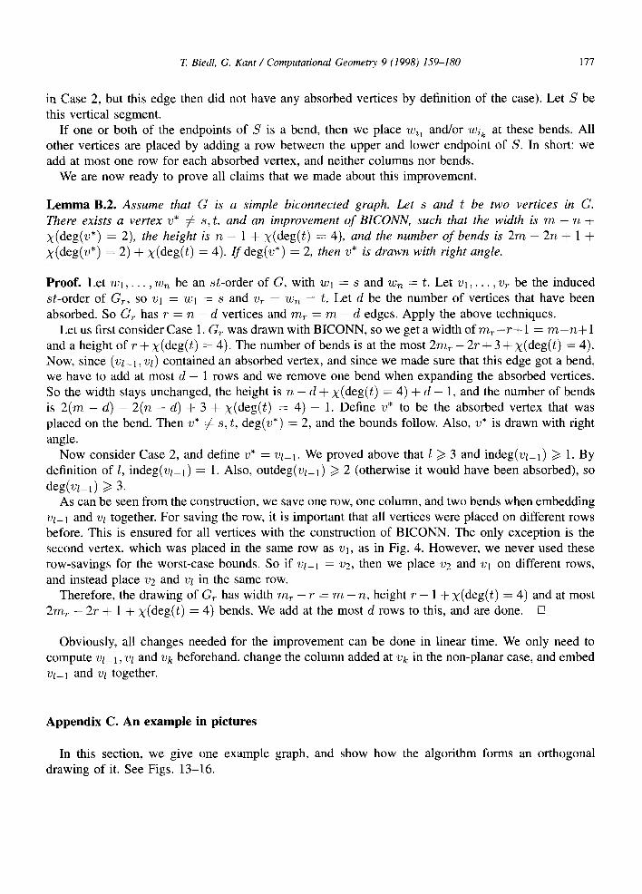
in Case 2, but this edge then did not have any absorbed vertices by definition of the case). Let S be

this vertical segment. I f one or both of the endpoints of S is a bend, then we place wi, and/or wi k at these bends. All

other vertices are placed by adding a row between the upper and lower endpoint of S. In short: we add at most one row for each absorbed vertex, and neither columns nor bends.

We are now ready to prove all claims that we made about this improvement .

L e m m a B.2. Assume that G is a simple biconnected graph. Let s and t be two vertices in G. There exists a vertex v* ~ s, t, and an improvement of BICONN, such that the width is m - n + x(deg(v*) = 2), the height is n - 1 ÷ x (deg ( t ) = 4), and the number of bends is 2 m - 2n + 1 + x (deg (v*) = 2) + x (deg ( t ) = 4). I f deg(v*) = 2, then v* is drawn with right angle.

Proof . Let w l , . . . , w,z be an s t -order of G, with 2/) 1 = 8 and wn = t. Let vl , . . . , v~ be the induced s t -order of Gr , so Vl = wl = s and v~ = wn = t. Let d be the number of vertices that have been

absorbed. So G~ has r = n - d vertices and m~ = m - d edges. Apply the above techniques. Let us first consider Case 1. G~ was drawn with BICONN, so we get a width of m ~ - r + 1 = m - n + 1

and a height o f r + x (deg ( t ) = 4). The number of bends is at the most 2m~ - 2 r + 3 + x (deg ( t ) = 4). Now, since (vl-1, vl) contained an absorbed vertex, and since we made sure that this edge got a bend, we have to add at most d - 1 rows and we remove one bend when expanding the absorbed vertices. So the width stays unchanged, the height is n - d + x (deg( t ) = 4) + d - 1, and the number of bends is 2 ( m - d) - 2 (n - d) + 3 + x (deg ( t ) = 4) - 1. Define v* to be the absorbed vertex that was placed on the bend. Then v* ¢ s, t, deg(v*) = 2, and the bounds follow. Also, v* is drawn with right

angle. Now consider Case 2, and define v* = Vt-l . We proved above that I >~ 3 and indeg(vz_l) ~> 1. By

definition of l, indeg(vz_l) = 1. Also, outdeg(vl_ l ) >~ 2 (otherwise it would have been absorbed), so

deg(v/_l) /> 3. As can be seen f rom the construction, we save one row, one column, and two bends when embedding

~ol-1 and vz together. For saving the row, it is important that all vertices were placed on different rows before. This is ensured for all vertices with the construction of BICONN. The only except ion is the second vertex, which was placed in the same row as Vl, as in Fig. 4. However , we never used these

row-savings for the worst-case bounds. So if vt-1 = v2, then we place v2 and Vl on different rows, and instead place v2 and vl in the same row.

Therefore, the drawing of G~ has width m~ - r = m - n, height r - 1 + x (deg ( t ) = 4) and at most 2m~ - 2 r + 1 + x (deg ( t ) = 4) bends. We add at the most d rows to this, and are done. []

Obviously, all changes needed for the improvement can be done in linear time. We only need to compute vt_ l, vz and vk beforehand, change the column added at vk in the non-planar case, and embed

vl-1 and vt together.

Appendix C. An example in pictures

In this section, we give one example graph, and show how the algori thm forms an orthogonal drawing of it. See Figs. 13-16.

178 T. Biedl, G. Kant / Computational Geomet~ 9 (1998) 159-180

Go

(b) G~

G1,1

Fig. 13. (a) The input-graph. It is not 4-regular, and not biconnected. We choose one vertex to be drawn as final vertex (shown white). (b) We split the graph into its blocks. Along the way, we determine for each block which vertex should be drawn as final vertex (shown white for each block).

Go G1 ~ G 1 , 1

(a) am

~ G | ,1

Go G1

(b) a~

Fig. 14. (a) We embed each component with BICONN and the improvement, using the white vertex as the last vertex. Each block turns out to be planar. (b) For the cutvertex in Go, we add a new column and a bend, and move it such that it is drawn with right angle.

GO G1

(a)

+

G1,1 % G1.2

(b)

GoUG1 uGl,1 uG1,2

T - T

i

Fig. 15. (a) We merge Gl.i and GI.2 into GI. We have to rotate GI,I by 180 degree. (b) We merge the obtained subgraph into Go. We have to rotate the subgraph.

T. Biedl, G. Kant/Computational Geometr), 9 (1998) 159-180 179

(a)

T- Y

(b)

Fig. 16. (a) Finally, we merge G~, the subgraph connected by a bridge. (b) After a suitable compaction step, the picture is significantly reduced in size.

References

[ 1] T. Biedl, New lower bounds for orthogonal graph drawing, in: Proc. Graph Drawing '95, Lecture Notes in Computer Science 1027, Springer, Berlin, 1996, pp. 28-39.

[2] T. Biedl, Optimal orthogonal drawings of triconnected plane graphs, in: Proc. Scandinavian Workshop on Algorithm Theory, Lecture Notes in Computer Science 1097, Springer, Berlin, 1996, pp. 333-344.

[3] T. Biedl, Improved orthogonal drawings of 3-graphs, in: Fiala, Kranakis, Sack (eds.), Proc. 8th Canadian Conference on Computational Geometry, International Informatics Series 5, Carleton University Press, 1996, pp. 295-299.

[4] T. Biedl, Optimal orthogonal drawings of connected plane graphs, in: Fiala, Kranakis, Sack (eds.), Proc. 8th Canadian Conference on Computational Geometry, International Informatics Series 5, Carleton University Press, 1996, pp. 306-311.

[5] N. Chiba, T. Nishizeki, S. Abe, T. Ozawa, A linear algorithm for embedding planar graphs using PQ-trees, J. Comput. System Sci. 30 (1985) 54-76.

[6] G. Di Battista, P. Eades, R. Tamassia, I.G. Tollis, Algorithms for automatic graph drawing: an annotated bibliography, Computational Geometry: Theory and Applications 4 (5) (1994) 235-282.

[7] G. Di Battista, A. Garg, G. Liotta, R. Tamassia, E. Tassinari, E Vargiu, An experimental comparison of four graph drawing algorithms, Computational Geometry: Theory and Applications 7 (5-6) (1997) 303-325.

[8] P.E Dietz, D.D. Sleator, Two algorithms for maintaining order in a list, in: Proc. 19th Annual ACM Symp. Theory of Computing, 1987, pp. 365-372.

[9] S. Even, G. Granot, Rectilinear planar drawings with few bends in each edge, Manuscript, Faculty of Comp. Science, the Technion, Haifa, Israel, 1993.

[10] S. Even, R.E. Tarjan, Computing an st-numbering, Theoret. Comput. Sci. 2 (1976) 436-441. [11] M. Formann, F. Wagner, The VLSI layout problem in various embedding models, in: Graph-Theoretic

Concepts in Comp. Science (16th Workshop WG '90), Springer, Berlin, 1992, pp. 130-139. [12] U. F013meier, M. Kaufmann, Drawing high degree graphs with low bend numbers, in: Proc. Graph Drawing

'95, Lecture Notes in Computer Science 1027, Springer, Berlin, 1996, pp. 254-266.


[13] A. Garg, R. Tamassia, On the computational complexity of upward and rectilinear planarity testing, in: Proc. Graph Drawing '94, Lecture Notes in Computer Science 894, Springer, Berlin, 1995, pp. 286-297.

[14] A. Garg, R. Tamassia, A new minimum cost flow algorithm with applications to graph drawing, in: Proc. Graph Drawing '96, Lecture Notes in Computer Science 1190, Springer, Berlin, 1997, pp. 201-216.

[15] G. Kant, Drawing planar graphs using the canonical ordering, Algorithmica 16 (1996) 4-32. [16] M.R. Kramer, J. van Leeuwen, The complexity of wire routing and finding minimum area layouts for

arbitrary VLSI circuits, in: EE Preparata (ed.), Advances in Computer Research, Vol. 2: VLSI Theory, JAI Press, Reading, MA, 1984, pp. 129-146.

[17] A. Lempel, S. Even, I. Cederbaum, An algorithm for planarity testing of graphs, in: Theory of Graphs, Internat. Symp. Rome, 1966, pp. 215-232.

[18] T. Lengauer, Combinatorial Algorithms for Integrated Circuit Layout, Teubner/Wiley, Stuttgart/Chichester, 1990.

[ 19] Y. Liu, A. Morgana, B. Simeone, General theoretical results on rectilinear embeddability of graphs, Acta Math. Appl. Sinica 7 (1991) 187-191.

[20] B. Madden, E Madden, S. Powers, M. Himsolt, Portable graph layout and editing, in: Proc. Graph Drawing '95, Lecture Notes in Computer Science 1024, Springer, Berlin, 1996, pp. 385-395.

[21] A. Papakostas, I.G. Tollis, A pairing technique for area-efficient orthogonal drawings, in: Proc. Graph Drawing '96, Lecture Notes in Computer Science 1190, Springer, Berlin, 1997, pp. 355-370.

[22] M. Schaffter, Drawing graphs on rectangular grids, Discrete Appl. Math. 63 (1995) 75-89. [23] J. Storer, On minimal node-cost planar embeddings, Networks 14 (1984) 181-212. [24] R. Tamassia, On embedding a graph in the grid with the minimum number of bends, SIAM J. Comput. 16

(1987) 421-444. [25] R. Tamassia, I.G. Tollis, Efficient embedding of planar graphs in linear time, in: Proc. IEEE Internat. Symp.

on Circuits and Systems, Philadelphia, 1987, pp. 495-498. [26] R. Tamassia, I.G. Tollis, J.S. Vitter, Lower bounds for planar orthogonal drawings of graphs, Inform. Process.

Lett. 39 (1991) 35-40. [27] L.G. Valiant, On non-linear lower bounds in computational complexity, in: Proc. 7th Symp. on Theory of

Computing, 1975, pp. 45-53.

a better heuristic for orthogonal graph drawings

Documents