7

A Bayesian Network to Predict Vulnerability to Sea-Level Rise: Data Report

Data Series 2011–601 U.S. Department of the Interior U.S. Geological Survey

Cover. Cover caption goes here

A Bayesian Network to Predict Vulnerability to Sea-Level Rise: Data Report

By Benjamin T. Gutierrez, Nathaniel G. Plant, and E. Robert Thieler

Data Series 2011–601 U.S. Department of the Interior U.S. Geological Survey

U.S. Department of the Interior KEN SALAZAR, Secretary

U.S. Geological Survey Marcia K. McNutt, Director

U.S. Geological Survey, Reston, Virginia 2011

For product and ordering information: World Wide Web: http://www.usgs.gov/pubprod Telephone: 1-888-ASK-USGS

For more information on the USGS—the Federal source for science about the Earth, its natural and living resources, natural hazards, and the environment—visit http://www.usgs.gov or call 1-888-ASK-USGS

For an overview of USGS information products, including maps, imagery, and publications, visit http://www.usgs.gov/pubprod

To order this and other USGS information products, visit http://store.usgs.gov

The datasets in this report have been approved for release and publication by the Director of the USGS. Although these datasets have been subjected to rigorous review and are substantially complete, the USGS reserves the right to revise the data pursuant to further analysis and review. Futhermore, they are released on condition that neither the USGS nor the United States Government may be held liable for any damages resulting from their authorized or unauthorized use.

Any use of trade, product, or firm names is for descriptive purposes only and does not imply endorsement by the U.S. Government. Although this report is in the public domain, permission must be secured from the individual copyright owners to reproduce any copyrighted material contained within this report.

Suggested citation: Gutierrez, B.T., Plant, N.G., and Thieler, E.R., 2011, A Bayesian network to predict vulnerability to sea-level rise: data report. U.S. Geological Survey Data Series 601, available at: http://pubs.usgs.gov/ds/601.

5

Contents Abstract .......................................................................................................................................................................... 7 Introduction .................................................................................................................................................................... 7 Development of the Bayesian Network .......................................................................................................................... 8

Bayesian Networks ..................................................................................................................................................... 8 The THK99 Dataset .................................................................................................................................................. 10 Mapping Bayesian Network Predictions ................................................................................................................... 12

Geospatial Data ........................................................................................................................................................... 12 Metadata ...................................................................................................................................................................... 13 Acknowledgments ........................................................................................................................................................ 13 References Cited ......................................................................................................................................................... 14

Figures Figure 1. The structure of the Bayesian Network (BN) used for this study ..................................................................... 9 Figure 2. Map of shoreline change rates for the U.S. Atlantic coast showing the spatial extent of the

THK99 dataset ................................................................................................................................................ 11 Figure 3.Maps of the U.S. Atlantic coast showing the posterior probability of shoreline change less

than -1 m/yr ..................................................................................................................................................... 12

Tables Table 1. Variables used in the BN. ............................................................................ ……………9

6

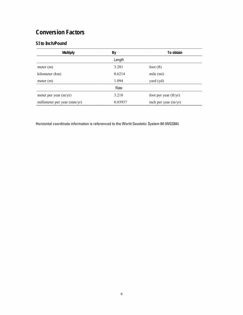
Conversion Factors SI to Inch/Pound

Multiply By To obtain

Length

meter (m) 3.281 foot (ft)

kilometer (km) 0.6214 mile (mi)

meter (m) 1.094 yard (yd)

Rate

meter per year (m/yr) 3.218 foot per year (ft/yr)

millimeter per year (mm/yr) 0.03937 inch per year (in/yr)

Horizontal coordinate information is referenced to the World Geodetic System 84 (WGS84).

7

A Bayesian Network to Predict Vulnerability to Sea-Level Rise: Data Report

By Benjamin T. Gutierrez, Nathaniel G. Plant, and E. Robert Thieler

Abstract During the 21st century, sea-level rise is projected to have a wide range of effects on coastal

environments, development, and infrastructure. Consequently, there has been an increased focus on developing modeling or other analytical approaches to evaluate potential impacts to inform coastal management. This report provides the data that were used to develop and evaluate the performance of a Bayesian network designed to predict long-term shoreline change due to sea-level rise. The data include local rates of relative sea-level rise, wave height, tide range, geomorphic classification, coastal slope, and shoreline-change rate compiled as part of the U.S. Geological Survey Coastal Vulnerability Index for the U.S. Atlantic coast. In this project, the Bayesian network is used to define relationships among driving forces, geologic constraints, and coastal responses. Using this information, the Bayesian network is used to make probabilistic predictions of shoreline change in response to different future sea-level-rise scenarios.

Introduction Despite the limitations of forecasting shoreline changes far into the future, sets of basic data such as

historical shoreline positions have been used to identify and evaluate the potential for future shoreline changes (Thieler and Hammar-Klose, 1999; hereafter abbreviated as THK99). This work was conducted as part of a study to evaluate how a probabilistic approach using a Bayesian network (BN) (Jensen and Nielsen, 2007) could be used to calculate the probability of long-term shoreline change given knowledge of the rate of relative sea-level rise and other basic physical parameters. The Bayesian approach has been used in the artificial intelligence, medical-, and ecological-research communities to evaluate and translate scientific information and (or) expert judgments into probabilistic terms (see review by Berger, 2000). More recently, BNs have been used in the earth and environmental sciences, particularly to address ecological questions (Borsuk and others, 2004; Wilson and others, 2008). The Bayesian statistical framework is ideal for datasets derived from historical to modern observations of phenomena such as long-term shoreline change. For this study, a BN provided a means of integrating observations to evaluate the relationships between forcing factors (for example, rate of sea-level rise, wave height, or tidal range), and coastal responses (for example, shoreline-change rate). The predictions can also be used to estimate outcome uncertainty that can be expressed both in numbers (for example, 90 percent) and established likelihood terms (for example, “very likely,” Intergovernmental Panel on Climate Change, 2007). Communicating information about the effects of sea-level-rise in terms of probability may improve scientists’ ability to support decisionmaking and address specific management questions regarding the effects of sea-level rise.

This report provides the data that were used by the U.S. Geological Survey to develop and evaluate a BN to calculate probabilities of long-term shoreline change (Gutierrez and others, 2011). The BN was developed and tested over a two-year period in 2009 and 2010 and implemented using a commercial software package, Netica (Norsys, 2009). Input data were extracted from the Coastal Vulnerability Index (CVI, Thieler and Hammar-Klose, 1999), which was developed to describe physical processes or conditions at specific locations along the U.S. Atlantic coast. The data included with this report provide probabilities of long-term shoreline change computed using the BN developed for this study. A detailed account of the results of this analysis can be found in Gutierrez and others (2011).

8

Development of the Bayesian Network This section reviews the methodology that was used to implement the Bayesian network. The first part

provides a brief review of Bayes theorem and how a Bayesian network was structured to address long-term shoreline change. The second part reviews the data that were used to calculate probabilities of shoreline change using the Bayesian network.

Bayesian Networks A Bayesian network provides a framework to evaluate the probability of a specific outcome based on

causal relationships among variables identified by users. Bayes’ theorem relates the probability of one event R given the occurrence of another event O (Bayes, 1763; Gelman and others, 2004):

)()()|(

)|(j

iijji Op

RpROpORp

⋅=

On the left side of this equation, p(Ri|Oj) is the conditional probability of a particular response, Ri, given a set of observations Oj. For example, a particular response might be the joint occurrence of a particular rate of sea-level rise and a particular rate of shoreline change. The ith response scenario refers to the number of input scenarios that can be considered. Likewise, the jth observation refers to the set of observations that are considered for each scenario, such as wave height, rate of sea-level rise, or one of the other variables. On the right side of this equation, p(Oj|Ri) is the likelihood of the observations for a known response. This term indicates the strength of the correlation between observation and response, such as the rate of sea-level rise and shoreline change. The correlation is high if the observations are accurate and if response variables are sensitive to the observed variables. The second term in the numerator p(Ri) is the prior probability of the response, which is the probability of a particular response integrated over all expected observation scenarios. The denominator p(Oj) is a normalization factor to account for the likelihood of the observations.

The Norsys software package Netica (Norsys, 1992–2009) was used to construct a BN for the data from THK99. The network was configured on the basis of simple causal relationships among six variables (fig. 1). These variables, often referred to as decision nodes in a BN, were divided into three categories: driving forces, geological boundary conditions, and a response variable used as a vulnerability indicator. The rate of relative sea-level rise, wave height, and tidal range are considered driving forces. The geomorphic setting and coastal slope are considered geological boundary conditions. The shoreline-change rate was the response variable. Each node (that is, variable) is resolved by five classes, or binned values, corresponding to risk categories defined in THK99 (table 1). We structured the BN to reflect our understanding of how the variables influence long-term shoreline change.

9

Figure 1. Diagram showing the structure of the Bayesian network (BN) used for this study. The rate of relative sea-level rise, mean wave height, and tidal range were assumed to be driving forces; the coastal slope and geomorphic setting were assumed to be geological boundary conditions; and the shoreline-change rate was considered to be the vulnerability indicator.

Table 1. Variables used in the Bayesian network.

Variable Binned values 1 2 3 4 5

Geomorphology1 1 – Very low risk– Rocky, cliffs along

coasts, fjords

2 – Low risk– Medium cliffs, indented coasts

3 – Moderate risk– Low cliffs, glacial

drift, alluvial plains

4 – High risk– Cobble beaches,

estuarine and lagoonal coasts

5 – Very high risk– Barrier beaches,

sand beaches, salt marsh, mud flats,

deltas, mangroves, coral reefs

Shoreline change (m/yr) > 2.0 1.0 – 2.0 -1.0 – 1.0 -2.0 – -1.0 < -2.0

Coastal slope (%) > 0.2 0.2 – 0.07 0.07 – 0.04 0.04 – 0.025 < 0.025 Relative sea-level change (mm/yr) < 1.8 1.8 – 2.5 2.5 – 2.95 2.95 – 3.16 > 3.16

Mean wave height (m) < 0.55 0.55 – 0.85 0.85 – 1.05 1.05 – 1.25 > 1.25

Mean tidal range (m) > 6.0 4.1 – 6.0 2.0 – 4.0 1.0 – 1.9 < 1.0

1The geomorphology ranking is based on the sea-level rise vulnerability classification used by THK99. [m/yr, meters per year; %, percent; mm/yr, millimeters per year; m, meters; >, greater than; <, less than]

10

The THK99 Dataset The six variables used in THK99 were defined for the coastlines of the continental United States (fig. 1,

table 1). The THK99 data were originally gridded to a shoreline data layer at about 5-km resolution that included inland coastal waterways. For this study, we focused on the U.S. Atlantic coast and removed data points for inland waterways for which no shoreline-change data were available; this coverage matched the original extent of the data in Dolan and others (1985), which were used to provide the long-term shoreline-change rates in THK99. The input data include the ocean-facing shores of the U.S. Atlantic coast from the Canadian border to Key West, Florida, and portions of Chesapeake and Delaware Bays. Data in each node of the BN are binned according to the same risk categories defined in THK99 (table 1). The resulting BN predictions are applicable at the same spatial scale as the input. The variables are described briefly below and explained in detail in THK99.

Rate of Relative Sea-Level Rise—Computed by fitting a linear trend to National Ocean Service (NOS) long-term (50–more than 100 years) tide-gauge observations and interpolating alongshore between stations. In the BN used here, the rate of sea-level rise is assumed to influence the geomorphic setting and the shoreline- change rate.

Mean Wave Height—Computed from U.S. Army Corps of Engineers Wave Information Studies (WIS) hindcast data (Hubertz and others 1996) and interpolated alongshore between WIS stations. Wave height reflects the wave climatology and potential sediment transport in a particular area and is assumed to influence the geomorphic setting and the shoreline-change rate.

Mean Tidal Range—Computed from NOS tide gauges and interpolated alongshore between stations. Tidal range influences the characteristics of coastal landforms such as barrier islands (Hayes, 1979). THK99 and Morton (2003) also point out that in areas where storm surges may occur, regions with low tidal ranges can have higher potential for inundation and consequently greater risk of dune breaching than areas with higher tidal range. The tidal range is assumed to influence the geomorphic setting and the shoreline change rate.

Geomorphic Setting—Based on an ordinal vulnerability classification of sea-level rise by Gornitz and Kanciruk (1989) and modified by THK99 to include the division of barrier islands into transgressive and regressive types (Nummedal, 1983). Coastal landforms develop as a result of the interaction of many factors. It is assumed that the rate of sea-level rise, mean wave height, mean tidal range, and coastal slope all contribute to the development of a given coastal landform that can be identified as a distinct geomorphic setting and that the geomorphic setting influences the shoreline-change rate. Simplifying the THK99 definitions in this paper, geomorphic settings 1 and 2 represent very low and low vulnerability settings, setting 3 moderate vulnerability, and settings 4 and 5 high and very high vulnerability, respectively (table 1).

Coastal Slope—Computed from gridded National Geophysical Data Center and U.S. Navy topographic and bathymetric data extending approximately 50 km landward and seaward of the local shoreline. Coastal slope is a measure of the gradient of the substrate on which the local geomorphology has formed and which influences the development of coastal landforms in a region (Roy and others, 1994). Coastal slope can affect the shoreline-change rate because shallow gradients can result in greater horizontal displacement per unit rise in sea level (Pilkey and Davis, 1987).

Shoreline-Change Rate—Decadal-to-centennial-scale historical rates of shoreline change based on data compiled by May and others (1983) and Dolan and others (1985) into the Coastal Erosion Information System (CEIS) (May and others, 1982) (fig. 2). The data in CEIS are drawn from a wide variety of sources, including published reports, historical shoreline-change maps, field surveys, and aerial-photo analyses; however, the lack of a standard method among coastal scientists for analyzing shoreline changes (Morton and Miller, 2005) has resulted in the inclusion of data based on a variety of reference features, measurement techniques, and rate-of-change calculations. Thus, while CEIS represents the best data currently available for the entire Atlantic coast in

11

a format amenable to this analysis, actual regional and local erosion rates may differ significantly (compare to May and others, 1983; Dolan and others, 1990). We updated data for the southern shore of Delaware Bay and the northern Chesapeake Bay with shoreline-change rates from Dolan and Peatross (1992); this update was deemed necessary because of possible gridding errors in the original THK99 dataset, which was based on an older shoreline-change dataset (Dolan and others, 1985). In the BN used here, shoreline-change rate is the response variable and is assumed to be influenced by the other variables in the network.

Figure 2. Map showing shoreline-change rates for the U.S. Atlantic coast showing the spatial extent of the dataset that was use as input data for the Bayesian network used in this paper. Negative rates of shoreline change denote erosion.

12

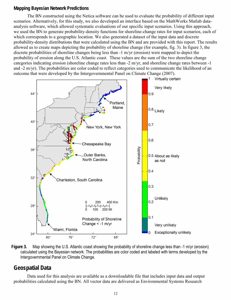
Mapping Bayesian Network Predictions The BN constructed using the Netica software can be used to evaluate the probability of different input

scenarios. Alternatively, for this study, we also developed an interface based on the MathWorks Matlab data-analysis software, which allowed systematic evaluations of our specific input scenarios. Using this approach, we used the BN to generate probability-density functions for shoreline-change rates for input scenarios, each of which corresponds to a geographic location. We also generated a dataset of the input data and discrete probability-density distributions that were calculated using the BN and are provided with this report. The results allowed us to create maps depicting the probability of shoreline change (for example, fig. 3). In figure 3, the discrete probabilities of shoreline changes being less than -1 m/yr (erosion) were mapped to depict the probability of erosion along the U.S. Atlantic coast. These values are the sum of the two shoreline change categories indicating erosion (shoreline change rates less than -2 m/yr, and shoreline change rates between -1 and -2 m/yr). The probabilities are color coded to reflect categories used to communicate the likelihood of an outcome that were developed by the Intergovernmental Panel on Climate Change (2007).

Figure 3. Map showing the U.S. Atlantic coast showing the probability of shoreline change less than -1 m/yr (erosion) calculated using the Bayesian network. The probabilities are color coded and labeled with terms developed by the Intergovernmental Panel on Climate Change.

Geospatial Data Data used for this analysis are available as a downloadable file that includes input data and output

probabilities calculated using the BN. All vector data are delivered as Environmental Systems Research

13

Institute (ESRI) shapefiles in the geographic coordinate system (WGS84) and distributed with Federal Geographic Data Committee (FGDC) compliant metadata in Extensible Markup Language (*.xml) format. Tabular data are delivered as dBase IV (*.dbf) structured files, which can be read with ESRI ArcGIS software as well as many other available spreadsheet programs. Metadata are also provided for all spatial and tabular data in text (*.txt) and FGDC Classic (*.html) format. ESRI ArcCatalog 9.x or higher can also be used to examine the metadata in a variety of additional formats.

The data provided with this report consist of a shapefile and accompanying spreadsheet that contain input data for each location as well as the corresponding output, which consists of probability-density distributions for discrete shoreline-change rates . As described in an earlier section of the report (see “The THK99 Dataset”), the input data were acquired for the Atlantic coast and modified from THK99. Each set of input values for each location was evaluated using the BN to produce the output probability distributions (see “Mapping Bayesian Network Predictions”).

The input data consist of seven fields: a. identifier (ID) b. Decimal longitude c. Decimal latitude d. Slope (percent) e. Geomorphology f. Rate of relative sea-level rise (mm/yr) g. Mean wave height (m) h. Tidal range (m) i. Erosion rate (m/yr)

The output probability distributions consist of five classes corresponding to the five fields (fig. 2):

h. pErosion2—probability of shoreline change less than -2 m/yr i. pErosion1—probability of shoreline change less than -1 m/yr to -2 m/yr j. pStable—probability of shoreline change less than 1 m/yr to -1 m/yr k. pAccretion1—probability of shoreline change greater than 1 m/yr to 2 m/yr l. pAccretion2—probability of shoreline change greater than 2 m/yr

Metadata Link to Metadata in on-line version: for review see “ProbSLC_AtlanticData.html”

Acknowledgments This work was funded by the U.S. Geological Survey Coastal and Marine Geology and Global Change

Research Programs. We thank Jane Denny, Jeffrey List, and VeeAnn Cross of the USGS Woods Hole Coastal their review and feedback on this report.

14

References Cited

Bayes, Thomas, 1763, An essay towards solving a problem in the doctrine of chances: Philosophical Transactions of the Royal Society of London, p. 330–418. (Reprinted by Barnard, G.A., 1958, Biometrika, v. 45, p. 293-315.)

Berger, J.O., 2000, Bayesian analysis—a look at today and thoughts of tomorrow: Journal of the American

Statistical Association, v. 95, no. 452 , p. 1269–1276. Borsuk, M.E., Stow, C.A., and Reckhow, K.H., 2004, A Bayesian network of eutrophication models for

synthesis, prediction, and uncertainty analysis: Ecological Modelling, v. 173, p. 219–239. Dolan, R., Anders, F., and Kimball, S., 1985, Coastal erosion and accretion: National Atlas of the United States

of America, U.S. Geological Survey, Reston, Virginia, 1 sheet. Dolan, Robert, Trossbach, Susan, and Buckley, Michael, 1990, New shoreline erosion data for the mid-Atlantic

coast: Journal of Coastal Research, v. 6, no. 2, p. 471–477. Dolan, R., and Peatross, J., 1992, Data supplement to the U.S. Geological Survey 1:2,000,000-scale map of

shoreline erosion and accretion of the mid-Atlantic coast: U.S. Geological Survey, Open-File Report 92–377, Reston, Va.,, 116 p.

Gelman, A., Carlin, J.B., Stern, H.S., and Rubin, D.B., 2004, Bayesian data analysis (2nd ed.): Chapman &

Hall, New York, 668 p. Gornitz, V.M., and Kanciruk, P., 1989, Assessment of global coastal hazards from sea level rise, in Coastal

Zone ’89, Proceedings of the Sixth Symposium on Coastal and Ocean Management: Charleston, S.C., American Society of Civil Engineers, N.Y., p. 1345–1359.

Gutierrez, B.T., Plant, N.G., and Thieler, E.R., 2011, A Bayesian network to predict coastal vulnerability to sea-

level rise: Journal of Geophysical Research EarthSurface, 116, doi:10.1029/2010JF001891. Hayes, M.O., 1979, Barrier island morphology as a function of tidal and wave regime, in Leatherman, S.P., ed.,

Barrier islands: from the Gulf of St. Lawrence to the Gulf of Mexico: Academic Press, New York, N.Y., p. 211–236.

Hubertz, J. M., Thompson, E. F., and Wang, H. V. 1996, Wave information studies of U.S. coastlines—

Annotated bibliography on coastal and ocean data assimilation: WIS Report 36, U.S. Army Engineer Waterways Experiment Station, Vicksburg, Miss., 31 p.

International Panel on Climate Change, 2007, Climate change 2007—The physical science basis, in

Contribution of working group I to the fourth assessment report of the Intergovernmental Panel on Climate Change, Solomon, S., Qin, D., Manning, M., Chen, Z., Marquis, M., Avery, K.B., Tignor, M., and. Miller, H.L., eds.: Cambridge University Press, Cambridge, United Kingdom, and New York, New York.

Jensen, F.V., and Nielsen, T.D., 2007, Bayesian networks and decision graphs: SpringerVerlag, New York,

N.Y., 447 p. May, S. K., Dolan, R., and Hayden, B.P., 1983, Erosion of U.S. shorelines: EOS Transactions of the American

Geophysical Union, v. 64, no. 35, p. 521–523. May, S. K., Kimball, W. H., Grady, N., and Dolan, R., 1982, CEIS—The coastal erosion information system:

Shore and Beach, v. 50, p. 19–26.

15

Morton, R.A., 2003, An overview of coastal land loss—with emphasis on the southeastern United States, U.S.

Geological Survey Open-File Report 03–337, 29 p. Morton, R.A., and Miller, T.L., 2005, National assessment of shoreline change, part 2—Historical shoreline

changes and associated coastal land loss along the U.S. Southeast Atlantic Coast: U.S. Geological Survey Open-File Report, 2005–1401, 35 p.

Norsys, 1992–2009, Netica verison 4.09, www.norsys.com. Last accessed, March, 2010. Nummedal, D. 1983, Barrier islands, in Komar, P.D., Handbook of coastal processes and erosion: CRC Press,

Boca Raton, Fl., p. 77–121. Pilkey, O.H. and T. W. Davis (1987), An analysis of coastal recession models—NorthCarolina coast, in D.

Nummedal, D., Pilkey, O.H., and Howard, J.D., eds., Sea-level fluctuation and coastal evolution: Tulsa, Okla., Society of Economic Paleontologists and Mineralogists, pp. 59–68.

Roy, P.S., Cowell, P.J., Ferland, M.A., and Thom, B.G., 1994, Wave-dominated coasts, in Carter, R.W.G., and

Woodroffe, C.D., eds., Late Quaternary shoreline morphodynamics: Cambridge, Cambridge University Press, pp.121–186.

Thieler, E.R. and Hammar-Klose, E.S., 1999, National assessment of coastal vulnerability to future sea-level

rise--Preliminary results for the U.S. Atlantic Coast: U.S. Geological Survey Open File Report 99–593, 1 sheet. (Also available online at http://pubs.usgs.gov/of/of99–593.)

Wilson, D.S., Stoddard, M.A., and Puettmann, 2008, Monitoring amphibian populations with incomplete survey

information using a Bayesian probabilistic model: Ecological Modelling, v. 214, p. 210–218.

For more information concerning this report, contact Director

U.S. Geological Survey Woods Hole Coastal and Marine Science Center 384 Woods Hole Road Quissett Campus Woods Hole, MA 02543-1598 WHSC_science_director@usgs.gov 508-548-8700 or 508-457-2200 or visit our Web site at http://woodshole.er.usgs.gov

Gutierrez and others— A

Bayesian N

etwork to Predict Vulnerability to Sea-Level Rise: D

ata Report—Data Series 2011-601