a bayesian estimate of the cmb-large scale...
TRANSCRIPT

A Bayesian estimate of the CMB-large scale structure
cross correlationEdivaldo Moura SantosInstituto de Física - USP
in collaboration withF. C. Carvalho (UERN), M. Penna Lima (APC), C. P. Novaes (ON), C. A. Wuensche (INPE)
10th PPC, 11-15 July 2016, ICTP-SAIFR, São Paulo1
arXiv:1512.00641 (to appear in ApJ)

Motivation• Cross-correlation can give us some additional hints on the current universe’s
accelerated phase• Crossed signal can be estimated with several different estimators• There have been many measurements in the past with quite different levels of
significances, from null to marginal to highly significant claims (depending on the estimators and data set)
• Highest signals have been seen when localised super-structures were used
2

Integrated Sachs-Wolfe (ISW) effect
3
• gravitational potentials vary with time in an accelerated universe
• superclusters x CMB hotspots• supervoids x CMB coldspots
Positive correlations:

The CMB-LSS cross correlation
4
• But from Poisson eq. in Fourier space (large-k, no-radiation limit):
• Secondary CMB anisotropy due to time variable potential:
• Galaxy overdensity fluctuations:
• One can then write a two-point correlation function in harmonic space:
Main observables here! (Ctt, Cgg, Ctg)
gµ⌫ =
0
BB@
�1� 2 0 0 00 a2(1 + 2�) 0 00 0 a2(1 + 2�) 00 0 0 a2(1 + 2�)
1
CCA
perturbed metric in an expanding flat universe:
kernels:Cxy
`
⌘ h�x
(n̂)�y
(n̂0)i = 2
⇡
Zdkk2W x
`
(k)W y
`
(k)P (k)

Expected signals for a ΛCDM cosmology
5
0
1000
2000
3000
4000
5000
6000
10 100 1000
ℓ (ℓ
+1) C
ℓtt / 2/
[µK2 ]
ℓ
RCDM
10-5
10-4
10-3
10-2
10-1
10 100
Cℓgg
ℓ
RCDM + selection 1RCDM + selection 2RCDM + selection 3RCDM + selection 4
0
0.05
0.1
0.15
0.2
0.25
10 100
ℓ (ℓ
+1) C
ℓtg /
2/ [µ
K]
ℓ
RCDM + selection 1RCDM + selection 2RCDM + selection 3RCDM + selection 4
LSS autocorrelationCMB autocorrelation
cross-correlation

A Bayesian question
6
Question: What is the likelihood for observing the fluctuations of the combined set of a CMB temperature and a galaxy contrast map?
C = S+N
Answer (for a flat prior):
S = diag(S0,S1, · · · ,S`max
) S` =
✓Stt` Stg
`
Stg` Sgg
`
◆
L =
1p(2⇡)Np
(detC)
exp
�1
2
dTC�1d
�
In harmonic spacesignal covariance matrix:
Np-pixel mapsd =( )CMB map
galaxy map
Hypothesis: Gaussian fluctuations (primordial and
instrumental noise)

Gibbs sampling equationsfluctuation field
si+1 - P (s|Si,d)
Si+1 - P (S|si+1)
(primordial signal)
(signal covariance)
Build a Markov chain whose stationary distribution is the desired likelihood.
Each step in the chain involves the draw of a S matrix and a signal map:
7
For a Markov chain with nG steps, one can use a Blackwell-Rao estimator:
The log of the Blackwell-Rao likelihood can then be maximized to get maximum likelihood values for the power spectrum
(S(0), s(0)), ..., (S(nb), s(nb))| {z }burn-in phase
, ..., (S(i), s(i)), ...
L ' 1
nG
nGX
i=1
Pi(S|s)
d=As+n
beam noise
signal

8
Two-Micron All Sky Survey (2MASS)• eXtended Source Catalog (XSC)
• near IR
• position + photometry + basic shape information
• 1,647,599 resolved objects: 97% galaxies
Publicly available from: ftp://ftp.ipac.caltech.edu/pub/2mass/allsky/

2MASS redshift distributions
9
• 2MASS is a shallow catalog
• peak sensitivity around z=0.1
Final parameterisation:
• redshift distribution from Schechter parameters that best fit K20 magnitudes:
l.o.s. comoving volume
luminosity function
PRD69 (2004) 083524
0
5
10
15
20
25
30
0 0.05 0.1 0.15 0.2 0.25 0.3
Nor
mal
ized
sel
ectio
n fu
nctio
n
redshift
2MPZ photoz (12.0<K20<12.5)2MPZ photoz (12.5<K20<13.0)2MPZ photoz (13.0<K20<13.5)2MPZ photoz (13.5<K20<13.9)
Afshordi 1Afshordi 2Afshordi 3Afshordi 4
K20 ! K 020 = K20 �Ak (Ak = 0.367⇥ E(B � V ))
• KS-band 2.16 micron magnitudes (k_m_i20c) corrected for extinction using Schlegel maps (ApJ 500, 525 (1998)):

2MASS low resolution contrast maps
10

10-5
10-4
10-3
10-2
10-1
10 100
12.0 ≤ K20 < 12.5 (XSC band 1)
Cℓgg
ℓ
halofit
linear theory
2MASS autocorrelations and the galaxy bias
11
10-5
10-4
10-3
10-2
10-1
10 100
12.5 ≤ K20 < 13.0 (XSC band 2)
Cℓgg
ℓ
halofit
linear theory
10-5
10-4
10-3
10-2
10-1
10 100
13.0 ≤ K20 < 13.5 (XSC band 3)
Cℓgg
ℓ
halofit
linear theory
10-5
10-4
10-3
10-2
10-1
10 100
13.5 ≤ K20 ≤ 14.0 (XSC band 4)
Cℓgg
ℓ
halofit
linear theory

10-5
10-4
10-3
10-2
10-1
10 100
12.0 ≤ K20 < 12.5 (XSC band 1)
Cℓgg
ℓ
halofit
linear theory
2MASS autocorrelations and the galaxy bias
12
10-5
10-4
10-3
10-2
10-1
10 100
12.5 ≤ K20 < 13.0 (XSC band 2)
Cℓgg
ℓ
halofit
linear theory
10-5
10-4
10-3
10-2
10-1
10 100
13.0 ≤ K20 < 13.5 (XSC band 3)
Cℓgg
ℓ
halofit
linear theory
10-5
10-4
10-3
10-2
10-1
10 100
13.5 ≤ K20 ≤ 14.0 (XSC band 4)
Cℓgg
ℓ
halofit
linear theory
�8 = 0.78

Noise into the WMAP9 channels
W1 Nobs map
• WMAP 3 cleanest channels: (Q (40 GHz) / V (60 GHz) / W (90 GHz))
13
Average noise power over 100 sky realisations
W1 temperature (I) map
0
500
1000
1500
2000
2500
3000
3500
4000
100 200 300 400 500 600 700 800 900 1000
ℓ (ℓ +
1) C
ℓ / 2
π [m
icro
K2 ]
ℓ
QVW
ILCQ-noiseV-noiseW-noise
• Average noise power fairly well understood, but pixel-to-pixel correlation hard to model
• Gaussian noise model in pixel space:
Data publicly available from: http://lambda.gsfc.nasa.gov
�2 =�20
Nobs

WMAP9 low resolution (r5) maps
14
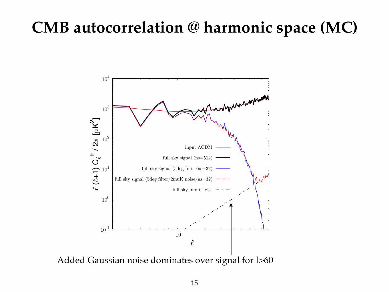
CMB autocorrelation @ harmonic space (MC)
10-1
100
101
102
103
104
10
ℓ (ℓ
+1) C
ℓtt / 2/
[µK2 ]
ℓ
input RCDM
full sky signal (ns=512)
full sky signal (5deg filter/ns=32)
full sky signal (5deg filter/2muK noise/ns=32)
full sky input noise
15
Added Gaussian noise dominates over signal for l>60

16
mean
fluctuation
mean+fluc
CMB LSS MC
0
1000
2000
3000
4000
ℓ (ℓ
+ 1
) Cℓtt /
2 π
[µK2 ]
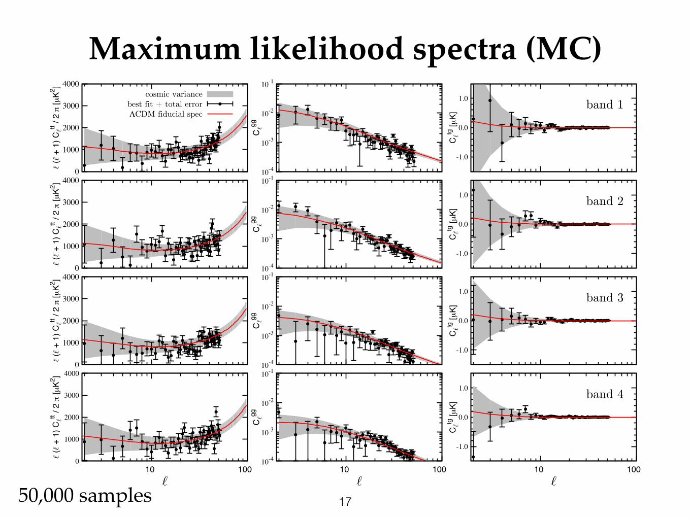
cosmic variancebest fit + total errorΛCDM fiducial spec
0
1000
2000
3000
4000
ℓ (ℓ
+ 1
) Cℓtt /
2 π
[µK2 ]
0
1000
2000
3000
4000
ℓ (ℓ
+ 1
) Cℓtt /
2 π
[µK2 ]
0
1000
2000
3000
4000
10 100
ℓ (ℓ
+ 1
) Cℓtt /
2 π
[µK2 ]
ℓ
10-4
10-3
10-2
10-1
Cℓgg
10-4
10-3
10-2
10-1
Cℓgg
-1.0
0.0
1.0 band 1
Cℓtg
[µK]
-1.0
0.0
1.0 band 2
Cℓtg
[µK]
-1.0
0.0
1.0 band 3
Cℓtg
[µK]
-1.0
0.0
1.0
10 100
band 4
Cℓtg
[µK]
ℓ
10-4
10-3
10-2
10-1
Cℓgg
10-4
10-3
10-2
10-1
10 100
Cℓgg
ℓ
Maximum likelihood spectra (MC)
1750,000 samples

0
1000
2000
3000
4000
ℓ (ℓ
+ 1
) Cℓtt /
2 π
[µK2 ]
cosmic variancesystematics
best fit + total errorΛCDM fiducial spec.
0
1000
2000
3000
4000
ℓ (ℓ
+ 1
) Cℓtt /
2 π
[µK2 ]
0
1000
2000
3000
4000
ℓ (ℓ
+ 1
) Cℓtt /
2 π
[µK2 ]
0
1000
2000
3000
4000
10 100
ℓ (ℓ
+ 1
) Cℓtt /
2 π
[µK2 ]
ℓ
10-4
10-3
10-2
10-1
Cℓgg
10-4
10-3
10-2
10-1
Cℓgg
-0.8
-0.5
-0.2
0.0
0.2
0.5
0.8
band 1
Cℓtg
[µK]
-0.8
-0.5
-0.2
0.0
0.2
0.5
0.8
band 2
Cℓtg
[µK]
-0.8
-0.5
-0.2
0.0
0.2
0.5
0.8
band 3
Cℓtg
[µK]
-0.8
-0.5
-0.2
0.0
0.2
0.5
0.8
10 100
band 4
Cℓtg
[µK]
ℓ
10-4
10-3
10-2
10-1
Cℓgg
10-4
10-3
10-2
10-1
10 100
Cℓgg
ℓ
Final spectra and systematics (data)
1850,000 samples drawn red line is not a fitscale invariant Jeffrey’s prior used
arXiv:1512.00641

0
1000
2000
3000
4000
ℓ (ℓ
+ 1
) Cℓtt /
2 π
[µK2 ]
cosmic variancesystematics
best fit + total errorΛCDM fiducial spec.
0
1000
2000
3000
4000
ℓ (ℓ
+ 1
) Cℓtt /
2 π
[µK2 ]
0
1000
2000
3000
4000
ℓ (ℓ
+ 1
) Cℓtt /
2 π
[µK2 ]
0
1000
2000
3000
4000
10 100
ℓ (ℓ
+ 1
) Cℓtt /
2 π
[µK2 ]
ℓ
10-4
10-3
10-2
10-1
Cℓgg
10-4
10-3
10-2
10-1
Cℓgg
-0.8
-0.5
-0.2
0.0
0.2
0.5
0.8
band 1
Cℓtg
[µK]
-0.8
-0.5
-0.2
0.0
0.2
0.5
0.8
band 2
Cℓtg
[µK]
-0.8
-0.5
-0.2
0.0
0.2
0.5
0.8
band 3
Cℓtg
[µK]
-0.8
-0.5
-0.2
0.0
0.2
0.5
0.8
10 100
band 4
Cℓtg
[µK]
ℓ
10-4
10-3
10-2
10-1
Cℓgg
10-4
10-3
10-2
10-1
10 100
Cℓgg
ℓ
Final spectra and systematics (data)
1950,000 samples
We also get a low CMB quadrupole (l=2) value
arXiv:1512.00641

Likelihood 1d slices
20
Likelihoods are too broad for low-l multipoles: cosmic variance dominated
0.0
0.5
1.0 ℓ=2lik
elih
ood
b1b2b3b4
ℓ=3 ℓ=4
0.0
0.5
1.0 ℓ=5
likel
ihoo
d ℓ=6 ℓ=7
0.0
0.5
1.0
-0.4 -0.2 0.0 0.2 0.4
ℓ=8
likel
ihoo
d
Cℓtg [µK]
-0.4 -0.2 0.0 0.2 0.4
ℓ=9
Cℓtg [µK]
-0.4 -0.2 0.0 0.2 0.4
ℓ=10
Cℓtg [µK]

Summary
21
• ISW is an additional tool for late time acceleration studies
• Likelihood for combined CMB-galaxy map estimated via Gibbs
sampling and maximised
• Gibbs chain validated with Monte Carlo control samples
• Systematics associated to the sampling algorithm estimated: they
are not the dominant contribution to the uncertainty
• For a shallow catalog like 2MASS, cosmic variance is the main
source of uncertainty
• Future: use Planck as CMB map and deeper surveys like SDSS.