a bayesian approach for learning and planning in partially
TRANSCRIPT
Journal of Machine Learning Research 12 (2011) 1655-1696 Submitted 10/08; Revised 11/10; Published 5/11
A Bayesian Approach for Learning and Planning in PartiallyObservable Markov Decision Processes
Stephane Ross [email protected] InstituteCarnegie Mellon UniversityPittsburgh, PA, USA 15213
Joelle Pineau [email protected] of Computer ScienceMcGill UniversityMontreal, PQ, Canada H3A 2A7
Brahim Chaib-draa [email protected] Science & Software Engineering DeptLaval UniversityQuebec, PQ, Canada G1K 7P4
Pierre Kreitmann [email protected]
Department of Computer ScienceStanford UniversityStanford, CA, USA 94305
Editor: Satinder Baveja
Abstract
Bayesian learning methods have recently been shown to provide an elegant solution tothe exploration-exploitation trade-off in reinforcement learning. However most investiga-tions of Bayesian reinforcement learning to date focus on the standard Markov DecisionProcesses (MDPs). The primary focus of this paper is to extend these ideas to the caseof partially observable domains, by introducing the Bayes-Adaptive Partially ObservableMarkov Decision Processes. This new framework can be used to simultaneously (1) learna model of the POMDP domain through interaction with the environment, (2) track thestate of the system under partial observability, and (3) plan (near-)optimal sequences ofactions. An important contribution of this paper is to provide theoretical results showinghow the model can be finitely approximated while preserving good learning performance.We present approximate algorithms for belief tracking and planning in this model, as wellas empirical results that illustrate how the model estimate and agent’s return improve asa function of experience.Keywords: reinforcement learning, Bayesian inference, partially observable Markov de-cision processes
1. Introduction
Robust decision-making is a core component of many autonomous agents. This generallyrequires that an agent evaluate a set of possible actions, and choose the best one for itscurrent situation. In many problems, actions have long-term consequences that must be
c©2011 Stephane Ross, Joelle Pineau, Brahim Chaib-draa and Pierre Kreitmann.
Ross, Pineau, Chaib-draa and Kreitmann
considered by the agent; it is not useful to simply choose the action that looks the best inthe immediate situation. Instead, the agent must choose its actions by carefully tradingoff their short-term and long-term costs and benefits. To do so, the agent must be able topredict the consequences of its actions, in so far as it is useful to determine future actions.In applications where it is not possible to predict exactly the outcomes of an action, theagent must also consider the uncertainty over possible future events.
Probabilistic models of sequential decision-making take into account such uncertaintyby specifying the chance (probability) that any future outcome will occur, given any currentconfiguration (state) of the system, and action taken by the agent. However, if the modelused does not perfectly fit the real problem, the agent risks making poor decisions. This iscurrently an important limitation in practical deployment of autonomous decision-makingagents, since available models are often crude and incomplete approximations of reality.Clearly, learning methods can play an important role in improving the model as experienceis acquired, such that the agent’s future decisions are also improved.
In the past few decades, Reinforcement Learning (RL) has emerged as an elegant andpopular technique to handle sequential decision problems when the model is unknown (Sut-ton and Barto, 1998). Reinforcement learning is a general technique that allows an agent tolearn the best way to behave, that is, such as to maximize expected return, from repeatedinteractions in the environment. A fundamental problem in RL is that of exploration-exploitation: namely, how should the agent chooses actions during the learning phase, inorder to both maximize its knowledge of the model as needed to better achieve the objectivelater (i.e., explore), and maximize current achievement of the objective based on what isalready known about the domain (i.e., exploit). Under some (reasonably general) condi-tions on the exploratory behavior, it has been shown that RL eventually learns the optimalaction-select behavior. However, these conditions do not specify how to choose actions suchas to maximize utilities throughout the life of the agent, including during the learning phase,as well as beyond.
Model-based Bayesian RL is an extension of RL that has gained significant interest fromthe AI community recently as it provides a principled approach to tackle the problem ofexploration-exploitation during learning and beyond, within the standard Bayesian inferenceparadigm. In this framework, prior information about the problem (including uncertainty)is represented in parametric form, and Bayesian inference is used to incorporate any newinformation about the model. Thus the exploration-exploitation problem can be handled asan explicit sequential decision problem, where the agent seeks to maximize future expectedreturn with respect to its current uncertainty on the model. An important limitation of thisapproach is that the decision-making process is significantly more complex since it involvesreasoning about all possible models and courses of action. In addition, most work to dateon this framework has been limited to cases where full knowledge of the agent’s state isavailable at every time step (Dearden et al., 1999; Strens, 2000; Duff, 2002; Wang et al.,2005; Poupart et al., 2006; Castro and Precup, 2007; Delage and Mannor, 2007).
The primary contribution of this paper is an extension of the model-based Bayesianreinforcement learning to partially observable domains with discrete representations.1 Insupport of this, we introduce a new mathematical model, called the Bayes-Adaptive POMDP
1. A preliminary version of this model was described by Ross et al. (2008a). The current paper providesan in-depth development of this model, as well as novel theoretical analysis and new empirical results.
1656

Bayes-Adaptive POMDPs
(BAPOMDP). This is a model-based Bayesian RL approach, meaning that the frameworkmaintains a posterior over the parameters of the underlying POMDP domain.2 We deriveoptimal algorithms for belief tracking and finite-horizon planning in this model. However,because the size of the state space in a BAPOMD can be countably infinite, these are, for allpractical purposes, intractable. We therefore dedicate substantial attention to the problemof approximating the BAPOMDP model. We provide theoretical results for bounding thestate space while preserving the value function. These results are leveraged to derive anovel belief monitoring algorithm, which is used to maintain a posterior over both modelparameters, and state of the system. Finally, we describe an online planning algorithmwhich provides the core sequential decision-making component of the model. Both thebelief tracking and planning algorithms are parameterized so as to allow a trade-off betweencomputational time and accuracy, such that the algorithms can be applied in real-timesettings.
An in-depth empirical validation of the algorithms on challenging real-world scenariosis outside the scope of this paper, since our focus here is on the theoretical properties of theexact and approximative approaches. Nonetheless we elaborate a tractable approach andcharacterize its performance in three contrasting problem domains. Empirical results showthat the BAPOMDP agent is able to learn good POMDP models and improve its returnas it learns better model estimates. Experiments on the two smaller domains illustrateperformance of the novel belief tracking algorithm, in comparison to the well-known Monte-Carlo approximation methods. Experiments on the third domain confirm good planningand learning performance on a larger domain; we also analyze the impact of the choice ofprior on the results.
The paper is organized as follows. Section 2 presents the models and methods neces-sary for Bayesian reinforcement learning in the fully observable case. Section 3 extendsthese ideas to the case of partially observable domains, focusing on the definition of theBAPOMDP model and exact algorithms. Section 4 defines a finite approximation of theBAPOMDP model that could be used to be solved by finite offline POMDP solvers. Sec-tion 5 presents a more tractable approach to solving the BAPOMDP model based on onlinePOMDP solvers. Section 6 illustrates the empirical performance of the latter approach onsample domains. Finally, Section 7 discusses related Bayesian approaches for simultaneousplanning and learning in partially observable domains.
2. Background and Notation
In this section we discuss the problem of model-based Bayesian reinforcement learning inthe fully observable case, in preparation for the extension of these ideas to the partiallyobservable case which is presented in Section 3. We begin with a quick review of MarkovDecision Processes. We then present the models and methods necessary for Bayesian RL inMDPs. This literature has been developing over the last decade, and we aim to provide abrief but comprehensive survey of the models and algorithms in this area. Readers interestedin a more detailed presentation of the material should seek additional references (Suttonand Barto, 1998; Duff, 2002).
2. This is in contrast to model-free Bayesian RL approaches, which maintain a posterior over the valuefunction, for example, Engel et al. (2003, 2005); Ghavamzadeh and Engel (2007b).
1657
Ross, Pineau, Chaib-draa and Kreitmann
2.1 Markov Decision Processes
We consider finite MDPs as defined by the following n-tuple (S,A, T,R, γ):
States: S is a finite set of states, which represents all possible configurations of thesystem. A state is essentially a sufficient statistic of what occurred in the past, suchthat what will occur in the future only depends on the current state. For example, ina navigation task, the state is usually the current position of the agent, since its nextposition usually only depends on the current position, and not on previous positions.
Actions: A is a finite set of actions the agent can make in the system. These actions mayinfluence the next state of the system and have different costs/payoffs.
Transition Probabilities: T : S × A × S → [0, 1] is called the transition function. Itmodels the uncertainty on the future state of the system. Given the current states, and an action a executed by the agent, T sas
′specifies the probability Pr(s′|s, a)
of moving to state s′. For a fixed current state s and action a, T sa· defines aprobability distribution over the next state s′, such that
∑s′∈S T
sas′ = 1, for all(s, a). The definition of T is based on the Markov assumption, which states thatthe transition probabilities only depend on the current state and action, that is,Pr(st+1 = s′|at, st, . . . , a0, s0) = Pr(st+1 = s′|at, st), where at and st denote respec-tively the action and state at time t. It is also assumed that T is time-homogenous,that is, the transition probabilities do not depend on the current time: Pr(st+1 =s′|at = a, st = s) = Pr(st = s′|at−1 = a, st−1 = s) for all t.
Rewards: R : S × A → R is the function which specifies the reward R(s, a) obtained bythe agent for doing a particular action a in current state s. This models the imme-diate costs (negative rewards) and payoffs (positive rewards) incurred by performingdifferent actions in the system.
Discount Factor: γ ∈ [0, 1) is a discount rate which allows a trade-off between short-termand long-term rewards. A reward obtained t-steps in the future is discounted by thefactor γt. Intuitively, this indicates that it is better to obtain a given reward now,rather than later in the future.
Initially, the agent starts in some initial state, s0 ∈ S. Then at any time t, the agentchooses an action at ∈ A, performs it in the current state st, receives the reward R(st, at)and moves to the next state st+1 with probability T statst+1 . This process is iterated untiltermination; the task horizon can be specified a priori, or determined by the discount factor.
We define a policy, π : S → A, to be a mapping from states to actions. The optimalpolicy, denoted π∗, corresponds to the mapping which maximizes the expected sum of dis-counted rewards over a trajectory. The value of the optimal policy is defined by Bellman’sequation:
V ∗(s) = maxa∈A
[R(s, a) + γ
∑s′∈S
T sas′V ∗(s′)
].
The optimal policy at a given state, π∗(s), is defined to be the action that maximizes thevalue at that state, V ∗(s). Thus the main objective of the MDP framework is to accurately
1658

Bayes-Adaptive POMDPs
estimate this value function, so as to then obtain the optimal policy. There is a largeliterature on the computational techniques that can be leveraged to solve this problem. Agood starting point is the recent text by Szepesvari (2010).
A key aspect of reinforcement learning is the issue of exploration. This corresponds tothe question of determining how the agent should choose actions while learning about thetask. This is in contrast to the phase called exploitation, through which actions are selectedso as to maximize expected reward with respect to the current value function estimate. Theissues of value function estimation and exploration are assumed to be orthogonal in muchof the MDP literature. However in many applications, where data is expensive or difficultto acquire, it is important to consider the rewards accumulated during the learning phase,and to try to take this cost-of-learning into account in the optimization of the policy.
In RL, most practical work uses a variety of heuristics to balance the exploration andexploitation, including for example the well-known ε-greedy and Boltzmann strategies. Themain problem with such heuristic methods is that the exploration occurs randomly and isnot focused on what needs to be learned.
More recently, it has been shown that it is possible for an agent to reach near-optimalperformance with high probability using only a polynomial number of steps (Kearns andSingh, 1998; Brafman and Tennenholtz, 2003; Strehl and Littman, 2005), or alternately tohave small regret with respect to the optimal policy (Auer and Ortner, 2006; Tewari andBartlett, 2008; Auer et al., 2009). Such theoretical results are highly encouraging, and insome cases lead to algorithms which exhibit reasonably good empirical performance.
2.2 Bayesian Learning
Bayesian Learning (or Bayesian Inference) is a general technique for learning the unknownparameters of a probability model from observations generated by this model. In Bayesianlearning, a probability distribution is maintained over all possible values of the unknownparameters. As observations are made, this probability distribution is updated via Bayes’rule, and probability density increases around the most likely parameter values.
Formally, consider a random variable X with probability density fX|Θ over its domainX parameterized by the unknown vector of parameters Θ in some parameter space P. LetX1, X2, · · · , Xn be a random i.i.d. sample from fX|Θ. Then by Bayes’ rule, the posteriorprobability density gΘ|X1,X2,...,Xn(θ|x1, x2, . . . , xn) of the parameters Θ = θ, after the obser-vations of X1 = x1, X2 = x2, · · · ,Xn = xn, is:
gΘ|X1,X2,...,Xn(θ|x1, x2, . . . , xn) =gΘ(θ)
∏ni=1 fX|Θ(xi|θ)∫
P gΘ(θ′)∏ni=1 fX|Θ(xi|θ′)dθ′
,
where gΘ(θ) is the prior probability density of Θ = θ, that is, gΘ over the parameter spaceP is a distribution that represents the initial belief (or uncertainty) on the values of Θ. Notethat the posterior can be defined recursively as follows:
gΘ|X1,X2,...,Xn(θ|x1, x2, . . . , xn) =gΘ|X1,X2,...,Xn−1
(θ|x1, x2, . . . , xn−1)fX|Θ(xn|θ)∫P gΘ|X1,X2,...,Xn−1
(θ′|x1, x2, . . . , xn−1)fX|Θ(xn|θ′)dθ′,
1659

Ross, Pineau, Chaib-draa and Kreitmann
so that whenever we get the nth observation of X, denoted xn, we can compute the newposterior distribution gΘ|X1,X2,...,Xn from the previous posterior gΘ|X1,X2,...,Xn−1
.In general, updating the posterior distribution gΘ|X1,X2,...,Xn is difficult due to the need
to compute the normalization constant∫P gΘ(θ)
∏ni=1 fX|Θ(xi|θ)dθ. However, for conjugate
family distributions, updating the posterior can be achieved very efficiently with a simpleupdate of the parameters defining the posterior distribution (Casella and Berger, 2001).
Formally, consider a particular class G of prior distributions over the parameter spaceP, and a class F of likelihood functions fX|Θ over X parameterized by parameters Θ ∈ P,then F and G are said to be conjugate if for any choice of prior gΘ ∈ G, likelihood fX|Θ ∈ Fand observation X = x, the posterior distribution gΘ|X after observation of X = x is alsoin G.
For example, the Beta distribution3 is conjugate to the Binomial distribution.4 ConsiderX ∼ Binomial(n, p) with unknown probability parameter p, and consider a prior Beta(α, β)over the unknown value of p. Then following an observation X = x, the posterior over p isalso Beta distributed and is defined by Beta(α+ x, β + n− x).
Another important issue with Bayesian methods is the need to specify a prior. While theinfluence of the prior tends to be negligible when provided with a large amount of data, itschoice is particularly important for any inference and decision-making performed when onlya small amount of data has been observed. In many practical problems, informative priorscan be obtained from domain knowledge. For example many sensors and actuators usedin engineering applications have specified confidence intervals on their accuracy providedby the manufacturer. In other applications, such as medical treatment design or portfoliomanagement, data about the problem may have been collected for other tasks, which canguide the construction of the prior.
In the absence of any knowledge, uninformative priors can be specified. Under suchpriors, any inference done a posteriori is dominated by the data, that is, the influence ofthe prior is minimal. A common uninformative prior consists of using a distribution thatis constant over the whole parameter space, such that every possible parameter has equalprobability density. From an information theoretic point of view, such priors have maximumentropy and thus contain the least amount of information about the true parameter (Jaynes,1968). However, one problem with such uniform priors is that typically, under different re-parameterization, one has different amounts of information about the unknown parameters.A preferred uninformative prior, which is invariant under reparameterization, is Jeffreys’prior (Jeffreys, 1961).
The third issue of concern with Bayesian methods concerns the convergence of the poste-rior towards the true parameter of the system. In general, the posterior density concentratesaround the parameters that have highest likelihood of generating the observed data in thelimit. For finite parameter spaces, and for smooth families with continuous finite dimen-sional parameter spaces, the posterior converges towards the true parameter as long as theprior assigns non-zero probability to every neighborhood of the true parameter. Hence inpractice, it is often desirable to assign non-zero prior density over the full parameter space.
3. Beta(α, β) is defined by the density function f(p|α, β) ∝ pα−1(1 − p)β−1 for p ∈ [0, 1] and parametersα, β ≥ 0.
4. Binomial(n, p) is defined by the density function f(k|n, p) ∝ pk(1 − p)n−k for k ∈ {0, 1, . . . , n} andparameters p ∈ [0, 1],n ∈ N.
1660

Bayes-Adaptive POMDPs
It should also be noted that if multiple parameters within the parameter space cangenerate the observed data with equal likelihood, then the posterior distribution will usuallybe multimodal, with one mode surrounding each equally likely parameter. In such cases,it may be impossible to identify the true underlying parameter. However for practicalpurposes, such as making predictions about future observations, it is sufficient to identifyany of the equally likely parameters.
Lastly, another concern is how fast the posterior converges towards the true parameters.This is mostly influenced by how far the prior is from the true parameter. If the prior ispoor, that is, it assigns most probability density to parameters far from the true parameters,then it will take much more data to learn the correct parameter than if the prior assignsmost probability density around the true parameter. For such reasons, a safe choice is touse an uninformative prior, unless some data is already available for the problem at hand.
2.3 Bayesian Reinforcement Learning in Markov Decision Processes
Work on model-based Bayesian reinforcement learning dates back to the days of Bellman,who studied this problem under the name of Adaptive control processes (Bellman, 1961).An excellent review of the literature on model-based Bayesian RL is provided in Duff (2002).This paper outlines, where appropriate, more recent contributions in this area.
As a side note, model-free BRL methods also exist (Engel et al., 2003, 2005; Ghavamzadehand Engel, 2007a,b). Instead of representing the uncertainty on the model, these methodsexplicitly model the uncertainty on the value function or optimal policy. These methodsmust often rely on heuristics to handle the exploration-exploitation trade-off, but may beuseful in cases where it is easier to express prior knowledge about initial uncertainty on thevalue function or policy, rather than on the model.
The main idea behind model-based BRL is to use Bayesian learning methods to learnthe unknown model parameters of the system, based on what is observed by the agent in theenvironment. Starting from a prior distribution over the unknown model parameters, theagent updates a posterior distribution over these parameters as it performs actions and getsobservations from the environment. Under such a Bayesian approach, the agent can computethe best action-selection strategy by finding the one that maximizes its future expectedreturn under the current posterior distribution, but also considering how this distributionwill evolve in the future under different possible sequences of actions and observations.
To formalize these ideas, consider an MDP (S,A, T,R, γ), where S, A and R are known,and T is unknown. Furthermore, assume that S and A are finite. The unknown parametersin this case are the transition probabilities, T sas
′, for all s, s′ ∈ S, a ∈ A. The model-based
BRL approach to this problem is to start off with a prior, g, over the space of transitionfunctions, T . Now let st = (s0, s1, . . . , st) and at−1 = (a0, a1, . . . , at−1) denote the agent’shistory of visited states and actions up to time t. Then the posterior over transition functionsafter this sequence is defined by:
g(T |st, at−1) ∝ g(T )∏t−1i=0 T
siaisi+1
∝ g(T )∏s∈S,a∈A
∏s′∈S(T sas
′)N
as,s′ (st,at−1)
,
1661
Ross, Pineau, Chaib-draa and Kreitmann
where Nas,s′(st, at−1) =
∑t−1i=0 I{(s,a,s′)}(si, ai, si+1) is the number of times5 the transition
(s, a, s′) occurred in the history (st, at−1). As we can see from this equation, the likelihood∏s∈S,a∈A
∏s′∈S(T sas
′)N
as,s′ (st,at−1) is a product of |S||A| independent Multinomial6 distri-
butions over S. Hence, if we define the prior g as a product of |S||A| independent pri-ors over each distribution over next states T sa·, that is, g(T ) =
∏s∈S,a∈A gs,a(T
sa·), thenthe posterior is also defined as a product of |S||A| independent posterior distributions:g(T |st, at−1) =
∏s∈S,a∈A gs,a(T
sa·|st, at−1), where gs,a(T sa·|st, at−1) is defined as:
gs,a(T sa·|st, at−1) ∝ gs,a(T sa·)∏s′∈S
(T sas′)N
as,s′ (st,at−1)
.
Furthermore, since the Dirichlet distribution is the conjugate of the Multinomial, itfollows that if the priors gs,a(T sa·) are Dirichlet distributions for all s, a, then the posteriorsgs,a(T sa·|st, at−1) will also be Dirichlet distributions for all s, a. The Dirichlet distributionis the multivariate extension of the Beta distribution and defines a probability distributionover discrete distributions. It is parameterized by a count vector, φ = (φ1, . . . , φk), whereφi ≥ 0, such that the density of probability distribution p = (p1, . . . , pk) is defined asf(p|φ) ∝
∏ki=1 p
φi−1i . If X ∼ Multinomialk(p,N) is a random variable with unknown
probability distribution p = (p1, . . . , pk), and Dirichlet(φ1, . . . , φk) is a prior over p, thenafter the observation of X = n, the posterior over p is Dirichlet(φ1+n1, . . . , φk+nk). Hence,if the prior gs,a(T sa·) is Dirichlet(φas,s1 , . . . , φ
as,s|S|
), then after the observation of history(st, at−1), the posterior gs,a(T sa·|st, at−1) is Dirichlet(φas,s1 + Na
s,s1(st, at−1), . . . , φas,s|S| +Nas,s|S|
(st, at−1)). It follows that if φ = {φas,s′ |a ∈ A, s, s′ ∈ S} represents the set of allDirichlet parameters defining the current prior/posterior over T , then if the agent performsa transition (s, a, s′), the posterior Dirichlet parameters φ′ after this transition are simplydefined as:
φ′as,s′ = φas,s′ + 1,φ′a′
s′′,s′′′ = φa′s′′,s′′′ , ∀(s′′, a′, s′′′) 6= (s, a, s′).
We denote this update by the function U , where U(φ, s, a, s′) returns the set φ′ as updatedin the previous equation.
Because of this convenience, most authors assume that the prior over the transition func-tion T follows the previous independence and Dirichlet assumptions (Duff, 2002; Deardenet al., 1999; Wang et al., 2005; Castro and Precup, 2007). We also make such assumptionsthroughout this paper.
2.3.1 Bayes-Adaptive MDP Model
The core sequential decision-making problem of model-based Bayesian RL can be cast asthe problem of finding a policy that maps extended states of the form (s, φ) to actionsa ∈ A, such as to maximize the long-term rewards of the agent. If this decision problem
5. We use I() to denote the indicator function.
6. Multinomialk(p,N) is defined by the density function f(n|p,N) ∝Qki=1 p
nii for ni ∈ {0, 1, . . . , N} such
thatPki=1 ni = N , parameters N ∈ N, and p is a discrete distribution over k outcomes.
1662
Bayes-Adaptive POMDPs
can be modeled as an MDP over extended states (s, φ), then by solving this new MDP, wewould find such an optimal policy. We now explain how to construct this MDP.
Consider a new MDP defined by the tuple (S′, A, T ′, R′, γ). We define the new set ofstates S′ = S × T , where T = {φ ∈ N|S|2|A||∀(s, a) ∈ S × A,
∑s′∈S φ
ass′ > 0}, and A is the
original action space. Here, the constraints on the set T of possible count parameters φ areonly needed to ensure that the transition probabilities are well defined. To avoid confusion,we refer to the extended states (s, φ) ∈ S′ as hyperstates. Also note that the next informa-tion state φ′ only depends on the previous information state φ and the transition (s, a, s′)that occurred in the physical system, so that transitions between hyperstates also exhibitthe Markov property. Since we want the agent to maximize the rewards it obtains in thephysical system, the reward function R′ should return the same reward as in the physicalsystem, as defined in R. Thus we define R′(s, φ, a) = R(s, a). The only remaining issue isto define the transition probabilities between hyperstates. The new transition function T ′
must specify the transition probabilities T ′(s, φ, a, s′, φ′) = Pr(s′, φ′|s, a, φ). By the chainrule, Pr(s′, φ′|s, a, φ) = Pr(s′|s, a, φ) Pr(φ′|s, a, s′, φ). Since the update of the informationstate φ to φ′ is deterministic, then Pr(φ′|s, a, s′, φ) is either 0 or 1, depending on whetherφ′ = U(φ, s, a, s′) or not. Hence Pr(φ′|s, a, s′, φ) = I{φ′}(U(φ, s, a, s′)). By the law of totalprobability, Pr(s′|s, a, φ) =
∫Pr(s′|s, a, T, φ)f(T |φ)dT =
∫T sas
′f(T |φ)dT , where the inte-
gral is carried over transition function T , and f(T |φ) is the probability density of transitionfunction T under the posterior defined by φ. The term
∫T sas
′f(T |φ)dT is the expecta-
tion of T sas′
for the Dirichlet posterior defined by the parameters φas,s1 , . . . , φas,s|S|
, which
corresponds toφas,s′P
s′′∈S φas,s′′
. Thus it follows that:
T ′(s, φ, a, s′, φ′) =φas,s′∑
s′′∈S φas,s′′
I{φ′}(U(φ, s, a, s′)).
We now have a new MDP with a known model. By solving this MDP, we can find theoptimal action-selection strategy, given a posteriori knowledge of the environment. Thisnew MDP has been called the Bayes-Adaptive MDP (Duff, 2002) or the HyperMDP (Castroand Precup, 2007).
Notice that while we have assumed that the reward function R is known, this BRLframework can easily be extended to the case where R is unknown. In such a case, onecan proceed similarly by using a Bayesian learning method to learn the reward functionR and add the posterior parameters for R in the hyperstate. The new reward function R′
then becomes the expected reward under the current posterior over R, and the transitionfunction T ′ would also model how to update the posterior over R, upon observation of anyreward r. For brevity of presentation, it is assumed that the reward function is knownthroughout this paper. However, the frameworks we present in the following sections canalso be extended to handle cases where the rewards are unknown, by following a similarreasoning.
2.3.2 Optimality and Value Function
The Bayes-Adaptive MDP (BAMDP) is just a conventional MDP with a countably infinitenumber of states. Fortunately, many theoretical results derived for standard MDPs carry
1663
Ross, Pineau, Chaib-draa and Kreitmann
over to the Bayes-Adaptive MDP model (Duff, 2002). Hence, we know there exists anoptimal deterministic policy π∗ : S′ → A, and that its value function is defined by:
V ∗(s, φ) = maxa∈A[R′(s, φ, a) + γ
∑(s′,φ′)∈S′ T
′(s, φ, a, s′, φ′)V ∗(s′, φ′)]
= maxa∈A
[R(s, a) + γ
∑s′∈S
φas,s′P
s′′∈S φas,s′′
V ∗(s′,U(φ, s, a, s′))].
(1)
This value function is defined over an infinite number of hyperstates, therefore, in prac-tice, computing V ∗ exactly for all hyperstates is unfeasible. However, since the summationover S is finite, we observe that from one given hyperstate, the agent can transit only toa finite number of hyperstates in one step. It follows that for any finite planning horizont, one can compute exactly the optimal value function for a particular starting hyperstate.However the number of reachable hyperstates grows exponentially with the planning hori-zon.
2.3.3 Planning Algorithms
We now review existing approximate algorithms for estimating the value function in theBAMDP. Dearden et al. (1999) proposed one of the first Bayesian model-based explorationmethods for RL. Instead of solving the BAMDP directly via Equation 1, the Dirichletdistributions are used to compute a distribution over the state-action values Q∗(s, a), inorder to select the action that has the highest expected return and value of information(Dearden et al., 1998). The distribution over Q-values is estimated by sampling MDPsfrom the posterior Dirichlet distribution, and then solving each sampled MDP to obtaindifferent sampled Q-values. Re-sampling and importance sampling techniques are proposedto update the estimated Q-value distribution as the Dirichlet posteriors are updated.
Rather than using a maximum likelihood estimate for the underlying process, Strens(2000) proposes to fully represent the posterior distribution over process parameters. Hethen uses a greedy behavior with respect to a sample from this posterior. By doing so, heretains each hypothesis over a period of time, ensuring goal-directed exploratory behaviorwithout the need to use approximate measures or heuristic exploration as other approachesdid. The number of steps for which each hypothesis is retained limits the length of explo-ration sequences. The results of this method is then an automatic way of obtaining behaviorwhich moves gradually from exploration to exploitation, without using heuristics.
Duff (2001) suggests using Finite-State Controllers (FSC) to represent compactly theoptimal policy π∗ of the BAMDP and then finding the best FSC in the space of FSCs ofsome bounded size. A gradient descent algorithm is presented to optimize the FSC anda Monte-Carlo gradient estimation is proposed to make it more tractable. This approachpresupposes the existence of a good FSC representation for the policy.
For their part, Wang et al. (2005) present an online planning algorithm that estimatesthe optimal value function of the BAMDP (Equation 1) using Monte-Carlo sampling. Thisalgorithm is essentially an adaptation of the Sparse Sampling algorithm (Kearns et al.,1999) to BAMDPs. However instead of growing the tree evenly by looking at all actionsat each level of the tree, the tree is grown stochastically. Actions are sampled accordingto their likelihood of being optimal, according to their Q-value distributions (as defined by
1664

Bayes-Adaptive POMDPs
the Dirichlet posteriors); next states are sampled according to the Dirichlet posterior on themodel. This approach requires multiple sampling and solving of MDPs from the Dirichletdistributions to find which action has highest Q-value at each state node in the tree. Thiscan be very time consuming, and so far the approach has only been applied to small MDPs.
Castro and Precup (2007) present a similar approach to Wang et al. However their ap-proach differs on two main points. First, instead of maintaining only the posterior over mod-els, they also maintain Q-value estimates using a standard Q-Learning method. Planning isdone by growing a stochastic tree as in Wang et al. (but sampling actions uniformly instead)and solving for the value estimates in that tree using Linear Programming (LP), insteadof dynamic programming. In this case, the stochastic tree represents sampled constraints,which the value estimates in the tree must satisfy. The Q-value estimates maintained byQ-Learning are used as value estimates for the fringe nodes (thus as value constraints onthe fringe nodes in the LP).
Finally, Poupart et al. (2006) proposed an approximate offline algorithm to solve theBAMDP. Their algorithm, called Beetle, is an extension of the Perseus algorithm (Spaanand Vlassis, 2005) to the BAMDP model. Essentially, at the beginning, hyperstates (s, φ)are sampled from random interactions with the BAMDP model. An equivalent continuousPOMDP (over the space of states and transition functions) is solved instead of the BAMDP(assuming (s, φ) is a belief state in that POMDP). The value function is represented bya set of α-functions over the continuous space of transition functions. Each α-function isconstructed as a linear combination of basis functions; the sampled hyperstates can serve asthe set of basis functions. Dynamic programming is used to incrementally construct the setof α-functions. At each iteration, updates are only performed at the sampled hyperstates,similarly to Perseus (Spaan and Vlassis, 2005) and other Point-Based POMDP algorithms(Pineau et al., 2003).
3. Bayes-Adaptive POMDPs
Despite the sustained interest in model-based BRL, the deployment to real-world applica-tions is limited both by scalability and representation issues. In terms of representation, animportant challenge for many practical problems is in handling cases where the state of thesystem is only partially observable. Our goal here is to show that the model-based BRLframework can be extended to handle partially observable domains. Section 3.1 provides abrief overview of the Partially Observable Markov Decision Process framework. In order toapply Bayesian RL methods in this context, we draw inspiration from the Bayes-AdaptiveMDP framework presented in Section 2.3, and propose an extension of this model, calledthe Bayes-Adaptive POMDP (BAPOMDP). One of the main challenges that arises whenconsidering such an extension is how to update the Dirichlet count parameters when thestate is a hidden variable. As will be explained in Section 3.2, this can be achieved byincluding the Dirichlet parameters in the state space, and maintaining a belief state overthese parameters. The BAPOMDP model thus allows an agent to improve its knowledgeof an unknown POMDP domain through interaction with the environment, but also allowsthe decision-making aspect to be contingent on uncertainty over the model parameters. Asa result, it is possible to define an action-selection strategy which can directly trade-offbetween (1) learning the model of the POMDP, (2) identifying the unknown state, and
1665

Ross, Pineau, Chaib-draa and Kreitmann
(3) gathering rewards, such as to maximize its future expected return. This model offersan alternative framework for reinforcement learning in POMDPs, compared to previoushistory-based approaches (McCallum, 1996; Littman et al., 2002).
3.1 Background on POMDPs
While an MDP is able to capture uncertainty on future outcomes, and the BAMDP is ableto capture uncertainty over the model parameters, both fail to capture uncertainty that canexist on the current state of the system at a given time step. For example, consider a medicaldiagnosis problem where the doctor must prescribe the best treatment to an ill patient. Inthis problem the state (illness) of the patient is unknown, and only its symptoms can beobserved. Given the observed symptoms the doctor may believe that some illnesses are morelikely, however he may still have some uncertainty about the exact illness of the patient.The doctor must take this uncertainty into account when deciding which treatment is bestfor the patient. When the uncertainty is high, the best action may be to order additionalmedical tests in order to get a better diagnosis of the patient’s illness.
To address such problems, the Partially Observable Markov Decision Process (POMDP)was proposed as a generalization of the standard MDP model. POMDPs are able to modeland reason about the uncertainty on the current state of the system in sequential decisionproblems (Sondik, 1971).
A POMDP is defined by a finite set of states S, a finite set of actions A, as well asa finite set of observations Z. These observations capture the aspects of the state whichcan be perceived by the agent. The POMDP is also defined by transition probabilities{T sas′}s,s′∈S,a∈A, where T sas
′= Pr(st+1 = s′|st = s, at = a), as well as observation proba-
bilities {Osaz}s∈S,a∈A,z∈Z where Osaz = Pr(zt = z|st = s, at−1 = a). The reward function,R : S ×A→ R, and discount factor, γ, are as in the MDP model.
Since the state is not directly observed, the agent must rely on the observation and actionat each time step to maintain a belief state b ∈ ∆S, where ∆S is the space of probabilitydistributions over S. The belief state specifies the probability of being in each state giventhe history of action and observation experienced so far, starting from an initial belief b0.It can be updated at each time step using the following Bayes rule:
bt+1(s′) =Os′atzt+1
∑s∈S T
sats′bt(s)∑s′′∈sO
s′′atzt+1∑
s∈S Tsats′′bt(s)
.
A policy π : ∆S → A indicates how the agent should select actions as a function of thecurrent belief. Solving a POMDP involves finding the optimal policy π∗ that maximizes theexpected discounted return over the infinite horizon. The return obtained by following π∗
from a belief b is defined by Bellman’s equation:
V ∗(b) = maxa∈A
[∑s∈S
b(s)R(s, a) + γ∑z∈Z
Pr(z|b, a)V ∗(τ(b, a, z))
],
where τ(b, a, z) is the new belief after performing action a and observation z,and γ ∈ [0, 1)is the discount factor.
A key result by Smallwood and Sondik (1973) shows that the optimal value function fora finite-horizon POMDP is piecewise-linear and convex. It means that the value function
1666
Bayes-Adaptive POMDPs
Vt at any finite horizon t can be represented by a finite set of |S|-dimensional hyperplanes:Γt = {α0, α1, . . . , αm}. These hyperplanes are often called α-vectors. Each defines a linearvalue function over the belief state space, associated with some action, a ∈ A. The value ofa belief state is the maximum value returned by one of the α-vectors for this belief state:
Vt(b) = maxα∈Γt
∑s∈S
α(s)b(s).
The best action is the one associated with the α-vector that returns the best value.The Enumeration algorithm by Sondik (1971) shows how the finite set of α-vectors,
Γt, can be built incrementally via dynamic programming. The idea is that any t-stepcontingency plan can be expressed by an immediate action and a mapping associating a(t-1)-step contingency plan to every observation the agent could get after this immediateaction. The value of the 1-step plans corresponds directly to the immediate rewards:
Γa1 = {αa|αa(s) = R(s, a)},Γ1 =
⋃a∈A Γa1.
Then to build the α-vectors at time t, we consider all possible immediate actions the agentcould take, every observation that could follow, and every combination of (t-1)-step plansto pursue subsequently:
Γa,zt = {αa,z|αa,z(s) = γ∑
s′∈S Tsas′Os
′azα′(s′), α′ ∈ Γt−1},Γat = Γa1 ⊕ Γa,z1t ⊕ Γa,z2t ⊕ . . .⊕ Γ
a,z|Z|t ,
Γt =⋃a∈A Γat ,
where ⊕ is the cross-sum operator.7
Exactly solving the POMDP is usually intractable, except on small domains with onlya few states, actions and observations (Kaelbling et al., 1998). Various approximate al-gorithms, both offline (Pineau et al., 2003; Spaan and Vlassis, 2005; Smith and Simmons,2004) and online (Paquet et al., 2005; Ross et al., 2008c), have been proposed to tackle in-creasingly large domains. However, all these methods require full knowledge of the POMDPmodel, which is a strong assumption in practice. Some approaches do not require knowledgeof the model, as in Baxter and Bartlett (2001), but these approaches generally require someknowledge of a good (and preferably compact) policy class, as well as needing substantialamounts of data.
3.2 Bayesian Learning of a POMDP model
Before we introduce the full BAPOMDP model for sequential decision-making under modeluncertainty in a POMDP, we first show how a POMDP model can be learned via a Bayesianapproach.
Consider an agent in a POMDP (S,A,Z, T,O,R, γ), where the transition function Tand observation function O are the only unknown components of the POMDP model. Letzt = (z1, z2, . . . , zt) be the history of observations of the agent up to time t. Recall also thatwe denote st = (s0, s1, . . . , st) and at−1 = (a0, a1, . . . , at−1) the history of visited states and
7. Let A and B be sets of vectors, then A⊕B = {a+ b|a ∈ A, b ∈ B}.
1667

Ross, Pineau, Chaib-draa and Kreitmann
actions respectively. The Bayesian approach to learning T and O involves starting with aprior distribution over T and O, and maintaining the posterior distribution over T and Oafter observing the history (at−1, zt). Since the current state st of the agent at time t isunknown in the POMDP, we consider a joint posterior g(st, T,O|at−1, zt) over st, T , andO. By the laws of probability and Markovian assumption of the POMDP, we have:
g(st, T,O|at−1, zt) ∝ Pr(zt, st|T,O, at−1)g(T,O, at−1)∝
∑st−1∈St Pr(zt, st|T,O, at−1)g(T,O)
∝∑
st−1∈St g(s0, T,O)∏ti=1 T
si−1ai−1siOsiai−1zi
∝∑
st−1∈St g(s0, T,O)[∏
s,a,s′(Tsas′)N
ass′ (st,at−1)
]×[∏
s,a,z(Osaz)N
asz(st,at−1,zt)
],
where g(s0, T,O) is the joint prior over the initial state s0, transition function T , and ob-servation function O; Na
ss′(st, at−1) =∑t−1
i=0 I{(s,a,s′)}(si, ai, si+1) is the number of times thetransition (s, a, s′) appears in the history of state-action (st, at−1); and Na
sz(st, at−1, zt) =∑ti=1 I{(s,a,z)}(si, ai−1, zi) is the number of times the observation (s, a, z) appears in the his-
tory of state-action-observations (st, at−1, zt). We use proportionality rather than equalityin the expressions above because we have not included the normalization constant.
Under the assumption that the prior g(s0, T,O) is defined by a product of independentpriors of the form:
g(s0, T,O) = g(s0)∏s,a
gsa(T sa·)gsa(Osa·),
and that gsa(T sa·) and gsa(Osa·) are Dirichlet priors defined ∀s, a, then we observe that theposterior is a mixture of joint Dirichlets, where each joint Dirichlet component is parame-terized by the counts corresponding to one specific possible state sequence:
g(st, T,O|at−1, zt) ∝∑
st−1∈St g(s0)c(st, at−1, zt)×[∏s,a,s′(T
sas′)Nass′ (st,at−1)+φa
ss′−1]×[∏
s,a,z(Osaz)N
asz(st,at−1,zt)+ψasz−1
].
(2)
Here, φas· are the prior Dirichlet count parameters for gsa(T sa·), ψas· are the prior Dirichletcount parameters for gsa(Osa·), and c(st, at−1, zt) is a constant which corresponds to thenormalization constant of the joint Dirichlet component for the state-action-observationhistory (st, at−1, zt). Intuitively, Bayes’ rule tells us that given a particular state sequence,it is possible to compute the proper posterior counts of the Dirichlets, but since the statesequence that actually occurred is unknown, all state sequences (and their correspondingDirichlet posteriors) must be considered, with some weight proportional to the likelihoodof each state sequence.
In order to update the posterior online, each time the agent performs an action and getsan observation, it is more useful to express the posterior in recursive form:
g(st, T,O|at−1, zt) ∝∑
st−1∈ST st−1at−1stOstat−1ztg(st−1, T,O|at−2, zt−1).
Hence if g(st−1, T,O|at−2, zt−1) =∑
(φ,ψ)∈C(st−1)w(st−1, φ, ψ)f(T,O|φ, ψ) is a mixtureof |C(st−1)| joint Dirichlet components, where each component (φ, ψ) is parameterized by
1668
Bayes-Adaptive POMDPs
the set of transition counts φ = {φass′ ∈ N|s, s′ ∈ S, a ∈ A} and the set observation countsψ = {ψasz ∈ N|s ∈ S, a ∈ A, z ∈ Z}, then g(st, T,O|at−1, zt) is a mixture of
∏s∈S |C(s)| joint
Dirichlet components, given by:
g(st, T,O|at−1, zt) ∝∑
st−1∈S∑
(φ,ψ)∈C(st−1)w(st−1, φ, ψ)c(st−1, at−1, st, zt−1, φ, ψ)f(T,O|U(φ, st−1, at−1, st),U(ψ, st, at−1, zt)),
where U(φ, s, a, s′) increments the count φass′ by one in the set of counts φ, U(ψ, s, a, z)increments the count ψasz by one in the set of counts ψ, and c(st−1, at−1, st, zt−1, φ, ψ) isa constant corresponding to the ratio of the normalization constants of the joint Dirichletcomponent (φ, ψ) before and after the update with (st−1, at−1, st, zt−1). This last equationgives us an online algorithm to maintain the posterior over (s, T,O), and thus allows theagent to learn about the unknown T and O via Bayesian inference.
Now that we have a simple method of maintaining the uncertainty over both the stateand model parameters, we would like to address the more interesting question of how tooptimally behave in the environment under such uncertainty, in order to maximize futureexpected return. Here we proceed similarly to the Bayes-Adaptive MDP framework definedin Section 2.3.
First, notice that the posterior g(st, T,O|at−1, zt) can be seen as a probability distribu-tion (belief) b over tuples (s, φ, ψ), where each tuple represents a particular joint Dirichletcomponent parameterized by the counts (φ, ψ) for a state sequence ending in state s (i.e., thecurrent state is s), and the probabilities in the belief b correspond to the mixture weights.Now we would like to find a policy π for the agent which maps such beliefs over (s, φ, ψ)to actions a ∈ A. This suggests that the sequential decision problem of optimally behavingunder state and model uncertainty can be modeled as a POMDP over hyperstates of theform (s, φ, ψ).
Consider a new POMDP (S′, A, Z, P ′, R′, γ), where the set of states (hyperstates) is for-mally defined as S′ = S × T ×O, with T = {φ ∈ N|S|2|A||∀(s, a) ∈ S ×A,
∑s′∈S φ
ass′ > 0}
and O = {ψ ∈ N|S||A||Z||∀(s, a) ∈ S × A,∑
z∈Z ψasz > 0}. As in the definition of
the BAMDP, the constraints on the count parameters φ and ψ are only to ensure thatthe transition-observation probabilities, as defined below, are well defined. The actionand observation sets are the same as in the original POMDP. The rewards depend onlyon the state s ∈ S and action a ∈ A (but not the counts φ and ψ), thus we haveR′(s, φ, ψ, a) = R(s, a). The transition and observations probabilities in the BAPOMDPare defined by a joint transition-observation function P ′ : S′×A×S′×Z → [0, 1], such thatP ′(s, φ, ψ, a, s′, φ′, ψ′, z) = Pr(s′, φ′, ψ′, z|s, φ, ψ, a). This joint probability can be factorizedby using the laws of probability and standard independence assumptions:
Pr(s′, φ′, ψ′, z|s, φ, ψ, a)= Pr(s′|s, φ, ψ, a) Pr(z|s, φ, ψ, a, s′) Pr(φ′|s, φ, ψ, a, s′, z) Pr(ψ′|s, φ, ψ, a, s′, φ′, z)= Pr(s′|s, a, φ) Pr(z|a, s′, ψ) Pr(φ′|φ, s, a, s′) Pr(ψ′|ψ, a, s′, z).
As in the Bayes-Adaptive MDP case, Pr(s′|s, a, φ) corresponds to the expectation ofPr(s′|s, a) under the joint Dirichlet posterior defined by φ, and Pr(φ′|φ, s, a, s′) is either 0 or1, depending on whether φ′ corresponds to the posterior after observing transition (s, a, s′)
1669

Ross, Pineau, Chaib-draa and Kreitmann
from prior φ. Hence Pr(s′|s, a, φ) =φass′P
s′′∈S φass′′
, and Pr(φ′|φ, s, a, s′) = I{φ′}(U(φ, s, a, s′)).
Similarly, Pr(z|a, s′, ψ) =∫Os′azf(O|ψ)dO, which is the expectation of the Dirichlet posterior for Pr(z|s′, a), and
Pr(ψ′|ψ, a, s′, z), is either 0 or 1, depending on whether ψ′ corresponds to the posteriorafter observing observation (s′, a, z) from prior ψ. Thus Pr(z|a, s′, ψ) =
ψas′zP
z′∈Z ψas′z′
, and
Pr(ψ′|ψ, a, s′, z) = I{ψ′}(U(ψ, s′, a, z)). To simplify notation, we denote T sas′
φ =φass′P
s′′∈S φass′′
and Os′azψ =
ψas′zP
z′∈Z ψas′z′
. It follows that the joint transition-observation probabilities in theBAPOMDP are defined by:
Pr(s′, φ′, ψ′, z|s, φ, ψ, a) = T sas′
φ Os′azψ I{φ′}(U(φ, s, a, s′))I{ψ′}(U(ψ, s′, a, z)).
Hence, the BAPOMDP defined by the POMDP (S′, A, Z, P ′, R′, γ) has a known modeland characterizes the problem of optimal sequential decision-making in the original POMDP(S,A,Z, T,O,R, γ) with uncertainty on the transition T and observation functions O de-scribed by Dirichlet distributions.
An alternative interpretation of the BAPOMDP is as follows: given the unknown statesequence that occurred since the beginning, one can compute exactly the posterior countsφ and ψ. Thus there exists a unique (φ,ψ) reflecting the correct posterior counts accordingto the state sequence that occurred, but these correct posterior counts are only partiallyobservable through the observations z ∈ Z obtained by the agent. Thus (φ, ψ) can simplybe thought of as other hidden state variables that the agent tracks via the belief state, basedon its observations. The BAPOMDP formulates the decision problem of optimal sequentialdecision-making under partial observability of both the state s ∈ S, and posterior counts(φ, ψ).
The belief state in the BAPOMDP corresponds exactly to the posterior defined inthe previous section (Equation 2). By maintaining this belief, the agent maintains itsuncertainty on the POMDP model and learns about the unknown transition and ob-servations functions. Initially, if φ0 and ψ0 represent the prior Dirichlet count param-eters (i.e., the agent’s prior knowledge of T and O), and b0 the initial state distribu-tion of the unknown POMDP, then the initial belief b′0 of the BAPOMDP is defined asb′0(s, φ, ψ) = b0(s)I{φ0}(φ)I{ψ0}(ψ). Since the BAPOMDP is just a POMDP with an infi-nite number of states, the belief update and value function equations presented in Section3.1 can be applied directly to the BAPOMDP model. However, since there is an infinitenumber of hyperstates, these calculations can be performed exactly in practice only if thenumber of possible hyperstates in the belief is finite. The following theorem shows that thisis the case at any finite time t:
Theorem 1 Let (S′, A, Z, P ′, R′, γ) be a BAPOMDP constructed from the POMDP(S,A,Z, T,O,R, γ). If S is finite, then at any time t, the set S′b′t = {σ ∈ S′|b′t(σ) > 0} hassize |S′b′t | ≤ |S|
t+1.
Proof Proof available in Appendix A.
1670

Bayes-Adaptive POMDPs
function τ(b, a, z)Initialize b′ as a 0 vector.for all (s, φ, ψ) ∈ S′b do
for all s′ ∈ S doφ′ ← U(φ, s, a, s′)ψ′ ← U(ψ, s′, a, z)b′(s′, φ′, ψ′)← b′(s′, φ′, ψ′) + b(s, φ, ψ)T sas
′
φ Os′azψ
end forend forreturn normalized b′
Algorithm 1: Exact Belief Update in BAPOMDP.
The proof of Theorem 1 suggests that it is sufficient to iterate over S and S′b′t−1in order
to compute the belief state b′t when an action and observation are taken in the environment.Hence, we can update the belief state in closed-form, as outlined in Algorithm 1. Of coursethis algorithm is not tractable for large domains with long action-observation sequences.Section 5 provides a number of approximate tracking algorithms which tackle this problem.
3.3 Exact Solution for the BAPOMDP in Finite Horizons
The value function of a BAPOMDP for finite horizons can be represented by a finite set Γof functions α : S′ → R, as in standard POMDPs. This is shown formally in the followingtheorem:
Theorem 2 For any horizon t, there exists a finite set Γt of functions S′ → R, such thatV ∗t (b) = maxα∈Γt
∑σ∈S′ α(σ)b(σ).
Proof Proof available in the appendix.
The proof of this theorem shows that as in any POMDP, an exact solution of theBAPOMDP can be computed using dynamic programming, by incrementally constructingthe set of α-functions that defines the value function as follows:
Γa1 = {αa|αa(s, φ, ψ) = R(s, a)},Γa,zt = {αa,z|αa,z(s, φ, ψ) = γ
∑s′∈S T
sas′φ Os
′azψ α′(s′,U(φ, s, a, s′),U(ψ, s′, a, z)),
α′ ∈ Γt−1},Γat = Γa1 ⊕ Γa,z1t ⊕ Γa,z2t ⊕ · · · ⊕ Γ
a,z|Z|t , (where ⊕ is the cross sum operator),
Γt =⋃a∈A Γat .
However in practice, it will be impossible to compute αa,zi (s, φ, ψ) for all (s, φ, ψ) ∈S′, unless a particular finite parametric form for the α-functions is used. Poupart andVlassis (2008) showed that these α-functions can be represented as a linear combinationof product of Dirichlets and can thus be represented by a finite number of parameters.Further discussion of their work is included in Section 7. We present an alternate approachin Section 5.
1671

Ross, Pineau, Chaib-draa and Kreitmann
4. Approximating the BAPOMDP by a Finite POMDP
Solving the BAPOMDP exactly for all belief states is often impossible due to the dimen-sionality of the state space, in particular because the count vectors can grow unbounded.The first proposed method to address this problem is to reduce this infinite state spaceto a finite state space, while preserving the value function of the BAPOMDP to arbitraryprecision. This allows us to compute an ε-optimal value function over the resulting finite-dimensional belief space using standard finite POMDP solvers. This can then be used toobtain an ε-optimal policy to the BAPOMDP.
The main intuition behind the compression of the state space presented here is that,as the Dirichlet counts grow larger and larger, the transition and observation probabilitiesdefined by these counts do not change much when the counts are incremented by one. Hence,there should exist a point where if we simply stop incrementing the counts, the value functionof that approximate BAPOMDP (where the counts are bounded) approximates the valuefunction of the BAPOMDP within some ε > 0. If we can bound above the counts in sucha way, this ensures that the state space will be finite.
In order to find such a bound on the counts, we begin by deriving an upper bound onthe value difference between two hyperstates that differ only by their model estimates φand ψ. This bound uses the following definitions: given φ, φ′ ∈ T , and ψ,ψ′ ∈ O, defineDsaS (φ, φ′) =
∑s′∈S
∣∣∣T sas′φ − T sas′φ′
∣∣∣, DsaZ (ψ,ψ′) =
∑z∈Z
∣∣∣Osazψ −Osazψ′
∣∣∣, N saφ =
∑s′∈S φ
ass′ ,
and N saψ =
∑z∈Z ψ
asz.
Theorem 3 Given any φ, φ′ ∈ T , ψ,ψ′ ∈ O, and γ ∈ (0, 1), then for all t:sup
αt∈Γt,s∈S|αt(s, φ, ψ)− αt(s, φ′, ψ′)| ≤ 2γ||R||∞
(1−γ)2 sups,s′∈S,a∈A
[DsaS (φ, φ′) +Ds′a
Z (ψ,ψ′)
+ 4ln(γ−e)
(Ps′′∈S|φass′′−φ′ass′′ |
(N saφ +1)(N saφ′ +1) +
Pz∈Z |ψas′z−ψ′as′z|
(N s′aψ +1)(N s′aψ′ +1)
)]Proof Proof available in the appendix.
We now use this bound on the α-vector values to approximate the space of Dirichletparameters within a finite subspace. We use the following definitions: given any ε > 0, defineε′ = ε(1−γ)2
8γ||R||∞ , ε′′ = ε(1−γ)2 ln(γ−e)32γ||R||∞ , N ε
S = max(|S|(1+ε′)
ε′ , 1ε′′ − 1
)andN ε
Z = max(|Z|(1+ε′)
ε′ , 1ε′′ − 1
).
Theorem 4 Given any ε > 0 and (s, φ, ψ) ∈ S′ such that ∃a ∈ A,∃s′ ∈ S, N s′aφ > N ε
S orN s′aψ > N ε
Z , then ∃(s, φ′, ψ′) ∈ S′ such that ∀a ∈ A, ∀s′ ∈ S, N s′aφ′ ≤ N ε
S, N s′aψ′ ≤ N ε
Z and|αt(s, φ, ψ)− αt(s, φ′, ψ′)| < ε holds for all t and αt ∈ Γt.
Proof Proof available in the appendix.
Theorem 4 suggests that if we want a precision of ε on the value function, we just needto restrict the space of Dirichlet parameters to count vectors φ ∈ Tε = {φ ∈ N|S|2|A||∀a ∈A, s ∈ S, 0 < N sa
φ ≤ N εS}, and ψ ∈ Oε = {ψ ∈ N|S||A||Z||∀a ∈ A, s ∈ S, 0 < N sa
ψ ≤ N εZ}.
Since Tε and Oε are finite, we can define a finite approximate BAPOMDP as the tuple
1672

Bayes-Adaptive POMDPs
(Sε, A, Z, Pε, Rε, γ), where Sε = S × Tε × Oε is the finite state space, and Pε is the jointtransition-observation function over this finite state space. To define this function, we needto ensure that whenever the count vectors are incremented, they stay within the finite space.To achieve this, we define a projection operator Pε : S′ → Sε that simply projects everystate in S′ to their closest state in Sε.
Definition 1 Let d : S′ × S′ → R be defined such that:
d(s, φ, ψ, s′, φ′, ψ′) =
2γ||R||∞(1−γ)2 sup
s,s′∈S,a∈A
[DsaS (φ, φ′) +Ds′a
Z (ψ,ψ′)
+ 4ln(γ−e)
(Ps′′∈S |φass′′−φ
′ass′′ |
(Nasφ +1)(Nasφ′ +1) +
Pz∈Z |ψas′z−ψ
′as′z |
(Nas′ψ +1)(Nas′ψ′ +1)
)],
if s = s′
8γ||R||∞(1−γ)2
(1 + 4
ln(γ−e)
)+ 2||R||∞
(1−γ) , otherwise.
Definition 2 Let Pε : S′ → Sε be defined as Pε(s) = arg mins′∈Sε
d(s, s′).
The function d uses the bound defined in Theorem 3 as a distance between states thatonly differ in their φ and ψ vectors, and uses an upper bound on that value when the statesdiffer. Thus Pε always maps states (s, φ, ψ) ∈ S′ to some state (s, φ′, ψ′) ∈ Sε. Note thatif σ ∈ Sε, then Pε(σ) = σ. Using Pε, the joint transition-observation function can then bedefined as follows:
Pε(s, φ, ψ, a, s′, φ′, ψ′, z) = T sas′
φ Os′azψ I{(s′,φ′,ψ′)}(Pε(s′,U(φ, s, a, s′),U(ψ, s′, a, z))).
This definition is the same as the one in the BAPOMDP, except that now an extraprojection is added to make sure that the incremented count vectors stay in Sε. Finally,the reward function Rε : Sε × A → R is defined as Rε((s, φ, ψ), a) = R(s, a). This definesa proper finite POMDP (Sε, A, Z, Pε, Rε, γ), which can be used to approximate the originalBAPOMDP model.
Next, we are interested in characterizing the quality of solutions that can be obtainedwith this finite model. Theorem 5 bounds the value difference between α-vectors computedwith this finite model and the α-vector computed with the original model.
Theorem 5 Given any ε > 0, (s, φ, ψ) ∈ S′ and αt ∈ Γt computed from the infiniteBAPOMDP. Let αt be the α-vector representing the same conditional plan as αt but com-puted with the finite POMDP (Sε, A, Z, Tε, Oε, Rε, γ), then |αt(Pε(s, φ, ψ)) − αt(s, φ, ψ)| <ε
1−γ .
Proof Proof available in the appendix. To summarize, it solves a recurrence over the1-step approximation in Theorem 4.
Such bounded approximation over the α-functions of the BAPOMDP implies that theoptimal policy obtained from the finite POMDP approximation has an expected value closeto the value of the optimal policy of the full (non-projected) BAPOMDP:
Theorem 6 Given any ε > 0, and any horizon t, let πt be the optimal t-step policy computedfrom the finite POMDP (Sε, A, Z, Tε, Oε, Rε, γ), then for any initial belief b the value ofexecuting policy πt in the BAPOMDP Vπt(b) ≥ V ∗(b)− 2 ε
1−γ .
1673

Ross, Pineau, Chaib-draa and Kreitmann
Proof Proof available in the appendix, and follows from Theorem 5.
We note that the last two theorems hold even if we construct the finite POMDP withthe following approximate state projection Pε, which is more easy to use in practice:
Definition 3 Let Pε : S′ → Sε be defined as Pε(s, φ, ψ) = (s, φ, ψ) where:
φas′,s′′ =
{φas′,s′′ if N s′a
φ ≤ N εS
bN εST
s′as′′φ c if N s′a
φ > N εS
ψas′,z =
{ψas′,z if N s′a
ψ ≤ N εZ
bN εZO
s′azψ c if N s′a
ψ > N εZ
This follows from the proof of Theorem 5, which only relies on such a projection, and noton the projection that minimizes d (as done by Pε).
Given that the state space is now finite, offline solution methods from the literature on fi-nite POMDPs could potentially be applied to obtain an ε-optimal policy to the BAPOMDP.Note however that even though the state space is finite, it will generally be very large forsmall ε, such that the resulting finite POMDP may still be intractable to solve offline, evenfor small domains.
An alternative approach is to solve the BAPOMDP online, by focusing on finding thebest immediate action to perform in the current belief of the agent, as in online POMDPsolution methods (Ross et al., 2008c). In fact, provided we have an efficient way of updatingthe belief, online POMDP solvers can be applied directly in the infinite BAPOMDP withoutrequiring a finite approximation of the state space. In practice, maintaining the exact beliefin the BAPOMDP quickly becomes intractable (exponential in the history length, as shownin Theorem 1). The next section proposes several practical efficient approximations for bothbelief updating and online planning in the BAPOMDP.
5. Towards a Tractable Approach to BAPOMDPs
Having fully specified the BAPOMDP framework and its finite approximation, we now turnour attention to the problem of scalable belief tracking and planning in this framework.This section is intentionally briefer, as many of the results in the probabilistic reasoningliterature can be applied to the BAPOMDP framework. We outline those methods whichhave proven effective in our empirical evaluations.
5.1 Approximate Belief Monitoring
As shown in Theorem 1, the number of states with non-zero probability grows exponentiallyin the planning horizon, thus exact belief monitoring can quickly become intractable. Thisproblem is not unique to the Bayes-optimal POMDP framework, and was observed in thecontext of Bayes nets with missing data (Heckerman et al., 1995). We now discuss differentparticle-based approximations that allow polynomial-time belief tracking.
Monte-Carlo Filtering: Monte-Carlo filtering algorithms have been widely used forsequential state estimation (Doucet et al., 2001). Given a prior belief b, followed by action
1674

Bayes-Adaptive POMDPs
function WD(b, a, z,K)b′ ← τ(b, a, z)Initialize b′′ as a 0 vector.(s, φ, ψ)← argmax(s′,φ′,ψ′)∈S′
b′b′(s′, φ′, ψ′)
b′′(s, φ, ψ)← b′(s, φ, ψ)for i = 2 to K do
(s, φ, ψ)← argmax(s′,φ′,ψ′)∈S′b′b′(s′, φ′, ψ′) min(s′′,φ′′,ψ′′)∈S′
b′′d(s′, φ′, ψ′, s′′, φ′′, ψ′′)
b′′(s, φ, ψ)← b′(s, φ, ψ)end forreturn normalized b′′
Algorithm 2: Weighted Distance Belief Update in BAPOMDP.
a and observation z, the new belief b′ is obtained by first sampling K states from thedistribution b, then for each sampled s a new state s′ is sampled from T sa·. Finally, theprobability Os
′az is added to b′(s′) and the belief b′ is re-normalized. This will capture atmost K states with non-zero probabilities. In the context of BAPOMDPs, we use a slightvariation of this method, where (s, φ, ψ) are first sampled from b, and then a next states′ ∈ S is sampled from the normalized distribution T sa·φ O·azψ . The probability 1/K is addeddirectly to b′(s′,U(φ, s, a, s′),U(ψ, s, a, s′)).
Most Probable: Another possibility is to perform the exact belief update at a giventime step, but then only keep the K most probable states in the new belief b′, and re-normalize b′. This minimizes the L1 distance between the exact belief b′ and the approximatebelief maintained with K particles.8 While keeping only the K most probable particlesbiases the belief of the agent, this can still be a good approach in practice, as minimizingthe L1 distance bounds the difference between the values of the exact and approximatebelief: that is, |V ∗(b)− V ∗(b′)| ≤ ||R||∞1−γ ||b− b
′||1.Weighted Distance Minimization: Finally, we consider an belief approximation
technique which aims to directly minimize the difference in value function between theapproximate and exact belief state by exploiting the upper bound on the value differencedefined in Section 4. Hence, in order to keep the K particles which best approximate theexact belief’s value, an exact belief update is performed and then the K particles whichminimize the weighted sum of distance measures, where distance is defined as in Definition 1,are kept to approximate the exact belief. This procedure is described in Algorithm 2.
5.2 Online Planning
As discussed above, standard offline or online POMDP solvers can be used to optimizethe choice of action in the BAPOMDP model. Online POMDP solvers (Paquet et al.,2005; Ross et al., 2008c) have a clear advantage over offline finite POMDP solvers (Pineauet al., 2003; Spaan and Vlassis, 2005; Smith and Simmons, 2004) in the context of theBAPOMDP as they can be applied directly in infinite POMDPs, provided we have anefficient way to compute beliefs. Hence online POMDP solvers can be applied directly tosolve the BAPOMDP without using the finite POMDP representation presented in Section4. Another advantage of the online approach is that by planning from the current belief,
8. The L1 distance between two beliefs b and b′, denoted ||b− b′||1, is defined asPσ∈S′ |b(σ)− b′(σ)|.
1675

Ross, Pineau, Chaib-draa and Kreitmann
for any finite planning horizon t, one can compute exactly the optimal value function, asonly a finite number of beliefs can be reached over that finite planning horizon. While thenumber of reachable beliefs is exponential in the horizon, often only a small subset is mostrelevant for obtaining a good estimate of the value function. Recent online algorithms (Rosset al., 2008c) have leveraged this by developing several heuristics for focusing computationson only the most important reachable beliefs to obtain a good estimate quickly.
Since our focus is not on developing new online planning algorithms, we hereby simplypresent a simple online lookahead search algorithm that performs dynamic programmingover all the beliefs reachable within some fixed finite planning horizon from the currentbelief. The action with highest return over that finite horizon is executed and then planningis conducted again on the next belief.
To further limit the complexity of the online planning algorithm, we used the approx-imate belief monitoring methods detailed above. The detailed procedure is provided inAlgorithm 3. This algorithm takes as input: b is the current belief of the agent, D thedesired depth of the search, and K the number of particles to use to compute the nextbelief states. At the end of this procedure, the agent executes action bestA in the environ-ment and restarts this procedure with its next belief. Note here that an approximate valuefunction V can be used to approximate the long term return obtained by the optimal policyfrom the fringe beliefs. For efficiency reasons, we simply defined V (b) to be the maximumimmediate reward in belief b throughout our experiments. The overall complexity of thisplanning approach is O((|A||Z|)DCb), where Cb is the complexity of updating the belief.
1: function V(b, d,K)2: if d = 0 then3: return V (b)4: end if5: maxQ← −∞6: for all a ∈ A do7: q ←
∑(s,φ,ψ)∈S′
bb(s, φ, ψ)R(s, a)
8: for all z ∈ Z do9: b′ ← τ(b, a, z,K)
10: q ← q + γ Pr(z|b, a)V(b′, d− 1,K)11: end for12: if q > maxQ then13: maxQ← q14: maxA← a15: end if16: end for17: if d = D then18: bestA← maxA19: end if20: return maxQ
Algorithm 3: Online Planning in the BAPOMDP.
In general, planning via forward search can be improved by using an accurate simulator,a good exploration policy, and a good heuristic function. For example, any offline POMDPsolution can be used at the leaves of the lookahead search to improve search quality (Ross
1676

Bayes-Adaptive POMDPs
et al., 2008c). Additionally, more efficient online planning algorithms presented in Rosset al. (2008c) could be used provided one can compute an informative upper bound andlower bound on the value function of the BAPOMDP.
6. Empirical Evaluation
The main focus of this paper is on the definition of the Bayes-Adaptive POMDP model, andexamination of its theoretical properties. Nonetheless it is useful to consider experimentson a few sample domains to verify that the algorithms outlined in Section 5 produce reason-able results. We begin by comparing the three different belief approximations introducedabove. To do so, we use a simple online d-step lookahead search, and compare the overall ex-pected return and model accuracy in three different problems: the well-known Tiger domain(Kaelbling et al., 1998), a new domain called Follow which simulates simple human-robotinteractions and finally a standard robot planning domain known as RockSample (Smithand Simmons, 2004).
Given T sas′
and Os′az the exact probabilities of the (unknown) POMDP, the model
accuracy is measured in terms of the weighted sum of L1-distance, denoted WL1, betweenthe exact model and the probable models in a belief state b:
WL1(b) =∑
(s,φ,ψ)∈S′bb(s, φ, ψ)L1(φ, ψ)
L1(φ, ψ) =∑
a∈A∑
s′∈S
[∑s∈S |T sas
′φ − T sas′ |+
∑z∈Z |Os
′azψ −Os′az|
]6.1 Tiger
The Tiger problem (Kaelbling et al., 1998) is a 2-state POMDP, S = {tiger left, tiger right},describing the position of the tiger. The tiger is assumed to be behind a door; its location isinferred through a noisy observation, Z = {hear right, hear left}. The agent has to selectwhether to open a door (preferably such as to avoid the tiger), or listen for further informa-tion,A = {open left, open right, listen}. We consider the case where the transition and re-ward parameters are known, but the observation probabilities are not. Hence, there arefour unknown parameters: OLl, OLr, ORl, ORr (OLr stands for Pr(z = hear right|s =tiger left, a = listen)). We define the observation count vector, ψ = (ψLl, ψLr, ψRl, ψRr),and consider a prior of ψ0 = (5, 3, 3, 5), which specifies an expected sensor accuracy of62.5% (instead of the correct 85%) in both states. Each simulation consists of 100 episodes.Episodes terminate when the agent opens a door, at which point the POMDP state (i.e.,tiger’s position) is reset, but the distribution over count vectors is carried over to the nextepisode.
Figure 1 shows how the average return and model accuracy evolve over the 100 episodes(results are averaged over 1000 simulations), using an online 3-step lookahead search withvarying belief approximations and parameters. Returns obtained by planning directly withthe prior and exact model (without learning) are shown for comparison. Model accuracy ismeasured on the initial belief of each episode. Figure 1 also compares the average planningtime per action taken by each approach. We observe from these figures that the results forthe Most Probable and Weighted Distance approximations are similar and perform well evenwith few particles. On the other hand, the performance of the Monte-Carlo belief tracking
1677

Ross, Pineau, Chaib-draa and Kreitmann
is much weaker, even using many more particles (64). The Most Probable approach yieldsslightly more efficient planning times than the Weighted Distance approximation.
0 20 40 60 80 100−4
−3
−2
−1
0
1
2
Episode
Ret
urn
Most Probable (2)Monte Carlo (64)Weighted Distance (2)
Prior model
Exact model
0 20 40 60 80 1000
0.1
0.2
0.3
0.4
0.5
0.6
0.7
0.8
0.9
1
Episode
WL1
Most Probable (2)Monte Carlo (64)Weighted Distance (2)
MP (2) MC (64) WD (2)0
5
10
15
20
Plan
ning
Tim
e/Ac
tion
(ms)
Figure 1: Tiger: Empirical return (top left), belief estimation error (top right), and planningtime (bottom), for different belief tracking approximation.
6.2 Follow
We also consider a new POMDP domain, called Follow, inspired by an interactive human-robot task. It is often the case that such domains are particularly subject to parameteruncertainty (due to the difficulty in modeling human behavior), thus this environment mo-tivates the utility of Bayes-Adaptive POMDP in a very practical way. The goal of theFollow task is for a robot to continuously follow one of two individuals in a 2D open area.The two subjects have different motion behavior, requiring the robot to use a differentpolicy for each. At every episode, the target person is selected randomly with Pr = 0.5(and the other is not present). The person’s identity is not observable (except throughtheir motion). The state space has two features: a binary variable indicating which per-
1678

Bayes-Adaptive POMDPs
son is being followed, and a position variable indicating the person’s position relative tothe robot (5 × 5 square grid with the robot always at the center). Initially, the robot andperson are at the same position. Both the robot and the person can perform five motionactions {NoAction,North,East, South,West}. The person follows a fixed stochastic pol-icy (stationary over space and time), but the parameters of this behavior are unknown.The robot perceives observations indicating the person’s position relative to the robot:{Same,North,East, South,West, Unseen}. The robot perceives the correct observationPr = 0.8 and Unseen with Pr = 0.2. The reward R = +1 if the robot and person are atthe same position (central grid cell), R = 0 if the person is one cell away from the robot,and R = −1 if the person is two cells away. The task terminates if the person reaches adistance of 3 cells away from the robot, also causing a reward of -20. We use a discountfactor of 0.9.
When formulating the BAPOMDP, the robot’s motion model (deterministic), the ob-servation probabilities, and the rewards are all assumed to be known. However we con-sider the case where each person’s motion model is unknown. We maintain a separatecount vector for each person, representing the number of times they move in each di-rection, that is, φ1 = (φ1
NA, φ1N , φ
1E , φ
1S , φ
1W ), φ2 = (φ2
NA, φ2N , φ
2E , φ
2S , φ
2W ). We assume
a prior φ10 = (2, 3, 1, 2, 2) for person 1 and φ2
0 = (2, 1, 3, 2, 2) for person 2, while in re-ality person 1 moves with probabilities Pr = (0.3, 0.4, 0.2, 0.05, 0.05) and person 2 withPr = (0.1, 0.05, 0.8, 0.03, 0.02). We run 200 simulations, each consisting of 100 episodes (ofat most 10 time steps). The count vectors’ distributions are reset after every simulation,and the target person is reset after every episode. We use a 2-step lookahead search forplanning in the BAPOMDP.
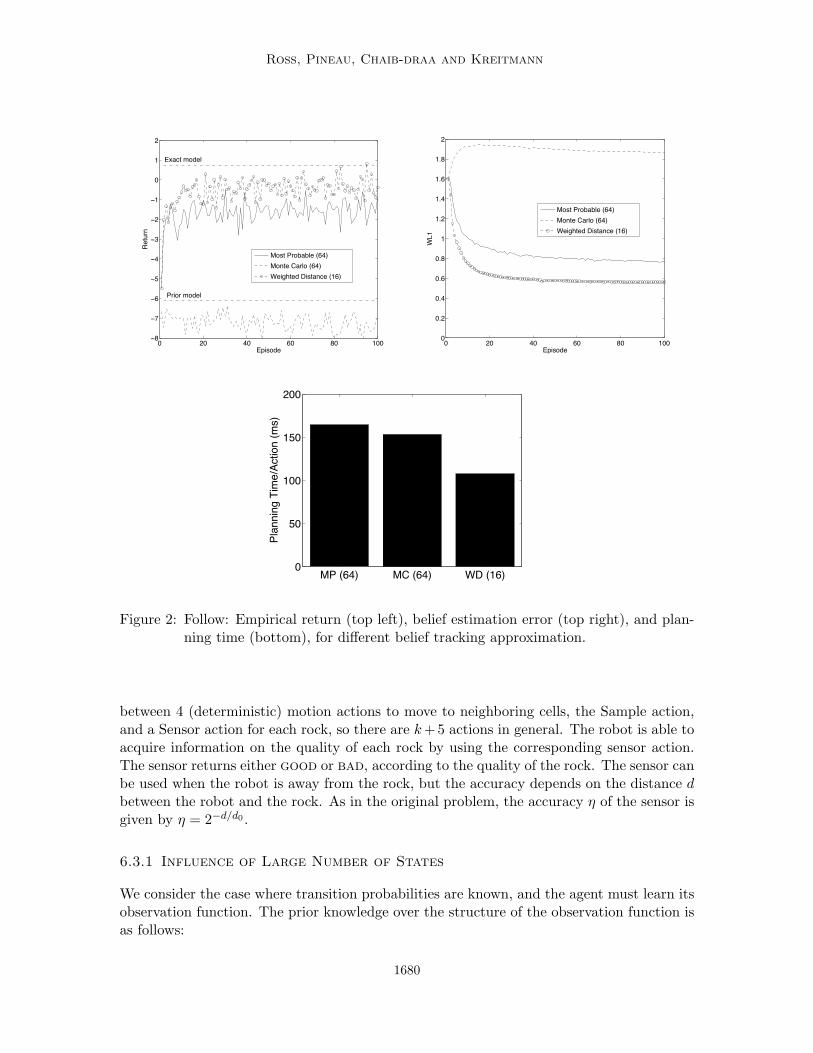
Figure 2 shows how the average return and model accuracy evolve over the 100 episodes(averaged over the 200 simulations) with different belief approximations. Figure 2 alsocompares the planning time taken by each approach. We observe from these figures that theresults for the Weighted Distance approximations are much better both in terms of returnand model accuracy, even with fewer particles (16). Monte-Carlo fails at providing anyimprovement over the prior model, which indicates it would require much more particles.Running Weighted Distance with 16 particles require less time than both Monte-Carloand Most Probable with 64 particles, showing that it can be more time efficient for theperformance it provides in complex environment.
6.3 RockSample
To test our algorithm against problems with a larger number of states, we consider theRockSample problem (Smith and Simmons, 2004). In this domain, a robot is on an n × nsquare board, with rocks on some of the cells. Each rock has an unknown binary quality(good or bad). The goal of the robot is to gather samples of the good rocks. Sampling agood rock yields high reward (+10), in contrast to sampling a bad rock (-10). However asample can only be acquired when the robot is in the same cell as the rock. The numberof rocks and their respective positions are fixed and known, while their qualities are fixedbut unknown. A state is defined by the position of the robot on the board and the qualityof all the rocks. With an n × n board and k rocks, the number of states is then n22k.Most results below assume n = 3 and k = 2, which makes 36 states. The robot can choose
1679
Ross, Pineau, Chaib-draa and Kreitmann
0 20 40 60 80 100−8
−7
−6
−5
−4
−3
−2
−1
0
1
2
Episode
Ret
urn
Most Probable (64)Monte Carlo (64)Weighted Distance (16)
Exact model
Prior model
0 20 40 60 80 1000
0.2
0.4
0.6
0.8
1
1.2
1.4
1.6
1.8
2
Episode
WL1
Most Probable (64)Monte Carlo (64)Weighted Distance (16)
MP (64) MC (64) WD (16)0
50
100
150
200
Plan
ning
Tim
e/Ac
tion
(ms)
Figure 2: Follow: Empirical return (top left), belief estimation error (top right), and plan-ning time (bottom), for different belief tracking approximation.
between 4 (deterministic) motion actions to move to neighboring cells, the Sample action,and a Sensor action for each rock, so there are k+ 5 actions in general. The robot is able toacquire information on the quality of each rock by using the corresponding sensor action.The sensor returns either good or bad, according to the quality of the rock. The sensor canbe used when the robot is away from the rock, but the accuracy depends on the distance dbetween the robot and the rock. As in the original problem, the accuracy η of the sensor isgiven by η = 2−d/d0 .
6.3.1 Influence of Large Number of States
We consider the case where transition probabilities are known, and the agent must learn itsobservation function. The prior knowledge over the structure of the observation function isas follows:
1680
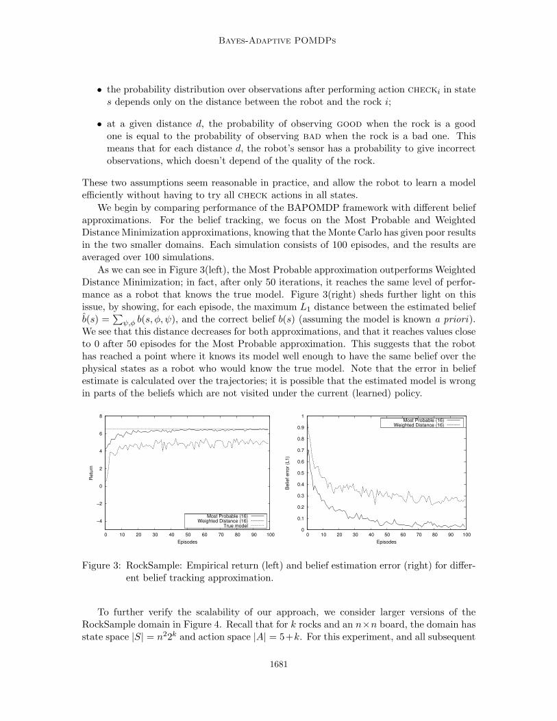
Bayes-Adaptive POMDPs
• the probability distribution over observations after performing action checki in states depends only on the distance between the robot and the rock i;
• at a given distance d, the probability of observing good when the rock is a goodone is equal to the probability of observing bad when the rock is a bad one. Thismeans that for each distance d, the robot’s sensor has a probability to give incorrectobservations, which doesn’t depend of the quality of the rock.
These two assumptions seem reasonable in practice, and allow the robot to learn a modelefficiently without having to try all check actions in all states.
We begin by comparing performance of the BAPOMDP framework with different beliefapproximations. For the belief tracking, we focus on the Most Probable and WeightedDistance Minimization approximations, knowing that the Monte Carlo has given poor resultsin the two smaller domains. Each simulation consists of 100 episodes, and the results areaveraged over 100 simulations.
As we can see in Figure 3(left), the Most Probable approximation outperforms WeightedDistance Minimization; in fact, after only 50 iterations, it reaches the same level of perfor-mance as a robot that knows the true model. Figure 3(right) sheds further light on thisissue, by showing, for each episode, the maximum L1 distance between the estimated beliefb(s) =
∑ψ,φ b(s, φ, ψ), and the correct belief b(s) (assuming the model is known a priori).
We see that this distance decreases for both approximations, and that it reaches values closeto 0 after 50 episodes for the Most Probable approximation. This suggests that the robothas reached a point where it knows its model well enough to have the same belief over thephysical states as a robot who would know the true model. Note that the error in beliefestimate is calculated over the trajectories; it is possible that the estimated model is wrongin parts of the beliefs which are not visited under the current (learned) policy.
−4
−2
0
2
4
6
8
0 10 20 30 40 50 60 70 80 90 100
Re
turn
Episodes
Most Probable (16)Weighted Distance (16)
True model 0
0.1
0.2
0.3
0.4
0.5
0.6
0.7
0.8
0.9
1
0 10 20 30 40 50 60 70 80 90 100
Be
lief
err
or
(L1
)
Episodes
Most Probable (16)Weighted Distance (16)
Figure 3: RockSample: Empirical return (left) and belief estimation error (right) for differ-ent belief tracking approximation.
To further verify the scalability of our approach, we consider larger versions of theRockSample domain in Figure 4. Recall that for k rocks and an n×n board, the domain hasstate space |S| = n22k and action space |A| = 5+k. For this experiment, and all subsequent
1681

Ross, Pineau, Chaib-draa and Kreitmann
ones, belief tracking in the BAPOMDP is done with the Most Probable approximation (withK = 16). As expected, the computational time for planning grows quickly with n and k.Better solutions could likely be obtained with appropriate use of heuristics in the forwardsearch planner (Ross et al., 2008c).
0.1
1
10
100
1000
10000
1 1.5 2 2.5 3 3.5 4 4.5 5
Tim
e,
in s
eco
nd
s
n
k = 1k = 2k = 3k = 4
Figure 4: RockSample: Computational time for different values of k and n. All results arecomputed with K = 16 and a depth=3 planning horizon.
6.3.2 Influence of the Priors
The choice of prior plays an important role in Bayesian Learning. As explained above, inthe RockSample domain we have constrained the structure of the observation probabilitymodel structural assumptions in the prior. For all results presented above, we used a priormade of 4 φ-vectors with probability 1
4 each. Each of those vectors φi is made of coefficients(φij), where φij is the probability that the sensor will give a correct observation at distancej. For each of the 4 vectors φi, we sample the coefficients φij from an uniform distributionbetween 0.45 and 0.95. We adopt this approach for a number of reasons. First, this prioris very general, in assuming that the sensor’s probability to make a mistake is uniformlydistributed between 0.05 and 0.55, at every distance d. Second, by sampling a new prior forevery simulation, we ensure that the results do not depend closely on inadvertent similaritiesbetween our prior and the correct model.
We now consider two other forms of prior. First, we consider the case where the coef-ficients φij are not sampled uniformly from U[0.45,0.95], but rather from U[φ∗j±ε], where φ∗j isthe value of the true model (that is, the probability that the true sensor gives a true ob-servation at distance j). We consider performance for various levels of noise, 0 ≤ ε ≤ 0.25.This experiment allows us to measure the influence of prior uncertainty on the performancesof our algorithm. The results in Figure 5 show that the BAPOMDP agent performs wellfor various levels of initial uncertainty over the model. As expected, the fact that all thepriors have φij coefficients centered around the true value φ∗j carries in itself substantialinformation, in many cases enough for the robot to perform very well from the first episode(note that the y-axis in Fig. 5 is different than that in Fig. 3). Furthermore, we observe
1682
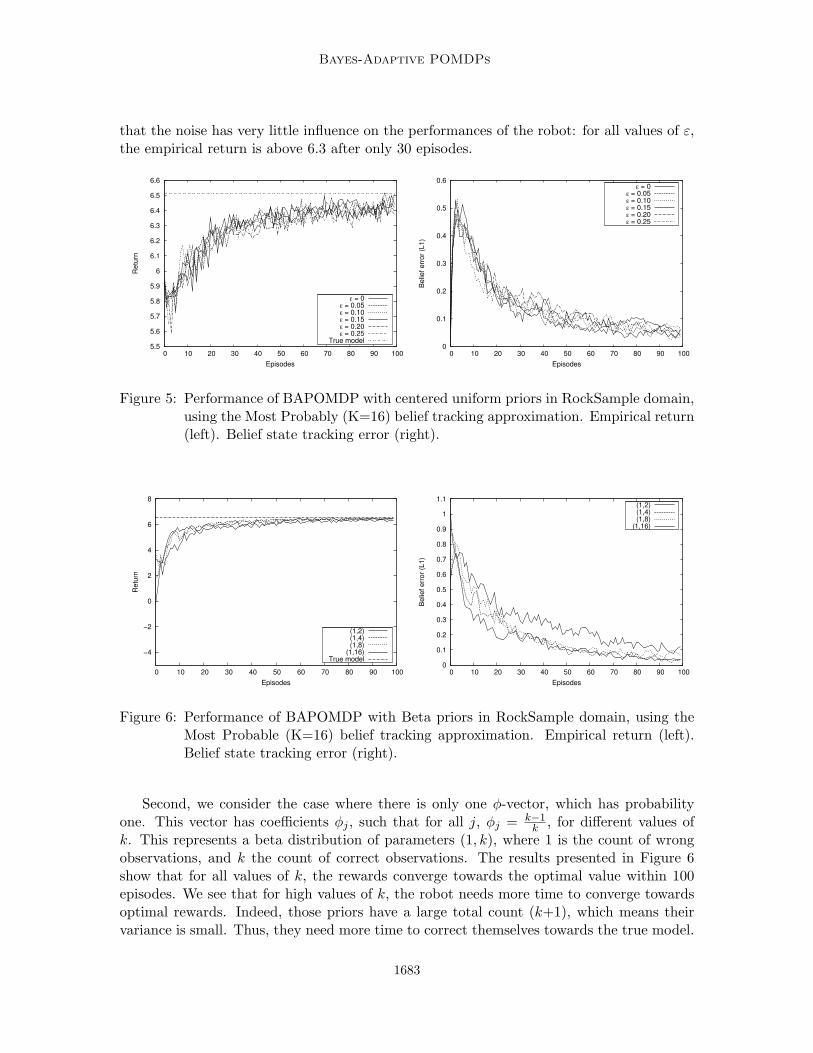
Bayes-Adaptive POMDPs
that the noise has very little influence on the performances of the robot: for all values of ε,the empirical return is above 6.3 after only 30 episodes.
5.5
5.6
5.7
5.8
5.9
6
6.1
6.2
6.3
6.4
6.5
6.6
0 10 20 30 40 50 60 70 80 90 100
Re
turn
Episodes
ε = 0ε = 0.05ε = 0.10ε = 0.15ε = 0.20ε = 0.25
True model 0
0.1
0.2
0.3
0.4
0.5
0.6
0 10 20 30 40 50 60 70 80 90 100
Be
lief
err
or
(L1
)
Episodes
ε = 0ε = 0.05ε = 0.10ε = 0.15ε = 0.20ε = 0.25
Figure 5: Performance of BAPOMDP with centered uniform priors in RockSample domain,using the Most Probably (K=16) belief tracking approximation. Empirical return(left). Belief state tracking error (right).
−4
−2
0
2
4
6
8
0 10 20 30 40 50 60 70 80 90 100
Re
turn
Episodes
(1,2)(1,4)(1,8)
(1,16)True model
0
0.1
0.2
0.3
0.4
0.5
0.6
0.7
0.8
0.9
1
1.1
0 10 20 30 40 50 60 70 80 90 100
Be
lief
err
or
(L1
)
Episodes
(1,2)(1,4)(1,8)
(1,16)
Figure 6: Performance of BAPOMDP with Beta priors in RockSample domain, using theMost Probable (K=16) belief tracking approximation. Empirical return (left).Belief state tracking error (right).
Second, we consider the case where there is only one φ-vector, which has probabilityone. This vector has coefficients φj , such that for all j, φj = k−1
k , for different values ofk. This represents a beta distribution of parameters (1, k), where 1 is the count of wrongobservations, and k the count of correct observations. The results presented in Figure 6show that for all values of k, the rewards converge towards the optimal value within 100episodes. We see that for high values of k, the robot needs more time to converge towardsoptimal rewards. Indeed, those priors have a large total count (k+1), which means theirvariance is small. Thus, they need more time to correct themselves towards the true model.
1683
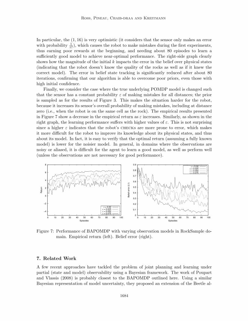
Ross, Pineau, Chaib-draa and Kreitmann
In particular, the (1, 16) is very optimistic (it considers that the sensor only makes an errorwith probability 1
17), which causes the robot to make mistakes during the first experiments,thus earning poor rewards at the beginning, and needing about 80 episodes to learn asufficiently good model to achieve near-optimal performance. The right-side graph clearlyshows how the magnitude of the initial k impacts the error in the belief over physical states(indicating that the robot doesn’t know the quality of the rocks as well as if it knew thecorrect model). The error in belief state tracking is significantly reduced after about 80iterations, confirming that our algorithm is able to overcome poor priors, even those withhigh initial confidence.
Finally, we consider the case where the true underlying POMDP model is changed suchthat the sensor has a constant probability ε of making mistakes for all distances; the prioris sampled as for the results of Figure 3. This makes the situation harder for the robot,because it increases its sensor’s overall probability of making mistakes, including at distancezero (i.e., when the robot is on the same cell as the rock). The empirical results presentedin Figure 7 show a decrease in the empirical return as ε increases. Similarly, as shown in theright graph, the learning performance suffers with higher values of ε. This is not surprisingsince a higher ε indicates that the robot’s checks are more prone to error, which makesit more difficult for the robot to improve its knowledge about its physical states, and thusabout its model. In fact, it is easy to verify that the optimal return (assuming a fully knownmodel) is lower for the noisier model. In general, in domains where the observations arenoisy or aliased, it is difficult for the agent to learn a good model, as well as perform well(unless the observations are not necessary for good performance).
−4
−2
0
2
4
6
8
0 10 20 30 40 50 60 70 80 90 100
Re
turn
Episodes
ε = 0.00ε = 0.025ε = 0.050ε = 0.075
0
0.1
0.2
0.3
0.4
0.5
0.6
0.7
0.8
0.9
0 10 20 30 40 50 60 70 80 90 100
Be
lief
err
or
(L1
)
Episodes
ε = 0.00ε = 0.025ε = 0.050ε = 0.075
Figure 7: Performance of BAPOMDP with varying observation models in RockSample do-main. Empirical return (left). Belief error (right).
7. Related Work
A few recent approaches have tackled the problem of joint planning and learning underpartial (state and model) observability using a Bayesian framework. The work of Poupartand Vlassis (2008) is probably closest to the BAPOMDP outlined here. Using a similarBayesian representation of model uncertainty, they proposed an extension of the Beetle al-
1684

Bayes-Adaptive POMDPs
gorithm (Poupart et al., 2006) (original designed for fully observable domains) to computean approximate solution for BAPOMDP-type problems. Their work is presented in thecontext of factored representations, but the model learning is done using similar Bayesianmechanisms, namely by updating a posterior represented by a mixture of Dirichlet distri-butions. They outline approximation methods to maintain a compact belief set that aresimilar to the Most Probably and Monte-Carlo methods outlined in Section 5.1 above. Pre-sumably our Weighted Distance minimization technique could be extended to their factoredrepresentation, assuming one can compute the distance metric. Finally, they propose anoffline planning algorithm, similar to the literature on point-based POMDP solvers, to finda policy. However we are not aware of any empirical validation with this approach, thusscalability and expressivity in experimental domains remains to be determined.
Jaulmes et al. (2005) have for their part considered active learning in partially observ-able domains where information gathering actions are provided by oracles that reveal theunderlying state. The key assumption of this approach, which is not used in other model-free approaches, concerns the existence of this oracle (or human) which is able to correctlyidentify the state following each transition. This makes it much easier to know how to up-date the prior. In the same vein than Jaulmes and colleagues, Doshi et al. (2008) developedan approach for active learning in POMDPs that can robustly determine a near-optimalpolicy. To achieve that, they introduced meta-queries (questions about action) and a risk-averse action selection criterion that allows agents to behave robustly even with uncertainknowledge of the POMDP model. Finally, Doshi-Velez (2010) proposed a Bayesian learn-ing framework for the case of POMDPs where the number of states is not known a priori,thus allowing the number of states to grow gradually as the agent explores the world, whilesimultaneously updating a posterior over the parameters.
The work on Universal Artificial Intelligence (Hutter, 2005) presents an interesting al-ternative to the framework of BAPOMDPs. It tackles a similar problem, namely sequentialdecision-making under (general) uncertainty. But Hutter’s AIXI framework is more general,in that it allows the model to be sampled from any computable distribution. The learningproblem is constrained by placing an Occam’s razor prior (measured by Kolmogorov com-plexity) over the space of models. The main drawback is that inference in this frameworkis incomputable, though an algorithm is presented for computing time/space-bounded solu-tions. Further development of a general purpose AIXI learning/planning algorithm wouldbe necessary to allow a direct comparison between AIXI and BAPOMDPs on practicalproblems. Recent results in Monte-Carlo Planning provide a good basis for this (Silver andVeness, 2010; Veness et al., 2011).
A number of useful theoretical results have also been published recently. For the specificcase of exploration in reinforcement learning, Asmuth et al. (2009) presented a fully Bayesiananalysis of the performance of a sampling approach. Subsequently, Kolter and Ng (2009)clarified the relation between Bayesian and PAC-MDP approaches and presented a simplealgorithm for efficiently achieving near-Bayesian exploration.
Finally, it is worth emphasizing that Bayesian approaches have also been investigated inthe control literature. The problem of optimal control under uncertain model parameterswas originally introduced by Feldbaum (1961), as the theory of dual control, also sometimesreferred to as adaptive dual control. Extensions of this theory have been developed for time-varying systems (Filatov and Unbehauen, 2000). Several authors have studied this problem
1685

Ross, Pineau, Chaib-draa and Kreitmann
for different kinds of dynamical systems : linear time invariant systems under partial ob-servability (Rusnak, 1995), linear time varying Gaussian models under partial observability(Ravikanth et al., 1992), nonlinear systems with full observability (Zane, 1992), and morerecently a non linear systems under partial observability (Greenfield and Brockwell, 2003).All this work is targeted towards specific classes of continuous systems, and we are notaware of similar work in the control literature for discrete (or hybrid) systems.
8. Conclusion
The problem of sequential decision-making under model uncertainty arises in many prac-tical applications of AI and decision systems. Developing effective models and algorithmsto handle these problems under realistic conditions—including stochasticity, partial stateobservability, and model inaccuracy—is imperative if we hope to deploy robots and otherautonomous agents in real-world situations.
This paper focuses in particular on the problem of simultaneous learning and decision-making in dynamic environments under partial model and state uncertainty. We adopt amodel-based Bayesian reinforcement learning framework, which allows us to explicitly targetthe exploration-exploitation problem in a coherent mathematical framework. Our work is adirect extension of previous results on model-based Bayesian reinforcement learning in fullyobservable domains.
The main contributions of the paper pertains to the development of the Bayes-AdaptivePOMDP model, and analysis of its theoretical properties. This work addresses a numberof interesting questions, including:
1. defining an appropriate model for POMDP parameter uncertainty,
2. approximating this model while maintaining performance guarantees,
3. performing tractable belief updating, and
4. optimizing action sequences given a posterior over state and model uncertainty.
From the theoretical analysis, we are able to derive simple algorithms for belief trackingand (near-)optimal decision-making in this model. We illustrate performance of these algo-rithms in a collection of synthetic POMDP domains. Results in the Follow problem showedthat our approach is able to learn the motion patterns of two (simulated) individuals. Thissuggests interesting applications in human-robot interaction, where we often lack good mod-els of human behavior and where it is imperative that an agent be able to learn quickly,lest the human user lose interest (this is in contrast to robot navigation tasks, for which weoften have access to more precise dynamical models and/or high-fidelity simulators). Fortheir part, results of RockSample problem shows how one should take into account priorknowledge on agent’s sensors when this knowledge is available.
While the BAPOMDP model provides a rich model for sequential decision-making underuncertainty, it has a number of important limitations. First, the model and theoreticalanalysis are limited to discrete domains. It is worth noting however that the approximatealgorithms extend quite easily to the continuous case (Ross et al., 2008b), at least for some
1686
Bayes-Adaptive POMDPs
families of dynamical systems. Other related references for the continuous case are availablein the control literature, as described in Section 7.
Another limitation is the fact that the model requires specification of a prior. Thisis standard in the Bayesian RL framework. The main concern is to ensure that the priorassigns some weight to the correct model. Our empirical evaluation shows good performancefor a range of priors; though the issue of choosing good priors in large domains remainsa challenge in general. Our empirical results also confirm standard Bayesian intuition,whereby the influence of the prior is particularly important for any inference and decision-making performed when only a small amount of data has been observed, but the influencebecomes negligible as large amounts of data are acquired.
As a word of caution, problems may arise in cases where Bayesian RL is used to inferboth transition and observation probabilities simultaneously, while the rewards are notexplicitly perceived through the observations (even if the rewards are known a priori). Inthis challenging setting, the Bayes-Adaptive POMDP framework as outlined above mightconverge to an incorrect model if the initial priors on the transition and observation modelare non-informative. This is mainly due to the fact that many possible parameters maycorrectly explain the observed action-observation sequences. While the agent is able topredict observations correctly, this leads to poor prediction of rewards and thus possibly sub-optimal long-term rewards. However if the rewards are observable, and their probabilitiestaken into account in the belief update, such problems do not arise, in the sense that theagent learns an equivalent model that correctly explains the observed action-observation-reward sequence and recovers a good policy for the unknown POMDP model. In the lattercase, where rewards are observable, the framework presented in this paper can be used withonly minor modifications to also learn the reward function.
Finally, it is worth pointing out that Bayesian RL methods in general have not beendeployed in real-world domains yet. We hope that the work presented here will motivatefurther investigation of practical issues pertaining to the application and deployment of thisclass of learning approaches.
Acknowledgments
This research was supported by the Natural Sciences and Engineering Research Council ofCanada (NSERC), the Fonds Quebecois de la Recherche sur la Nature et les Technologies(FQRNT), and the National Institutes of Health (grant R21DA019800). We would alsolike to thank Michael Bowling, Patrick Dallaire, Mohammad Ghavamzadeh, Doina Precup,Prakash Panangaden, as well as the anonymous reviewers, for offering thoughtful commentson earlier versions of this work.
Appendix A. Theorems and Proofs
This appendix presents the proofs of the theorems presented throughout this paper. The-orems 1 and 2 are presented first, then some useful lemmas, followed by the proofs of theremaining Theorems.
1687

Ross, Pineau, Chaib-draa and Kreitmann
Theorem 1 Let (S′, A, Z, T ′, O′, R′, γ) be a BAPOMDP constructed from the POMDP(S,A,Z, T,O,R, γ). If S is finite, then at any time t, the set S′b′t = {σ ∈ S′|b′t(σ) > 0} hassize |S′b′t | ≤ |S|
t+1.
Proof Proof by induction. When t = 0, b′0(s, φ, ψ) > 0 only if φ = φ0 and ψ = ψ0. Hence|S′b′0 | ≤ |S|. For the general case, assume that |S′b′t−1
| ≤ |S|t. From the definitions of thebelief update function, b′t(s
′, φ′, ψ′) > 0 iff ∃(s, φ, ψ) such that b′t−1(s, φ, ψ) > 0, φ′ = φ+δass′and ψ′ = ψ + δas′z. Hence, a particular (s, φ, ψ) such that b′t−1(s, φ, ψ) > 0 yields non-zeroprobabilities to at most |S| different states in b′t. Since |S′b′t−1
| ≤ |S|t by assumption, thenif we generate |S| different probable states in b′t, for each probable state in S′bt−1
it followsthat |S′b′t | ≤ |S|
t+1.
Theorem 2 For any horizon t, there exists a finite set Γt of functions S′ → R, such thatV ∗t (b) = maxα∈Γt
∑σ∈S′ α(σ)b(σ).
Proof Proof by induction. This holds true for horizon t = 1, since V ∗1 (b) =maxa∈A
∑(s,φ,ψ) b(s, φ, ψ)R(s, a). Hence by defining Γ1 = {αa|αa(s, φ, ψ) = R(s, a), a ∈ A},
V ∗1 (b) = maxα∈Γ1
∑σ∈S′ b(σ)α(σ). By induction, we assume that there exists a set Γt such
that V ∗t (b) = maxα∈Γt
∑σ∈S′ b(σ)α(σ).
Now V ∗t+1(b) = maxa∈A[∑
(s,φ,ψ) b(s, φ, ψ)R(s, a) +∑
z∈Z Pr(z|b, a)V ∗t (baz)]. Hence:
V ∗t+1(b) = maxa∈A[∑
(s,φ,ψ) b(s, φ, ψ)R(s, a) +∑
z∈Z Pr(z|b, a) maxα∈Γt
∑σ∈S′ b
az(σ)α(σ)]
= maxa∈A[∑
(s,φ,ψ) b(s, φ, ψ)R(s, a) +∑
z∈Z maxα∈Γt
∑σ∈S′ Pr(z|b, a)baz(σ)α(σ)
]= maxa∈A
[∑(s,φ,ψ) b(s, φ, ψ)R(s, a)+∑
z∈Z maxα∈Γt
∑(s,φ,ψ)∈S′
∑s′∈S b(s, φ, ψ)T sas
′φ Os
′azψ α(s′,U(φ, s, a, s′),U(ψ, s′, a, z))
].
Thus if we define:
Γt+1 = {αa,f |αa,f (s, φ, ψ) = R(s, a)+∑z∈Z
∑s′∈S T
sas′φ Os
′azψ f(z)(s′,U(φ, s, a, s′),U(ψ, s′, a, z)), a ∈ A, f ∈ [Z → Γt]},
then V ∗t+1(b) = maxα∈Γt+1
∑σ∈S′ b(σ)α(σ) and Γt+1 is finite since |Γt+1| = |A||Γt||Z|, which
is finite by assumptions that A, Z and Γt are all finite.
For some of the following theorems, lemmas and proofs, we will sometime denote theDirichlet count update operator U , as defined for the BAPOMDP, as a vector addition:φ′ = φ + δass′ = U(φ, s, a, s′), that is, δass′ is a vector full of zeros, with a 1 for the elementφass′ .
Lemma 1 For any t ≥ 2, any α-vector αt ∈ Γt can be expressed as αa,α′
t (s, φ, ψ) = R(s, a)+γ∑
z∈Z∑
s∈S′ Tsas′φ Os
′azψ α′(z)(s′, φ+δass′ , ψ+δas′z) for some a ∈ A, and α′ defining a mapping
Z → Γt−1.
1688

Bayes-Adaptive POMDPs
Proof Follows from proof of theorem 2.
Lemma 2 Given any a, b, c, d ∈ R, ab− cd = (a−c)(b+d)+(a+c)(b−d)2 .
Proof Follows from direct computation.
Lemma 3 Given any φ, φ′ ∈ T , ψ,ψ′ ∈ O, then for all s ∈ S, a ∈ A, we have that∑s′∈S
∑z∈Z
∣∣∣∣ φ′ass′ψ′as′zN saφ′ N
s′aψ′− φa
ss′ψas′z
N saφ Ns′aψ
∣∣∣∣ ≤ DsaS (φ′, φ) + sups′∈S Ds′a
Z (ψ′, ψ).
Proof Using lemma 2, we have that:∑s′∈S
∑z∈Z
∣∣∣∣ φ′ass′ψ′as′zN saφ′ N
s′aψ′− φa
ss′ψas′z
N saφ Ns′aψ
∣∣∣∣= 1
2
∑s′∈S
∑z∈Z
∣∣∣∣( φ′ass′N saφ′− φa
ss′N saφ
)(ψ′as′zN s′aψ′
+ψas′zN s′aψ
)+(φ′ass′N saφ′
+φass′N saφ
)(ψ′as′zN s′aψ′− ψa
s′zN s′aψ
)∣∣∣∣≤ 1
2
∑s′∈S
∣∣∣∣ φ′ass′N saφ′− φa
ss′N saφ
∣∣∣∣∑z∈Z
∣∣∣∣ ψ′as′zN s′aψ′
+ψas′zN s′aψ
∣∣∣∣+ 12
∑s′∈S
∣∣∣∣ φ′ass′N saφ′
+φass′N saφ
∣∣∣∣∑z∈Z
∣∣∣∣ ψ′as′zN s′aψ′− ψa
s′zN s′aψ
∣∣∣∣≤
∑s′∈S
∣∣∣∣ φ′ass′N saφ′− φa
ss′N saφ
∣∣∣∣+ 12
[sups′∈S
∑z∈Z
∣∣∣∣ ψ′as′zN s′aψ′− ψa
s′zN s′aψ
∣∣∣∣] [∑s′∈S
∣∣∣∣ φ′ass′N saφ′
+φass′N saφ
∣∣∣∣]=
∑s′∈S
∣∣∣∣ φ′ass′N saφ′− φa
ss′N saφ
∣∣∣∣+ sups′∈S∑
z∈Z
∣∣∣∣ ψ′as′zN s′aψ′− ψa
s′zN s′aψ
∣∣∣∣= Dsa
S (φ′, φ) + sups′∈S Ds′aZ (ψ′, ψ).
Lemma 4 Given any φ, φ′,∆ ∈ T , then for all s ∈ S, a ∈ A,DsaS (φ+ ∆, φ′ + ∆) ≤ Dsa
S (φ, φ′) +2N sa∆
Ps′∈S |φass′−φ
′ass′ |
(N saφ +N sa∆ )(N saφ′ +N sa∆ ) .
Proof We have that:
DsaS (φ+ ∆, φ′ + ∆)
=∑
s′∈S
∣∣∣∣φass′+∆ass′
N saφ +N sa∆− φ′a
ss′+∆ass′
N saφ′ +N sa∆
∣∣∣∣=
∑s′∈S
∣∣∣∣ (φass′+∆ass′ )(N
saφ′ +N sa∆ )−(φ′a
ss′+∆ass′ )(N
saφ +N sa∆ )
(N saφ +N sa∆ )(N saφ′ +N sa∆ )
∣∣∣∣=
∑s′∈S
∣∣∣∣φass′N saφ′ +φass′N
sa∆ +∆a
ss′Nsaφ′ −φ
′ass′N
saφ −φ
′ass′N
sa∆ −∆a
ss′Nsaφ
(N saφ +N sa∆ )(N saφ′ +N sa∆ )
∣∣∣∣≤
∑s′∈S
∣∣∣∣ φass′N
saφ′ −φ
′ass′N
saφ
(N saφ +N sa∆ )(N saφ′ +N sa∆ )
∣∣∣∣+∑
s′∈S
∣∣∣∣N sa∆ (φass′−φ
′ass′ )+∆a
ss′ (Nsaφ′ −N
saφ )
(N saφ +N sa∆ )(N saφ′ +N sa∆ )
∣∣∣∣≤
∑s′∈S
∣∣∣∣φass′N saφ′ −φ′ass′N saφN saφ Nsaφ′
∣∣∣∣+N sa∆ [
Ps′∈S|φass′−φ′ass′ |]+
˛N saφ′ −N
saφ
˛Ps′∈S ∆a
ss′
(N saφ +N sa∆ )(N saφ′ +N sa∆ )
= DsaS (φ, φ′) +
N sa∆ [Ps′∈S|φass′−φ′ass′ |]+N sa∆
˛N saφ′ −N
saφ
˛(N saφ +N sa∆ )(N sa
φ′ +N sa∆ )
≤ DsaS (φ, φ′) +
2N sa∆
Ps′∈S|φass′−φ′ass′ |
(N saφ +N sa∆ )(N saφ′ +N sa∆ ) .
1689

Ross, Pineau, Chaib-draa and Kreitmann
Lemma 5 Given any ψ,ψ′,∆ ∈ O, then for all s ∈ S, a ∈ A,DsaZ (ψ + ∆, ψ′ + ∆) ≤ Dsa
Z (ψ,ψ′) + 2N sa∆
Pz∈Z |ψasz−ψ′asz |
(N saψ +N sa∆ )(N saψ′+N
sa∆ ) .
Proof Same proof as for lemma 4, except that we sum over z ∈ Z in this case.
Lemma 6 Given any γ ∈ (0, 1), then supx γx/2x = 2ln(γ−e) .
Proof We observe that when x = 0, γx/2x = 0 and limx→∞ γx/2x = 0. Furthermore, γx/2
is monotonically decreasing exponentially as x increases, while x is monotonically increasinglinearly as x increases. Thus it is clear that γx/2x will have a unique global maximum in(0,∞). We can find this maximum by taking the derivative:
∂∂x(γx/2x)
= (ln γ)γx/2x2 + γx/2
= γx/2( (ln γ)x2 + 1).
Hence by solving when this is equal 0, we have:
γx/2( (ln γ)x2 + 1) = 0
⇔ (ln γ)x2 + 1 = 0
⇔ x = −2ln γ = −2 logγ(e).
Hence we have that:γx/2x
≤ −2γ− logγ(e) logγ(e)= −2e−1 logγ(e)= 2
ln(γ−e) .
Lemma 7 supα1∈Γ1,s∈S |α1(s, φ, ψ)− α1(s, φ′, ψ′)| = 0 for any φ, φ′, ψ, ψ′.
Proof For any a ∈ A, s ∈ S, |αa1(s, φ, ψ)− αa1(s, φ′, ψ′)| = |R(s, a)−R(s, a)| = 0.
Theorem 3 Given any φ, φ′ ∈ T , ψ,ψ′ ∈ O and γ ∈ (0, 1), then ∀t:
supαt∈Γt,s∈S
|αt(s, φ, ψ)− αt(s, φ′, ψ′)| ≤ 2γ||R||∞(1−γ)2 sup
s,s′∈S,a∈A
[DsaS (φ, φ′) +Ds′a
Z (ψ,ψ′)+
4ln(γ−e)
(Ps′′∈S|φass′′−φ′ass′′ |
(N saφ +1)(N saφ′ +1) +
Pz∈Z |ψas′z−ψ′as′z|
(N s′aψ +1)(N s′aψ′ +1)
)].
1690

Bayes-Adaptive POMDPs
Proof Using lemma 1, we have that:
|αa,α′
t (s, φ, ψ)− αa,α′
t (s, φ′, ψ′)|
=∣∣∣∣R(s, a) + γ
∑s′∈S
∑z∈Z
φass′ψ
as′z
N saφ Ns′aψ
α′(z)(s′, φ+ δass′ , ψ + δas′z)
−R(s, a)− γ∑
s′∈S∑
z∈Zφ′ass′ψ
′as′z
N saφ′ N
s′aψ′α′(z)(s′, φ′ + δass′ , ψ
′ + δas′z)∣∣∣∣
= γ
∣∣∣∣∑s′∈S∑
z∈Z
[φass′ψ
as′z
N saφ Ns′aψ
α′(z)(s′, φ+ δass′ , ψ + δas′z)−φ′ass′ψ
′as′z
N saφ′ N
s′aψ′α′(z)(s′, φ′ + δass′ , ψ
′ + δas′z)]∣∣∣∣
= γ
∣∣∣∣∑s′∈S∑
z∈Z
[φass′ψ
as′z
N saφ Ns′aψ
(α′(z)(s′, φ+ δass′ , ψ + δas′z)− α′(z)(s′, φ′ + δass′ , ψ′ + δas′z))
−(
φ′ass′ψ
′as′z
N saφ′ N
s′aψ′− φa
ss′ψas′z
N saφ Ns′aψ
)α′(z)(s′, φ′ + δass′ , ψ
′ + δas′z)]∣∣∣∣
≤ γ∑
s′∈S∑
z∈Zφass′ψ
as′z
N saφ Ns′aψ
∣∣α′(z)(s′, φ+ δass′ , ψ + δas′z)− α′(z)(s′, φ′ + δass′ , ψ′ + δas′z)
∣∣+γ∑
s′∈S∑
z∈Z
∣∣∣∣ φ′ass′ψ′as′zN saφ′ N
s′aψ′− φa
ss′ψas′z
N saφ Ns′aψ
∣∣∣∣ ∣∣α′(z)(s′, φ′ + δass′ , ψ′ + δas′z)
∣∣≤ γ sup
s′∈S,z∈Z
∣∣α′(z)(s′, φ+ δass′ , ψ + δas′z)− α′(z)(s′, φ′ + δass′ , ψ′ + δas′z)
∣∣+γ||R||∞
1−γ∑
s′∈S∑
z∈Z
∣∣∣∣ φ′ass′ψ′as′zN saφ′ N
s′aψ′− φa
ss′ψas′z
N saφ Ns′aψ
∣∣∣∣≤ γ sup
s′∈S,z∈Z
∣∣α′(z)(s′, φ+ δass′ , ψ + δas′z)− α′(z)(s′, φ′ + δass′ , ψ′ + δas′z)
∣∣+γ||R||∞
1−γ
(DsaS (φ′, φ) + sups′∈S Ds′a
Z (ψ′, ψ)).
The last inequality follows from lemma 3. Hence by taking the sup we get:
supαt∈Γt,s∈S |αt(s, φ, ψ)− αt(s, φ′, ψ′)|≤ γ sup
s,s′∈S,a∈A,z∈Z,αt−1∈Γt−1
∣∣αt−1(s′, φ+ δass′ , ψ + δas′z)− αt−1(s′, φ′ + δass′ , ψ′ + δas′z)
∣∣+γ||R||∞
1−γ sups,s′∈S,a∈A
(DsaS (φ′, φ) +Ds′a
Z (ψ′, ψ)).
We notice that this inequality defines a recurrence. By unfolding it up to t = 1 we get that:
supαt∈Γt,s∈S |αt(s, φ, ψ)− αt(s, φ′, ψ′)|≤ γt−1 sup
α1∈Γ1,s′∈S,∆∈T ,∆′∈O| ||∆||1=||∆′||1=(t−1)|α1(s′, φ+ ∆, ψ + ∆′)− α1(s′, φ′ + ∆, ψ′ + ∆′)|
+γ||R||∞1−γ
∑t−2i=1 γ
i sups,s′∈S,a∈A,∆∈T ,∆′∈O| ||∆||1=||∆′||1=i
(DsaS (φ′ + ∆, φ+ ∆) +Ds′a
Z (ψ′ + ∆′, ψ + ∆′))
+γ||R||∞1−γ sup
s,s′∈S,a∈A
(DsaS (φ′, φ) +Ds′a
Z (ψ′, ψ)).
1691

Ross, Pineau, Chaib-draa and Kreitmann
Applying lemmas 7, 4 and 5 to the last term, we get that:
supαt∈Γt,s∈S |αt(s, φ, ψ)− αt(s, φ′, ψ′)|≤ γ||R||∞
1−γ∑t−2
i=1 γi sups,s′∈S,a∈A,∆∈T ,∆′∈O| ||∆||1=||∆′||1=i
(DsaS (φ′, φ) +Ds′a
Z (ψ′, ψ)
+2N sa∆
Ps′′∈S |φass′′−φ
′ass′′ |
(N saφ +N sa∆ )(N saφ′ +N sa∆ ) +
2N s′a∆′Pz∈Z |ψas′z−ψ
′as′z |
(N s′aψ +N s′a∆′ )(N s′a
ψ′ +N s′a∆′ )
)+γ||R||∞
1−γ sups,s′∈S,a∈A
(DsaS (φ′, φ) +Ds′a
Z (ψ′, ψ))
= γ||R||∞1−γ
∑t−2i=1 γ
i/2 sups,s′∈S,a∈A,∆∈T ,∆′∈O| ||∆||1=||∆′||1=i
(γi/2Dsa
S (φ′, φ) + γi/2Ds′aZ (ψ′, ψ)
+2γi/2N sa∆
Ps′′∈S |φass′′−φ
′ass′′ |
(N saφ +N sa∆ )(N saφ′ +N sa∆ ) +
2γi/2N s′a∆′Pz∈Z |ψas′z−ψ
′as′z |
(N s′aψ +N s′a∆′ )(N s′a
ψ′ +N s′a∆′ )
)+γ||R||∞
1−γ sups,s′∈S,a∈A
(DsaS (φ′, φ) +Ds′a
Z (ψ′, ψ)).
Now we notice that γi/2 ≤ γNsa∆ /2 since ||∆||1 = i, and similarly γi/2 ≤ γN
sa∆′/2. Hence by
applying lemma 6, we get that:
supαt∈Γt,s∈S |αt(s, φ, ψ)− αt(s, φ′, ψ′)|≤ γ||R||∞
1−γ∑t−2
i=1 γi/2 sup
s,s′∈S,a∈A,∆∈T ,∆′∈O| ||∆||1=||∆′||1=i
(DsaS (φ′, φ) +Ds′a
Z (ψ′, ψ)
+4Ps′′∈S |φass′′−φ
′ass′′ |
ln(γ−e)(N saφ +N sa∆ )(N saφ′ +N sa∆ )
+4Pz∈Z |ψas′z−ψ
′as′z |
ln(γ−e)(N s′aψ +N s′a∆′ )(N s′a
ψ′ +N s′a∆′ )
)+γ||R||∞
1−γ sups,s′∈S,a∈A
(DsaS (φ′, φ) +Ds′a
Z (ψ′, ψ))
≤ γ||R||∞1−γ
∑t−2i=1 γ
i/2 sups,s′∈S,a∈A
(DsaS (φ′, φ) +Ds′a
Z (ψ′, ψ) +4Ps′′∈S |φass′′−φ
′ass′′ |
ln(γ−e)(N saφ +1)(N saφ′ +1)
+4Pz∈Z |ψas′z−ψ
′as′z |
ln(γ−e)(N s′aψ +1)(N s′aψ′ +1)
)+ γ||R||∞
1−γ sups,s′∈S,a∈A
(DsaS (φ′, φ) +Ds′a
Z (ψ′, ψ))
≤(∑t−2
i=0 γi/2)γ||R||∞
1−γ sups,s′∈S,a∈A
[DsaS (φ′, φ) +Ds′a
Z (ψ′, ψ)
+ 4ln(γ−e)
(Ps′′∈S |φass′′−φ
′ass′′ |
(N saφ +1)(N saφ′ +1) +
Pz∈Z |ψas′z−ψ
′as′z |
(N s′aψ +1)(N s′aψ′ +1)
)]≤
(∑∞i=0 γ
i/2) γ||R||∞
1−γ sups,s′∈S,a∈A
[DsaS (φ′, φ) +Ds′a
Z (ψ′, ψ)
+ 4ln(γ−e)
(Ps′′∈S |φass′′−φ
′ass′′ |
(N saφ +1)(N saφ′ +1) +
Pz∈Z |ψas′z−ψ
′as′z |
(N s′aψ +1)(N s′aψ′ +1)
)]= 1+
√γ
1−γγ||R||∞
1−γ sups,s′∈S,a∈A
[DsaS (φ′, φ) +Ds′a
Z (ψ′, ψ) + 4ln(γ−e)
(Ps′′∈S |φass′′−φ
′ass′′ |
(N saφ +1)(N saφ′ +1) +
Pz∈Z |ψas′z−ψ
′as′z |
(N s′aψ +1)(N s′aψ′ +1)
)]≤ 2γ||R||∞
(1−γ)2 sups,s′∈S,a∈A
[DsaS (φ′, φ) +Ds′a
Z (ψ′, ψ) + 4ln(γ−e)
(Ps′′∈S |φass′′−φ
′ass′′ |
(N saφ +1)(N saφ′ +1) +
Pz∈Z |ψas′z−ψ
′as′z |
(N s′aψ +1)(N s′aψ′ +1)
)].
Lemma 8 Given φ ∈ T , s ∈ S, a ∈ A, then for all ∆ ∈ T ,Ps′∈S |φass′−(φa
ss′+∆ass′ )|
(N saφ +1)(N saφ +N sa∆ +1) ≤1
N saφ +1 .
1692

Bayes-Adaptive POMDPs
Proof Ps′∈S |φass′−(φa
ss′+∆ass′ )|
(N saφ +1)(N saφ +N sa∆ +1)
=Ps′∈S ∆a
ss′(N saφ +1)(N saφ +N sa∆ +1)
= 1N saφ +1
(N sa∆
N sa∆ +N saφ +1
).
The term N sa∆N sa∆ +N saφ +1 is monotonically increasing and converge to 1 as N sa
∆ →∞. Thus thelemma follows.
Corollary 1 Given ε > 0, φ ∈ T , s ∈ S, a ∈ A, if N saφ > 1
ε −1 then for all ∆ ∈ T we have
thatPs′∈S |φass′−(φa
ss′+∆ass′ )|
(N saφ +1)(N saφ +N sa∆ +1) < ε.
Proof According to lemma 8, we know that for all ∆ ∈ T , we have thatPs′∈S |φass′−(φa
ss′+∆ass′ )|
(N saφ +1)(N saφ +N sa∆ +1) ≤1
N saφ +1 . Hence if N saφ > 1
ε − 1, then 1N saφ +1 < ε.
Lemma 9 Given ψ ∈ O, s ∈ S, a ∈ A, then for all ∆ ∈ O,Pz∈Z |ψasz−(ψasz+∆a
sz)|(N saψ +1)(N saψ +N sa∆ +1) ≤
1N saψ +1 .
Proof Same proof as lemma 8.
Corollary 2 Given ε > 0, ψ ∈ O, s ∈ S, a ∈ A, if N saψ > 1
ε − 1 then for all ∆ ∈ O we
have thatPz∈Z |ψasz−(ψasz+∆a
sz)|(N saψ +1)(N saψ +N sa∆ +1) < ε
Proof Same proof as corollary 1, but using lemma 9 instead.
Theorem 4 Given any ε > 0 and (s, φ, ψ) ∈ S′ such that ∃a ∈ A, ∃s′ ∈ S, N s′aφ > N ε
S orN s′aψ > N ε
Z , then ∃(s, φ′, ψ′) ∈ S′ such that ∀a ∈ A, ∀s′ ∈ S, N s′aφ′ ≤ N ε
S, N s′aψ′ ≤ N ε
Z and|αt(s, φ, ψ)− αt(s, φ′, ψ′)| < ε holds for all t and αt ∈ Γt.
Proof Consider an arbitrary ε > 0. We first find a bound on N saφ and N sa
ψ such that anyvector with higher counts is within ε distance of another vector with lower counts. Let’sdefine ε′ = ε(1−γ)2
8γ||R||∞ and ε′′ = ε(1−γ)2 ln(γ−e)32γ||R||∞ . According to corollary 1, we have that for any
φ ∈ T such that N saφ > 1
ε′′ − 1, then for all φ′ ∈ T such that there exists a ∆ ∈ T where
φ′ = φ+ ∆, thenPs′′∈S |φass′′−φ
′ass′′ |
(N saφ +1)(N saφ′ +1) < ε′′. Hence we want to find an N such that given φ ∈ T
with N saφ > N , there exists a φ′ ∈ T such that N sa
φ′ ≤ N , DsaS (φ, φ′) < ε′ and exists a ∆ ∈ T
such that φ = φ′ + ∆. Let’s consider an arbitrary φ such that N saφ > N . We can construct
a new vector φ′ as follows, for all s′ define φ′ass′ =⌊Nφa
ss′N saφ
⌋and for all other a′ 6= a, s′′ 6= s,
define φ′a′
s′′s′ = φa′s′′s′ for all s′. Clearly, φ′ ∈ T , such that N − |S| ≤ N sa
φ′ ≤ N . Moreover, wehave that φ′a
′s′s′′ ≤ φa
′s′s′′ for all s′, a′, s′′, and thus there exists a ∆ ∈ T such that φ = φ′+ ∆.
1693
Ross, Pineau, Chaib-draa and Kreitmann
Furthermore, from its construction, we know that ∀s′,∣∣∣∣ φ′ass′N sa
φ′− φa
ss′N saφ
∣∣∣∣ ≤ 1N saφ′
. Hence it is clear
from this that DsaS (φ, φ′) ≤ |S|
N−|S| . Thus, if we want DsaS (φ, φ′) < ε′, we just need to take
N > |S|(1+ε′)ε′ . Since we also want N > 1
ε′′ − 1, let’s just define NS = max(|S|(1+ε′)
ε′ , 1ε′′ − 1
).
NS = N εS , as defined in Section 4, will be our bound on N sa
φ such that, as we have justshowed, for any φ ∈ T such that N sa
φ > NS , we can find a φ′ ∈ T such that N saφ′ ≤ NS ,
DsaS (φ, φ′) < ε′ and
Ps′′∈S |φass′′−φ
′ass′′ |
(N saφ +1)(N saφ′ +1) < ε′′. Similarly, since we have a similar corollary
(corollary 1) for the observation counts ψ, we can proceed in the same way and defineNZ = max
(|Z|(1+ε′)
ε′ , 1ε′′ − 1
), such that for any ψ ∈ O such that N sa
ψ > NZ , we can find
a ψ′ ∈ O such that N saψ′ ≤ NZ , Dsa
Z (ψ,ψ′) < ε′ andPz∈Z |ψasz−ψ′asz |
(N saψ +1)(N saψ′+1) < ε′′. NZ = N ε
Z as we
have defined in Section 4.Now let S = {(s, φ, ψ) ∈ S′|∀s′ ∈ S, a ∈ A,N s′a
φ ≤ NS & N s′aψ ≤ NZ} and consider an arbi-
trary (s, φ, ψ) ∈ S′. For any s′ ∈ S, a ∈ A, such that N s′aφ > NS , there exists a φ′ ∈ T such
thatN s′aφ′ ≤ NS , Ds′a
S (φ, φ′) < ε′ andPs′′∈S |φas′s′′−φ
′as′s′′ |
(N s′aφ +1)(N s′aφ′ +1)
< ε′′ (as we have just showed above).
Thus let’s define φas′s′′ = φ′as′s′′ for all s′′ ∈ S. For any s′ ∈ S, a ∈ A, such that N s′aφ ≤ NS ,
just set φas′s′′ = φas′s′′ , ∀s′′ ∈ S. Similarly, for any s′ ∈ S, a ∈ A, such that N s′aψ > NZ ,
there exists a ψ′ ∈ O such that N s′aψ′ ≤ NZ , Ds′a
Z (ψ,ψ′) < ε′ andPz∈Z |ψas′z−ψ
′as′z |
(N s′aψ +1)(N s′aψ′ +1)
< ε′′ (as
we have just showed above). Thus let’s define ψas′s′′ = ψ′as′s′′ for all s′′ ∈ S. For any s′ ∈ S,a ∈ A, such that N s′a
ψ ≤ NZ , just set ψas′s′′ = ψas′s′′ ∀s′′ ∈ S. Now it is clear from this con-struction that (s, φ, ψ) ∈ S. By Theorem 3, for any t, supαt∈Γt,s∈S |αt(s, φ, ψ)−αt(s, φ, ψ)| ≤2γ||R||∞(1−γ)2 sup
s,s′∈S,a∈A
[Ds,aS (φ, φ) +Ds′,a
Z (ψ, ψ) + 4ln(γ−e)
(Ps′′∈S |φass′′−φ
ass′′ |
(N saφ +1)(N saφ
+1) +Pz∈Z |ψas′z−ψ
as′z |
(N s′aψ +1)(N s′aψ
+1)
)]<
2γ||R||∞(1−γ)2
[ε′ + ε′ + 4
ln(γ−e) (ε′′ + ε′′)]
= ε.
Theorem 5 Given any ε > 0, (s, φ, ψ) ∈ S′ and αt ∈ Γt computed from the infiniteBAPOMDP. Let αt be the α-vector representing the same conditional plan as αt but com-puted with the finite BAPOMDP (Sε, A, Z, Tε, Oε, Rε, γ), then |αt(Pε(s, φ, ψ))−αt(s, φ, ψ)| <ε
1−γ .
Proof Let (s, φ′, ψ′) = Pε(s, φ, ψ).
|αt(Pε(s, φ, ψ))− αt(s, φ, ψ)|≤ |αt(s, φ′, ψ′)− αt(s, φ′, ψ′)|+ |αt(s, φ′, ψ′)− αt(s, φ, ψ)|< |αt(s, φ′, ψ′)− αt(s, φ′, ψ′)|+ ε (by Theorem 4)= |γ
∑z∈Z
∑s′∈S T
sas′φ′ Os
′azψ′
[α′(z)(Pε(s′, φ′ + δass′ , ψ
′ + δas′z))− α′(z)(s′, φ′ + δass′ , ψ′ + δas′z)
]|+ ε
≤ γ∑
z∈Z∑
s′∈S Tsas′φ′ Os
′azψ′
∣∣α′(z)(Pε(s′, φ′ + δass′ , ψ′ + δas′z))− α′(z)(s′, φ′ + δass′ , ψ
′ + δas′z)∣∣+ ε
≤ γ supz∈Z,s′∈S∣∣α′(z)(Pε(s′, φ′ + δass′ , ψ
′ + δas′z))− α′(z)(s′, φ′ + δass′ , ψ′ + δas′z)
∣∣+ ε
≤ γ supαt−1∈Γt−1,(s′,φ′′,ψ′′)∈S′ |αt−1(Pε(s′, φ′′, ψ′′))− αt−1(s′, φ′′, ψ′′)|+ ε.
1694

Bayes-Adaptive POMDPs
Thus, we have that:
supαt∈Γt,σ∈S′ |αt(Pε(σ))− αt(σ)|< γ supαt−1∈Γt−1,σ′∈S′ |αt−1(Pε(σ′))− αt−1(σ′)|+ ε.
This defines a recurrence. By unfolding it up to t = 1, where ∀σ ∈ S′, α1(Pε(σ)) = α1(σ),we get that supαt∈Γt,σ∈S′ |αt(Pε(σ))−αt(σ)| < ε
∑t−2i=0 γ
i. Hence for all t, this is lower thanε
1−γ .
Theorem 6 Given any ε > 0, and any horizon t, let πt be the optimal t-step policy com-puted from the finite POMDP (Sε, A, Z, Tε, Oε, Rε, γ), then for any initial belief b the valueof executing policy πt in the BAPOMDP Vπt(b) ≥ V ∗(b)− 2 ε
1−γ .
Proof Pick any starting belief b in the BAPOMDP. Let α∗ denote the optimal t-stepcondition plan in the BAPOMDP for b: α∗ = argmaxα∈Γt
∑(s,φ,ψ) b(s, φ, ψ)α(s, φ, ψ), such
that the value of this optimal conditional plan is∑
(s,φ,ψ) b(s, φ, ψ)α∗(s, φ, ψ) = V ∗(b).Denote α∗ the corresponding α-vector representing the same t-step conditional plan in thefinite POMDP approximation.
Now let α′ = argmaxα∈Γt
∑(s,φ,ψ) b(s, φ, ψ)α(Pε(s, φ, ψ)) be the optimal t-step con-
ditional plan in the finite POMDP approximation if we start in belief b. This condi-tional plan represents exactly what the policy πt would do over t-steps starting in b.Denote α′ the corresponding α-function in the BAPOMDP representing the same t-stepconditional plan. Then the value of executing πt starting in b in the BAPOMDP isVπt(b) =
∑(s,φ,ψ) b(s, φ, ψ)α′(s, φ, ψ). Using Theorem 5, this value is lower bounded as
follows:
Vπt(b)=
∑(s,φ,ψ) b(s, φ, ψ)α′(s, φ, ψ)
≥∑
(s,φ,ψ) b(s, φ, ψ)α′(Pε(s, φ, ψ))− ε1−γ
≥∑
(s,φ,ψ) b(s, φ, ψ)α∗(Pε(s, φ, ψ))− ε1−γ
≥∑
(s,φ,ψ) b(s, φ, ψ)α∗(Pε(s, φ, ψ))− 2 ε1−γ
= V ∗(b)− 2 ε1−γ .
References
J. Asmuth, L. Li, M. Littman, A. Nouri, and D. Wingate. A bayesian sampling approachto exploration in reinforcement learning. In Conference on Uncertainty in Artificial In-telligence (UAI), 2009.
P. Auer and R. Ortner. Logarithmic online regret bounds for undiscounted reinforcementlearning. In Neural Information Processing Systems (NIPS), volume 19, pages 49–56,2006.
1695
Ross, Pineau, Chaib-draa and Kreitmann
P. Auer, T. Jaksch, and R. Ortner. Near-optimal regret bounds for reinforcement learning.In Neural Information Processing Systems (NIPS), volume 21, 2009.
J. Baxter and P. L. Bartlett. Infinite-horizon policy-gradient estimation. Journal of ArtificialIntelligence Research (JAIR), 15:319–350, 2001.
R. Bellman. Adaptive Control Processes: A Guided Tour. Princeton University Press, 1961.
R. I. Brafman and M. Tennenholtz. R-max - a general polynomial time algorithm fornear-optimal reinforcement learning. Journal of Machine Learning Research (JMLR), 3:213–231, 2003.
G. Casella and R. Berger. Statistical Inference. Duxbury Resource Center, 2001.
P. S. Castro and D. Precup. Using linear programming for bayesian exploration in markovdecision processes. In International Joint Conference on Artificial Intelligence (IJCAI),pages 2437–2442, 2007.
R. Dearden, N. Friedman, and S. J. Russell. Bayesian Q-learning. In AAAI Conference onArtificial Intelligence, pages 761–768, 1998.
R. Dearden, N. Friedman, and D. Andre. Model based bayesian exploration. In Conferenceon Uncertainty in Artificial Intelligence (UAI), pages 150–159, 1999.
E. Delage and S. Mannor. Percentile optimization in uncertain mdps with application toefficient exploration. In International Conference on Machine Learning (ICML), 2007.
F. Doshi, J. Pineau, and N. Roy. Reinforcement learning with limited reinforcement: UsingBayes risk for active learning in POMDPs. In International Conference on MachineLearning, pages 256–263. ACM, 2008.
F. Doshi-Velez. The infinite partially observable markov decision process. In Neural Infor-mation Processing Systems (NIPS), volume 22, 2010.
A. Doucet, N. de Freitas, and N. Gordon. Sequential Monte Carlo Methods In Practice.Springer, 2001.
M. Duff. Optimal Learning: Computational Procedures for Bayes-Adaptive Markov DecisionProcesses. PhD thesis, University of Massachusetts Amherst, Amherst, MA, 2002.
M. Duff. Monte-Carlo algorithms for the improvement of finite-state stochastic controllers:Application to bayes-adaptive Markov decision processes. In International Workshop onArtificial Intelligence and Statistics (AISTATS), 2001.
Y. Engel, S. Mannor, and R. Meir. Bayes meets Bellman: The gaussian process approach totemporal difference learning. In International Conference on Machine Learning (ICML),pages 154–161, 2003.
Y. Engel, S. Mannor, and R. Meir. Reinforcement learning with gaussian processes. InInternational Conference on Machine learning (ICML), pages 201–208, 2005.
1696
Bayes-Adaptive POMDPs
A. A. Feldbaum. Dual control theory, parts i and ii. Automation and Remote Control, 21:874–880 and 1033–1039, 1961.
N. M. Filatov and H. Unbehauen. Survey of adaptive dual control methods. In IEEEControl Theory and Applications, volume 147, pages 118–128, 2000.
M. Ghavamzadeh and Y. Engel. Bayesian policy gradient algorithms. In Neural InformationProcessing Systems (NIPS), volume 19, pages 457–464, 2007a.
M. Ghavamzadeh and Y. Engel. Bayesian actor-critic algorithms. In International Confer-ence on Machine Learning (ICML), pages 297–304, 2007b.
A. Greenfield and A. Brockwell. Adaptive control of nonlinear stochastic systems by particlefiltering. In International Conference on Control and Automation (ICCA), pages 887–890,2003.
D. Heckerman, D. Geiger, and D. M. Chickering. Learning bayesian networks: The combi-nation of knowledge and statistical data. Machine Learning, 20(3):197–243, 1995.
M. Hutter. Universal Artificial Intelligence. Springer, 2005.
R. Jaulmes, J. Pineau, and D. Precup. Active learning in partially observable markovdecision processes. European Conference on Machine Learning, pages 601–608, 2005.
E. T. Jaynes. Prior probabilities. IEEE Transactions on Systems Science and Cybernetics,4:227–241, 1968.
H. Jeffreys. Theory of Probability. Oxford University Press, 1961.
L. P. Kaelbling, M. L. Littman, and A. R. Cassandra. Planning and acting in partiallyobservable stochastic domains. Artificial Intelligence, 101:99–134, 1998.
M. Kearns and S. Singh. Near-optimal reinforcement learning in polynomial time. InInternational Conference on Machine Learning (ICML), pages 260–268, 1998.
M. J. Kearns, Y. Mansour, and A. Y. Ng. A sparse sampling algorithm for near-optimalplanning in large markov decision processes. In International Joint Conference on Arti-ficial Intelligence (IJCAI), pages 1324–1331, 1999.
J. Zico Kolter and Andrew Y. Ng. Near-bayesian exploration in polynomial time. InInternational Conference on Machine Learning (ICML), 2009.
M. L. Littman, R. S. Sutton, and S. Singh. Predictive representations of state. In NeuralInformation Processing Systems (NIPS), volume 14, pages 1555–1561, 2002.
A. K. McCallum. Reinforcement Learning with Selective Perception and Hidden State. PhDthesis, University of Rochester, 1996.
S. Paquet, L. Tobin, and B. Chaib-draa. An online POMDP algorithm for complex multia-gent environments. In International Joint Conference on Autonomous Agents and MultiAgent Systems (AAMAS), pages 970–977, 2005.
1697

Ross, Pineau, Chaib-draa and Kreitmann
J. Pineau, G. Gordon, and S. Thrun. Point-based value iteration: an anytime algorithmfor POMDPs. In International Joint Conference on Artificial Intelligence (IJCAI), pages1025–1032, 2003.
P. Poupart and N. Vlassis. Model-based bayesian reinforcement learning in partially ob-servable domains. In International Symposium on Artificial Intelligence and Mathematics(ISAIM), 2008.
P. Poupart, N. Vlassis, J. Hoey, and K. Regan. An analytic solution to discrete bayesianreinforcement learning. In International Conference on Machine learning (ICML), pages697–704, 2006.
R. Ravikanth, S.P. Meyn, and L.J. Brown. Bayesian adaptive control of time varyingsystems. In IEEE Conference on Decision and Control, pages 705–709, 1992.
S. Ross, B. Chaib-draa, and J. Pineau. Bayes-adaptive POMDPs. In Neural InformationProcessing Systems (NIPS), volume 20, pages 1225–1232, 2008a.
S. Ross, B. Chaib-draa, and J. Pineau. Bayesian reinforcement learning in continuousPOMDPs. In International Conference on Robotics and Automation (ICRA), 2008b.
S. Ross, J. Pineau, S. Paquet, and B. Chaib-draa. Online POMDPs. Journal of ArtificialIntelligence Research (JAIR), 32:663–704, 2008c.
I. Rusnak. Optimal adaptive control of uncertain stochastic discrete linear systems. In IEEEInternational Conference on Systems, Man and Cybernetics, pages 4521–4526, 1995.
D. Silver and J. Veness. Monte-Carlo planning in large POMDPs. In Neural InformationProcessing Systems (NIPS), 2010.
R. D. Smallwood and E. J. Sondik. The optimal control of partially observable Markovprocesses over a finite horizon. Operations Research, 21(5):1071–1088, Sep/Oct 1973.
T. Smith and R. Simmons. Heuristic search value iteration for POMDPs. In Conference onUncertainty in Artificial Intelligence (UAI), pages 520–527, 2004.
E. J. Sondik. The Optimal Control of Partially Observable Markov Processes. PhD thesis,Stanford University, 1971.
M. T. J. Spaan and N. Vlassis. Perseus: randomized point-based value iteration forPOMDPs. Journal of Artificial Intelligence Research (JAIR), 24:195–220, 2005.
A. L. Strehl and M. L. Littman. A theoretical analysis of model-based interval estimation.In International Conference on Machine learning (ICML), pages 856–863, 2005.
M. Strens. A bayesian framework for reinforcement learning. In International Conferenceon Machine Learning (ICML), 2000.
R. S. Sutton and A. G. Barto. Reinforcement Learning: An Introduction. The MIT Press,1998.
1698

Bayes-Adaptive POMDPs
C. Szepesvari. Algorithms for Reinforcement Learning. Morgan & Claypool, 2010.
A. Tewari and P. Bartlett. Optimistic linear programming gives logarithmic regret forirreducible MDPs. In Neural Information Processing Systems (NIPS), volume 20, pages1505–1512, 2008.
J. Veness, K. S. Ng, M. Hutter, W. Uther, and D. Silver. A monte-carlo aixi approximation.Journal of Artificial Intelligence Research (JAIR), 2011.
T. Wang, D. Lizotte, M. Bowling, and D. Schuurmans. Bayesian sparse sampling for on-linereward optimization. In International Conference on Machine learning (ICML), pages956–963, 2005.
O. Zane. Discrete-time bayesian adaptive control problems with complete information. InIEEE Conference on Decision and Control, pages 2748–2749, 1992.
1699