A balanced force Refined Level Set Grid

method for two-phase flows on unstructured

flow solver grids

M. Herrmann

Department of Mechanical and Aerospace Engineering, Arizona State University,Tempe, AZ 85287, USA

Abstract

A balanced force Refined Level Set Grid method for two-phase flows on structuredand unstructured flow solver grids is presented. To accurately track the phase inter-face location, an auxiliary, high-resolution equidistant Cartesian grid is introduced.In conjunction with a dual-layer narrow band approach, this Refined Level Set Gridmethod allows for parallel, efficient grid convergence and error estimation studiesof the interface tracking method. The Navier-Stokes equations are solved on an un-structured flow solver grid with a novel balanced force algorithm for level set meth-ods based on the recently proposed method by Francois et al. (2006) for Volume ofFluid methods on structured girds. To minimize spurious currents, a second orderconverging curvature evaluation technique for level set methods is presented. Theresults of several different test cases demonstrate the effectiveness of the proposedmethod, showing good mass conservation properties and second order convergingspurious current magnitudes.

Key words: level set method, two phase flow, grid refinement, curvatureevaluation, surface tension, spurious currents, Rayleigh-Taylor, surface wavePACS: 47.55.Ca, 47.20.Dr, 68.03.g, 47.35.Pq, 47.20.Ma

1 Introduction

In liquid/gas flows, surface tension forces often play an important role. Forexample, during the atomization of liquid jets by coaxial fast-moving gasstreams, the details of the formation of small-scale drops from aerodynam-ically stretched out ligaments is governed by capillary forces [32]. From anumerical point of view, surface tension poses a unique challenge since it is asingular force, active only at the location of the phase interface. In addition,

Preprint submitted to Elsevier 26 February 2008

the situation is further complicated by the fact that material properties, likedensity and viscosity, exhibit a discontinuity at the same location.

One of the prerequisites for correctly treating surface tension forces is there-fore the ability to locate the position of the phase interface accurately. To thisend, several phase interface tracking schemes exist for fixed grid flow solvers,among them the marker method [56], the Volume-of-Fluid (VoF) method [19],and the level set method [52]. Each of these tracking methods has it’s ad-vantages and disadvantages, such that no clear gold-standard has emergedthat is applicable to the wide range of possible two-phase flow phenomena.In this work, we will track the phase interface by a level set method. Levelset methods are efficient, handle topology changes automatically, can directlysolve for interfaces moving normal to themselves due to, for example, phasechange, and are easy to implement in parallel. Their main drawback is thatliquid volume conservation is not guaranteed. Thus, hybrid methods have beenproposed that make use of better volume conservation properties of an aux-iliary interface tracking method to correct the level set representation of theinterface. Among these are the particle level set method [13] using marker par-ticles, or the CLSVOF method [51] and MCLS method [57] using the Volumeof Fluid method. However, errors in the level set representation of the inter-face position are detected and corrected locally, thus potentially resulting insignificant fluctuations in the higher derivatives of the the level set scalar, i.e.the curvature or curvature derivative [21]. While de-localization techniques ofthe error correction can partly avoid this problem [11], both correction andde-localiaztion add an additional level of complexity to the scheme that isnot always desired. Since the observed volume conservation error in level setmethods is proportional to the employed grid resolution, an alternative ap-proach is to employ fine enough grids to control the error. AMR techniquescan be used to adaptively refine the grid in the vicinity of the interface, seefor example[4,27,49,63], however these methods are usually complex in paral-lel applications and difficult to domain-decompose efficiently, unless block orpatch refinement strategies are used [34,49].

In this paper, we propose to follow an alternative approach, termed RefinedLevel Set Grid (RLSG) method. In many technical applications of two-phaseflows, like for example the atomization of liquid jets and sheets, the samehigh grid resolution is required virtually everywhere along the phase interface.Thus, a more practical approach is to uniformly refine the grid surrounding thephase interface. To avoid complex data structures like oct-trees, we proposeto solve the level set equations on a separate, high resolution, equidistantCartesian grid. The flow solver grid on which the two phase Navier-Stokesequations are solved is independent of the level set grid and can be eitherstructured or unstructured. To a certain extent the RLSG method is similarto the recently proposed Narrow-Band Locally Refined Level Set (NBLR-LS)approach by Gomez et al. [18]. However, the latter uses two-different grid levels

2

of the same base grid and thus assumes a tight geometric coupling betweenthe two grids. It is furthermore limited to Cartesian grids, whereas the RLSGmethod can deal with arbitrary unstructured finite volume flow solver meshes.

Unstructured grid methods for computing surface tension driven flows havebeen proposed in the past, mostly based upon finite element approaches [30,31,59,63].These methods solve both the level set equation and the Navier-Stokes orStokes equations on the same grid. However, since the RLSG method allowsfor the independent refinement of the interface tracking grid, grid convergencestudies with respect to the interface tracking error can easily be performed.Furthermore, the approach allows for a separation of the error associated withthe level set interface tracking scheme from the error associated with the so-lution of the Navier-Stokes equations since both grids can be independentlyrefined enabling the calculation of separate error estimates.

Different strategies exist to discretize the surface tension force once the loca-tion of the phase interface is known. The most commonly used method is dueto Brackbill et al. [7] called Continuum Surface Force (CSF). Here, the ideallysingular surface tension force is spread into a narrow band surrounding thephase interface by the use of regularized delta functions. These can take theform of a discrete derivative of a Heaviside scalar ( the volume fraction in VoFmethods, or a Heaviside transform of the level set scalar [49]), or smootheddelta functions, like the popular cosine approximation due to Peskin [38] inlevel set methods [52]. Especially in level set methods, the use of smootheddelta functions can be problematic, since convergence under grid refinement isonly guaranteed for certain, not commonly employed delta function approxi-mations [12].

The CSF method is prone to generating unphysical flows, so-called spuriouscurrents, near the location of the phase interface when surface tension forcesare present. In the canonical test cases of an equilibrium column and an equi-librium sphere, these velocity errors can grow unbounded very fast, if they arenot artificially damped by introducing viscosity. The amplitude of the spu-rious currents when damped by viscosity is of the order of u ∼ 0.01σ/µ forclassical VoF and level set methods and u ∼ 10−5σ/µ for marker methods[43], where σ is the surface tension coefficient and µ is the viscosity. At smallµ, depending on the quality of the employed numerical schemes, numericalviscosity can be dominant, resulting in an artificial decrease of the spuriouscurrents as compared to σ/µ [62]. Still, grid converged numerical simulationsare limited by a critical Laplace number, La = σρR/µ2, where ρ is the densityand R is a characteristic phase interface radius of curvature, since for largeLa, i.e., large σ, spurious currents start to dominate the physical flow [43].

The reason for the occurance of spurious currents is twofold. The first reason isa potential discrete imbalance on collocated grids between the surface tension

3

force and the associated pressure jump across the phase interface [16]. Toaddress this source of error, Young et al. [60] proposed a modification to theprocedure of Kim et al. [24] to regain discrete consistency. However, theywere using the CSF method with smoothed out delta functions in a levelset context and, hence, the exact discrete balance was not achieved. Francoiset al. [16] proposed a so-called “balanced force algorithm” for VoF schemeson structured Cartesian meshes that discretely balances the surface tensionforce and the associated pressure jump across the interface. In that paper,the discrete evaluation of the delta function as the derivative of the volumefraction scalar naturally results in the discrete balance when following a similarapproach to the one proposed in Young et al. [60]. The approach by Francoiset al. [16] eliminates spurious currents up to machine precision zero, if theinterface curvature is prescribed exactly. Similar results can be obtained usingthe Ghost Fluid Method (GFM) proposed in Fedkiw et al. [15] or the sharpinterface method by Sussman et al. [53]. Here, jump conditions and the surfacetension force are applied as singular source terms directly at the location ofthe phase interface, thereby directly avoiding a potential discrete imbalanceof these terms.

The second source of error is due to errors associated with evaluating phaseinterface curvature. This source of error is typically independent of the waythe surface tension force and pressure gradient/jump are treated and occursthus in CSF, balanced force, sharp interface, and GFM applications alike.Different strategies exist to increase the accuracy of curvature evaluation.For VoF methods, the height-function approach [48,50] allows second-orderor higher converging curvature calculation. However, the required stencil sizesare large and thus problematic for interfaces close to each other, unless arecently proposed corrective procedure is employed [50]. For level set methods,curvature at the node location can be calculated with high-order accuracy,however, this approximates the phase interface curvature only to first order,due to the fact that nodal location and phase interface position typically do notcoincide.To enhance accuracy, additional interpolation techniques are required[28].

In this paper, we will extend the balanced force algorithm of Francois et al. [16]and Young et al. [60] to unstructured flow solver grids using the RLSG level setmethod to track the phase interface. To achieve second-order converging cur-vature evaluation, an interface projected curvature evaluation method is pro-posed. The performance of the balanced force RLSG method is demonstratedanalyzing inviscid and viscous equilibrium columns and spheres, zero-gravityoscillating columns and spheres, and damped surface waves on structured andunstructured flow solver grids. Finally, to demonstrate the capability of thenew method in complex flows, a Rayleigh-Taylor instability is presented.

4

2 Governing equations

The equations governing the motion of an unsteady, incompressible, immisci-ble, two-fluid system are the Navier-Stokes equations,

∂u

∂t+ u · ∇u = −1

ρ∇p+

1

ρ∇ ·

(µ(∇u +∇Tu

))+ g +

1

ρT σ , (1)

where u is the velocity, ρ the density, p the pressure, µ the dynamic viscosity,g the gravitational acceleration, and T σ the surface tension force which isnon-zero only at the location of the phase interface xf ,

T σ(x) = σκδ(x− xf )n , (2)

with σ the assumed constant surface tension coefficient, κ the local meansurface curvature, n the local surface normal, and δ the delta-function. Fur-thermore, the continuity equation results in a divergence-free constraint onthe velocity field,

∇ · u = 0 . (3)

The phase interface location xf between the two fluids is described by a levelset scalar G, with

G(xf , t) = 0 (4)

at the interface, G(x, t) > 0 in fluid 1, and G(x, t) < 0 in fluid 2. Differenti-ating Eq. (4) with respect to time yields the level set equation,

∂G

∂t+ u · ∇G = 0 . (5)

For numerical accuracy it is advantageous, although not necessary, to definethe level set scalar away from the interface to be a signed distance function,

|∇G| = 1 . (6)

Assuming ρ and µ constant within each fluid, density and viscosity at anypoint x can be calculated from

ρ(x) =H(G)ρ1 + (1−H(G))ρ2 (7)

µ(x) =H(G)µ1 + (1−H(G))µ2 , (8)

5

where indices 1 and 2 denote values in fluid 1, respectively 2, and H is theHeaviside function. Finally, the interface normal vector n and the interfacecurvature κ can be expressed in terms of the level set scalar as

n =∇G|∇G|

, κ = ∇ · n . (9)

In summary, Eqs. (1), (3), and (5) have to be solved jointly to describe theincompressible, immiscible two-fluid system.

3 Numerical methods

In this section, we first describe the RLSG method used to solve the levelset equation and discuss how the RLSG level set solution is coupled to struc-tured and unstructured flow solver grids. Next, the level set-based balancedforce algorithm for unstructured flow solver grids is presented and the per-formance of the resulting method is illustrated using the canonical test casesof equilibrium columns and spheres prescribing curvature exactly. Then, themethod to calculate second-order converging interfacial curvatures is outlined.Finally, results are presented for curvature evaluation of columns and sphereson structured and unstructured flow solver grids.

3.1 Refined Level Set Grid method

The key idea of the RLSG method is to solve all level set related equationson an additional, separate, equidistant, Cartesian grid, termed G-grid in thefollowing. The grid for the flow solver, on the other hand, can be either struc-tured or fully unstructured containing arbitrary elements. Since both grids,the G-grid and the flow solver grid are separate, the G-grid can be indepen-dently refined to ensure a grid converged interface representation respectingthe externally defined liquid volume conserving flow field. However, the poten-tial drawback of the RLSG method is that the thus required G-grid resolutioncould be prohibitively expensive, both in computational time and in mem-ory. A number of different compression techniques have been proposed in thepast to address this issue, see for example [8,22,33]. While these schemes areamenable to thread-level parallelism, domain decomposition parallelization isnot straightforward. To achieve an efficient domain decomposition parallel im-plementation with straightforward dynamic load balancing, and direct accessto random nodes, the following two-level narrow band methodology is intro-duced.

6

active super-grid block

activeG-grid cells

ghost cells boundary cells

hG

Fig. 1. RLSG grid definitions.

On the first level, the flow solver grid is overlaid by an equidistant Cartesiansuper-grid encompassing that part of the computational domain where theinterface might exist; see Fig. 1. Only those super-grid cells, or blocks, thatcontain part of the interface or are within a predefined distance from the inter-face are activated and stored in linked lists distributed among the processorspartaking in the simulation. Note that this feature resembles the sparse blockgrid method proposed by Bridson [8]. To ensure fast and direct access to eachblock, each processor stores a copy of a super-grid integer i, j, k lookup tablethat contains either the super-grid block number if the block is local, or thenegative value of the processor id where the block is stored.

On the second level, each active block contains an equidistant Cartesian gridof grid cell size hG; see Fig. 1. Again, only those grid cells that contain part ofthe interface or are a predefined distance away from the interface are activatedand stored. Note that the active cells thus form a band around the trackedinterface.

The above approach effectively reduces the number of cells that are storedand on which the level set equations have to be solved from O(N3) to O(N2),where N is the number of cells in each spatial direction. This allows for highresolution of the interface, because at any given moment, only that smallfraction of cells are active and stored that is in a small band around theinterface. All active cells are stored in linked lists. However, each block storesfor each grid cell a direct pointer into the linked list to allow for direct, fastaccess for arbitrary i, j, k coordinates.

To demonstrate the efficiency of the approach, consider a super-grid of size1283 and a local block size of 323. This yields a theoretical maximum resolutionof slightly less than seventy billion cells. Assuming the number of active blocksto be 2 · 1282, the lookup tables for the super-grid and local blocks take uponly 40 MB of storage space using 128 processors (8 MB for the super-gridon each processor plus 32 MB for the processor’s share of the local look-uptables using 4 byte integers each). A global lookup table not using the dual

7

calculate number of RLSG sub-cycling steps: nG = ∆t/∆tGfor n = 1, nG do

do level set transport (Sec. 3.1.2)if (trigger re-initialization = TRUE) then (Sec. 3.1.3)

do band generation (Sec. 3.1.1)do re-initialization (Sec. 3.1.3)

end ifend dodo load balancing (Sec. 3.5)

Fig. 2. RLSG time step.

level approach, on the other hand, would take 4 2 GB per processor(requiring8-byte integers). Assuming furthermore that 10 ·322 cells are active inside eachactive super-grid block, storage requirements for a double precision level setscalar value on each of the 128 processors is roughly 20 MB, well within thememory size of modern distributed memory massively parallel machines. TheG-grid can thus efficiently provide flow solver sub-grid resolution of the phaseinterface.

Figure 2 outlines the sequence of operations of a RLSG time step. The timestep size ∆t is determined by the flow solver, thus in an initial step, a CFL-based criterion is used to determine the number of required time step sub-cycles nG to advance the level set solution by ∆t. Then, in each sub-cyclingstep, the level set transport equation, Eq. (5) is solved and a re-initializationtrigger condition is evaluated. Should re-initialization be triggered, the bandstructure is regenerated before the level set scalar is re-initialized. After com-pletion of all required sub-cycling steps, the G-grid is load balanced to ensuregood parallel performance. The following subsections describe each individualstep of the RLSG time step in detail.

3.1.1 Band generation

As outlined in the previous section, all level set equations are solved only ona narrow band around the interface. Since the interface can move through thecomputational domain, the band has to be regenerated frequently. The idea ofusing narrow bands or tubes to limit the computational cost was introducedin Adalsteinsson and Sethian [1] and Peng et al. [37]. While the former al-gorithm uses tubes consisting of two-dimensional square patches, the lattermethod builds the narrow band in terms of the G-scalar value, requiring Gto be a signed distance function. Since using square patches is not efficient inthree dimensions and G cannot be guaranteed to be close to a signed distance

8

mark all cells directly adjacent to the G = 0 interface as S.for n = 1, ni do

for all cells marked S domark all unmarked neighbors of S as C

end forsync ghostnodes with neighboring blocksmark all S cells as Bmark all C cells as S

end for

Fig. 3. Band generation algorithm.

function at all times, we will employ a band growth algorithm that grows theband outwards from the interface location.

The algorithm to generate a band of width 2ni is described in Figs. 3 and 4.Its main idea is to grow the narrow band one layer at a time, marking all cellsthat are already part of the band as the body (B), the current outer layer ofthe body as the skin (S), and the new band layer as cloth (C), see Fig. 4.

In an initial step, all cells directly adjacent to the interface, i.e. cells withany Gi,j,kGi±1,j,k ≤ 0 or Gi,j,kGi,j±1,k ≤ 0 or Gi,j,kGi,j,k±1 ≤ 0, are taggedas S. To grow the band by one layer, a cloth layer is grown by markingall unmarked cells directly adjacent to S-cells as C. Here, directly adjacentagain refers to any of the six neighbors of a cell in the three coordinate di-rections. If a new cloth cell did not previously exist, a new cell is generatedand added. Special care must be taken in the parallel version of this algo-rithm, since the cloth layer can grow across domain boundaries. If the clothlayer grows into a local ghost cell, see Fig. 1, these cloth ghost cells are copiedinto their partner boundary cells in the adjacent super-grid block at the endof the cloth growth step. If not previously existing, that super-grid block isallocated and added to the list of active super-grid blocks. Finally, the skinlayer is absorbed into the body by marking all S-cells as B and the clothlayer becomes the new skin layer by marking all C-cells as S. Linked lists areused for the skin, cloth, and body lists, in order to avoid costly memory copyoperations since the number of cells inside the band are not known a-priori.In the manner described above, four different bands are generated, termedT -, N -,W-, and X -band, used for transport, re-initialization, WENO-stencil,and volume integration, respectively. The employed widths of the bands aresimilar to the ones proposed in Herrmann [21]: nT = 8, nN = 3, nW = 3, andnX = max(int(

√3h/hG − nT − nN − nW + 1), 0). The use of the individual

bands will be described in the sections below.

9

SSS

SSS

SS S

S SS

SS S

SSS

CC

CC C C

C CC

CCC

CCCC

CC

SSS

SSS

SS S

S SS

SS S

SSS

SS

SS S S

S SS

SSS

SSSS

SS

BBB

BBB

BB B

B BB

BB B

BBB

CC

CC C C

C CC

CCC

CCCC

CC

SS

SS S S

S SS

SSS

SSSS

SS

BBB

BBB

BB B

B BB

BB B

BBB

Fig. 4. Band growth example, from left to right: mark G = 0 adjacent cells as S,mark all unmarked neighbors of S as C, mark all S cells as B and all C cells as S,mark all unmarked neighbors of S as C.

3.1.2 Level set transport

The level set equation (5) is a Hamilton-Jacobi equation. We use the fifth-order WENO scheme for Hamilton-Jacobi equations of Jiang and Peng [23]in conjunction with a Roe flux with local Lax-Friedrichs entropy correction[36,47] to advance the level set scalar. Integration in time is performed by thethird order TVD Runge-Kutta time discretization of Shu [46] with a CFL-number of unity.

The level set transport equation is solved only inside the T -band, where, assuggested by Peng et al. [37], u in Eq. (5) is replaced by

ucut = c(G)u , (10)

with the cut-off function

c(G) =

1 : α ≤ −3

227α3 + 1

3α2 : −3 < α ≤ 0

0 : α > 0

, (11)

and α = |G|/∆x−nT . This ensures that no artificial oscillations are introducedat the T -tube boundaries.

3.1.3 Re-initialization

For reasons of numerical accuracy, one would like to maintain G away fromthe interface G = 0 as smooth a field as possible. Chopp [9] proposed definingthe level set scalar away from the interface to be a signed distance function,i.e., |∇G| = 1. Since solution of Eq. (5) will not maintain this property, are-initialization procedure has to be applied to force G 6= 0 back to |∇G| = 1.Several different strategies exist to achieve this, here we use a PDE-based

10

re-initialization [52] ,

∂G

∂t∗+ S0(|∇G| − 1) = 0 , (12)

with a modified sign function S0 evaluated with G at t∗ = 0 as [37]

S0 =G√

G2 + |∇G|2h2G

. (13)

We solve Eq. (12) inside the T - and N -bands, using a Godunov flux functiontogether with the same fifth-order WENO scheme used for solving the level settransport equation in the T -band and a simple first-order upwind scheme inthe N -band. The switch to the significantly more diffusive first-order schemein the N -band is to avoid instabilities sometimes observed at the outside edgeof the N -band when using the fifth-order WENO scheme there. Note that inorder to evaluate gradients properly at the outside edge of the N -band, cellsmust exist and be active in a band surrounding the N -band. These layersof cells make up the W-band and are used solely to be able to evaluate allgradient stencils inside the N -band.

Unfortunately, it is well known that repeated application of the PDE-basedre-initialization will inadvertently move the G = 0 isosurface and hence willnot conserve fluid volume and thus fluid mass. While it is possible to con-struct more accurate re-initialization schemes, see for example [10], these tendto be computationally more expensive and hard to implement efficiently inparallel [20]. It is therefore desirable to limit the application of the PDE re-initialization procedure to situations where the divergence from G being asigned distance function would adversely impact numerical accuracy by usingan appropriate trigger criterion.

Here we will use a slight modification to the criterion proposed by Gomez etal. [18]. The PDE-based re-initialization procedure is applied only if

max(|∇G|) > αmax or min(|∇G|) < αmin , (14)

evaluated inside the T -band. Also, Eq. (14) is used as a convergence criterionfor the pseudo-time iteration of the re-initialization, while still limiting themaximum number of iteration steps to nmax = (nT + nN )/C, where C = 0.5is the CFL-number used for the pseudo-time integration of Eq. (12). In theresults presented in this paper we use αmax = 2 and αmin = 10−4 unlessotherwise stated. This results in typically 1-3 iteration steps until convergenceis reached, should re-initialization be triggered.

11

initialize u0cv in flow solver and G

1/2iG

in RLSG solver

for n = 0, nmax do

do calculate ψn+1/2iG

and κn+1/2iG

in RLSG solver (Secs. 3.2 & 3.4)

do integrate ψn+1/2cv , κn+1/2

cv from ψn+1/2iG

, κn+1/2iG

using CHIMPS (Sec. 3.2)

do calculate ρn+1/2cv and µn+1/2

cv from ψn+1/2cv in flow solver (Sec. 3.2)

do solve uncv → un+1

cv with balanced force method in flow solver (Sec. 3.3)

do interpolate un+1iG

from un+1cv using CHIMPS (Sec. 3.2)

do solve Gn+1/2iG

→ Gn+3/2iG

in RLSG solver (Fig. 2)

end do

Fig. 5. Coupled time step advancement.

3.2 RLSG-flow solver coupling

The Navier-Stokes equations and the level set equation are solved in two sep-arate codes employing different domain decompositions. They thus require aparallel coupling strategy to exchange information. Here, we use the CHIMPScode coupling infrastructure [3] to facilitate the parallel data exchange be-tween the flow solver and the RLSG-solver. Figure 5 summarizes the coupledtime step advancement. We stagger the solution of the level set equation andthe Navier-Stokes equation in time, with the level set defined at the half timelevels and the velocity vector at the full time level.

Per time step, two data exchange operations have to be performed. In theNavier-Stokes equation, the position of the phase interface influences two dif-ferent terms. The first term is due to Eqs. (7) and (8), since H(G) is a functionof the position of the phase interface. For finite volume formulations, Eqs. (7)and (8) result in

ρcv =ψcvρ1 + (1− ψcv)ρ2 (15)

µcv =ψcvµ1 + (1− ψcv)µ2 , (16)

with the volume fraction ψcv of control volume cv defined as

ψcv = 1/Vcv

∫Vcv

H(G)dV , (17)

and Vcv the volume of the control volume cv. In the RLSG method, the above

12

integral is evaluated on the G-grid as

1/Vcv

∫Vcv

H(G)dV =

∑iG Vcv,iGψiG∑iG Vcv,iG

, (18)

where Vcv,iG is the joined intersection volume of the G-grid cell iG and theflow solver control volume cv (see Fig. 6). The G-grid volume fraction ψiG iscalculated using an analytical formula developed by van der Pijl et al. [57],

ψiG =

ψ∗ : GiG ≤ 0

1− ψ∗ : GiG > 0, (19)

with

ψ∗ =

A3−B3−C3−D3+E3

6DξDζDη: Dξ > ε ∧Dη > ε ∧Dζ > ε

A2−C2

2DξDη: Dξ > ε ∧Dη > ε ∧Dζ ≤ ε

ADξ

: Dξ > ε ∧Dη ≤ ε ∧Dζ ≤ ε

0 : Dξ ≤ ε ∧Dη ≤ ε ∧Dζ ≤ ε ∧GiG 6= 0

12

: Dξ ≤ ε ∧Dη ≤ ε ∧Dζ ≤ ε ∧GiG = 0

, (20)

where

A= max(

1

2(Dξ +Dη +Dζ)− |GiG |, 0

)B= max

(1

2(Dξ +Dη −Dζ)− |GiG|, 0

)C = max

(1

2(Dξ −Dη +Dζ)− |GiG|, 0

)(21)

D= max(

1

2(−Dξ +Dη +Dζ)− |GiG|, 0

)E= max

(1

2(Dξ −Dη −Dζ)− |GiG|, 0

)

with

Dξ = max (Dx, Dy, Dz) , Dζ = min (Dx, Dy, Dz)

Dη =Dx +Dy +Dz −Dξ −Dζ (22)

13

Vcv,iG!iG

ViG

!iG

Vcv

!cv

G-grid volume integral flow solver

Fig. 6. Volume integration for unstructured flow solver grid cells.

and

Dx =

∣∣∣∣∣∣∆x ∂G∂x∣∣∣∣∣iG

∣∣∣∣∣∣ , Dy =

∣∣∣∣∣∣∆y ∂G∂y∣∣∣∣∣iG

∣∣∣∣∣∣ , Dz =

∣∣∣∣∣∣∆z ∂G∂z∣∣∣∣∣iG

∣∣∣∣∣∣ . (23)

The joined intersection volumes Vcv,iG are calculated using CHIMPS [3], em-ploying a Sutherland-Hodgman clipping procedure [54] to calculate the inter-section volume between a Cartesian grid cell and convex tetra-, penta-, andhexahedra.

The second term that is a function of the interface position is the surfacetension force term, Eq. (2). This term could be calculated first on the G-grid, using a smoothed out version of the delta function δε, and then volumeaveraged to the flow solver grid,

T σcv = 1/Vcv∑iG

Vcv,iGT σiG=

∑iG Vcv,iGσκiGδε(GiG)(∇G)iG∑

iG Vcv,iG. (24)

However, as will be seen later, this formulation is inconsistent with the bal-anced force algorithm. Instead, only the interface curvature is transferred fromthe G-grid to the flow solver grid,

κcv =

∑iG Vcv,iGδiGκiG∑iG Vcv,iGδiG

, (25)

where δiG = 0 if ψiG = 0 or ψiG = 1, and δiG = 1 otherwise. The use of δiGensures that κ is treated as a surface quantity and not a volume quantity.The discrete form of evaluating κiG on the G-grid will be discussed in a latersection.

In order to couple the level set equation, Eq. (5), to the Navier-Stokes equa-tions, uiG has to be calculated from ucv. Again the CHIMPS infrastructureis used and either tri-linear or C1, isotropic tri-cubic interpolation [26] is em-ployed. It should be pointed out that strictly speaking neither one of these

14

velocity interpolations can maintain a smooth curvature field under G-gridrefinement. Let kint be the discrete approximation on the G-grid to

kint = ∇ · (∇(uiG · n)) . (26)

To maintain smoothness of the curvature field, kint would have to be con-tinuous when switching between neighboring interpolation cells. Clearly, fortri-linear interpolation, this is not the case and even the isotropic tri-cubicinterpolation [26] does not guarantee this property, since neither ∂,xx nor ∂,yynor ∂,zz are kept continuous between neighboring interpolation cells. However,in the cases analyzed in this paper, tri-linear or tri-cubic interpolation wasdeemed sufficient.

3.3 Flow solver balanced force algorithm

The solution method of the Navier-Stokes equations is based on the fractional-step method for collocated variables on unstructured grids described in Ma-hesh et al. [29]. In the following, outlined is only the part of the algorithm thatensures discrete balance between surface tension forces and pressure gradientforces. It is based on the balanced force method for Volume of Fluid methodson collocated Cartesian grids [16].

For simplicity, we will omit the viscous term in the following discussion. Theterm is fully implemented and solved for in flux form, with the viscosity atthe cell face calculated by the harmonic mean of the centroid viscosities of thetwo control volumes cv and nbr sharing the face f ,

µf =2µcvµnbrµcv + µnbr

. (27)

The algorithm then reads

Vcvu∗i,cv − uni,cv

∆t+∑f

un+1/2f

un+1/2i,cv + u

n+1/2i,nbr

2Af =Vcvg + VcvF

n+1/2i,cv (28)

un+1i,cv − u∗i,cv

∆t=− 1

ρn+1/2cv

∂pn+1/2

∂xi, (29)

where Af is the face area, uf the face normal velocity, Fi,cv the density weightedsurface tension force defined below, and superscripts denote time levels.

To define the force Fn+1/2i,cv at the control volume centroid, we first need to

15

define the surface tension force at the cell face,

T n+1/2σf

= σκn+1/2f (∇ψ)

n+1/2f . (30)

Here, the face curvature is calculated from the centroid curvature, Eq. (25),

κn+1/2f =

αn+1/2cv κn+1/2

cv + αn+1/2nbr κ

n+1/2nbr

αn+1/2cv + α

n+1/2nbr

(31)

with

αn+1/2cv =

1 : 0 < ψn+1/2cv < 1

0 : otherwise(32)

and

(∇ψ)n+1/2f = (ψ

n+1/2nbr − ψn+1/2

cv )/|scv,nbr| . (33)

Here, scv,nbr is the vector connecting the cv and nbr control volume centroids.Then, F n+1/2 at the face becomes

Fn+1/2f = T n+1/2

σf/ρ

n+1/2f , (34)

with ρn+1/2f = (ρn+1/2

cv + ρn+1/2nbr )/2. Finally, F

n+1/2f defined at the cell face

needs to be transferred to the control volume centroid. It is crucial that forthis, one uses exactly the same operation that is used for transferring (∂p/∂n)fto (∂p/∂xi)cv in the pressure corrector step, Eq. (40). Here we use the face-areaweighted least-squares method of Mahesh et al. [29] by minimizing

εcv =∑f

(Fn+1/2i,cv ni,f − F n+1/2

f

)2Af . (35)

After solving Eq. (28) to obtain u∗i,cv, the cell face normal velocities u∗f arecalculated,

u∗f =1

2

(u∗i,cv + u∗i,nbr

)ni,f −

1

2∆t

(Fn+1/2i,cv + F

n+1/2i,nbr

)ni,f + ∆tF

n+1/2f .(36)

This is essentially a modification of the procedure by Kim and Choi [24], firstproposed by Young et al. [60]. To correct the face intermediate face velocities

16

u∗f to be divergence free, we then solve the following variable coefficient Poissonsystem,

∑f

1

ρn+1/2f

∂pn+1/2

∂nAf =

1

∆t

∑f

u∗fAf , (37)

and then apply the correction

un+1f = u∗f −∆tPf , (38)

with

Pf =1

ρn+1/2f

(∇pn+1/2)f =1

ρn+1/2f

pn+1/2nbr − pn+1/2

cv

|scv,nbr|. (39)

Next, the centroid-based density weighted pressure gradient Pcv is calculatedfrom the face-based density weighted gradient Pf using the same face-areaweighted least-squares method employed in calculating Ff (see Eq. 35),

εcv =∑f

(Pi,cvni,f − Pf )2Af . (40)

Finally, the control volume centroid velocity is corrected (cf. Eq. 29),

un+1i,cv = u∗i,cv −∆tPi,cv , (41)

concluding the flow solver time step.

It should be pointed out that the control volume centroid velocities are notnecessarily divergence free. This has implications for the mass-conservationproperty of any interface tracking scheme that uses these velocities. Indeed,as will be shown later, the non-divergence freeness of these velocities can leadto noticeable liquid volume conservation errors in certain test-cases. Whilestaggered schemes do not have this shortcoming, collocated schemes are moresuited for unstructured grids in complex geometries and are thus the methodof choice here.

In addition to the usual CFL condition on the convective terms, the flow solveris subject to the capillary time step restriction [7], since surface tension forcesare considered in an explicit way,

∆t ≤ ∆tcap =

√(ρ1 + ρ2)h3

4πσ. (42)

17

Here, h is the characteristic flow solver grid size.

Example: exact curvature equilibrium inviscid column and sphere

To illustrate the performance of the balanced force algorithm, we analyze thecanonical test cases of the equilibrium inviscid column and sphere. In this case,the surface tension forces should exactly balance the pressure jump across thephase interface, resulting in the column and sphere remaining perfectly at rest.

It is instructive to analyze this test case for different grid layouts and inter-face tracking techniques. In cylindrical (spherical) coordinates, for the column(sphere) of radius R to remain at rest

∂p

∂r= −σκδ(r −R) = −Cδ(r −R) (43)

must hold, with both σ and κ known and assumed constant, C = σκ = const.For VoF methods on staggered grids using the CSF method, the discrete formof Eq. (43) yields

∂hp

∂r= C

∂hψ

∂r. (44)

It is easy to see that here, if the same discrete gradient operators are used forp and ψ, discrete balance is automatic and no special algorithmic steps mustbe taken, see for example [42,45]. For level set methods on staggered gridsusing a smoothed delta function, Eq. (43) in discrete form is

∂hp

∂r= −Cδε,h(G−G0) . (45)

Using the popular cosine approximation to δε,h [38,52] [38] this does not ensurediscrete balance. The solution to this inconsistency is, however, straightfor-ward: simply choose δε,h to be the discrete gradient of an appropriate scalar,e.g. the exact Heaviside transform of the level set scalar as proposed by Suss-man et al. [49] or even a mollified version of the Heaviside transform [52].Then,

∂hp

∂r= C

∂hHε,h(G−G0)

∂r, (46)

and discrete balance is again automatic. As such, the scheme schemes proposedby Sussmann et al. [52] for the stream function formulation and Sussman et

18

al. [49] for non-collocated grids already constitutes a level set balanced forcealgorithms , albeit on a non-collocated grid.

On collocated grids, discrete balance is not straightforward, since in the frac-tional step method, pressure is used to project and correct the face velocities,see Eq. (38). Hence the pressure gradient is not directly defined at the locationof the control-volume velocities. Thus, Eq. (43) on collocated grids for VoFmethods reads(

∂hp

∂r

)f→cv

= C∂hψ

∂r, (47)

where f → cv denotes an operation to calculate cv centroid values from facevalues, see Eq. (40), and the right hand side is typically directly evaluatedat the centroid position. Again, discrete balance is not achieved, unless thebalanced force methodology of Francois et al. [16] is followed, resulting in(

∂hp

∂r

)f→cv

=

(C∂hψ

∂r

)f→cv

, (48)

where the inside of both brackets is to be evaluated at the face position. Forlevel set methods on collocated grids the same observations as on staggeredgrids hold true, disqualifying the use of a smoothed delta function. Instead,the gradient of an appropriate scalar field must be used, e.g. either the exactor mollified Heaviside transform of the level set scalar. This results in(

∂hp

∂r

)f→cv

=

(C∂hHε,h(G−G0)

∂r

)f→cv

(49)

and thus a balanced force algorithm on collocated grids. Throughout thispaper, Eq. (48) instead of Eq. (49) is used, since the volume fraction ψ isreadily available.

To demonstrate the performance of the balanced force algorithm, we employthe test case parameters suggested by Williams et al.[58] and used by Francoiset al. [16]: a column (or sphere), of radius R = 2 is placed at the center of an8x8(x8) domain. The surface tension coefficient σ is set to 73, resulting in atheoretical pressure jump across the interface of ∆pex = 36.5 for the columnand ∆pex = 73 for the sphere. The density inside the column/sphere is set toρ1 = 1 and the density outside the column/sphere ρ2 is varied. EquidistantCartesian and unstructured prism and tetrahedral flow solver grids are tested.The flow solver grid is characterized by the characteristic grid size h, whereasthe equidistant Cartesian G-grid size is denoted by hG.

19

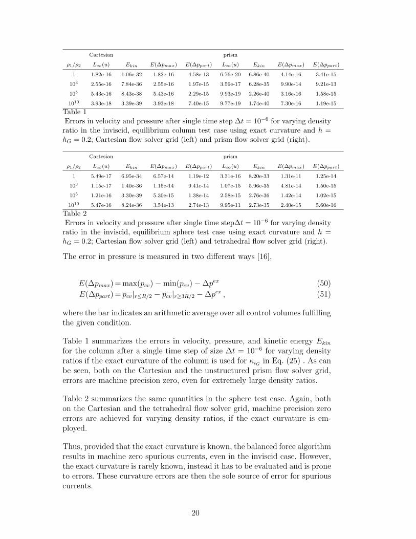
Cartesian prism

ρ1/ρ2 L∞(u) Ekin E(∆pmax) E(∆ppart) L∞(u) Ekin E(∆pmax) E(∆ppart)

1 1.82e-16 1.06e-32 1.82e-16 4.58e-13 6.76e-20 6.86e-40 4.14e-16 3.41e-15

103 2.55e-16 7.84e-36 2.55e-16 1.97e-15 3.59e-17 6.28e-35 9.90e-14 9.21e-13

105 5.43e-16 8.43e-38 5.43e-16 2.29e-15 9.93e-19 2.26e-40 3.16e-16 1.58e-15

1010 3.93e-18 3.39e-39 3.93e-18 7.40e-15 9.77e-19 1.74e-40 7.30e-16 1.19e-15

Table 1Errors in velocity and pressure after single time step ∆t = 10−6 for varying density

ratio in the inviscid, equilibrium column test case using exact curvature and h =hG = 0.2; Cartesian flow solver grid (left) and prism flow solver grid (right).

Cartesian prism

ρ1/ρ2 L∞(u) Ekin E(∆pmax) E(∆ppart) L∞(u) Ekin E(∆pmax) E(∆ppart)

1 5.49e-17 6.95e-34 6.57e-14 1.19e-12 3.31e-16 8.20e-33 1.31e-11 1.25e-14

103 1.15e-17 1.40e-36 1.15e-14 9.41e-14 1.07e-15 5.96e-35 4.81e-14 1.50e-15

105 1.21e-16 3.30e-39 5.30e-15 1.38e-14 2.58e-15 2.76e-36 1.42e-14 1.02e-15

1010 5.47e-16 8.24e-36 3.54e-13 2.74e-13 9.95e-11 2.73e-35 2.40e-15 5.60e-16

Table 2Errors in velocity and pressure after single time step∆t = 10−6 for varying density

ratio in the inviscid, equilibrium sphere test case using exact curvature and h =hG = 0.2; Cartesian flow solver grid (left) and tetrahedral flow solver grid (right).

The error in pressure is measured in two different ways [16],

E(∆pmax) = max(pcv)−min(pcv)−∆pex (50)

E(∆ppart) = pcv|r≤R/2 − pcv|r≥3R/2 −∆pex , (51)

where the bar indicates an arithmetic average over all control volumes fulfillingthe given condition.

Table 1 summarizes the errors in velocity, pressure, and kinetic energy Ekinfor the column after a single time step of size ∆t = 10−6 for varying densityratios if the exact curvature of the column is used for κiG in Eq. (25) . As canbe seen, both on the Cartesian and the unstructured prism flow solver grid,errors are machine precision zero, even for extremely large density ratios.

Table 2 summarizes the same quantities in the sphere test case. Again, bothon the Cartesian and the tetrahedral flow solver grid, machine precision zeroerrors are achieved for varying density ratios, if the exact curvature is em-ployed.

Thus, provided that the exact curvature is known, the balanced force algorithmresults in machine zero spurious currents, even in the inviscid case. However,the exact curvature is rarely known, instead it has to be evaluated and is proneto errors. These curvature errors are then the sole source of error for spuriouscurrents.

20

R

R1

G=0

G=R1-RhG

Fig. 7. Inherent phase interface curvature error when evaluating curvature at nodes.Curvature is determined to be κ = 1/R1 = 1/(R+O(hG)) instead of κ = 1/R.

3.4 RLSG curvature evaluation

As noted in the previous section, only curvature errors result in spurious cur-rents when employing the balanced force algorithm. Hence the task of mini-mizing spurious currents is equivalent to increasing the accuracy of curvatureevaluation. In standard level set methods [44], curvature is evaluated at G-node locations by discretizing Eq. (9),

κ=G2,xx(G

2,y +G2

,z) +G,yy(G2,x +G2

,z) +G,zz(G2,x +G2

,y)

(G2,x +G2

,y +G2,z)

3/2

−2G,xyG,xG,y +G,xzG,xG,z +G,yzG,yG,z

(G2,x +G2

,y +G2,z)

3/2, (52)

typically using a 27-point stencil. It is important to point out that this ap-proach approximates the curvature of the G-isosurface that passes through thenodal point itself. It is therefore, at best, a first-order approximation to thecurvature of the phase interface, which can be a distance hG away from nodesdirectly adjacent to the interface (see Fig. 7). Figures 8 and 9 demonstratethis first-order convergence rate under G-grid refinement for both the columnand the sphere test case using either Cartesian flow solver grids (column andsphere), unstructured prism grids (column), or tetrahedral grids (sphere) withh = 0.2.

Since the root cause of the first-order convergence rate is the fact that curva-ture is not calculated at the interface itself, different approaches can be takento overcome this problem. Introducing a polynomial representation of the in-terface in terms of interface-based coordinates is a viable approach in twodimensions, but becomes cumbersome in three dimensions. Here, we will fol-low an alternative approach using the fact that a quantity defined only on theinterface itself, like curvature, can be distributed to the whole computationaldomain in a meaningful way by solving

∇κ · ∇G = 0 . (53)

21

10-6

10-5

10-4

10-3

10-2

10-1

0.01 0.1hG

cv

10-6

10-5

10-4

10-3

10-2

10-1

0.01 0.1hG

cv

10-6

10-5

10-4

10-3

10-2

10-1

0.01 0.1hG

cv

10-6

10-5

10-4

10-3

10-2

10-1

0.01 0.1hG

cv

Fig. 8. Initial column curvature errors under G-grid refinement; flow solver gridh = 0.2; Cartesian flow solver grid (top), prism flow solver grid (bottom); nodalcurvature (circles), direct front curvature (squares), Chopp front curvature (trian-gles), first- and second-order convergence (dashed lines).

This effectively sets κ constant in the front normal direction. Note that due toEq. (25), Eq. (53) needs to be solved only for G-nodes adjacent to the interface.The problem is therefore similar to determining the initially accepted valuesin the Fast Marching Method [2]. For this purpose, Chopp [10] developed aNewton’s method that determines the nearest point on the interface (called“base-point” in the following) for a given node in two dimensions. The methodrelies on approximating the level set scalar within each computational cellclose to the interface by a bi-cubic spline. For this purpose, G need not bea distance function. We have extended Chopp’s method to three dimensionsusing C1, isotropic tri-cubic interpolations [26]. We typically find the base-point within 2–4 Newton iterations. However, in some situations, the base-point is not in the interior of the region in which the tricubic approximationwas taken but in an adjacent region, also bounded by the same node. In thiscase, the base-point is rejected, unless none of the alternative seven regionsthe node belongs to yields a valid base-point. Once the base-point coordinateshave been determined, the base-point’s curvature is calculated by tri-linearinterpolation using the surrounding nodal curvature values. Using Eq. (53),the nodal curvature is then set equal to its base-point’s curvature.

22

10-6

10-5

10-4

10-3

10-2

10-1

0.01 0.1hG

cv

10-6

10-5

10-4

10-3

10-2

10-1

0.01 0.1hG

cv

10-6

10-5

10-4

10-3

10-2

10-1

0.01 0.1hG

cv

10-6

10-5

10-4

10-3

10-2

10-1

0.01 0.1hG

cv

Fig. 9. Initial sphere curvature errors under G-grid refinement; flow solver gridh = 0.2; Cartesian flow solver grid (top), prism flow solver grid (bottom); nodalcurvature (circles), direct front curvature (squares), Chopp front curvature (trian-gles), first- and second-order convergence (dashed lines).

The resulting curvature errors under G-grid refinement using Chopp’s methodare shown in Figs. 8 and 9. They show second-order convergence, and evenon coarse grids, Chopp’s method yields more than one order of magnitudebetter curvature estimates than the nodal-based evaluation. The drawback ofChopp’s method is that for complex interface geometries in three dimensions,the Newton algorithm does not always converge. The method thus lacks thestability required for complex interface geometries typically found in liquid/gasflows. Thus, the following method is proposed as an alternative.

Assuming that G is smooth in the vicinity of the phase interface, the base-point xB for a given node xG close to the interface can be explicitly calculatedfrom

xB = xG − dn = xG −G

|∇G|∇G|∇G|

, (54)

where all gradients are calculated using central differences. This approach istermed direct front curvature in the following. It gives good base-point esti-mates only for nodes close to the interface. However, due to the way Eq. (25)

23

10-10

10-8

10-6

10-4

10-2

0.01 0.1hG0.01 0.1hG

0.01 0.1hG0.01 0.1hG

column column sphere sphere

Fig. 10. Equilibrium inviscid column and sphere velocity (circle) and pressure (tri-angle) errors after 1 time step ∆t = 10−6 under G-grid refinement; flow solver gridh = 0.2, density ratio ρ1/ρ2 = 103; from left and right: column Cartesian flow solvergrid, column prism flow solver grid, sphere Cartesian flow solver grid, and spheretetrahedral flow solver grid; dashed lines mark second-order convergence.

is evaluated, κ needs to be calculated only on nodes close to the interface,making the direct front curvature method viable. As before, once base-pointshave been determined, their curvature is again calculated using tri-linear in-terpolation from the surrounding nodal curvature values. Then, according toEq. (53), the curvature values of nodes are set to their respective base-points’curvature values. Figures 8 and 9 also include the curvature errors calculatedby the direct method. As can be seen, they are virtually indistinguishable fromthe values obtained using Chopp’s method yielding second-order convergence.

Comparing the obtained curvature errors to those calculated by Francois etal. [16], both Chopp’s and the direct method give curvature errors an approx-imate factor of 5 lower than the 7x3 stencil height function method employedin that paper. While a height function approach could be employed in theRLSG method as well, since volume fractions ψ are readily available, the ef-fective G-stencil needed would be 9x5x5 (cf. Eqs. 17 - 19), as compared to4x4x4 in the direct front curvature method. Smaller stencil sizes are especiallyimportant for complex interface geometries, since both the height function andall level set curvature methods are based on the assumption that all ψ and Gvalues in the stencil relate to one continuous interface segment only. Auxiliary,non-contiguous, interface segments inside the stencil can introduce significanterrors. These can only be avoided by temporarily removing the auxiliary inter-face segments during curvature calculation. Such methods have been recentlyproposed by Macklin and Lowengrub [28] for level sets and Sussman and Ohta[50] for height functions.

In the following, we will employ the direct front curvature method to calculatenodal curvature values on the G-grid. Figure 10 shows the errors in velocityand pressure after a single time step of size ∆t = 10−6, using ρ1 = 1 andρ2 = 10−3 and refining the resolution hG of the G-grid. As expected, due tothe balanced force algorithm, errors in curvature evaluation result in errorsin velocity and pressure, showing the same second-order convergence behavior

24

(cf. Figs. 8 and 9).

3.5 RLSG parallel implementation and load balancing

Parallel efficiency and scalability is key to allow extremely high resolution G-grids. In typical applications involving tracked interfaces, interfaces make upa small fraction of the flow solver volume only. Furthermore, the region occu-pied by the interface is not static. An efficient domain decomposition strategyfor the flow solver is thus usually inefficient for the RLSG solver and viceversa. Dual constraint partitioning is possible, however, the dynamic move-ment of the interface through the flow solver domain would require frequentjoined repartitioning of the G-grid and the otherwise static flow solver grid.Therefore, we propose to use independent partitioning for the flow solver gridand the G-grid. The former is domain decomposed at the beginning of a sim-ulation and retains its partitioning throughout the simulation. The latter isdynamically decomposed and load balanced throughout the simulation, oncea load-imbalance factor is greater than some threshold value.

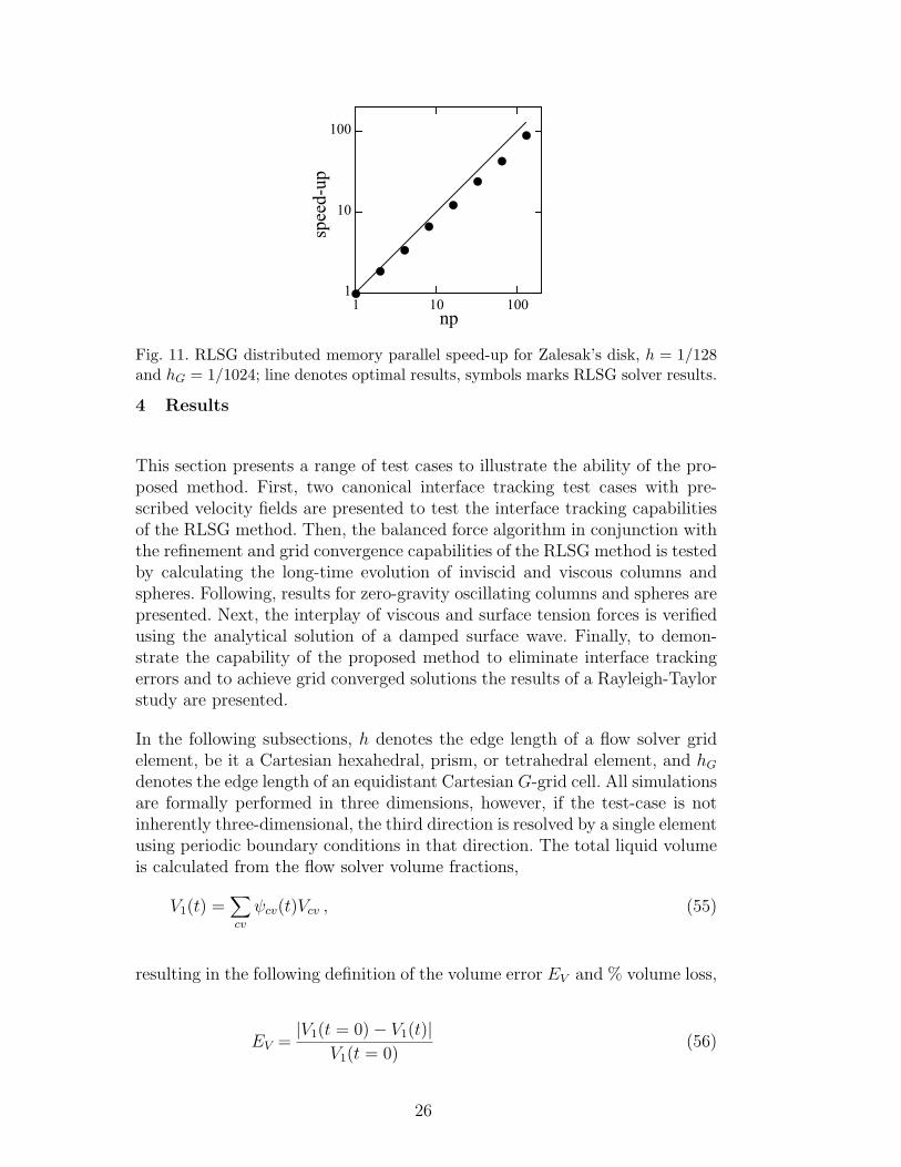
Domain decomposition of the G-grid is straightforward using the super-grid.At the beginning of the simulation, all super-grid cells, active or not, areassigned to a processor and the negative value of the processor rank is storedin a super-grid i,j,k lookup table that is synchronized on all processors. Thus,if a band grows into a previously not activated super-grid block, a uniqueprocessor is already assigned to this block. After the band regeneration step,this strategy can lead to a load-imbalance in terms of number of local activecells inside the T - and N -band. To re-loadbalance, the processor with thelargest number of active cells sends its super-grid block containing the mostactive cells to the processor with the smallest number of active cells. Thisprocess is repeated until either the threshold imbalance factor is reached, orthe load balance does not decrease any more. Then, the super-grid i,j,k lookuptable is synchronized to reflect any changed super-grid block processor ranks.Note that more advanced strategies also minimizing the domain edge countcan be devised, however the strategy outlined above leads to good parallelperformance and load-balance. Figure 11 shows the parallel scalability of theRLSG solver using Zalesak’s disk test case described in a later section with aCartesian flow solver grid of h = 1/128 and a G-grid of hG = 1/1024. A nearlyconstant, although slightly sub-optimal speed-up is observed over all countsof processors np.

25

1

10

100

1 10 100np

speed-up

Fig. 11. RLSG distributed memory parallel speed-up for Zalesak’s disk, h = 1/128and hG = 1/1024; line denotes optimal results, symbols marks RLSG solver results.

4 Results

This section presents a range of test cases to illustrate the ability of the pro-posed method. First, two canonical interface tracking test cases with pre-scribed velocity fields are presented to test the interface tracking capabilitiesof the RLSG method. Then, the balanced force algorithm in conjunction withthe refinement and grid convergence capabilities of the RLSG method is testedby calculating the long-time evolution of inviscid and viscous columns andspheres. Following, results for zero-gravity oscillating columns and spheres arepresented. Next, the interplay of viscous and surface tension forces is verifiedusing the analytical solution of a damped surface wave. Finally, to demon-strate the capability of the proposed method to eliminate interface trackingerrors and to achieve grid converged solutions the results of a Rayleigh-Taylorstudy are presented.

In the following subsections, h denotes the edge length of a flow solver gridelement, be it a Cartesian hexahedral, prism, or tetrahedral element, and hGdenotes the edge length of an equidistant Cartesian G-grid cell. All simulationsare formally performed in three dimensions, however, if the test-case is notinherently three-dimensional, the third direction is resolved by a single elementusing periodic boundary conditions in that direction. The total liquid volumeis calculated from the flow solver volume fractions,

V1(t) =∑cv

ψcv(t)Vcv , (55)

resulting in the following definition of the volume error EV and % volume loss,

EV =|V1(t = 0)− V1(t)|

V1(t = 0)(56)

26

90

80

70

60

30 40 50 60 70 30 40 50 60 70 30 40 50 60 70 30 40 50 60 70

Fig. 12. Zalesak’s disk after one full rotation with h = 1; exact solution (thin line)and hG = 1, hG = 1/2, hG = 1/4, and hG = 1/8 (from left to right).

% volume loss =V1(t = 0)− V1(t)

V1(t = 0)· 100% . (57)

The shape error Eshape is a measure for the amount of fluid that has prop-agated to the wrong side of the exact interface location. It is calculated byfirst dividing each G-grid cell into 1000 sub-cells in each coordinate direction,using tri-linear interpolation to calculate the level set scalar value Gs at eachsub-cell centroid, and then evaluating

Eshape(t) =1L

∑iG

∑sub−cells |H(Gs(t))−H(Gs(t = 0))|Vsub−cell

2∑iG ViG

, (58)

with L the exact interface length or area at t = 0.

4.1 Zalesak’s disk

The solid body rotation of a notched circle, also known as Zalesak’s disk [61],is one of the standard test problems for evaluating the accuracy of level setmethods in maintaining sharp corners. A disk of radius 15, notch width 5, andnotch height 25 is placed in a 100 × 100 box at (50, 75). The velocity field isgiven by

u(x, t) = (50− y, x− 50)T (59)

and the flow solver constant time step size is set to ∆t = 2π/628. Figure 12shows the shape of the interface at t = 2π after one full rotation of the diskusing an equidistant Cartesian flow solver grid with h = 1. Due to the linearityof the imposed velocity field, results for the flow solver prism grid are identicalto those of the Cartesian flow solver grid and are thus not shown here. As istypical of level set methods, the sharp corners of the notched disk tend tobe rounded, however, the overall shape of the notch is well preserved, evenon the coarsest G-grid of hG = 1. Refining the G-grid continuously improvesthe shape, until for the finest G-grid resolution visually no difference can be

27

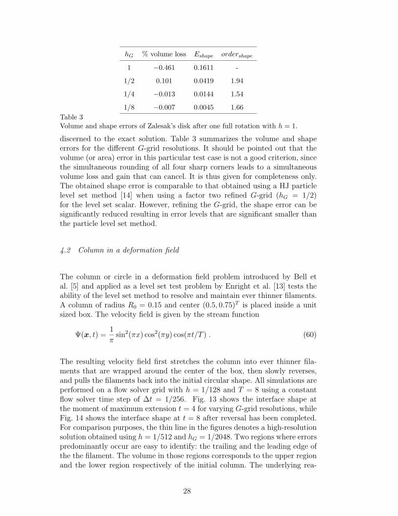
hG % volume loss Eshape ordershape

1 −0.461 0.1611 -

1/2 0.101 0.0419 1.94

1/4 −0.013 0.0144 1.54

1/8 −0.007 0.0045 1.66Table 3Volume and shape errors of Zalesak’s disk after one full rotation with h = 1.

discerned to the exact solution. Table 3 summarizes the volume and shapeerrors for the different G-grid resolutions. It should be pointed out that thevolume (or area) error in this particular test case is not a good criterion, sincethe simultaneous rounding of all four sharp corners leads to a simultaneousvolume loss and gain that can cancel. It is thus given for completeness only.The obtained shape error is comparable to that obtained using a HJ particlelevel set method [14] when using a factor two refined G-grid (hG = 1/2)for the level set scalar. However, refining the G-grid, the shape error can besignificantly reduced resulting in error levels that are significant smaller thanthe particle level set method.

4.2 Column in a deformation field

The column or circle in a deformation field problem introduced by Bell etal. [5] and applied as a level set test problem by Enright et al. [13] tests theability of the level set method to resolve and maintain ever thinner filaments.A column of radius R0 = 0.15 and center (0.5, 0.75)T is placed inside a unitsized box. The velocity field is given by the stream function

Ψ(x, t) =1

πsin2(πx) cos2(πy) cos(πt/T ) . (60)

The resulting velocity field first stretches the column into ever thinner fila-ments that are wrapped around the center of the box, then slowly reverses,and pulls the filaments back into the initial circular shape. All simulations areperformed on a flow solver grid with h = 1/128 and T = 8 using a constantflow solver time step of ∆t = 1/256. Fig. 13 shows the interface shape atthe moment of maximum extension t = 4 for varying G-grid resolutions, whileFig. 14 shows the interface shape at t = 8 after reversal has been completed.For comparison purposes, the thin line in the figures denotes a high-resolutionsolution obtained using h = 1/512 and hG = 1/2048. Two regions where errorspredominantly occur are easy to identify: the trailing and the leading edge ofthe the filament. The volume in those regions corresponds to the upper regionand the lower region respectively of the initial column. The underlying rea-

28

0.9

0.7

0.5

0.3

0.10.1 0.3 0.5 0.7 0.9 0.1 0.3 0.5 0.7 0.9 0.1 0.3 0.5 0.7 0.9 0.1 0.3 0.5 0.7 0.9

Fig. 13. Interface shape of column in a deformation field at t = T/2, h = 1/128; tar-get solution (thin line) and hG = 1/128, hG = 1/256, hG = 1/512, and hG = 1/1024(from left to right).

0.9

0.8

0.7

0.6

0.3 0.4 0.5 0.6 0.7 0.3 0.4 0.5 0.6 0.7 0.3 0.4 0.5 0.6 0.7 0.3 0.4 0.5 0.6 0.7

Fig. 14. Interface shape of column in a deformation field at t = T , h = 1/128; targetsolution (thin line) and hG = 1/128, hG = 1/256, hG = 1/512, and hG = 1/1024(from left to right).

son for the poor volume conservation in the coarse G-grid case (hG = 1/128)is two-fold. For one, the incorrect merging of characteristics in the transportstep, but especially during re-initialization moves the interface, resulting inannihilation of thin filament structures. But even if perfect transport andre-initialization could be performed, the hG = 1/128 solution would loose sig-nificant amounts of volume because the trailing filament thickness falls belowthe grid resolution of hG = 1/128 and is thus not resolvable by a fixed gridmethod.

Continuously refining the G-grid results in ever better shape and volumepreservation, resulting in roughly second-order grid convergence under G-gridrefinement, see Tab. 4. The obtained results compare well to the HJ particlelevel set method [14], resulting in slightly larger errors for a factor 2 finerG-grid and slightly smaller errors for a factor 4 refined G-grid.

Table 5 summarizes the results obtained using a prism flow solver grid. Sincethe prescribed velocity field is not linear, the employed tri-linear interpolationon a Cartesian and a prism element causes minute differences. While the in-terface shapes presented in Figs. 13 and 14 look visually identical, the errornorms show a slight increase in error for the prism case.

29

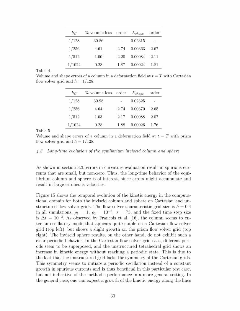
hG % volume loss order Eshape order

1/128 30.86 - 0.02315 -

1/256 4.61 2.74 0.00363 2.67

1/512 1.00 2.20 0.00084 2.11

1/1024 0.28 1.87 0.00024 1.81Table 4Volume and shape errors of a column in a deformation field at t = T with Cartesianflow solver grid and h = 1/128.

hG % volume loss order Eshape order

1/128 30.98 - 0.02325 -

1/256 4.64 2.74 0.00370 2.65

1/512 1.03 2.17 0.00088 2.07

1/1024 0.28 1.88 0.00026 1.76Table 5Volume and shape errors of a column in a deformation field at t = T with prismflow solver grid and h = 1/128.

4.3 Long-time evolution of the equilibrium inviscid column and sphere

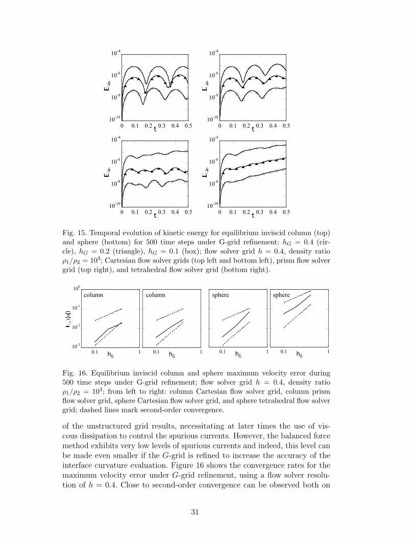
As shown in section 3.3, errors in curvature evaluation result in spurious cur-rents that are small, but non-zero. Thus, the long-time behavior of the equi-librium column and sphere is of interest, since errors might accumulate andresult in large erroneous velocities.

Figure 15 shows the temporal evolution of the kinetic energy in the computa-tional domain for both the inviscid column and sphere on Cartesian and un-structured flow solver grids. The flow solver characteristic grid size is h = 0.4in all simulations, ρ1 = 1, ρ2 = 10−3, σ = 73, and the fixed time step sizeis ∆t = 10−3. As observed by Francois et al. [16], the column seems to en-ter an oscillatory mode that appears quite stable on a Cartesian flow solvergrid (top left), but shows a slight growth on the prism flow solver grid (topright). The inviscid sphere results, on the other hand, do not exhibit such aclear periodic behavior. In the Cartesian flow solver grid case, different peri-ods seem to be superposed, and the unstructured tetrahedral grid shows anincrease in kinetic energy without reaching a periodic state. This is due tothe fact that the unstructured grid lacks the symmetry of the Cartesian grids.This symmetry seems to initiate a periodic oscillation instead of a constantgrowth in spurious currents and is thus beneficial in this particular test case,but not indicative of the method’s performance in a more general setting. Inthe general case, one can expect a growth of the kinetic energy along the lines

30

10-10

10-8

10-6

10-4

0 0.1 0.2 0.3 0.4 0.5t10-10

10-8

10-6

10-4

0 0.1 0.2 0.3 0.4 0.5t

10-10

10-8

10-6

10-4

0 0.1 0.2 0.3 0.4 0.5t10-10

10-8

10-6

10-4

0 0.1 0.2 0.3 0.4 0.5t

Fig. 15. Temporal evolution of kinetic energy for equilibrium inviscid column (top)and sphere (bottom) for 500 time steps under G-grid refinement: hG = 0.4 (cir-cle), hG = 0.2 (triangle), hG = 0.1 (box); flow solver grid h = 0.4, density ratioρ1/ρ2 = 103; Cartesian flow solver grids (top left and bottom left), prism flow solvergrid (top right), and tetrahedral flow solver grid (bottom right).

column column sphere sphere

10-3

10-2

10-1

100

0.1 1hG0.1 1hG

0.1 1hG0.1 1hG

Fig. 16. Equilibrium inviscid column and sphere maximum velocity error during500 time steps under G-grid refinement; flow solver grid h = 0.4, density ratioρ1/ρ2 = 103; from left to right: column Cartesian flow solver grid, column prismflow solver grid, sphere Cartesian flow solver grid, and sphere tetrahedral flow solvergrid; dashed lines mark second-order convergence.

of the unstructured grid results, necessitating at later times the use of vis-cous dissipation to control the spurious currents. However, the balanced forcemethod exhibits very low levels of spurious currents and indeed, this level canbe made even smaller if the G-grid is refined to increase the accuracy of theinterface curvature evaluation. Figure 16 shows the convergence rates for themaximum velocity error under G-grid refinement, using a flow solver resolu-tion of h = 0.4. Close to second-order convergence can be observed both on

31

La 12 120 1200 12000 120000 1200000

Ca Cartesian 0.10e-6 0.11e-6 0.12e-6 1.44e-6 3.09e-6 0.71e-6

Ca [39] 6.76e-6 5.71e-6 5.99e-6 8.76e-6 - -

Ca [45] 2.18e-6 2.18e-6 2.18e-6 2.22e-6 - -

Ca prism 0.15e-6 0.15e-6 0.16e-6 2.17e-6 3.93e-6 0.96e-6

Ca [30] 85.1e-6 86.2e-6 85.9e-6 83.1e-6 - -Table 6Dependence of the spurious current capillary number on the Laplace number forviscous equilibrium column and D/h = D/hG = 12.8 as compared to Popinet andZaleski [39] and Shin et al. [45] on Cartesian grid (top) and Marchandise et al.(D/h = 16) [30] on prism grid.

structured and unstructured flow solver grids.

4.4 Long time evolution of the viscous equilibrium column and sphere

To evaluate the performance of the proposed RLSG balanced force methodas compared to other numerical methods, we perform simulations of the longtime evolution of viscous columns and spheres at equilibrium. A column ofdiameter D = 0.4 is placed in the center of a unit sized box resolved byeither Cartesian or prism cells with h = 1/32. The viscosity in both fluidsis set to µ = 0.1 and the surface tension coefficient is set to σ = 1. TheLaplace number La = 1/Oh2 = σρD/µ2 is varied by changing the density inboth fluids, keeping the density ratio fixed as ρ1/ρ2 = 1. The time step sizeis chosen to be ∆t = ∆tcap/2, see Eq. (42). Table 6 compares the capillarynumber Ca = |umax|µ/σ for varying Laplace numbers at tσ/(Dµ) = 250using a Cartesian flow solver grid to the benchmark results of Popinet andZaleski [39] using a marker tracking method and Shin et al. [45] using a levelcontouring approach. The table also shows results obtained on the prism gridcompared to the results of Marchandise et al. [30] employing a finite elementmethod on a slightly finer unstructured grid. Results with the RLSG methodshow more than one order of magnitude smaller spurious currents for smallervalues of the Laplace numbers on Cartesian grids, and more than two-ordersof magnitude better results on non-Cartesian grids. However, at very largeLaplace numbers, the present results are not fully independent of the Laplacenumber due to small, decaying periodic oscillations in the spurious currentmagnitude that are present in the inviscid case as well, see Fig. 15.

Table 7 analyzes the grid convergence behavior. Again, the spurious currentsof the RLSG method are significantly lower than those reported by Popinetand Zaleski [39] and convergence under grid refinement is roughly second or-

32

h, hG 1/16 1/32 1/64 1/128

Ca 4.92e-6 1.44e-6 0.34e-6 0.05e-6

Ca [39] 37.60e-5 6.68e-6 1.07e-6 0.12e-6Table 7Grid convergence of the spurious current capillary number for viscous equilibriumcolumn and 1/Oh2 = 12000 compared to the results by Popinet and Zaleski [39].

∆t/∆tcap 1 1/2 1/4 1/8

Ca 0.12e-6 0.12e-6 0.12e-6 0.13e-6Table 8Time step convergence of the spurious current capillary number for viscous equilib-rium column at h = hG = 1/32 and 1/Oh2 = 1200.

hG 1/16 1/32 1/64 1/128

Ca 4.92e-6 4.46e-6 2.10e-6 8.92e-7

order - 0.14 1.09 1.24Table 9Grid convergence of the spurious current capillary number for viscous equilibriumcolumn, 1/Oh2 = 12000, and fixed flow solver grid h = 1/16.

der. Table 8 demonstrates that the reported capillary numbers are virtuallyindependent of the chosen time step size, even for timestep sizes close to thestability limit.

Finally, Table 9 shows the spurious current capillary number for a fixed flowsolver grid under G-grid refinement using a time step of ∆t = 0.9∆tcap with∆tcap based on the flow solver grid size h = 1/16. The results demonstratethat the capillary time step restriction is not based on the RLSG grid size hG,but rather on the flow solver grid size h as expected, since at the finest G-grid (hG = 1/128), the employed time step is more than 20 times larger thana stable capillary time step based on hG. Overall convergence under G-gridrefinement is approximately first order.

As a three dimensional test, the viscous sphere of Renardy and Renardy [42]is calculated. Here, a sphere of diameter D = 0.25 is placed at the center ofa unit sized Cartesian box with symmetry boundary conditions at all sides.The surface tension coefficient is set to σ = 0.357, density and viscosity inboth fluids are ρ = 4 and µ = 1, resulting in a Laplace number of 1/Oh2 =0.357. The time step size is ∆t = 10−5 and the simulation is run for 200 timesteps. Table 10 compares the maximum spurious current capillary number att = 0.002 to those obtained by Renardy and Renardy [42] using the PROSTVolume of Fluid algorithm on a staggered mesh. Although the RLSG methodresults in slightly smaller values, both methods yield comparable, high qualityresults.

33

h, hG 1/96 1/128 1/160 1/192

Ca 4.82e-5 3.44e-5 2.02e-5 1.43e-5

Ca [42] 6.28e-5 3.67e-5 2.67e-5 1.59e-5Table 10Grid convergence of the spurious current capillary number for viscous equilibriumsphere with parameters due to Renardy and Rendary [42].

4.5 Zero gravity column/drop oscillation

To further verify the implementation of the balanced force algorithm, thissection presents results for zero gravity oscillating columns and spheres. Thetheoretical oscillation period for columns in the linear regime is given by [25]

ω2 =n(n2 − 1)σ

(ρ1 + ρ2)R30

, (61)

while that for spheres can be calculated from [25]

ω2 =n(n2 − 1)(n+ 2)σ

[(n+ 1)ρ1 + nρ2]R30

. (62)

In all simulations a column respectively sphere of radius R0 = 2 is placed inthe center of a [−10, 10] square box with slip boundary conditions on all sidesand σ = 1, ρ1 = 1, ρ2 = 0.01, µ1 = 0.01, and µ2 = 1 · 10−4, resulting in aLaplace number of La = 20000. The column/sphere is initially perturbed by amode n = 2 pertubation with an initial amplitude of A0 = 0.01R0. The timestep size in all simulations is chosen as ∆t = 0.5∆tcap.

Table 11 shows the period of oscillation error ET = |Tcalcω/2π − 1| for theoscillating column together with the results reported by Torres and Brackbill[55], whereas Table 13 lists the corresponding results for the oscillating sphere.Results better by a factor of roughly 2 are obtained even on prism grids ascompared to the results reported in [55] and the oscillating sphere results showsecond order grid convergence. Table 12 analyzes the temporal convergence.Simulations are stable even at the capillary time step limit and show slightlybetter than first order convergence under time step refinement.

4.6 Damped surface waves

To verify the interplay of the surface tension term with the viscous termswe compare the results of the proposed method to the initial value theory

34

h, hG 20/64 20/128 20/256

ET Cartesian 4.04e-2 1.05e-2 0.37e-2

ET prism 5.91e-2 1.65e-2 1.36e-2

ET [55] 13.2e-2 6.1e-2 1.5e-2Table 11Zero gravity 2D column oscillation. Error in oscillation period as compared to lineartheory [25].

∆t/∆tcap 1 1/2 1/4 1/8

ET 4.26e-2 4.04e-2 3.90e-2 3.85e-2Table 12Zero gravity 2D column oscillation. Error in oscillation period on Cartesian gridh = hG = 20/64 as compared to linear theory [25].

h, hG 20/64 20/96 20/128 20/160

ET 8.50e-2 3.85e-2 2.08e-2 1.19e-2

order - 1.95 2.14 2.50Table 13Zero gravity 3D sphere oscillation. Error in oscillation period on Cartesian grid ascompared to linear theory [25].

of Prosperetti [40] for a small amplitude damped surface wave between twosuperposed immiscible fluids. The initial surface position inside a [0, 2π] ×[0, 2π] box is given by a sinusoidal disturbance of wavelength λ = 2π andamplitude A0 = 0.01λ,

G(x, t = 0) = y − y0 + A0 cos(x− hG/2) , (63)

with y0 = π. Periodic boundary conditions are used in the x-direction and slipwalls are imposed in the y-direction. The initial value solution for two fluidswith equal kinematic viscosity ν and λ = 2π can be written as [40]

Aex(t) =4(1− 4β)ν2

8(1− 4β)ν2 + ω20

A0erfc√νt+

4∑i=1

ziZi

(ω2

0A0

z2i − ν

)exp[(z2

i − ν)t]erfc(zi√t) , (64)

where zi are the roots of

z4 − 4β√νz3 + 2(1− 6β)νz2+

4(1− 3β)ν3/2z + (1− 4β)ν2 + ω20 = 0 , (65)

35

-0.01

-0.005

0

0.005

0.01

0 4 8 12 16 20 24

A/!

t

-0.01

-0.005

0

0.005

0.01

0 4 8 12 16 20 24

A/!

t

Fig. 17. Amplitude A of damped surface wave with ρ1/ρ2 = 1; Cartesian grid (left)and prism grid (right) with h = hG = λ/16 (dashed), h = hG = λ/32 (dash-dot),h = hG = λ/64 (dotted), h = hG = λ/128 (solid), and theory (thin line).

-0.4

-0.2

0

0.2

0.4

0 4 8 12 16 20 24

E

t

-0.4

-0.2

0

0.2

0.4

0 4 8 12 16 20 24

E

t

Fig. 18. Amplitude error E of damped surface wave with ρ1/ρ2 = 1; Cartesiangrid (left) and prism grid (right) with h = hG = λ/16 (dashed), h = hG = λ/32(dash-dot), h = hG = λ/64 (dotted), h = hG = λ/128 (solid), and theory (thinline).

the dimensionless parameter β is given by β = ρ1ρ2/(ρ1 + ρ2)2, the inviscidoscillation frequency is ω0 =

√σ

ρ1+ρ2, and Zi =

∏4j=1j 6=i

(zj − zi).

We analyze two different cases for σ = 2, the first where both fluids have equaldensity, ρ1 = ρ2 = 1 and ν = 0.064720863, and the second where the two fluidshave a high density ratio, ρ1 = 1000, ρ2 = 1, and ν = 0.0064720863. Resultsare obtained using a fixed time step size of ∆t = 0.003 in the equal densitycase and ∆t = 0.06 in the high density ratio case. In both cases we perform atleast one re-initialization step, i.e. we force the initial re-initialization triggercondition to be true, cp. Fig. 2.

Figure 17 shows the temporal evolution of the non-dimensional disturbanceamplitude A measured at x = hG/2 under flow solver and G-grid refinementfor both a Cartesian and a prism flow solver grid for the case of equal densities,whereas Fig. 18 shows the evolution of the corresponding non-dimensional er-ror E(t) = (A(t)−Aex(t))/A0, and Tab. 14 summarizes its root mean square.

36

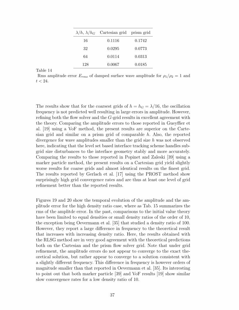
λ/h, λ/hG Cartesian grid prism grid

16 0.1116 0.1742

32 0.0295 0.0773

64 0.0114 0.0313

128 0.0067 0.0185Table 14Rms amplitude error Erms of damped surface wave amplitude for ρ1/ρ2 = 1 andt < 24.

The results show that for the coarsest grids of h = hG = λ/16, the oscillationfrequency is not predicted well resulting in large errors in amplitude. However,refining both the flow solver and the G-grid results in excellent agreement withthe theory. Comparing the amplitude errors to those reported in Gueyffier etal. [19] using a VoF method, the present results are superior on the Carte-sian grid and similar on a prism grid of comparable h. Also, the reporteddivergence for wave amplitudes smaller than the grid size h was not observedhere, indicating that the level set based interface tracking scheme handles sub-grid size disturbances to the interface geometry stably and more accurately.Comparing the results to those reported in Popinet and Zaleski [39] using amarker particle method, the present results on a Cartesian grid yield slightlyworse results for coarse grids and almost identical results on the finest grid.The results reported by Gerlach et al. [17] using the PROST method showsurprisingly high grid convergence rates and are thus at least one level of gridrefinement better than the reported results.

Figures 19 and 20 show the temporal evolution of the amplitude and the am-plitude error for the high density ratio case, where as Tab. 15 summarizes therms of the amplitde error. In the past, comparisons to the initial value theoryhave been limited to equal densities or small density ratios of the order of 10,the exception being Oevermann et al. [35] that studied a density ratio of 100.However, they report a large difference in frequency to the theoretical resultthat increases with increasing density ratio. Here, the results obtained withthe RLSG method are in very good agreement with the theoretical predictionsboth on the Cartesian and the prism flow solver grid. Note that under gridrefinement, the amplitude errors do not appear to converge to the exact the-oretical solution, but rather appear to converge to a solution consistent witha slightly different frequency. This difference in frequency is however orders ofmagnitude smaller than that reported in Oevermann et al. [35]. Its interestingto point out that both marker particle [39] and VoF results [19] show similarslow convergence rates for a low density ratio of 10.

37

-0.01

-0.005

0

0.005

0.01

0 100 200 300 400

A/!

t

-0.01

-0.005

0

0.005

0.01

0 100 200 300 400

A/!

t

Fig. 19. Amplitude A of damped surface wave with ρ1/ρ2 = 1000; Cartesian grid(left) and prism grid (right) with h = hG = λ/16 (dashed), h = hG = λ/32(dash-dot), h = hG = λ/64 (dotted), h = hG = λ/128 (solid), and theory (thinline).

-0.15

-0.10

-0.05

0

0.05

0.10

0.15

0 100 200 300 400

E

t

-0.15

-0.10

-0.05

0

0.05

0.10

0.15

0 100 200 300 400

E

t

Fig. 20. Amplitude error E of damped surface wave with ρ1/ρ2 = 1000; Cartesiangrid (left) and prism grid (right) with h = hG = λ/16 (dashed), h = hG = λ/32(dash-dot), h = hG = λ/64 (dotted), h = hG = λ/128 (solid), and theory (thinline).

λ/h, λ/hG Cartesian grid prism grid

16 0.0482 0.0564

32 0.0208 0.0141

64 0.0127 0.0113

128 0.0118 0.0157Table 15Relative rms error Erms/A0 of damped surface wave amplitude for ρ1/ρ2 = 1000

and t < 450.

4.7 Rayleigh-Taylor instability

To demonstrate the performance of the proposed method in a more complexflow, a Rayleigh-Taylor instability is computed. This is a common test problem

38

0 1-2

-1

0

1

2t = 0.5 t = 0.6 t = 0.7 t = 0.8 t = 0.9

Fig. 21. Rayleigh-Taylor instability interface shapes for reference solution,h = hG = 1/512 .

performed by a variety of different methods [6,18,39,41]. A heavy fluid, ρ1 =1.225, µ1 = 0.00313, is placed above a light fluid, ρ2 = 0.1694, µ2 = 0.00313,inside a domain of size 1x4. The interface between the two fluids is placed inthe middle of the domain and is perturbed by a cosine wave of amplitude 0.05.The gravity constant is set to g = 9.81. We set the time step size constant to∆t = 2.5 ·10−4 and simulate up to t = 0.9. Figure 21 shows the interface shapeat different instances in time for a Cartesian flow solver grid of h = 1/512 anda G-grid of hG = 1/512. As will be demonstrated below, this grid resolutionensures grid converged results and thus will be used as a reference solution inthe following.

Figures 22–24 show the interface shape for different resolutions of the flowsolver grid and G-grid, whereas Figs. 25–27 show the corresponding resultsfor prism flow solver grids. Using the coarsest Cartesian flow solver grid ofh = 1/64 presented in Fig. 22, one can already notice deviations from thereference solution at early times. While the stem and bubble shape is wellcaptured, the fine scale geometry of the side arms is not well maintained.Up to t = 0.8, there appears almost no difference between the results usinghG ≥ 1/128. This indicates that the deviations from the reference solution aredue to errors in the flow representation and not due to errors in the interfacetracking scheme. However, at t = 0.9, the very fine connecting bridge at theside arms can only be maintained by hG = 1/512. Note that except for thedifference in the details of the connecting bridge, the larger scale geometricfeatures are consistent between different G-grid resolution with hG ≥ 1/128.

39

-1.0

-0.5

0

0.5-1.5

-1.0

-0.5

1

hG=1/64

t=0.6 t=0.7

t=0.8 t=0.9

1/128

1/128

1/128

1/128

1/256

1/256

1/512

1/512

1/256

1/256

1/512

1/512hG=1/64

hG=1/64

hG=1/64

Fig. 22. Rayleigh-Taylor instability interface shapes under G-grid refinement hG =1/64, 1/128, 1/256, and 1/512 (left to right in each group) at t = 0.6, 0.7, 0.8, and0.9 (top left to bottom right) and Cartesian flow solver grid h = 1/64. Thin linedenotes reference solution.

Figure 25 shows the corresponding results for a prism flow solver grid of h =1/64. The obtained interface shapes are noticeable worse than in the Cartesiancase showing deviations even in the lower stem and bubble shape. Again, goodinterface grid convergence is achieved for hG ≥ 1/128 up to t = 0.8, indicatingthat the observed deviations from the reference solution are due to insufficientflow solver resolution. Note that at t = 0.9, the hG = 1/512 grid is not ableto maintain the thin connecting bridge, since it is thinner than the referencesolution.

At a Cartesian flow solver grid of h = 1/128 presented in Fig. 23, virtually nodifference can be discerned between the reference solution and G-grid resolu-tions of hG ≥ 1/128 up to t = 0.8. At t = 0.9, however, the thin connectingbridge is only supported by hG = 1/512. Comparing the results at t = 0.9 ofh = 1/128 to those of h = 1/64 (cf. Fig. 22), the finer grid flow solver resultscapture the shape of the interface significantly better. This indicates that theflowfield is well resolved by the h = 1/128 grid. This conclusion is even moreevident in the prism flow solver case when comparing the h = 1/128 solu-tion, Fig. 26, to the h = 1/64 solution, Fig. 25. At h = 1/128 both the stemshape and the bubble shape are well captured. Yet, although the interfaceshapes converge well for hG ≥ 1/256, there still exists a noticeable differenceto the reference solution at the outside edges of the bubble, indicating thatthe employed prism grid might be insufficient to resolve the fine scale flowfield there.

Refining the Cartesian flow solver grid further to h = 1/256, presented in Fig.

40

-1.0

-0.5

0

0.5-1.5

-1.0

-0.5

1

hG=1/128

t=0.6 t=0.7

t=0.8 t=0.9

hG=1/128

hG=1/128

hG=1/128

1/256 1/512 1/256 1/512

1/256 1/512 1/256 1/512

Fig. 23. Rayleigh-Taylor instability interface shapes under G-grid refinement hG =1/128, 1/256, and 1/512 (left to right in each group) at t = 0.6, 0.7, 0.8, and 0.9 (topleft to bottom right) and Cartesian flow solver grid h = 1/128. Thin line denotesreference solution.

-1.0

-0.5

0

hG=1/256

t=0.6

1/512

t=0.7

hG=1/256 1/512

0.5-1.5

1

0.5 1

t=0.8

hG=1/256 1/512

t=0.9

hG=1/256 1/512

Fig. 24. Rayleigh-Taylor instability interface shapes under G-grid refinement hG =1/256 and 1/512 (left to right in each group) at t = 0.6, 0.7, 0.8, and 0.9 (left toright) and Cartesian flow solver grid h = 1/256. Thin line denotes reference solution.

24, virtually no difference to the reference solution can be discerned, with theexception of hG = 1/256 at t = 0.9, where again the complete fine connectingbridge is not supported by that G-grid resolution. Nonetheless, those partsof the bridge that can be maintained by the grid are in excellent agreementwith the reference solution. A similar conclusion can be drawn for the prismflow solver grid with h = 1/256. Although not yet in full agreement withthe reference solution, the interface shapes clearly converge to the referencesolution under flow solver grid refinement.

To ascertain the volume/mass conservation properties of the method, Fig. 28depicts the volume error EV for the Cartesian flow solver solutions. Except for

41

-1.0

-0.5

0

0.5-1.4

-0.9

-0.4

1 0.5 1

hG=1/64

t=0.6 t=0.7

t=0.8 t=0.9

1/128

1/128

1/128

1/128

1/256

1/256

1/512

1/512

1/256

1/256

1/512

1/512hG=1/64

hG=1/64

hG=1/64

Fig. 25. Rayleigh-Taylor instability interface shapes under G-grid refinement hG =1/64, 1/128, 1/256, and 1/512 (left to right in each group) at t = 0.6, 0.7, 0.8, and0.9 (top left to bottom right) and prism flow solver grid h = 1/64. Thin line denotesreference solution.

-1.0

-0.5

0

0.5-1.5

-1.0

-0.5

1 0.5 1

hG=1/128

t=0.6 t=0.7

t=0.8 t=0.9

hG=1/128

hG=1/128

hG=1/128

1/256 1/512 1/256 1/512

1/256 1/512 1/256 1/512

Fig. 26. Rayleigh-Taylor instability interface shapes under G-grid refinement hG =1/128, 1/256, and 1/512 (left to right in each group) at t = 0.6, 0.7, 0.8, and 0.9(top left to bottom right) and prism flow solver grid h = 1/128. Thin line denotesreference solution.

hG = 1/512, all solutions show an increase in error at late times. This is due tothe disappearance of the thin connecting bridge. Also, at constant flow solvergrid size h and G-grid refinement, the volume errors converge to a non-zerovalue. Furthermore, the converged error decreases when increasing the flowsolver grid resolution. This indicates the two sources of this error. First, uiG

42

-1.0

-0.5

0

hG=1/256

t=0.6

1/512

t=0.7

hG=1/256 1/512

0.5-1.5

1

0.5 1

t=0.8

hG=1/256 1/512

t=0.9

hG=1/256 1/512

Fig. 27. Rayleigh-Taylor instability interface shapes under G-grid refinement hG =1/256 and 1/512 (left to right in each group) at t = 0.6, 0.7, 0.8, and 0.9 (left toright) and prism flow solver grid h = 1/256. Thin line denotes reference solution.

10-7

10-6

10-5

10-4

10-3

10-2

0 0.3 0.6 0.9t 0 0.3 0.6 0.9t

h = 1/64 h = 1/128 h = 1/256 h = 1/512

0 0.3 0.6 0.9t 0 0.3 0.6 0.9t

Fig. 28. Rayleigh-Taylor instability normalized volume error, h = 1/64,h = 1/128,h = 1/256, and h = 1/512 (from left to right) for hG = 1/64 (opencircle), hG = 1/128 (filled triangle), hG = 1/256 (open box), and hG = 1/512 (filledcircle).

is based on interpolation of the flow solver cell center velocities un+1cv which,

in a collocated scheme, are not guaranteed to be divergence free. Second, theinterpolation scheme itself can add additional divergence to the interpolatedvelocities uiG . While the former inconsistency is hard to address in a collo-cated unstructured flow solver, except by an additional projection-correctionof the cell center velocities used for interpolation, the latter inconsistencycan be addressed by improved, divergence preserving interpolation schemes.Nonetheless, the observed volume errors on fine G-grids are very small andwell within acceptable limits.

5 Conclusion

A balanced force RLSG method has been presented for structured and un-structured flow solver grids. The interface location is tracked using a level setmethod solved on an auxiliary, high-resolution, equidistant Cartesian grid.

43

A parallel dual-narrow band approach ensures that fine enough grids canbe employed to control liquid volume conservation errors and to enable gridconvergence studies with respect to interface tracking errors. The employedbalanced force method ensures machine precision zero spurious currents onunstructured grids for arbitrary density ratios if the curvature can be evalu-ated exactly. Spurious current magnitude is directly related to errors in theevaluation of the interface curvature. To minimize spurious currents in actualapplications, a robust second-order converging curvature evaluation schemehas been presented.

Acknowledgments

The author would like to thank Olivier Desjardins, Dokyun Kim, GuillaumeBlanquart, and Frank Ham for many fruitful discussions. The work was sup-ported by the Department of Energy’s ASC program.

References

[1] D. Adalsteinsson, J. A. Sethian, A fast level set method for propagatinginterfaces, J. Comput. Phys. 118 (1995) 269–277.

[2] D. Adalsteinsson, J. A. Sethian, The fast construction of extension velocities inlevel set methods, J. Comput. Phys. 148 (1999) 2–22.

[3] J. J. Alonso, S. Hahn, F. Ham, M. Herrmann, G. Iaccarino., G. Kalitzin,P. LeGresley, K. Mattsson, G. Medic, P. Moin, H. Pitsch, J. Schluter, M. Svard,E. V. der Weide, D. You, X. Wu, CHIMPS: A high-performance scalablemodule for multi-physics simulation, in: 42nd AIAA/ASME/SAE/ASEE JointPropulsion Conference & Exhibit, No. 2006-5274 in AIAA-Paper, 2006.

[4] A. Anderson, X. Zheng, V. Cristini, Adaptive unstructured volume remeshing- i: The method, J. Comput. Phys. 208 (2) (2005) 616–625.

[5] J. B. Bell, P. Colella, H. M. Glaz, A second-order projection method for theincompressible Navier-Stokes equations, J. Comput. Phys. 85 (2) (1989) 257–283.

[6] J. B. Bell, D. L. Marcus, A second-order projection method for variable-densityflows, J. Comput. Phys. 101 (1992) 334–348.

[7] J. U. Brackbill, D. B. Kothe, C. Zemach, A continuum method for modelingsurface tension, J. Comput. Phys. 100 (1992) 335–354.

[8] R. E. Bridson, Computational aspects of dynamic surfaces, Ph.D. thesis,Stanford University (2003).

44

[9] D. L. Chopp, Computing minimal surfaces via level set curvature flow, Journalof Computational Physics 106 (1) (1993) 77–91.

[10] D. L. Chopp, Some improvements of the fast marching method, SIAM J. Sci.Comput. 23 (2001) 230–244.

[11] E. Coyajee, M. Herrmann, J. B. Boersma, Simulation of dispersed two-phaseflow using a coupled volume-of-fluid/level-set method, in: Proceedings of the2004 Summer Program, Center for Turbulence Research, Stanford, CA, 2004.

[12] B. Engquist, A.-K. Tornberg, R. Tsai, Discretization of dirac delta functions inlevel set methods, J. Comput. Phys. 207 (207) (2005) 28–51.

[13] D. Enright, R. Fedkiw, J. Ferziger, I. Mitchell, A hybrid particle level set methodfor improved interface capturing, J. Comput. Phys. 183 (2002) 83–116.

[14] D. Enright, F. Losasso, R. Fedkiw, A fast and accurate semi-lagrangian particlelevel set method, Comp. Stuct. 83 (6-7) (2005) 479–490.

[15] R. Fedkiw, T. Aslam, B. Merriman, S. Osher, A non-oscillatory Eulerianapproach to interfaces in multimaterial flows (the ghost fluid method), J.Comput. Phys. 152 (1999) 457–492.

[16] M. M. Francois, S. J. Cummins, E. D. Dendy, D. B. Kothe, J. M. Sicilian,M. W. Williams, A balanced-force algorithm for continuous and sharp interfacialsurface tension models within a volume tracking framework, J. Comput. Phys.213 (2006) 141–173.

[17] D. Gerlach, G. Tomar, G. Biswas, F.Durst, Comparison of volume-of-fluidmethods for surface tension-dominant two-phase flows, International Journalof Heat and Mass Transfer 49 (3-4) (2006) 740–754.

[18] P. Gomez, J. Hernandez, J. Lopez, On the reinitialization procedure in a narrow-band locally refined level set method for interfacial flows, Int. J. Numer. Meth.Eng. 63 (10) (2005) 1478–1512.

[19] D. Gueyffier, J. Li, A. Nadim, S. Scardovelli, S. Zaleski, Volume of Fluidinterface tracking with smoothed surface stress methods for three-dimensionalflows, J. Comput. Phys. 152 (1999) 423–456.

[20] M. Herrmann, A domain decomposition parallelization of the Fast MarchingMethod, in: Annual Research Briefs-2003, Center for Turbulence Research,Stanford, CA, 2003, pp. 213–226.

[21] M. Herrmann, A Eulerian level set/vortex sheet method for two-phase interfacedynamics, J. Comput. Phys. 203 (2) (2005) 539–571.

[22] B. Houston, M. B. Nielsen, C. Batty, O. Nilsson, K. Museth, Hierarchical rlelevel set: A compact and versatile deformable surface representation, ACMTrans. Graph. 25 (1) (2006) 151–175.

[23] G.-S. Jiang, D. Peng, Weighted ENO schemes for Hamilton-Jacobi equations,SIAM J. Sci. Comput. 21 (6) (2000) 2126–2143.

45

[24] D. Kim, H. Choi, A second-order time-accurate finite volume method forunsteady incompressible flow on hybrid unstructured grids, J. Comput. Phys.162 (2) (2000) 411–428.

[25] H. Lamb, Hydrodynamics, Dover Publications, New York, 1945.

[26] F. Lekien, J. Marsden, Tricubic interpolation in three dimensions, Int. J. Numer.Meth. Engng. 63 (2005) 455–471.

[27] F. Losasso, R. Fedkiw, S. Osher, Spatially adaptive techniques for level setmethods and incompressible flow, Comput. Fluids 35 (10) (2006) 995–1010.

[28] P. Macklin, J. Lowengrub, An improved geometry-awarecurvature discretization for level set methods: Application to tumor growth,Journal of Computational Physics 215 (2) (2006) 392–401.

[29] K. Mahesh, G. Constantinescu, P. Moin, A numerical method for large-eddysimulation in complex geometries, J. Comput. Phys. 197 (1) (2004) 215–240.

[30] E. Marchandise, P. Geuzaine, N. Chevaugeon, J.-F. Remacle, A stabilized finiteelement method using a discontinuous level set approach for the computationof bubble dynamics, J. Comput. Phys. available online.

[31] E. Marchandise, J.-F. Remacle, N. Chevaugeona, A quadrature-freediscontinuous galerkin method for the level set equation, J. Comput. Phys.212 (2006) 338–357.

[32] P. Marmottant, E. Villermaux, On spray formation, J. Fluid Mech. 498 (2004)73–111.

[33] M. B. Nielsen, K. Museth, Dynamic tubular grid: An efficient data structureand algorithms for high resolution level sets, J. Sci. Comput. 26 (3) (2006)261–299.

[34] R. R. Nourgaliev, T. G. Theofanous, High-fidelity interface tracking incompressible flows: Unlimited anchored adaptive level set, J. Comput. Phys.224 (2) (2007) 836–866.

[35] M. Oevermann, R. Klein, M. Berger, J. Goodman, A projection methodfor two-phase incompressible flow with surface tension and sharp interfaceresolution, Tech. rep., Konrad-Zuse-Zentrum fuer Informationstechnik Berlin,Berlin, Germany (2000).

[36] S. Osher, C. W. Shu, High-order essentially nonoscillatory schemes forHamilton-Jacobi equations, SIAM J. Num. Anal. 28 (4) (1991) 907–922.

[37] D. Peng, B. Merriman, S. Osher, H. Zhao, M. Kang, A PDE-based fast locallevel set method, J. Comput. Phys. 155 (1999) 410–438.

[38] C. S. Peskin, Numerical analysis of blood flow in the heart, J. Comput. Phys.25 (1977) 220–252.

[39] S. Popinet, S. Zaleski, A front-tracking algorithm for accurate representation ofsurface tension, Int. J. Numer. Meth. Fluids 30 (1999) 775–793.

46

[40] A. Prosperetti, Motion of two superposed viscous fluids, Phys. Fluids 24 (7)(1981) 1217–1223.

[41] E. G. Puckett, A. S. Almgren, J. B. Bell, D. L. Marcus, W. J. Rider, Ahigh-order projection method for tracking fluid interfaces in variable densityincompressible flows, J. Comput. Phys. 130 (1997) 269–282.

[42] Y. Renardy, M. Renardy, Prost: A parabolic reconstruction of surface tensionfor the volume-of-fluid method, J. Comput. Phys. 183 (2002) 400–421.

[43] R. Scardovelli, S. Zaleski, Direct numerical simulation of free-surface andinterfacial flow, Annu. Rev. Fluid Mech. 31 (1999) 567–603.

[44] J. A. Sethian, Level Set Methods and Fast Marching Methods, 2nd ed.,Cambridge University Press, Cambridge, UK, 1999.

[45] S. Shin, S. I. Abdel-Khalik, V. Daru, D. Juric, Accurate representation of surfacetension using the level contour reconstruction method, J. Comput. Phys. 203(2005) 493–516.

[46] C. W. Shu, Total-variation-diminishing time discretization, SIAM J. Sci. Stat.Comput. 9 (6) (1988) 1073–1084.

[47] C. W. Shu, S. Osher, Efficient implementation of essentially non-oscillatoryshock-capturing schemes, II, J. Comput. Phys. 83 (1989) 32–78.

[48] M. Sussman, A second order coupled level set and volume-of-fluid method forcomputing growth and collapse of vapor bubbles, J. Comput. Phys. 187 (1)(2003) 110–136.

[49] M. Sussman, A. S. Almgren, J. B. Bell, P. Colella, L. H. Howell, M. L. Welcome,An adaptive level set approach for incompressible two-phase flows, J. Comput.Phys. 148 (1999) 81–124.

[50] M. Sussman, M. Ohta, Improvements for calculating two-phase bubble and dropmotion using an adaptive sharp interface method., Fluid Dyn. Mat. Proc. 3 (1)(2007) 21–36.

[51] M. Sussman, E. G. Puckett, A coupled level set and volume of fluid method forcomputing 3d and axisymmetric incompressible two-phase flows, J. Comput.Phys. 162 (2) (2000) 301–337.

[52] M. Sussman, P. Smereka, S. Osher, A level set method for computing solutionsto incompressible two-phase flow, J. Comput. Phys. 114 (1994) 146.

[53] M. Sussman, K. M. Smith, M. Y. Hussaini, M. Ohta, R. Zhi-Wei, A sharpinterface method for incompressible two-phase flows, J. Comput. Phys. 221 (2)(2007) 469–505.

[54] I. E. Sutherland, G. W. Hodgman, Reentrant polygon clipping, Comm. ACM17 (1) (1974) 32–42.

[55] D. J. Torres, J. U. Brackbill, The point-set method: Front-tracking withoutconnectivity, J. Comput. Phys. 165 (2) (2000) 620–644.

47

[56] G. Tryggvason, B. Bunner, A. Esmaeeli, D. Juric, N. Al-Rawahi, W. Tauber,J. Han, S. Nas, Y.-J. Jan, A front-tracking method for the computations ofmultiphase flow, J. Comput. Phys. 169 (2001) 708–759.

[57] S. P. van der Pijl, A. Segal, C. Vuik, A mass-conserving level-set method formodelling of multi-phase flows, Int. J. Numer. Meth. Fluids 47 (2005) 339–361.

[58] M. W. Williams, D. B. Kothe, E. G. Puckett, Convergence and accuracy ofcontinuum surface tension models, in: W. Shyy, R. Narayanan (eds.), FluidDynamics at Interfaces, Cambridge University Press, Cambridge, 1999, pp. 294–305.

[59] X. Yang, A. J. James, J. Lowengrub, X. Zheng, V. Cristini, An adaptive coupledlevel-set/volume-of-fluid interface capturing method for unstructured triangulargrids, J. Comput. Phys. 217 (2) (2006) 364–394.

[60] Y.-N. Young, F. E. Ham, M. Herrmann, N. Mansour, Interaction betweenturbulent flow and free surfaces, in: P. Bradshaw (ed.), Annual Research Briefs-2002, Center for Turbulence Research, Stanford, CA, 2002, pp. 301–312.

[61] S. T. Zalesak, Fully multidimensional flux-corrected transport algorithms forfluids, J. Comput. Phys. 31 (3) (1979) 335–362.

[62] S. Zaleski, Private communication (2007).

[63] X. Zheng, J. Lowengrub, A. Anderson, V. Cristini, Adaptive unstructuredvolume remeshing. ii: Application to two- and three-dimensional level-setsimulations of multiphase flow, J. Comput. Phys. 208 (2) (2005) 626–650.

48