857

Diffusion and Mass Transport in Tubes

BY G. I. TAYLOR Trinity College, Cambridge

38th Giithrie LPctrrre, delivered 24th Septenzber 1954; MS. received 29th Septelnber 1951

-4bstract. &-hen soluble matter is introduced into a solvent flowing slowly through a capillary tube it is dispersed longitudinally by a process which involves both the variation in fluid velocity over the cross section of the tube and radial diffusion by molecular agitation. Measurements of longitudinal dispersion provide a new means for measuring diffusion coefficients. Results obtained by this method will be given.

T h e stability of solutions contained in vertical tubes when the density increases upwards also depends on radial diffusion. Measurements of the equilibrium density gradient can he used as another new method for determining diffusion coefficients.

The mechanics of dispersion in turbulent flow through a pipe can be discussed by a method which is analogous to that used for streamline flow. The results of this calculation are compared with experiments in which brine was injected into water flowing in 3> 8 inch and 40 inch pipes, and the subsequent dispersion .along the pipe was measured. Similar comparisons are made with American measurements in long pipe lines.

BOI 'T two years ago Dr. Mount of the Animal Physiology Laboratory at Babraham told me that he was measuring the rate of flow of blood in the A arteries of animals by injecting a highly conducting fluid at a point and

observing the variation in conductivity at an electrode placed downstream. He asked me how the mean velocity could be deduced from his observations. If the injected material would remain concentrated in a small volume at the middle of the artery it would move with the maximum velocity uo of the blood stream .and after a time xl'uo the conductivity at an electrode distant x downstream would suddenly rise. In fact the injected material does not remain concentrated; it spreads out along the artery and the conductivity downstream rises gradually, reaches a maximum and then decreases to its normal value.

T h e problem which confronts anyone who wants to use this method for measuring the rate of flow, or mean speed, is, therefore, to determine which point o n the conductivity-time curve, obtained at a distance x downstream, corresponds with the arrival of a point which travels from the point of injection to the point of observation with the mean speed of flow. In practice everyone who has used the method, and it has been used by engineers and physicists as well as by physiologists, has calibrated his apparatus using an independent means of measuring flow rate. I n complicated systems, like those dealt with by physiolo- gists, calibration is necessary, but in the simple case of flow through a straight pipe the mechanics of the dispersion of injected material can be analysed and understood.

By measuring this time the value of uo would be obtained.

PROC. PHYS. SOC. LXVII, 12-B 3 L

85 8 G. I . Taylor

Some of these calculations are now published and some will soon appear in the Royal Society's Proceedings. Here I will attempt to explain their physical basis and compare them with the result of experiment rather than go into mathematical analysis. The cause of dispersion in a pipe is the variation in velocity over its cross section. When the flow is not turbulent the dispersion produced by convection is modified by molecular diffusion. When it is turbulent the convective dispersion is modified by turbulent diffusion.

The first step in understanding these processes is to consider dispersion by convection alone. Imagine a straight pipe through which a viscous fluid is streaming in non-turbulent flow and suppose that at time t = 0 the colour of the stream entering at x = 0 is changed, say by letting in a dye instead of a pure water-

- - t -c--C-c , -L-- I - I - - e f g it il-i J 9 ib

1' X Figure 1. Figure 2.

Figure 1 .

Figure 2 .

Dispersion by convection alone (a) and (c) are initial distributions, (b) and

Distribution along tube of mean concentration over cross sections corresponding ( d ) distributions at time t .

with cases shown in figure 1. The values of x in figures 1 and 2 are -L at e , 0 at f, 2Ut -L at g and 2 U t at h.

The initial condition is indicated in figure 1 (a) . The distribution of velocity is parabolic and the mean velocity U is half the maximum, so that after time t the forward edge of the colour lies in a paraboloid whose vertex is at x=2Ut . This condition is shown in figure 1 (b). Now suppose our measuring instrument measures the mean concentration, c, of the dye at any section. The areas of sections of a paraboloid are proportional to their distance from its vertex. If c, is the concentration of the dissolved dye asit enters the tube the mean concentration at anv section is

area of cross section of tube area of section of paraboloid

c=co

Thus the concentration decreases linearly from c = co at x = 0 to c = 0 at x = 2Ut. The initial distribution of c is shown in figure 2 (a ) , and the distribution at time t in figure 2 (b) . Next consider the case when the dye is initially confined to a short length of the tube from x = - L to x = 0, the fluid in front and behind being pure solvent. The condition is represented in figure 1 (c) . After the time t both the front and back surfaces of separation are paraboloids (figure l ( d ) ) . The dye has penetrated to x = 2Ut and from x = 2 Ut - L to x = 2 Ut. c decreases exactly as in figure 2 (6) . c is constant from x= 0 to x= 2Ut - L, and from x= - L to x=O increases uniformly. The distributions of c at times 0 and t are shown in figures 2 ( b ) and 2 (d ) .

38th Gutliric! Lecture 859

To obtain these distributions of concentration experimentally it is necessary .O carry out the experiment so quickly that transverse diffusion does not have ;ime to modify the dispersion produced by pure convection. We found no difficulty in doing this, using apparatus constructed for use also at slow speeds of ,)peration. This apparatus is shown diagrammatically in figure 3. Here A and E

Figure 3. Apparatus for observing dispersion in a tube.

are two receptacles. A is filled with a soluble substance whose dispersion is to be measured. B is filled with the solute, in our case distilled water. A and B are connected with the capillary tube D through a 3-way glass tap C. T o measure the concentration of a dissolved substance in a capillary tube is not always easy. In our experiments a strongly coloured salt, such as potassium permanganate, was used and the distribution of concentration was measured by cutting off a piece of the capillary and filling it successively with solutions of known con- centration. The points on the main tube at which the colour matched that of the comparison tube were observed. In this way the concentration c was measured as a function of x, the distance along the tube from the 3-way tap. T u operate the apparatus A was first connected with D so that the full concentration c,, of the solution in A was in contact with the tap C. Tap C was then turned so as to flush out the tube D with water from B. T o perform the experiment tap C mas again turned so as to connect A with D. After a measured interval of time

x (cm) Figure 4. Measurements of c when dispersion occurred in 14 seconds.

the flow was stopped, usually by closing a tap E at the far end of D. It was found that the longitudinal molecular diffusion is so slow that the distribution of con- centration did not change by a measurable amount in several hours SO that there was plenty of time to make the measurements.

Figure 4 shows the results of two experiments in which total duration of the flow was only 1) seconds. T h e points numbered A2 represent measurements

3 L-2

860 G. I . Taylor

i n which the apparatus was operated in the manner already described. I have already shown that according to the simple theory which considers only convection the distribution of concentration should in this case decrease linearly, and A2 in figure 4 shows that this is in fact the case, a straight line passes very close to the observed points.

T o observe the dispersion of an initially concentrated volume of solute the apparatus was operated by connecting A and C and allowing a little of the solute to flow into D. The flow was then stopped by turning tap E. Tap C was then connected with B and the experiment performed by opening tap E for a known time and then closing it. It will be seen that they confirm the predicted uniformity of the concentration along most of its extent.

When the flow is slowed down so that the effect of diffusion is not negligible the simple convection theory breaks down and the solute is not dispersed along the tube nearly so quickly. The reason for this can be understood by considering figure 1 (b ) . The vertex of the paraboloid at ZI is carried by convection into the pure solvent. The solute then diffuses radially from it so that the front of the patch of solute is continually getting less concentrated than the simple convection theory would predict. On the other hand the portion near the well at the rear end of the patch is continually being left behind. The solute therefore diffuses into the middle of the tube and is then convected forward into the patch of solute again. It is difficult to analyse this process mathematically except in the case when the solute has spread so far along the tube that it occupies a length which is many times its bore. For this reason I have limited my studies to that case. Without going into the details of this calculation, which have already been published (Taylor 1953, 1954a), I can explain the physical ideas behind it. First one notices that if the bore of the experiment tube is small the time taken for radial diffusion to equalize any radial variation in concentration is also small, in fact the most persistent radial variation dies to lie or 0.37 of its value in time a2/14-4D, where 2a is the bore of the tube and D the coefficient of molecular diffusion. I n a tube of mm bore this amounts to about 6 seconds for potassium perman- ganate. When making observations a few seconds after stopping the flow one is therefore sure of attaining uniformity in concentration over the cross section. When the experiment is made in a time which is short compared with 6 seconds, as it was in those which I have alreadydescribed, diffusion has no time to modify the effect of convection and the simple theory in which this was neglected was jn fact verified (figure 4).

A t the other extreme when the flow is very slow the concentration must be nearly uniform over a cross section. To a first approximation therefore dissolved matter is convected across any fixed section of the pipe at the mean speed of flow. Since this speed is constant at all sections of a tube of uniform bore, this means that the distribution of mean concentration is convected along the pipe at the mean speed of flow without change of form. T o me this seemed a remarkable con- clusion because the solvent in the centre of the tube moves twice as fast as the mean speed, so that pure solvent situated on the centre line must catch up the solute and first absorbs and then rejects the dissolved substance, to pass on as un- contaminated as it was before entering the contaminated zone. On mentioning this, to me surprising, result to Professor George Temple, he exhibited no surprise at all and told me that when he was working as a research student a t Birkbeck

I n this way the measurements A3 were obtained.

38th Guthrie Lecture 861

college with Dr. A. Griffiths on the viscosity of water at very slow rates of flow the mean velocities were measured by injecting a spot of dye into the water as an mdex. This index was found to remain coherent and was assumed to move at the mean speed of flow. Dr. Griffiths' argument (Griffiths 1911) on this point is a little obscure, but I think it runs on the lines given above.

When the transverse diffusion is not sufficiently great to wipe out altogether che effect of longitudinal convection the transverse distribution of concentration will not be uniform unless the longitudinal distribution is also un$orm. This remark contains the key to the solution of the problem, for we see that if the fongitudinal distribution is uniform the rate at which the dissolved substance passes a section which moves with the mean speed of flow is zero. On the other hand, if there is a small longitudinal gradient of concentration along the tube convection will give rise to a small transverse variation of concentration which in turn will give rise to a small transport of the solute across a section which moves with the mean speed. It is not a long step then to see that this small transport and the small longitudinal concentration gradient must be proportional to one another. Thus the combined effect of longitudinal convection and transverse diffusion is to disperse the solute longitudlnally relative to a frame moving at the mean speed of flow by a mechanism which obeys the same law as ordinary one- dimensional diffusion relative to a fluid at rest. The virtual coefficient of diffusion, K, for this process is calculated to be (Taylor 1953)

......( 1)

Thus all the calculations which have been made in the past about diffusion in, say, a diffusion cell can be applied directly to longitudinal dispersion in fluid flowing through a tube. In particular we can predict that if a mass M of a soluble material of constant diffusibility K is initially concentrated at x=O in a small length of tube of radius a the concentration after time t at distance x will be

where A- is given by (1) and U is the mean speed of flow. Similarly, if solution of concentration co is started at time t = 0 to flow into a tube initially containing pure solvent the concentration is

c = ~ M u - ~ T - ~ zK-l exp [ - (x - U t ) 2 / 4 K t ] ......( 2)

c = $co(l - erf ( $x1K-li2t-1'2)) ......( 3 ) 2 ' 2 where x1 =x- Ut and erf (2) = -J e-z'dz.

.\,'7r 0

EXPERIMENTAL VERIFICATION To realize experimentally the conditions assumed in the analysis the time

necessary for a finite change in concentration to occur owing to convection alone must be long compared with the time necessary for radial variations in con- centration to die away under the action of radial diffusion alone. This means that with a tube 4 mm diameter the speed of flow must be of order 1 to 10 cm per minute. .4t such low speeds it is necessary to devise methods for controlling the flow at a constant rate.

A constant small pressure difference between the end of a tube is difficult to obtain, and in cases where the solution has a different viscosity from the solvent, constancy of pressure difference between the ends of a tube would not ensure

8 62 G. I . Taylor

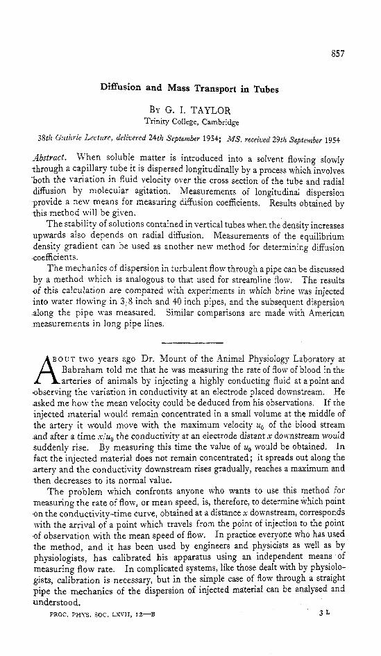
constancy of rate of flow. In later experiments constancy of flow was obtained b y fixing apparatus which removed fluid from the downstream end of the tube at a constant rate. One obvious way to do this is to fix to the downstream end of the experiment tube a capillary of much smaller bore. Another is to connect it with a cylinder whose volume is altered at a constant rate by a piston operated by a micrometer screw. Figure 5 shows the measured distribution of potassium

x (em) Figure 5. Distribution of c for KMnO, after 11 minutes In tube 0.0504 cm diameter.

permanganate in a tube 0.0504cm diameter after the flow had been going for 11 minutes. Initially the colourwas concentrated in the first few centimetresof the tube. It will be seen that the distribution is very close to the error curve which is marked. The dispersion is therefore as predicted and, comparing the parameter of the error curve in figure 5 with the formula (2), it was found that K = 0.0459 cm2 sec- l . Since U = g = 0.167 cm sec-l, the diffusion coefficient D, found from (l), is

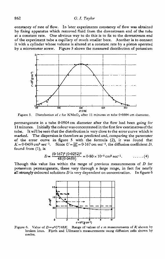
Though this value lies within the range of previous measurements of D for potassium permanganate, these vary through a large range, in fact for nearly all strongly coloured solutions D is very dependent on concentration. In figure 6

Figure 6 . Value of broken lines. circles.

c x l O ' ( g cm-J) D=a2U2/48K. Range of values of c in measurements

Fiirth and Ullmann's measurements using diffusion of K shown cells shown

38th Guthrie Lecture 863

-:.he range of concentrations covered by each experiment and the value obtained by applying equations (2) or (3) together with (1) are shown. The experimental results of Furth and Ullman (1927), who used diffusion cells, are also shown.

It is clear from the comparison shown in figure 6 that the measurement of dispersion might provide a much simpler technique for measuring c than the use of diffusion cells with all their attendant practical difficulties, but when D is not independent of c the formulae (2) and (3) are not accurate. In such cases the only practical methods for measuring c are, either to measure diffusion between pairs of solutions of slightly different concentrations, a method which cannot be used when concentrations are estimated colorimetrically, or to use only the type of experiment envisaged in (3), i.e. to introduce the solution at one end of the tube, which is initially filled with pure solvent, and maintain a constant flow of the solution.

The reason why this type of experiment can be analysed, and experiments in which the diffusion of an initially concentrated mass is measured cannot be interpreted, was originally pointed out by Boltzmann. He showed that when diffusion depends on concentration there is one case in which successive distribu- tions of concentration are all similar to one another, namely that in which the solution and solvent are each initially uniform and are separated by a plane surface. Boltzmann showed that at time t after diffusion started the concentration is a function of 5 = x t-1’2 only, and that

. . . . . (5)

Thus D can be determined €or the whole range of concentrations which occur in the experiments if c can be measured accurately as a function of 5 .

I tried applying this formula to my measurements of dispersion to obtain K instead of D as a function of 5, but when I calculated D from the values of K so obtained I found considerable differences between my values and those given in Landolt and BBrnstein’s tables. Such is my respect for these famous tables that I thought I must be wrong, but on looking up the original authors quoted I found that without exception all the measurements of diffusion of dyes and strongly coloured substances-covering many pages of the tables-are based on the equation (3), which is only correct when D is independent of e.? To get a n idea of how big the error might be I calculated the distribution of concentration for an ideal case in which D varies as e-Bc. I found that when ,!I is chosen so that this ideal variation is near the variation given in Landolt and Bornstein over the range used in the experiment, the error which the authors quoted in those tables could have made was in some cases greater than 50%.

It seems, therefore, that it is worth while to develop the dispersion apparatus so that it can make measurements of concentration accurately enough for use in deducing K from Boltzmann’s integral and then finding D from (1). I am now -engaged on this work.

DISPERSION IN TURBULENT FLOW The success of the method I have described in predicting the dispersion of

a dissolved salt along a pipe through which a non-turbulent stream is flowing -encouraged me to try whether the same physical principles could not be applied t o turbulent flow. The part played by radial diffusion in the former case must

t This criticism does not apply to all the diffusion measurements reported in Landolt and BBrnstein’s tables. In other cases Boltzmann’s method was used.

864 G. I . Taylor

be replaced by turbulent radial transport in the latter. Few measurements of radial transport of matter in pipe flow seem to exist, but every measurement 0:' pipe friction is automatically a measurement of radial transport of momentum, and there are vast numbers of these. Though it is not possible to prove an exac: connection between the transport of matter and the transport of momentum in turbulent flow, Osborne Reynolds pointed out the consequences which would arise if they were exactly analogous. Reynolds' analogy states that the virtual coefficient of diffusion for momentum is identical with that for heat or for any other transferable property of the fluid. In the case of radial transfer in a pipe this is expressed by the equation

..... . (6 )

where E is called the coefficient of turbulent transport, T is the turbulent stress a t radius Y , U is the velocity and nz the rate of transfer of matter in a radial direction. If T~ is the surface friction on the pipe the equation connecting T and

Since T~ is measured in pipe friction experiments, equations ( 6 ) and (7 ) provide a connection between m and ac/ar in terms of quantities previously measured. Though Reynolds' analogy is not demonstrably true, and in fact is demonstrably untrue in the case of free turbulence, it is found to be very nearly true in the case of turbulence near solid boundaries and in pipes, so that there is some justification for assuming it to be true in the present case.

The equation of continuity, that is the equation which expresses the fact that none of the dispersing material is lost during the process of dispersion, can be used in a way which is analogous to its use in the case of molecular diffusion. Considering as before only cases where the dispersing material is spread over- a length which is great compared with the diameter of the pipe, it is found as before that, relative to axes which move with the mean speed of flow, material is dispersed along the pipe as though by a virtual coefficient of diffusion

Here e, is the ' friction velocity ', which is defined by'the equation

A more familiar method for expressing the results of pipe friction experiments is

where y is a non-dimensional friction coefficient, U the mean speed of flow and p the density of the fluid.

so that (8) can be expressed in the form

is 7 = ToY/a. ......( 7 )

K= lO.lav,. ...... (8)

T0=/3V'a2. ..... . (9)

7 0 = Y(4P UZ> ...... (10)

v d U = V Y Y P ) , ..... . ( 1 1 )

K = l O . l a U ( v , / U ) = 7 ~ 1 4 a U ~ y . . . . . . . (12)

Comparing (9) with (10)

This result (Taylor 1954 b) looks very simple, but the ideas behind it and the mechanism it envisages are not so simple. However, the problem of the dispersion of material injected into pipes is one of practical importance, and several ex- perimental investigations have been made which can be compared with the theoretical formula. The earliest was that of Allen and Taylor (1923), who wanted to measure the speed of flow in large pipes conveying water to pouer plants. They injected salt into a stream flowing through a straight 40-inch pipe

38th Guthrie Lecture

:,55 feet long and measured the conductivity at the far end. Their object was rot to measure the dispersion but to find out what point on the conductivity-time curve corresponds with the time taken by points travelling with the mean speed t 3 cover 355 feet. They measured the mean flow also by other methods and f m n d that the required point on the conductivity-time curve was that at which the concentration was a maximum, as the present theory predicts. They did r.ot discuss the dispersion, but their published conductivity-time curves look Lke error curves. This is in accordance with the theory which predicts that the ciistribution of concentration about a point which moves with the mean speed is

where s1 is the distance from the centre of the concentration. By fitting the best error curve to one of Allen and Taylor’s observed distributions a value K = 2.18 x lo3 cm2 sec-l was found. In this experiment U = 105 cm sec-’ and U = 20 x 2.540 = 50.8 cm, so that, taking theviscosityofwateras 0.01 1, the Reynolds number of the flow was R = 105 x SO.SjO.Oll= 9.7 x lo5. At this Reynolds number the resistance coefficient is such that Ulvz=26. T o compare theory with observation it is convenient to calculate the measured value of (K/aU)( U/v,), which according to (12) should be 10.1. In the experiment just described this is

c = (const)t-1’2 exp ( - x,2/4Kt) . . . . . . (13)

. . . . (14)

‘The agreement between this and the theoretical value 10 1 is better than one would be justified in expecting from the nature of the experiment, and in fact another of Allen and Taylor’s experiments yielded K/cI‘L‘.= 11.7 when subjected to the same analysis.

In .Wen and Taylor’s experiments the measurements from which dispersion can be derived were only incidental to their main purpose. More recently dispersion in pipes has become important because very long pipes are used to convey fluids to great distances. Different grades of oil, say gasoline and Diesel oil, are transported successively in the same pipe. The pipe is not emptied between successive periods of use, so that there is a zone of mixture in which the surface of separation between two miscible fluids is dispersed along the pipe. It is of economic importance to know how much of each fluid is contaminated by mixture with the other. Hull and Kent (1952) have investigated this question by injecting a radioactive substance into a 10-inch pipe 152 miles long and measuring its dispersion at various points along its course when U = 81 7 cm sec-l. Figure 7 shows the concentration-time curves at stations 13.8, 43.1 and 108.5 miles from the point of injection. Error curves have been superimposed on the observed points, and these have been shifted so that their axes lie on the centre line of the figure. It will be seen that the dispersion is very closely gaussian, but when K is deduced from them it is found that K/az. , is larger than 10.1. It varies from 12.4 for the station nearest to the point of injection to 22.5 at 182 miles. The theoretical formula applies to a straight pipe, so that it is hardly to be expected that it would apply accurately to a pipe which accommodates itself to the hills and valleys over which it passes, but the discrepancy is more than I should have expected in view of the good agreement which was found in other large-scale experiments.

Smith and Schulze (1948) describe measurements with pipes 440 miles long in which two products A and B followed one another. At various points along

The ordinates therefore represent t--x U.

866 G. I . Taylor

the pipe samples were drawn off, and from these the length, S, of pipe in which the mixture changes from 1% A and 992, B to 99% A and 1% B as found. Using the theoretical formula ( 3 ) with (12) to calculate S I found that

where x is the length of the pipe between the entry and the point of measurement The comparison displayed in table 1 between the values of S measured in a 12-inch pipe and those calculated using (15) shows very good agreement.

S2 = 437ax(v,/ U ) . . . ...( 15)

t -x /U (sec)

Figure 7. Dispersion in a 10-inch pipe (Hull and Kent 1952).

When I made the theoretical analysis I did not know of the existence of these large-scale experiments, so, with the help of Dr. T. H. Ellison, I set up apparatus in the Cavendish Laboratory to measure dispersion in a pipe 0.9 cm diameter Table 1. Comparison between Calculated Values of S and those observed by

Smith and Schulze (1948) in a Long Pipe Line

x (feet)

322186 661109

1018301 1402896 1526085 2033803 2279538

1 0 - 4 ~

5.9 5.76 5.84 5.91 5.79 5.79 4.50

Utv, 25.4 25 4 25 4 25 4 25.4 25 4 24 6

S (feet) equation (15)

1670 2390 2970 3480 3870 4190 4340

(feet) x (miles) observed 1770 61 2425 12.T 2890 193 3505 265 3895 327 4360 385 4670 132

and 16 metres long. Salt was injected by a spring gun at one point and the conductivity at a point 16 metres downstream was recorded on a rotating drum camera. The conductivity-time curve so found was nearly gaussian in the middle but was not quite symmetrical particularly when the Reynolds number

3 8 t h Gu th rie Lecture 807

of the flow was low. This, I think, was due to the fact that in that case an appreciable amount of the brine was in the laminar boundary layer close to the wall where the Reynolds analogy does not hold.

It will be seen that at Reynolds number 1.2 x lo4, where the conductivity-time curve deviates consider- ably from the gaussian form, K/ao, is 12.8, which is well above the theoretical value., bu t at R = 1.9 x IO4 K / m , is 10.0, which is very close to the calculated value.

T h e results of these experiments are given in table 2.

Note. The values of U/vL for the curved pipe and for the rough pipe were nicasured. T h e values for the straight smooth pipe were taken from a curve representing previous experimental results at the appropriate value of R.

3 8 t h Gu th rie Lectu re 807

of the flow was low. This, I think, was due to the fact that in that case an appreciable amount of the brine was in the laminar boundary layer close to the wall where the Reynolds analogy does not hold.

It will be seen that at Reynolds number 1.2 x lo4, where the conductivity-time curve deviates consider- ably from the gaussian form, K/ao, is 12.8, which is well above the theoretical value., bu t at R = 1.9 x IO4 K / m , is 10.0, which is very close to the calculated value.

T h e results of these experiments are given in table 2.

'rable 2 Pipe Ucmjsec R Ulv, Kl(w,

40-inch (Allen and Taylor) 105 9.7 \ 10' 26.0 10.0

!:inch smooth x=1631 cm 222 1.9>(10' 17.5 104

$-inch rough x=245 cm 146 1.3 X 1 0 4 6.73 1 0 . 5 :-inch curved x=250 cm 113 0 . 9 ~ 1 0 ~ 15.0 21.9

9 inch smooth x=322 cm 222 1 . 9 ~ 1 0 4 17.5 11.6

:-inch smooth x=1631 cm 136 I .2x104 16.1 f2.X

{-inch curved x=250 cm 202 1 . 7 ~ 1 0 ~ 16.1 15.0

Note. The values of U/vL for the curved pipe and for the rough pipe were nicasured. T h e values for the straight smooth pipe were taken from a curve representing previous experimental results at the appropriate value of R.

Pipe 40-inch (Allen and Taylor)

9 inch smooth x=322 cm !:inch smooth x=1631 cm :-inch smooth x=1631 cm $-inch rough x=245 cm :-inch curved x=250 cm {-inch curved x=250 cm

'rable 2 U cmjsec

105 222 222 136 146 113 202

R Ulv, Kl(w, 9.7 \ 10' 26.0 10.0

1.9>(10' 17.5 104 1 . 2 ~ 1 0 4 16.1 f2.X 1.3 X 1 0 4 6.73 1 0 . 5 0 . 9 ~ lo4 15.0 21.9 1 . 7 ~ 1 0 ~ 16.1 15.0

1 . 9 ~ 1 0 4 17.5 11.6

Figure 9. Dispersion in a very rough #-inch pipe. Figure 9. Dispersion in a very rough #-inch pipe.

868 G. I. Taylor

The theory should apply to a rough pipe though not to a curved pipe. A pipe 24 metres long was artificially roughened by first wetting the inner wall with an adhesive and then pouring sand down it. Figures 8 and 9 show the record obtained and figure 9 the corresponding conductivity-time curve. Though the resistance coefficient was increased 6; times, the value of K/av,, namely 10.5, was still close to the theoretical value 10.1. When the 0.9 cm pipe was bent into a circle about 3 feet diameter, Klav , was increased about 50% at R= 1.7 x lo4. These results are also given in table 2.

EFFECTS OF GRAVITY (a) Tube horizontal.

In the preceding pages it has been tacitly assumed that the effect of gravity on the dispersion is negligible. To estimate the error involved in this erroneous assumption I calculated the dispersive power of gravity when the small variation of density due to dissolved material of concentration c can be represented by the expression

p=po(l t-ac). Here p and p o are the densities of the solution and the pure solvent, o! has a value which can easily be measured and is found in most cases to be of order 1. When the tube is horizontal the effect of gravity is to give rise to a current from high density to low along the lower half of the tube and a counter current along the top. This produces a dispersion which turns out to be negligible compared with that due to convection under the conditions of my experiments.

. . . . . . (16)

(b) Tube vertical.

If there is no mean flow the solute will merely be transported upwards by molecular diffusion when the solution is below a lighter solvent, but when the heavier solution is above the solvent the equilibrium might be expected to be unstable. The heavier solution would fall down into the solvent producing a downward current and the solvent so displaced would form a rising counter current. The solute in the downward current would then diffuse into the rising current of solvent and so lose the excess of density over that of the fluid at the same level which drives the current. The analysis of this process leads to the condition that equilibrium becomes stable and vertical currents stop when the vertical gradient of concentration, dcldz, becomes less than 67.94Dp/gpaa4. Here D is the coefficient of diffusion, 2a the diameter of the tube, g the acceleration of gravity and p the viscosity. In an experiment where a solution is in contact with a lighter solvent contained in a vertical tube below it, dc/dz is initially very large, so that vertical currents will be set up. Gradually, however, the critical value will be approached and the currents will stop. The only means of vertical transport is then molecular diffusion which is very slow. If, therefore, the vertical gradient of concentration is measured after the currents have stopped, a measure of Dp/gpaa4 is obtained. Since p, g , p , a and a can be measured, the experiment provides a method for measuring D. If variations of D, /I and 0:

with c are disregarded a very simple method for measuring D is to observe how

The case when the tube is vertical is much more interesting.

3Sth Guthrie Lecture S 69

far down the tube the solute penetrates. If this is represented by 2, the value Qf D isgpaa4co/67.94pZ. Using this method I have obtained values of D which lie within the ranges of previous measurements.

REFERENCES ALLEN, C. XI., and TAYLOR, E. A., 1923, Trans. Amer. Soc. Mech. Eizgrs, 45, 285. FORTH, R., and ULLMAN, E., 1926, Kolloidzschr., 41, 307. .GRIFFITHS, A., 191 1, Proc. Plzys. Soc., 23, 190. HULL, D. E., and KENT, J. IV., 1952, Industr. Engng Chem., 44, 2745. SMITH, S. S., and SCHULZE, R. K., 1948, Petrol. Evgr, 19,94 ; 20, 330. TAYLOR, Sir GEOFFREY, 1953, Proc. Roy. Soc. A, 219, 186; 1954 a, Ibid., 225,173; 1951 b,

Ibid., 223, 446.