A 21-point finite difference scheme for 2D frequency-domainelastic wave modelling

Bingluo Gu1,2 Guanghe Liang1,3 Zhiyuan Li1,2

1Key Laboratory of Mineral Resources, Institute of Geology and Geophysics, The Chinese Academy of Sciences,Beijing 100029, China.

2College of Earth Sciences, University of The Chinese Academy of Sciences, Beijing 100049, China.3Corresponding author. Email: lgh@mail.iggcas.ac.cn

Abstract. The 21-point finite difference scheme for the frequency-space domain elastic wave forward modelling isdesigned through optimising the impedance matrix, especially calculating the spatial derivative terms and the massacceleration terms of the elastic wave displacement equation as accurately as possible. Comparative tests show that the21-point finite difference scheme is much better in grid dispersion, memory requirement, and computation time than the 9-point scheme and slightly better than the 25-point scheme. The 21-point finite difference scheme is ~15% lower in memoryconsumption and computing time than the 25-point scheme. The numerical examples show that the 21-point finite differencescheme is valid in the sense of the numerical simulation of ideal models.

Key words: 21-point finite difference scheme, computing time, dispersion, frequency domain, memory consumption.

Received 22 October 2012, accepted 7 April 2013, published online 8 May 2013

Introduction

Since frequency domain forward modelling was proposed byLysmer and Drake (1972), there have been many improvedvarietal frequency domain modelling methods developed(Pratt, 1990; Jo et al., 1996; Štekl and Pratt, 1998; Shin andSohn, 1998;Min et al., 2000), including frequency-space domainforward modelling (Marfurt, 1984; Marfurt and Shin, 1989).Compared with conventional time domain forward modelling,frequency-space domain forward modelling has two advantages(Min et al., 2000; Liao et al., 2009a, 2009b). First, it uses animplicit finite difference (FD) operator and so has no timeaccumulated error. Second, it is suitable for parallelcomputation and can flexibly select frequency bands formodelling, because each single frequency component it uses isindependent. There are also, however, two problems with thismodelling method: severe grid dispersion and huge memoryconsumption, which have restricted its application to a largeextent. To date, the frequency-space domain FD forwardmodelling of seismic waves has been used mainly in twomodelling directions: acoustic wave forward modelling andelastic wave forward modelling. In these two directions,improving the design of the FD scheme is one of the mainways of increasing modelling efficiency. With respect to theacoustic wave modelling, the following schemes have beenproposed: one 5-point FD scheme proposed by Pratt (1990); atime saving staggered grid FD scheme by Luo and Schuster(1990); an optimised 9-point FD scheme proposed by Jo et al.(1996); and a 25-point FD scheme byShin and Sohn (1998).Withrespect to the elasticwavemodelling, the following schemes havebeen proposed: a 9-point FD scheme proposed by Pratt andWorthington (1990); another 9-point FD scheme proposedthen by Štekl and Pratt (1998) through coordinate rotation; anda 25-point finite difference scheme by Min et al. (2000) throughweighted average. Compared with Pratt’s scheme, Štekl andPratt’s (1998) scheme can reduce the number of grid point to 9

per shear wavelength, and the errors are held within 1%. Minet al.’s (2000) 25-point FD scheme achieved considerablesuccess, requiring only 2.7 grid points per shear wavelength toachieve an upper limit of error of 1% in phase velocity. However,a lot of modelling practices and studies (Saenger et al., 2000;Hustedt et al., 2004; Operto et al., 2009; Ren et al., 2009; Liaoet al. 2009a, 2009b, 2011; Yin et al., 2006; Li et al., 2011) showthat it is still possible for both the memory requirement and thecomputing time to be reduced through further improvement of theFD scheme.

As an effort towards improvement, we propose a 21-point FDscheme for the 2D elastic wavemodelling in the frequency-spacedomain. In this paper, we give thought to design, compare it withthe 9-point scheme and the 25-point scheme, and check itsvalidity.

A 21-point finite difference scheme

The memory consumption and the computing time in thefrequency-space domain forward modelling are dependent onthe bandwidth, the position of every non-zero stripe relative to themain diagonal and the singularity of the impedance matrix. Weassume each diagonal of the impedancematrix is a stripe.We callit a non-zero stripe if the diagonal contains a non-zero element.Therefore, the problems of huge memory consumption and slowcomputing speed could be solved by reasonably optimising theimpedance matrix.

The grid of the 21-point FD scheme designed throughoptimising the impedance matrix is shown in Figure 1a.Obviously, the number of the grids in the horizontal directionis more than that in the vertical direction. That is because bynumbering the grids vertically first and thenmoving horizontally,the grid set shown in Figure 1a yields a narrow-bandwidthimpedance matrix. If the grids are numbered horizontally firstand thenvertically, the bandwidth of the impedancematrixwill be

CSIRO PUBLISHING

Exploration Geophysics, 2013, 44, 156–166http://dx.doi.org/10.1071/EG12064

Journal compilation � ASEG 2013 www.publish.csiro.au/journals/eg

wide. For comparison, the grids of a 9-point scheme and a 25-point scheme are shown in Figure 1b and Figure 1c, respectively.

Optimisation of the impedance matrix can be achievedthrough calculating the spatial derivative terms and the mass

acceleration terms of the elastic wave displacement equation asaccurately as possible. The elastic wave displacement equation inthe homogeneous 2D frequency-space domain can be expressedas:

(a)

(b)

(c)

Fig. 1. Grids of three FD schemes: (a) 21-point scheme, (b) 9-point scheme and (c) 25-point scheme.

Table 1. Initial and optimal values of weighting coefficients.

Coefficients Initial Optimal

a1 0.5 0.35914a2 0.3 0.11290a3 0.1 –0.02656a4 0.1 0.01948a5 0.05 –0.00032a6 0.05 0.01214a7 0.01 –0.00303b1 0.6 0.76111b2 0.3 0.38310b3 0.5 0.47481b4 0.3 0.14459b5 0.1 0.01437b6 0.05 –0.00915c 0.8 0.46567d 0.3 –0.02441e 0.1 0.07496f 0.9 0.78123

Table 2. Characteristics of the impedancematrix for three FD schemes(nx is the number of grid points in the horizontal direction).

9-point FDscheme

25-point FDscheme

21-point FDscheme

Bandwidth 2(2nx+3) 2(4nx+5) 2(2nx+7)Number of diagonal 3 5 3Number ofnon-zero stripe

17 41 29

Distribution ofnon-zero stripe

7–3–7 9–9–5–9–9 11–7–11

Table 3. Number of points per shear wavelength for three FD schemesto achieve an upper limit of error of 1% in phase velocity.

9-point FDscheme

25-point FDscheme

21-point FDscheme

G 9 2.7 3.3

21-point finite difference scheme Exploration Geophysics 157

ðlþ 2mÞ q2U

qx2þ m

q2Uqz2

þ ðlþ mÞ q2V

qxqzþ ro2U ¼ �FðoÞ

ðlþ 2mÞ q2V

qz2þ m

q2Vqx2

þ ðlþ mÞ q2U

qxqzþ ro2V ¼ �GðoÞ

8>><

>>:

ð1Þ

where U and V are the spectra of horizontal and verticaldisplacement components, respectively; F and G are the bodyforce terms; l and m are the Lamé constants; o is the angularfrequency; and r is the density of the medium.

In order to calculate the spatial derivative terms and the massacceleration terms as accurately as possible, we construct theirFD operators.

Thus, for the horizontal displacement spectrum U in thespatial derivative terms, we have the following FD operators:

q2Uqz2

� b1Dx2

½cðUiþ1;j � 2Ui;j þ Ui�1;jÞ þ d

4ðUiþ2;j � 2Ui;j

þ Ui�2;jÞ þ e

9ðUiþ3;j � 2Ui;j þ Ui�3;jÞ�

þ b2Dx2

½cðUiþ1;j�1 � 2Ui;j�1 þ Ui�1;j�1Þ þ d

4ðUiþ2;j�1

� 2Ui;j�1 þ Ui�2;j�1Þ þ e

9ðUiþ3;j�1 � 2Ui;j�1

þ Ui�3;j�1Þ�

þ b2Dx2

½cðUiþ1;jþ1 � 2Ui;jþ1 þ Ui�1;jþ1Þ þ d

4ðUiþ2;jþ1

� 2Ui;jþ1 þ Ui�2;jþ1Þ þ e

9ðUiþ3;jþ1 � 2Ui;jþ1

þ Ui�3;jþ1Þ� ð2Þ

q2Uqz2

� b3Dz2

ðUi;jþ1 � 2Ui;j þ Ui;j�1Þ

þ b4Dz2

ðUi�1;jþ1 � 2Ui�1;j þ Ui�1;j�1Þ

þ b4Dz2

ðUiþ1;jþ1 � 2Uiþ1;j þ Uiþ1;j�1Þ

þ b5Dz2

ðUi�2;jþ1 � 2Ui�2;j þ Ui�2;j�1Þ

þ b5Dz2

ðUiþ2;jþ1 � 2Uiþ2;j þ Uiþ2;j�1Þ

þ b6Dz2

ðUi�3;jþ1 � 2Ui�3;j þ Ui�3;j�1Þ

þ b6Dz2

ðUiþ3;jþ1 � 2Uiþ3;j þ Uiþ3;j�1Þ

ð3Þ

q2Uqxqz

� f

4DxDz

ðUiþ1;jþ1 � Uiþ1;j�1 � Ui�1;jþ1 þ Ui�1;j�1Þð4Þ

where Dx and Dz are the grid intervals of horizontal andvertical directions, respectively, and bi (i = 1, 2, 3, . . ., 6), c, d,e and f are optimalweighting coefficients for the spatial derivativeterms.

For the mass acceleration terms, we have the following FDoperator:

ro2U � ro2½a1Ui;j þ a2ðUiþ1;j þ Ui�1;j þ Ui;j�1 þ Ui;jþ1Þþ a3ðUiþ1;jþ1 þ Uiþ1;jþ1 þ Ui;j�1 þ Ui�1;j�1Þþ a4ðUiþ2;j þ Ui�2;jÞ þ a5ðUiþ3;jÞ þ ðUi�3;jÞþ a6ðUiþ2;j�1 þ Ui�2;j�1 þ Uiþ2;jþ1 þ Ui�2;jþ1Þþ a7ðUiþ3;j�1 þ Ui�3;j�1 þ Uiþ3;jþ1 þ Ui�3;jþ1Þ�

ð5Þwhere aj (j= 1, 2, 3, . . ., 7) are optimal weighting coefficientsfor the acceleration terms.

0

20

(a)

(b)

(c)

40

60

80

0

20

40

60

N =

98

N = 98

80

0

0

20

20 40 60 80

40

60

80

Fig. 2. Structure of the impedance matrix for three FD schemes: (a) 9-pointscheme, (b) 25-point scheme and (c) 21-point scheme.

158 Exploration Geophysics B. Gu et al.

For the vertical displacement spectrum V in the spatialderivative and mass acceleration terms, we have similar FDoperators.

The optimal weighting coefficients aj, bi, c, d, e and fmentioned above can minimise the grid dispersion andnumerical anisotropy. The weighting coefficients should be

independent of Poisson’s ratio, and using the Gauss-Newtonmethod given by Min et al. (2000), we determine their optimalvalues, as listed in Table 1.

In addition, our sampling of propagation angle, Poisson’sratio, and the number of points in theminimumwavelength showsthat these optimal weighting coefficients are independent of the

1.25P-wave dispersion curve

S-wave dispersion curve

Poisson’s ratio = 0.25

1.20

9–0°

9–15°

9–45°

21–0°

21–15°

21–30°

21–45°

25–0°

25–15°

25–45°

25–30°

9–30°

1.15

1.10

1.05

0.95

0.90

0.85

Vph

/V0

0.80

0.75

1.00

1.25

1.20

1.15

1.10

1.05

0.95

0.90

0.85

0.80

0.750 0.05 0.10 0.15 0.20 0.25

1/G0.30 0.35 0.40 0.45 0.50

1.00

(a)

(b)

Fig. 3. Dispersion curves obtained by plotting the normalised phase velocity of three FD schemes for different propagationangles of 0�, 15�, 30� and 45�: (a) compressional wave with a Poisson ratio of 0.25; (b) shear wave with a Poisson ratio of 0.25;(c) compressionalwavewith aPoisson ratio of 0.4; and (d) shearwavewith aPoisson ratio of 0.4.The green curves are for the9-pointscheme; the red curves are for the 21-point scheme; and the blue curves for the 25-point scheme.

Table 4. Memory requirements tested for three FD schemes and six models. Note: D is the grid interval, D= dx= dz.

Model type 9-point FD scheme 25-point FD scheme 21-point FD schemeMemory (GB) Grid size (m) Memory (GB) Grid size (m) Memory (GB) Grid size (m)

Homogeneous >10 D= 2.2 1.6116 D= 7.3 1.4877 D= 6.0Horizontal layer >10 D= 2.2 1.6530 D= 7.3 1.3654 D= 6.0Dipping layer >10 D= 2.2 1.6724 D= 7.3 1.3683 D= 6.0Curved surface >10 D= 2.2 1.6521 D= 7.3 1.3567 D= 6.0Step >10 D= 2.2 1.6749 D= 7.3 1.3845 D= 6.0Salt dome >10 D= 2.2 1.6732 D= 7.3 1.3924 D= 6.0

21-point finite difference scheme Exploration Geophysics 159

internal structureof themodel.Thismeans that theyare applicableto any models, including inhomogeneous models.

In designing the 21-point FD scheme, we also introduce thePML absorbing boundary condition as its boundary condition(Berenger, 1994).

Therefore, the 21-point FD scheme makes the impedancematrix show a structure different from those of the 9-point FDscheme and the 25-point FD scheme (Figure 2) and somecharacteristics of these FD schemes are shown in Table 2.

Comparison of three finite difference schemes

Dispersion

In order to compare the grid dispersions of the 21-point FDscheme, the 9-point FD scheme, and the 25-point FD scheme, weplotted the phase velocities at different propagation angles(0�, 15�, 30� and 45�) to the number of grid point under

1.25

1.20

1.15

1.10

1.05

0.95

0.90

0.85

Vph

/V0

0.80

0.75

1.00

1.25

1.20

1.15

1.10

1.05

0.95

0.90

0.85

0.80

0.75

1.00

P-wave dispersion curve

S-wave dispersion curve

0 0.05 0.10 0.15 0.20 0.25

1/GPoisson’s ratio = 0.4

0.30 0.35 0.40 0.45 0.50

9–0°

9–15°

9–45°

21–0°

21–15°

21–30°

21–45°

25–0°

25–15°

25–45°

25–30°

9–30°

(c)

(d )

Fig. 3. (Continued)

0

10

50 100 150 200 250 350 400 450 500300

20

Tim

e (s

)

Frequency (Hz)

30

40

50

60

21–point9–point25–point

70

Fig. 4. Computing time-frequency curves of individual singlefrequency wave fields recorded by the elapsed-time indicator for threeFD schemes.

160 Exploration Geophysics B. Gu et al.

Vp = 2000 m/sVrs = 1300 m/s

= 2073 kg/m3

(a)

(b) (c)

(d) (e)

Homogeneous space model

Source

0.250

0.25

0.50

0.75

1.00

Dep

th (

km)

Distance (km)

0

0.25

0.50

0.75

1.00

0.50 0.75 1.00 0.25 0.50 0.75 1.00

Fig. 5. Homogeneous space model: (a) velocity structure; (b) snapshot of horizontal displacementcomponent at 250ms by the frequency-space domain forward modelling; (c) snapshot of horizontaldisplacement component at 250ms by the conventional second-order FD time domain forwardmodelling;(d) snapshot of vertical displacement component at 250ms by the frequency-space domain forwardmodelling, (e) snapshot of vertical displacement component at 250ms by the conventional second-orderFD time domain forward modelling.

Table 5. Computing time tested for three FD schemes and six models.

Model type 9-point FD scheme 25-point FD scheme 21-point FD schemeTime (103 s) Grid (m) Time (103 s) Grid (m) Time (103 s) Grid (m)

Homogeneous 31.5687 D= 2.2 4.3764 D= 7.3 3.6499 D= 6.0Horizontal layer 27.6983 D= 2.2 4.4023 D= 7.3 3.7192 D= 6.0Dipping layer 20.0081 D= 2.2 4.4032 D= 7.3 3.7214 D= 6.0Curved surface 21.6982 D= 2.2 4.4053 D= 7.3 3.7235 D= 6.0Step 21.9687 D= 2.2 4.4134 D= 7.3 3.7534 D= 6.0Salt dome 22.6589 D= 2.2 4.4075 D= 7.3 3.7433 D= 6.0

21-point finite difference scheme Exploration Geophysics 161

Poisson’s ratios 0.25 and 0.4 (Figure 3). The results show that thedispersion of the 9-point scheme is very large, while thedispersions of the 21-point scheme and the 25-point schemeare similar, both being relatively small. Moreover, in order tokeep the error of phase velocities within 1%, the 9-point schemerequires 9 points per shear wavelength, the 25-point schemerequires only 2.7 points, and the 21-point scheme needs 3.3points (Table 3). It follows that the 21-point scheme is betterin dispersion than the 9-point scheme, but not less than the25-point scheme.

Memory requirement

In order to compare the memory consumption of the abovethree FD schemes, we tested them with six different specificmodels: homogeneous space model, horizontal layer model,dipping layer model, curved interface model, step model, andsalt dome model. The size of each of the six models is 840m� 840m. In testing, we used the same LU sparse matrixfactorisation solver. The test standards and conditions also areconsistent: the time sampling interval is 1mswith a time samplinglength of 1 s; the seismic source is a Ricker wavelet with adominant frequency of 25Hz; the loading is a concentratedforce on the vertical displacement component, i.e. at thecoordinate point of x = 420m and z = 20m of the model; andthe boundary applied is the PML absorbing boundary. In order toachieve better absorption and reduce the computationalrequirement, we set the thickness of one side of the PMLlayers around the model to be 30 dx or 30 dz (Qian et al.,2013). We also applied the PML boundary condition to thesurface boundary.

Our testswere carried out keeping the sameaccuracy for all theFD schemes. The test results are summarised in Table 4. It can beseen from Table 4 that the memory occupied for the 9-pointscheme is the highest, that for the 25-point scheme is much lowerthan that for the 9-point scheme, and that for the 21-point schemeis the lowest, although only slightly lower than that for the 25-point scheme (~15%).

Computing time

In order to compare the computing time of these three FDschemes, we used the same models, test standards and testconditions as those in the above section. Our tests were alsocarried out keeping the same accuracy for all the FDschemes. Thetest results that we obtained by adding up the costs for allfrequencies are summarised in Table 5. It can be seen fromTable 5 that the computing time for the 9-point scheme is thelongest, that for the 25-point scheme is much shorter than that forthe 9-point scheme, and that for the 21-point scheme is theshortest, although only slightly shorter than that for the 25-point scheme (~15%).

As we know, one advantage of the frequency domain forwardmodelling is that every single frequency wave field can becalculated independently for serial computation, and thus thecomputing time of the total frequency wave field can bedetermined directly by adding computing time of individualsingle frequency wave fields. It can also be seen from Figure 4that for the 21-point FD scheme, the computing time of a singlefrequency is the shortest and is stable over the entire frequencyrange; for the 25-point FD scheme, the computing time of a singlefrequency is longer in a few frequency wave fields; and for the 9-point FD scheme, the computing time of a single frequencyincreases sharply with frequencies in the high frequency range.

Numerical examples

We checked the validity of the 21-point FD scheme on threemodels through numerical simulation. The method of numericalsimulation carried out on the three models is the frequency-spacedomain forward modelling except that, for comparison, theconventional second-order FD time domain forward modellingwas also carried out, especially on the first model.

The first model is a homogeneous space model, whose size is1000m � 1000m and whose velocity structure is shown inFigure 5a. The simulation conditions used are as follows: thegrid intervals are dx= dz = 5m; the seismic source is a Rickerwavelet with a dominant frequency of 25Hz; the loading is a

1.0Receiver #1

(a) (b)

(c) (d)

Receiver #2

Receiver #3 Receiver #3

0.5

0.0

–0.521–point25–point

21–point25–point

21–point25–point

21–point25–point

–1.0

1.0

0.5

0.0

–0.5

–1.00.20 0.25 0.30 0.35 0.40

Time (s)0.45 0.50 0.55 0.60 0.20 0.25 0.30 0.35 0.40 0.45 0.50 0.55 0.60

Fig. 6. Numerical solutions by the 25-point FD scheme (blue solid line) and numerical solutions by the 21-point FD scheme(red point symbol) for horizontal displacements at (a) receiver 1, (b) receiver 2, (c) receiver 3, and (d) vertical displacement atreceiver 3 of Figure 5a.

162 Exploration Geophysics B. Gu et al.

concentrated force on the vertical displacement component, thatis, at the coordinate point of x = 500mand z = 500mof themodel;the time sampling interval is 1ms with a time sampling length of1 s; and the boundary applied is the PML absorbing boundary. Inorder to achieve better absorption and reduce the computationalrequirement, we set the thickness of one side of the PML layers

around the model to be 30 dx or 30 dz (Qian et al., 2013).We alsoapplied the PML boundary condition to the surface boundary.

Figure 5b, c shows the snapshots of horizontal displacementcomponents at 250ms obtained by the frequency-space domainforward modelling and the conventional second-order FD timedomain forward modelling, respectively, while Figure 5d, e

0.0

Distance (km)

(a)

(b) (c)

(d ) (e)

Distance (km)

Dep

th (

km)

Dep

th (

km)

Tim

e (s

)

0.3 0.6 0.9 1.2

0.3 0.6 0.9 1.2

0.3 0.6 0.9 1.2 0.3 0.6 0.9 1.2

0.3 0.6 0.9 1.2

0.2

Source

3400

3200

3000

2800

2600

2400

2200

2000

0.4

0.6

0.8

1.0

1.2

0.0

0.2

0.4

0.6

0.8

1.0

1.2

0.0

0.2

0.4

0.6

0.8

1.0

1.2

Fig. 7. Two layer model: (a) velocity structure; (b) snapshot of horizontal displacement component at 500msby the 21-point FD scheme; (c) snapshot of vertical displacement component at 500ms by the 21-point FDscheme; (d) synthetic seismogram of horizontal displacement component by the 21-point FD scheme; and(e) synthetic seismogram of vertical displacement component by the 21-point FD scheme.

21-point finite difference scheme Exploration Geophysics 163

shows the snapshots of vertical displacement components at250ms obtained by the frequency-space domain forwardmodelling and the conventional second-order time domainforward modelling, respectively. The identity of the respectivesnapshots of horizontal and vertical components goes withoutsaying. No recognisable difference can be seen.

We still use the first model (see Figure 5a) for our comparisonof the numerical solutions obtained by the 21-point FD schemeand the 25-point FD scheme (Min et al., 2003, 2004). Figure 6showshorizontal displacements at receivers 1, 2 and3andvertical

displacement at receiver 3. In Figure 6, we can easily see that thenumerical solutions given by the 21-point FD scheme agree wellwith the numerical solutions given by the 25-point FD scheme.

The second model is a two layer model, whose size is1200m� 1200m and whose velocity structure is shown inFigure 7a. The simulation parameters used are as follows: thegrid intervals are dx= dz = 6m; the seismic source is a Rickerwavelet with a dominant frequency of 25Hz; the loading is aconcentrated force on the vertical displacement component, thatis, at the coordinate point of x = 600m and z = 20m of the model;

0.00.2 0.4 0.6 0.8 1.0 1.2

0.2 0.4 0.6 0.8 1.0 1.2 0.2 0.4 0.6 0.8 1.0 1.2

0.2

0.4

4500

4000

3500

3000

2500

2000

1500

0.6

0.8

1.0

1.2

0.0

0.0100 200 300 100 200 300

0.5

1.0Tim

e (s

)D

epth

(km

)

Distance (km)

Distance (km)

Source

Dep

th (

km)

1.5

0.2

0.4

0.6

0.8

1.0

1.2

(a)

(b)

(d) (e)

(c)

Fig. 8. Sigsbee2B model: (a) velocity model; (b) snapshot of horizontal component at 500ms;(c) snapshot of vertical component at 500ms; (d) synthetic seismogram of horizontal component, and(e) synthetic seismogram of vertical component.

164 Exploration Geophysics B. Gu et al.

the time sampling interval is 1ms with a time sampling length of1.2 s; the receivers are set on the surface. The boundary applied isthe same as that of the previous model.

The simulation result is perfect, reflecting the feature of thetwo layer model. This can be seen from Figure 7b–e. Figure 7b, care the snapshots of the horizontal and the vertical displacementat 500ms, respectively, in which the reflected and transmittedwaves are very clear at the interface, and the converted wave isalso evident. Figure 7d, e are the synthetic seismograms of thehorizontal and the vertical displacement, respectively, in whichthe P- and S-waves are very clear.

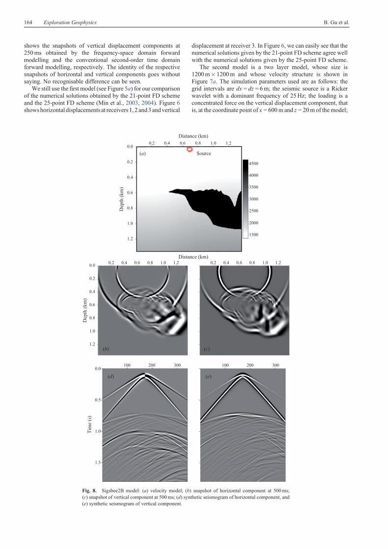
The third model is a Sigsbee2B model (Paffenholz et al.,2002). Strictly speaking, it is part of that model with a size of1360m� 1360m. The velocity structure is shown in Figure 8a.The simulation parameters are the same as those of the secondmodel, except that the grid intervals are dx= dz= 4m, the sourceis set at the coordinate point of x = 680m and z = 80m of themodel, and the time sampling length is 1.8 s. The other simulationparameters are the same as those of the second model.

Figure 8b–e shows a part of the simulation result. Figure 8b, cshows the snapshots of the horizontal and the verticaldisplacement at 500ms, respectively, from which it can beseen that the wave field is very complex and the events areclean and clear, and that the wave field energy in the high-speed body is weak, a feature for a high-speed body.Figure 8d, e shows the synthetic seismograms of the horizontaland the vertical displacement, respectively, in which reflectionsfrom the internal and the external of the high-speed body arevery clear and distinct, really reflecting the compositionaldifference between the internal and the external of the high-speed body.

The above modelling shows that the 21-point FD scheme isvalid in the sense of the numerical simulation of ideal models,although its validity in the sense of practical application requiresfurther work. However, the conventional second-order FD timedomain forward modelling on the first model verified the validityin some sense. Moreover, numerical anisotropy seems to be notreflected in the numerical simulation result as shown by thehomogeneous model in Figure 5, although the 21-pointscheme is an asymmetric scheme.

Conclusions

The 21-point FD scheme for the frequency-space domainelastic wave forward modelling is designed through optimisingthe impedance matrix, especially calculating the spatialderivative terms and the mass acceleration terms of the elasticwave displacement equation as accurately as possible.Comparative tests show that if you maintain the griddispersion at the same level, the 21-FD scheme is better inmemory requirement and computation time. On the contrary, ifyou maintain the memory requirement and computation time atthe same level, the 21-FD scheme is better in grid dispersion. Inotherwords, the 21-point FD schemeuses ~15% lessmemory andalso 15% less computing time than the 25-point scheme. Thenumerical examples show that the 21-point FD scheme is valid inthe sense of the numerical simulation of ideal models. Itsasymmetry does not produce any recognisable anisotropy inthe numerical simulation results.

Acknowledgements

We thank Shaozong Zhang for valuable comments and helpful suggestionsthat greatly improved the readability of this paper, andYoushanLiu for usefuldiscussions about the paper. Our sincere thanks also go to the reviewer Dr

Dong-JooMin and four anonymous reviewers for their constructive criticismsof our paper.

References

Berenger, J., 1994, A perfectly matched layer for the absorption ofelectromagnetic waves: Journal of Computational Physics, 114,185–200. doi:10.1006/jcph.1994.1159

Hustedt, B., Operto, S., and Virieus, J., 2004, Mixed-grid and staggered-gridfinite-differencemethods for frequency-domain acousticwavemodelling:Geophysical Journal International, 157, 1269–1296. doi:10.1111/j.1365-246X.2004.02289.x

Jo, C., Shin, C., and Suh, J., 1996, An optimal 9-point finite-differencefrequency-space 2-D scalar wave extrapolator:Geophysics, 61, 529–537.doi:10.1190/1.1443979

Li, G., Feng, J., and Zhu, G., 2011, Quasi-P wave forward modelling inviscoelastic VTI media in frequency-space domain: Chinese Journal ofGeophysics, 54, 200–207. [in Chinese]

Liao, J. P., Wang, H. Z., and Ma, Z. T., 2009a, Compression storage forfrequency-space domain 2-D elastic wave forward modelling: CPS/SEGBeijing 2009 International Geophysical Conference & Exposition.

Liao, J. P., Wang, H. Z., and Ma, Z. T., 2009b, 2-D elastic wave modellingwith frequency-space 25-point finite-difference operators: AppliedGeophysics, 6, 259–266. doi:10.1007/s11770-009-0029-7

Liao, J. P., Liu, H. X.,Wang, H. Z., Yang, T. C.,Wang, Q. R., Liu, X. H., andMa, Z. T., 2011, Study on rapid highly accurate acoustic wave numericalsimulation in frequency space domain: Progress in Geophysics, 26,1359–1363. [in Chinese]

Luo, Y., and Schuster, G., 1990, Parsimonious staggered grid finitedifferencing of the wave equation: Geophysical Research Letters, 17,155–158. doi:10.1029/GL017i002p00155

Lysmer, J., andDrake,L.A., 1972,Afinite-elementmethod for seismology, inB. A. Bolt, ed., Methods in computational physics: Academic Press Inc.11, 181–216.

Marfurt, K., 1984, Accuracy of finite-difference and finite-elementmodellingof the scalar and elastic wave equations: Geophysics, 49, 533–549.doi:10.1190/1.1441689

Marfurt, K., and Shin, C., 1989, The future of iterative modelling ingeophysical exploration, in E. Eisner, ed., Handbook of geophysicalexploration: I - Seismic exploration, 21 - Supercomputers in seismicexploration: Pergamon Press, 203–228.

Min, D., Shin, C., Kwon, B., and Chung, S., 2000, Improved frequency-domain elastic wave modelling using weighted-averaging differenceoperators: Geophysics, 65, 884–895. doi:10.1190/1.1444785

Min, D., Shin, C., Pratt, R., and Yoo, H., 2003, Weighted-averaging finite-element method for 2D elastic wave equations in the frequency domain:Bulletin of the Seismological Society of America, 93, 904–921.doi:10.1785/0120020066

Min, D., Shin, C., and Yoo, H., 2004, Free-surface boundary condition infinite-difference elastic wave modelling: Bulletin of the SeismologicalSociety of America, 94, 237–250. doi:10.1785/0120020116

Operto,S.,Virieux, J.,Ribodetti,A., andAnderson, J., 2009,Finite-differencefrequency-domain modelling of viscoacoustic wave propagation in 2Dtilted transversely isotropic (TTI) media: Geophysics, 74, T75–T95.doi:10.1190/1.3157243

Paffenholz, J., Mclain, B., Zaske, J., and Keliher, P., 2002, Subsalt multipleattenuation and imaging: observations from the Sigsbee2B synthetic dataset: 72nd Annual International Meeting, SEG, Expanded Abstracts,2122–2125.

Pratt, R., 1990, Frequency-domain elastic wave modelling by finitedifferences: a tool for crosshole seismic imaging: Geophysics, 55,626–632. doi:10.1190/1.1442874

Pratt, R., and Worthington, M., 1990, Inverse theory applied to multi-sourcecross-hole tomography, Part 1: acoustic wave-equation method:Geophysical Prospecting, 38, 287–310. doi:10.1111/j.1365-2478.1990.tb01846.x

Qian, J., Wu, S. G., and Cui, R. F., 2013, Extension of split perfectlymatched absorbing layer for 2D wave propagation in poroustransversely isotropic media: Exploration Geophysics, 44, 25–30.doi:10.1071/EG12002

21-point finite difference scheme Exploration Geophysics 165

Ren, H., Wang, H., and Gong, T., 2009, Seismic modelling of scalar seismicwave propagation with finite-difference scheme in frequency-spacedomain: Geophysical Prospecting for Petroleum, 48, 20–26.

Saenger, E., Gold, N., and Shapiro, S., 2000, Modelling the propagation ofelastic waves using a modified finite-difference grid: Wave Motion, 31,77–92. doi:10.1016/S0165-2125(99)00023-2

Shin, C., and Sohn,H., 1998,A frequency-space 2-D scalarwave extrapolatorusing extended 25-point finite-difference operators: Geophysics, 63,289–296. doi:10.1190/1.1444323

Štekl, I., and Pratt, R., 1998, Accurate viscoelastic modelling by frequency-domain finite differences using rotated operators: Geophysics, 63,1779–1794. doi:10.1190/1.1444472

Yin, W., Yin, X. Y., and Wu, G. C., 2006, The method of finite difference ofhigh precision elastic wave equations in the frequency domain and wave-field simulation: Chinese Journal of Geophysics, 49, 561–568.[in Chinese]

166 Exploration Geophysics B. Gu et al.

www.publish.csiro.au/journals/eg